Easily Implemented Methods of Radiometric Corrections for Hyperspectral–UAV—Application to Guianese Equatorial Mudbanks Colonized by Pioneer Mangroves

Abstract

Hyper-DRELIO (Hyperspectral DRone for Environmental and LIttoral Observations) is a custom, mini-UAV (unmanned aerial vehicle) platform (<20 kg), equipped with a light push broom hyperspectral sensor combined with a navigation module measuring position and orientation. Because of the particularities of UAV surveys (low flight altitude, small spatial scale, and high resolution), dedicated pre-processing methods have to be developed when reconstructing hyperspectral imagery. This article presents light, easy-implementation, in situ methods, using only two Spectralon^® and a field spectrometer, allowing performance of an initial calibration of the sensor in order to correct “vignetting effects” and a field standardization to convert digital numbers (DN) collected by the hyperspectral camera to reflectance, taking into account the time-varying illumination conditions. Radiometric corrections are applied to a subset of a dataset collected above mudflats colonized by pioneer mangroves in French Guiana. The efficiency of the radiometric corrections is assessed by comparing spectra from Hyper-DRELIO imagery to in situ spectrometer measurements above the intertidal benthic biofilm and mangroves. The shapes of the spectra were consistent, and the spectral angle mapper (SAM) distance was 0.039 above the benthic biofilm and 0.159 above the mangroves. These preliminary results provide new perspectives for quantifying and mapping the benthic biofilm and mangroves at the scale of the Guianese intertidal mudbanks system, given their importance in the coastal food webs, biogeochemical cycles, and the sediment stabilization.

1. Introduction

Mangroves are highly productive ecosystems, which dominate the intertidal zone of tropical and subtropical coasts. Mangroves fulfil numerous ecological functions (habitats, breeding grounds, nursery, carbon sink, water filtration, sediment retention) [1]. Mangroves grow on fine sand to silty sediments in areas protected from high-energy wave action, mainly found in depositional coastal environments, such as the deltaic, lagoon, or mudflat systems. However, these ecosystems are more and more threatened by global changes, which include anthropogenic pressures (i.e., pollution, urbanization, fisheries, aquaculture…) as well as climate change (i.e., increase of temperatures and sea level, high-intensity cyclones…) [2,3]. This is even truer on the coasts of countries with rapidly increasing human demography. Management and restoration of these ecosystems has become highly necessary. An initial step toward adequate management is monitoring, which can be done using different techniques. Remote sensing appears to be a valuable approach for field observations given the practical difficulties to access and carry out in situ measurements in those complex and dynamical systems (for reviews, see, for example, [4,5,6]). Indeed, remote sensing offers synoptic information, allowing the detection, classification, or mapping of mangroves and the monitoring of their spatial organization and temporal evolution. In Amazon-influenced coastal areas, as in large tropical deltaic coasts, mangroves grow over vast intertidal mudflats. Thus, mangroves ecosystems cannot be characterized only through the spatial coverage of mangrove trees. Indeed, they also include a variety of geomorphological forms, such as the creeks, ridges, runnels, sediment platforms, and depressions—that can be observed from aerial view—and, depending on pixel resolution of the imaging sensors, the spatial coverage and density of the trees and the age of the forests. This spatial heterogeneity of habitats increases the complexity in signal processing of remote sensing data, concerning the identification and quantification of the trees and intertidal benthic constituents.

Over the last decades, remote sensing has undergone major developments resulting from a combination of technological progress in platforms, sensors, data processing, and data availability. Among all the possible remote sensing issues (e.g., meteorology, military applications, cartography, topography, oceanography, geology, natural hazards, etc.), several applications make use of the radiometric properties of the scene, such as computation of classification indices, spectral unmixing, or radiative transfer modelling [7]. Indeed, each substrate has a specific spectral signature (i.e., the reflectance as a function of wavelength), which can be used for material identification or classification. This requires a high spectral fidelity and the measurement of a wide spectrum at high resolution, which are only offered by hyperspectral sensors [8]. Until then, hyperspectral data were mainly collected from airborne or satellite platforms, as the Hyperion satellite imaging spectrometer, with a spatial resolution from about 50 cm for low altitude (<1500 m) airborne surveys [9] to dozens of meters for high altitude surveys [10]. VNIR (visible and near infrared) hyperspectral sensors provide hundreds of continuous spectral bands between 400 nm and 1100 nm. Such a spectral richness allows accurate mapping and classification of complex environments, such as vegetation and ground features. The development of airborne sensors and high spatial resolution hyperspectral images meets a large audience in environmental research and particularly in forestry. Numerous studies over a significant range of forest types, using various classification algorithms, have emerged during this decade [11,12,13,14]. That underlines the applicability and potential of hyperspectral images for mapping vegetation over various spatial footprints and spatial resolutions. Hyperspectral monitoring of mangrove forests has mostly been developed since the early 2000s from aircraft vessels along the southeastern coast of the USA [15], the Indian coast [16,17,18], the Australian coast [12], and the southeastern coast of Asia [19,20,21].

Considering their ability to provide quick and cost-effective observations with great flexibility in survey planning, the use of unmanned aerial vehicles (UAVs) or drones has boomed over the last decade. Because of limited payload, small UAVs are mostly equipped with RGB or VNIR multispectral cameras. Nevertheless, drone-based hyperspectral sensing solutions also arose in the last few years [22]. These hyperspectral–UAV systems can now complement airborne and satellite approaches for hyperspectral imaging and bridge the gap in resolution and spatial coverage between remote data and ground-based measurements. In flying at low altitude (below 150 m), UAVs offer the opportunity to collect very high spatial resolution data, capturing a larger number of details. Furthermore, hyperspectral–UAV systems also allow a great flexibility regarding devices configuration and flight plan adjustments or times at which surveys are carried out. Surveys of mangrove forests by drones equipped with a hyperspectral camera mark a recent turning point in terms of image resolution and survey repeatability. The studies involving hyperspectral–UAV surveys of mangrove forests mostly took place on the southeastern coast of China [19,23,24]. To our knowledge, there has been no previous study, involving a hyperspectral–UAV camera, conducted over mangrove forests in South America and French Guiana.

These drone platforms offer interesting capabilities, provided one has adequate algorithms for georeferencing and radiometric corrections. Several studies refer mainly to helicopters or fixed-wing UAVs, designed to support large and heavy (>5 kg) payloads [25,26,27,28]. However, helicopters generate high frequency vibrations and require specially trained operators. Fixed-wing platforms provide long and smooth flights but are wide UAVs, which require a large area, suitable for take-off and landing. On the contrary, multi-rotor UAVs have a shorter autonomy and generate high-frequency vibrations; however, being able to take-off and land vertically and fly at a steady altitude, they are more suited to field areas of few hectares [22]. Usually considered as “mini-UAVs” (<20 kg), they support lighter payloads (<5 kg) [29,30,31]. Stuart et al. [22] propose a review of relatively low-cost, field-deployable hyperspectral devices, particularly UAV-based devices, for environmental monitoring. These drone-based technologies include point-based spectrometers, push broom sensors, and, more recently, hyperspectral frame cameras. These systems differ in their spatial coverage, in the tradeoff between spatial and spectral resolutions, and in how easy image reconstruction and georeferencing are with their use. Dedicated pre-processing methods usually have to be developed for data georeferencing and radiometric corrections. Specific algorithms for radiometric corrections also need to be elaborated, given that classical models for geometric, atmospheric, and radiometric corrections are not suited to UAV data, considering the flight height and temporal and spatial scales of UAV surveys [8,29,32,33,34].

The electromagnetic radiation received by the sensor is referred to as the spectral radiance. In reality, the sensor records raw digital numbers (DN). In many studies, the parameter of interest is the ratio of upwelling radiation in a given direction toward the sensor (radiance) to downwelling radiation (irradiance), known as remote sensing reflectance. The latter is a key parameter, sometimes denoted as the spectral signature, which theoretically allows a description of the nature of the studied surface, independently of the sensor, viewing geometry, sun azimuth, elevation, or the weather conditions. Thus, radiometric corrections, consisting in converting the DN recorded by the sensor into ground reflectance values, can rely on different approaches, often requiring the acquisition of complementary field data. This process is necessary for data interpretation or diachronic comparisons. The geometric, radiometric, and spectral properties of the instruments can be partly characterized and calibrated through laboratory tests, but this requires having a dedicated test bed [34]. Regarding radiometric corrections, Saari et al. [32] proposed a drone equipped with downwelling and upwelling irradiance sensors to record illumination conditions during the flight. However, adding embedded sensors increases the payload, which is generally the main limit of UAV systems [29,34]. Another approach consists of using additional systems on the ground, especially white reference panels, to convert the sensor’s digital number (DN) to reflectance [8,33,34,35].

Drone monitoring has proven particularly useful as a non-destructive data acquisition technic in dynamic and complex coastal and estuarine systems where ground-based field surveys are very difficult, especially for monitoring purposes in unconsolidated temperate mudflats [36] and along the French Guiana (FG) littoral zone, for sandy beaches and mangrove-colonized mudbanks [37,38]. Belonging to the largest mudflat in the world, the French Guianese coastline, dominated by mangroves, is indeed experiencing extremely rapid morphological changes in response to the large amounts of Amazonian sedimentary inputs [39]. Mangrove ecosystems development or disappearance accompanies the alternation of Amazonian mudbanks accretion and erosion phases along the north coast of South America between the Amazon and Orinoco Rivers [40,41]. At a regional scale, geomorphology changes rapidly and becomes favorable to the development of different mangrove stand ages [40,41] and specific benthic biodiversity, which in turn modify the geomorphological evolution of the mudbanks. Indeed, as the mud consolidates, the substrate elevation increases and the flooding time during each tidal cycle decreases. As results of such dynamics, biological processes within sediments are intense, enhanced by both benthic biofilm development and bioturbation by crabs [37,42]. In these geographical areas, the benthic biofilm is as important as the mangrove trees in terms of carbon biomass and as a source of organic matter for the coastal food webs and regional biogeochemical cycles [43,44,45,46].

In this natural and complex context, it is necessary to explore the spatial and spectral richness of hyperspectral–UAV data. A reliable analysis of these data requires a first step of radiometric pre-processing. The present study describes and implements a radiometric correction method on UAV in situ data, collected along a gradient of pioneer mangroves in French Guiana, using the Hyper-DRELIO drone. Radiometric corrections here encompass calibration and in situ standardization. The method we propose is easy to implement, without adding embedded sensors and with limited additional equipment.

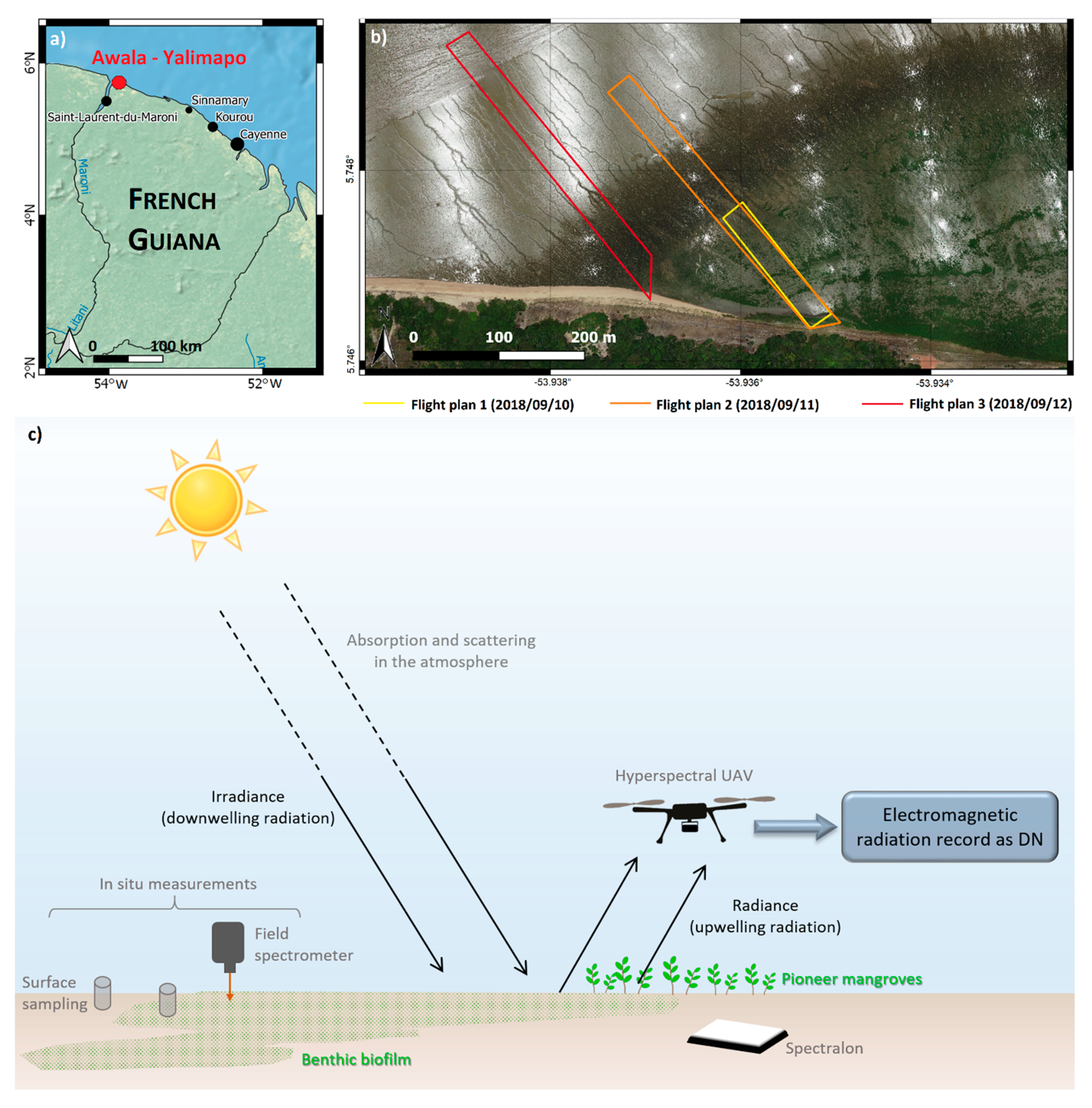
2. Study Area and Survey Setup

The field campaign took place in the northwestern part of French Guiana (Awala-Yalimapo; Figure 1a,b), during the dry season in September 2018. Besides the natural dynamics of mudbanks, this region is submitted to additional anthropogenic pressure following polder erosion, making the area unstable [47]. Preliminary results showed that mangroves colonized the consolidated part of the mudbank in 2015 and the oldest trees were about 3 years old at the time of our field measurements campaign. The northwestern part of the mudbank was characterized by unconsolidated bare mud.

Tides at this location are semidiurnal in the study area with high spring tide ranges up to 3.5 m and a mean tidal range of 1.68 m (https://maree.shom.fr for “Les Hattes” site—access on 1 April 2020).

Taking advantage of the flexibility of drone-based systems, we tailored the survey to examine benthic biofilm development in relation to the tidal cycle, carrying out the flights at low tide during spring tide. As depicted in Figure 1c, hyperspectral drone surveys were synchronized with in situ measurements for radiometric correction and validation purposes.

3. Materials and Methods

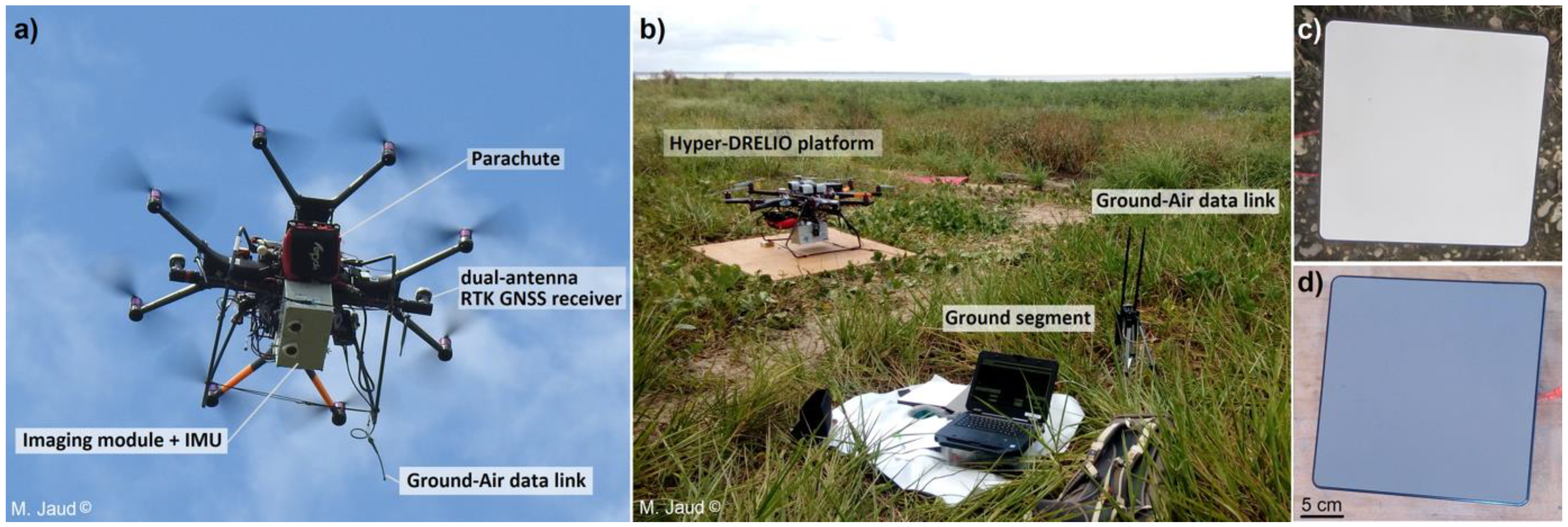
3.1. Hyperspectral UAV

The integration of the light push broom hyperspectral sensor onboard the multirotor UAV, called Hyper-DRELIO (Hyperspectral DRone for Environmental and LIttoral Observations), is described in Jaud et al. (2018). The system is composed of an electric octocopter platform (Figure 2a,b), an imaging module, and a navigation module, synchronized via CPU (central processing unit) timestamps. To complement this system, a ground segment allows sensor parametrization, data quality control during the flight, and flight parameter control.

The drone has a diameter of 1.2 m, weighs 13.4 kg, and can handle a payload of 5 kg (including batteries, cables, navigation modules, and imagery modules). Considering the duration of ascent and descent phases and a safety cushion, the programmed flight plan duration must not exceed 7–8 min [30]. The onboard flight control system of the drone is composed of a global navigation satellite system (GNSS) and an autopilot, run by DJI^® iOSD^® software. The navigation module, which measures position and orientation during the flight, is composed of a dual-antenna RTK (real time kinematics) GNSS receiver with a baseline of 85 cm and an Ekinox-D^® (SBG System^®) inertial motion unit (IMU). The hyperspectral camera, a Micro-Hyperspec^® VNIR (Headwall^®), is a push broom (or line-scanning) system, collecting reflected light through an image slit. The principle of operation of this camera relies on holographic diffraction, using gratings and mirrors to split monochromatic light into 250 spectral bands, ranging between 400 nm and 1000 nm, with 1.85 nm of spectral resolution. The manufacturer carried out a wavelength calibration beforehand, in order to determine the correspondence relationship between imaging spectrometer probe elements and the central wavelength. On the CCD sensor matrix, rows collect spatial, across-track information and columns record the spectral content of the signal. Values for each element of the matrix are expressed as 12-bit DN (i.e., values between 0 and 4096). The camera is equipped with a fixed focus lens, focused to infinity. Aperture and sensor gain G were adjusted before the flight, depending on the illumination conditions, in order to avoid saturation of the CCD cells. The integration time remained fixed during the flight, which required that there is no major variation of the illumination conditions during the flight (around 12 min duration).

The acquisition frame rate was parametrized to 50 Hz, which is compatible with a UAV speed of around 3–4 m/s (close to the lower boundary for drone stability). At 50 m above ground level, the configuration chosen for this study, the swath was 45 m wide and the across-track ground resolution was 4.5 cm. With a speed of 3 m/s, the along-track ground sampling was about 6 cm.

A line-by-line geo-registration procedure was proposed in [30] for geometrical pre-processing of hyperspectral data. The accuracy of this direct georeferencing method is on the order of 1 m for a flight at 50 m of altitude. The quality of the georeferencing process is limited by several factors: mechanical stability of the platform, the timing accuracy, and more particularly, the resolution and accuracy of the proprioceptive sensors (GNSS receivers and IMU). This geo-registration to realign and geo-reference the push broom data is non-intrusive and preserves fragile substrates, such as mud. Ground control points would have allowed a more accurate estimation of the geo-registration error, but their installation would have been very destructive to the substrate.

With such characteristics, the Hyper-DRELIO system is adequate to cover areas of approximately 10,000 m² and to study objects ranging from 10 centimeters to several meters. The main advantage of the drone is that it can perform repeated overflights over an area that changes over time (such as the mudflat during a tidal cycle). However, push broom technology is not suitable for imaging moving objects, such as waves or animals. In addition, the drone platform is dependent on weather conditions and flights cannot be performed in rain or strong winds. Cloudy skies are the preferred conditions to avoid sun glint effects; however, all flights during the mission took place in sunny conditions.

3.2. Ground-Based Measurements

Ground positioning measurements were performed using RTK-differential GNSS, achieving centimetric accuracy after post-processing of the base station. The device used for this study was a Topcon^® HiPer V GNSS receiver. The same base receiver was used both for ground measurements and for the navigation module of Hyper-DRELIO.

The in situ data for radiometric standardization and validation were measured with a GER 1500 field spectrometer (developed by Spectra Vista Corporation^®), providing fast, at-target radiance measurements from 350 nm to 1050 nm. Each measurement was triplicated and averaged. A white Spectralon^TM panel with a reflectivity of 99% allowed an indirect measurement of the irradiance. This Spectralon (Figure 2c) was a 40 × 40 cm white reference panel made of a fluoropolymer, which is highly reflective (the highest diffuse reflectance of any known material) and has Lambertian behavior [48]. This Spectralon^TM panel is placed on flat ground near the take-off area. For the initial calibration, a grey Spectralon^TM (Figure 2d), with a reflectivity of 20%, was also used. As 20% reflectivity is closed to the reflectance of bare mud, this grey Spectralon^TM was also used to adjust the parametrization of the hyperspectral camera (aperture and sensor gain G) before the flight.

The spectrometer measurements were carried out in a flight-synchronous manner on different types of substrates. In order to limit the movements of the operators, which were very slow, difficult, and very destructive for the mudflat, these measurements were carried out around a fixed platform placed on the mud.

3.3. Radiometric Correction Method

Radiometric corrections aim to convert the raw digital numbers (DN) recorded by the sensor into remote sensing reflectance. Once the reflectance is computed, hyperspectral images can be exploited in different ways, such as computation of spectral indices for classification (e.g., [49,50]), study of the red edge position (e.g., [51]), or spectral unmixing [52].

For hyperspectral measurements acquired with drones, radiometric corrections were realized using complementary in situ data. Given the practical challenges in carrying out surveys in mangrove or mudflat areas, the proposed method must be easy to implement, without adding embedded sensors and with as little equipment as possible. Computational routines to apply corrections were implemented in Matlab^®, including several steps, which are summarized in Figure 3. During the acquisition, the signal was impacted by noise, called the dark current (DC) [53], which is partly function of sensor temperature and partly integration time. In our case, this DC is assumed steady. Furthermore, as the survey was focused on mudflats, the topographic effects could be neglected. Finally, as the flight altitude remained low (<150 m), we hypothesized that the at-target radiance was equal to the at-sensor radiance at 50 m height [54]. To validate this hypothesis, raw spectra (in DN) were measured by the hyperspectral camera above the white Spectralon^TM panel, both from the ground and in flight. The mean difference between the “on ground” spectra and “on flight” spectra was about 7.5% with a standard deviation of 5.3% and a preserved shape of spectra.

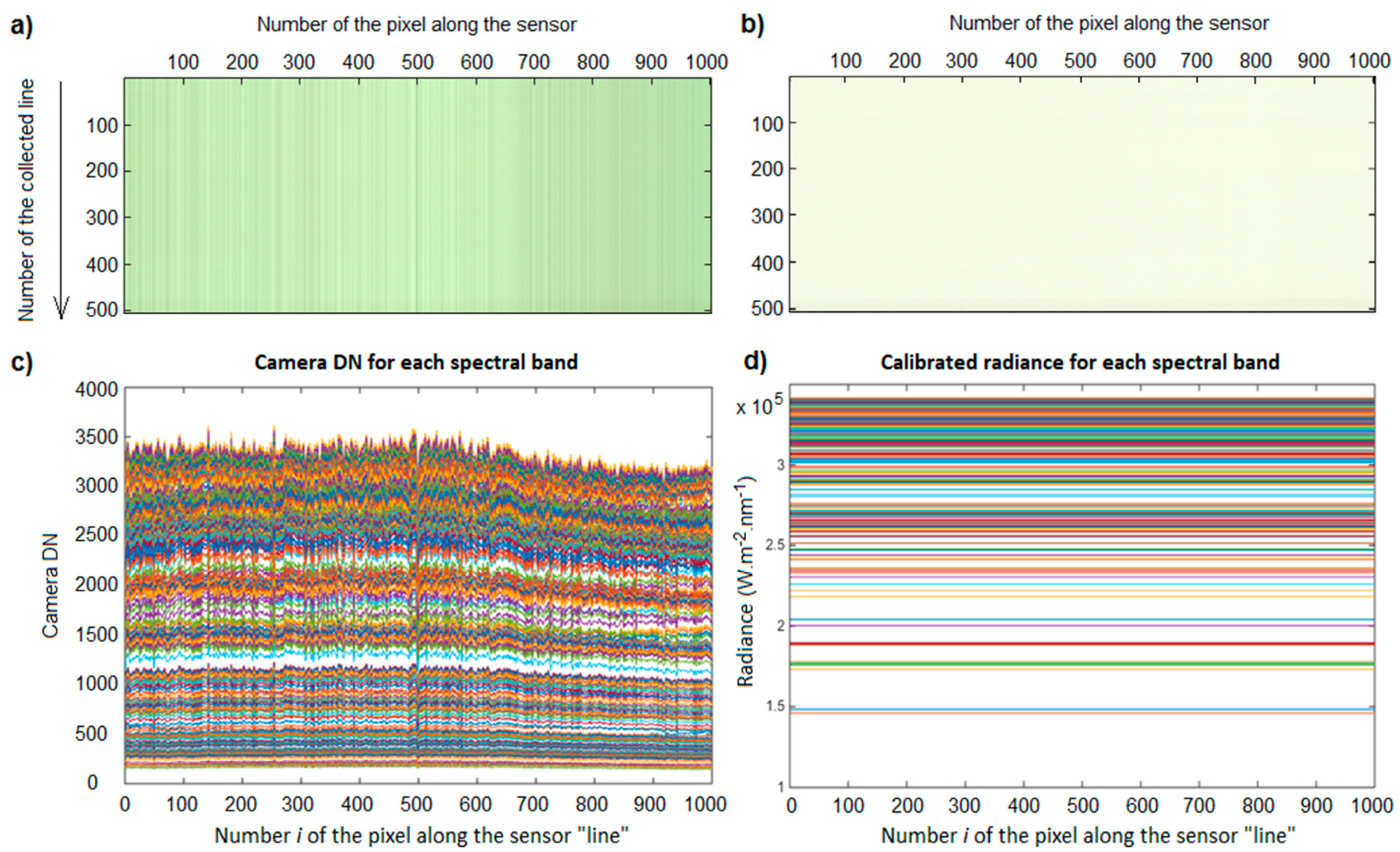
3.3.1. Initial Calibration

Hyperspectral images suffer from variations or distortions of the spectrogram along the CCD array (possibly caused by the quality of the dispersive element or misalignments of the light from the slit). This results in vertical “stripes” in our push broom images. This spatial dependence of DN, and particularly its decrease towards the image edges, is called the “vignetting effect” for frame sensors [53] and corresponds rather to the “lining effect” for push broom sensors.

The calibration parameters aim to compensate for this effect and to convert DN to physical units of radiance. We chose an image-based calibration method, and we assumed a linear relationship between the DN and the at-sensor radiance [54,55], according to the following empirical transfer function (Equation (1)):

Rad_C(λ, i) = a(λ, i) × DN_C(λ, i)/G_C + b(λ, i)

(1)

With the following:

• λ: wavelength (nm);
• i: index of the pixel in the sensor array;
• Rad_C: at-sensor radiance (W·m⁻²·sr⁻¹) during calibration step;
• G_C: sensor gain during calibration step;
• DN_C: digital number collected during calibration step;
• a, b: calibration coefficients.

To calculate a and b coefficients, we considered the radiance measured by the field spectrometer above both white and grey Spectralon panels, and the DN measured simultaneously by the hyperspectral camera. Each Spectralon was thus targeted simultaneously by the GER1500 field spectrometer and by the hyperspectral camera, while the drone was on the ground, in such a way that the field spectrometer and the hyperspectral camera were at the same distance from the Spectralon panel and the measurements were synchronized. The a and b coefficients were calculated per pixel and per spectral band, according to the following equations (Equation (2)):

$$\{\begin{array}{l}a\left(\mathsf{\lambda },\mathrm{i}\right)=G_C\times \frac{Ra{d}_{Sp1}\left(\mathsf{\lambda },\mathrm{i}\right)-Ra{d}_{Sp2}\left(\mathsf{\lambda },\mathrm{i}\right)}{\left[D{N}_{Sp1}\left(\mathsf{\lambda },\mathrm{i}\right)-D{N}_{Sp2}\left(\mathsf{\lambda },\mathrm{i}\right)\right]}\\ b\left(\mathsf{\lambda },\mathrm{i}\right)=Ra{d}_{Sp1}\left(\mathsf{\lambda },\mathrm{i}\right)-\frac{a}{G_C}D{N}_{Sp1}\left(\mathsf{\lambda },\mathrm{i}\right)\end{array}$$

(2)

With the following:

• Sp1, Sp2: ID of each Spectralon used for the calibration;
• Rad_{Sp1, Sp2}: radiance (W·m⁻²·sr⁻¹) measured by the field spectrometer above the Sp1 (respectively, Sp2) Spectralon;
• DN_{Sp1, Sp2}: digital number collected by the hyperspectral camera above the Sp1 (respectively, Sp2) Spectralon.

To avoid local effects due to possible wear marks on the Spectralon surface, several hyperspectral lines were recorded by the hyperspectral camera (500 lines were selected and averaged) and 8 spectra were measured by the field spectrometer from various directions and averaged. To visually confirm the efficiency of this calibration, a and b coefficients were applied to DN_Sp1 (respectively, DN_Sp2), measured above the white Spectralon (respectively, the grey Spectralon). The results above the white Spectralon, before and after calibration, are depicted in Figure 4, representing, in natural colors, the hyperspectral lines collected by the camera.

This calibration step was carried out once (at least for the entire field campaign) and the coefficients were then applied to all the different following surveys. The a and b coefficients are exported to a “calibration file”, which will be reused in the in situ standardization step.

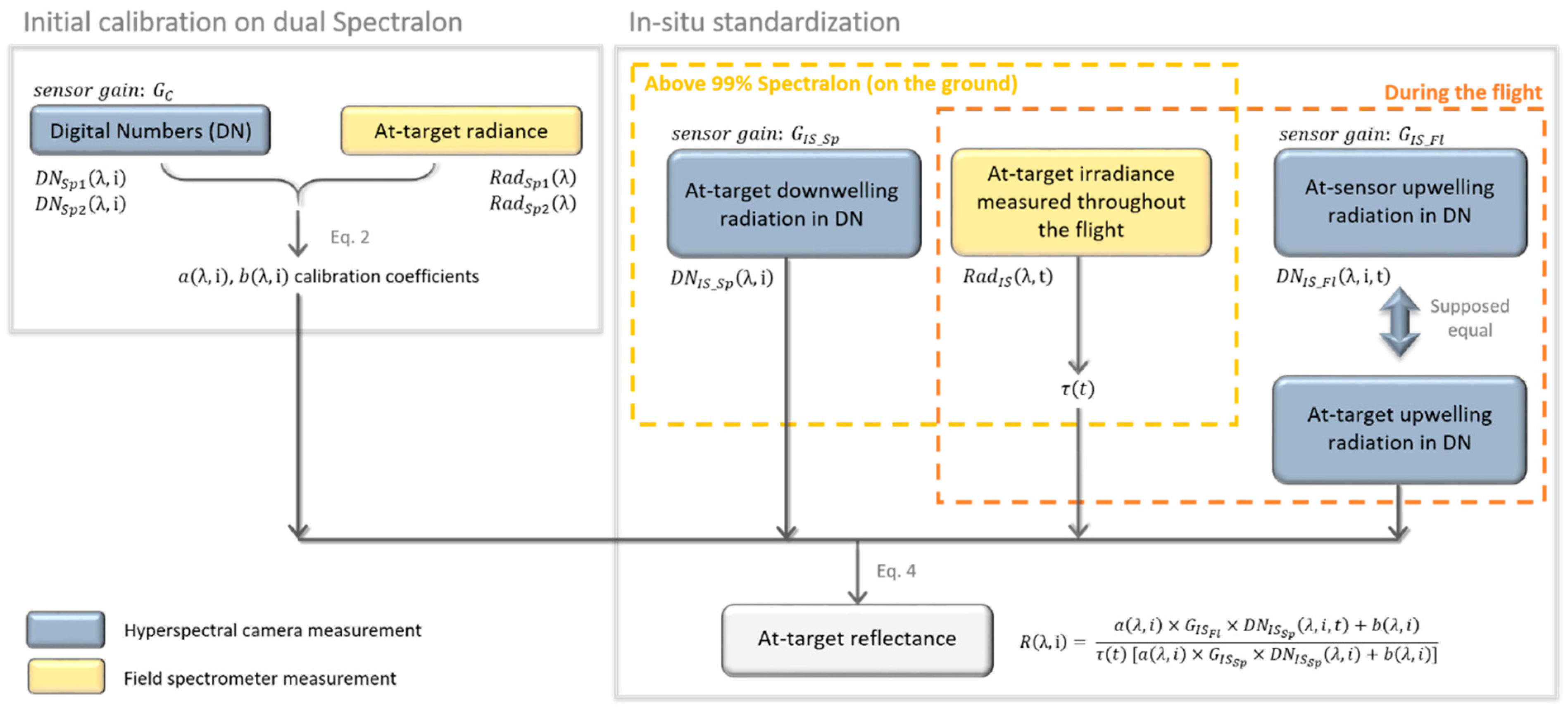
3.3.2. In Situ Standardization

For each in situ survey, the collected data DN_IS are calibrated using the a and b coefficients (Equation (1)). Applying Equation (1) enables compensation for the lining effects and provides a result with physical units of radiance; however, this is not the real in situ at-target radiance. Indeed, considering Equation (2), the a and b coefficients are related to the illumination conditions at the moment of the dual Spectralon measurements with both hyperspectral sensors during the calibration step. Therefore, Equation (1) needs to be standardized to the in situ atmospheric conditions at the time of the survey.

For each survey, before the flight, the irradiance was indirectly measured on the white 99% Spectralon panel, by the hyperspectral camera, held about 30 cm above the Spectralon. During this step, the operators had to be careful not to create shade on the Spectralon, which can be complicated when placing the drone-borne camera above it. As for the calibration step, to avoid local effects due to possible wear marks on the Spectralon surface, several hyperspectral lines recorded by the camera were selected and averaged. The irradiance before the flight was also measured with the field spectrometer, which was targeted to the white 99% Spectralon almost simultaneously with the hyperspectral camera, and from the same distance of about 30 cm, to serve as a reference for temporal variations of irradiance.

The sensor gain (G_IS) at the time of the survey also needed to be taken into account. The in situ sensor gain (G_IS) is adjusted before the flight, according to the illumination conditions, to avoid signal saturation. Therefore, it can be different from the gain G_C used during the calibration step. Besides, if the flown-over area is expected to have a low reflectivity, the in situ gain in flight (G_{IS_Fl}) can also be parametrized differently from the in situ gain used, above the 99% Spectralon G_{IS_Sp}.

The in situ reflectance was calculated by forming the ratio of the upwelling radiation to the downwelling radiation. This is given by Equation (3):

$$R\left(\mathsf{\lambda },\mathrm{i}\right)=\frac{a\left(\mathsf{\lambda },\mathrm{i}\right)\times \frac{D{N}_{I{S}_{Fl}}\left(\mathsf{\lambda },\mathrm{i},\mathrm{t}\right)}{G_{I{S}_{Fl}}}+b\left(\mathsf{\lambda },\mathrm{i}\right)}{a\left(\mathsf{\lambda },\mathrm{i}\right)\times \frac{D{N}_{I{S}_{Sp}}\left(\mathsf{\lambda },\mathrm{i}\right)}{G_{I{S}_{Sp}}}+b\left(\mathsf{\lambda },\mathrm{i}\right)}$$

(3)

With the following:

• G_{IS Sp}: sensor gain used during in situ measurements of the 99% Spectralon;
• G_{IS Fl}: sensor gain used during the in situ flight;
• DN_{IS Sp}: digital number collected in situ by the hyperspectral camera of the 99% Spectralon;
• DN_{IS Fl}: digital number collected in situ by the hyperspectral camera during the flight;
• R: resulting remote-sensing reflectance.

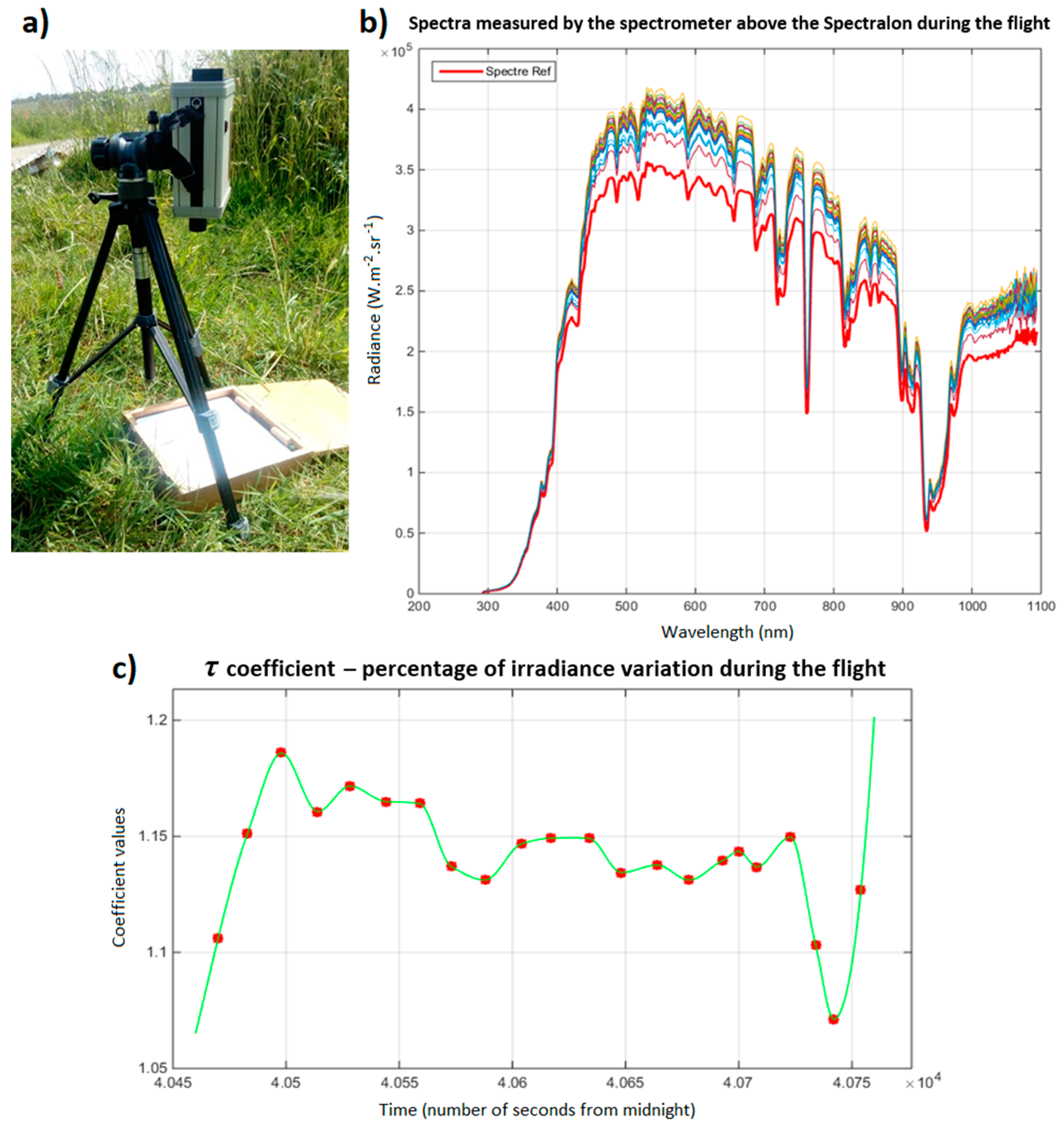
3.3.3. Taking Temporal Variations of Irradiance into Account

The illumination changes during data acquisition are generally pointed as a source of difficulties in hyperspectral surveys [22,56]. Our approach to addressing this issue is almost comparable to the “dual-spectrometer” method, proposed for a ground-based system in Bachmann et al. [48], and consists of monitoring illumination change using a reference panel, simultaneously with data acquisition [22].

To mitigate the variations of ambient light, the field spectrometer regularly recorded the irradiance above the white Spectralon (with a time-step from 10 s to 20 s) (Figure 5a). The internal clock of the field spectrometer was synchronized with the GPS time (used in the header file of the hyperspectral camera). We hypothesized that the shape of the irradiance spectra would vary linearly over time, mainly according to a single, time-dependent multiplying coefficient called τ (Figure 5b). The τ coefficients, calculated for each field spectrometer record, were then interpolated over time to obtain a coefficient for irradiance evolution (τ(t)) throughout the survey (Figure 5c). This dimensionless coefficient represents the percentage of irradiance variation in comparison to the irradiance measured just when the in situ standardization was performed (t0). Therefore, τ is equal to 1 when the illumination does not change, greater than 1 if the illumination increases, and lower than 1 if it decreases. To take into account the variations of irradiance, Equation (3) is changed into Equation (4):

$$R\left(\mathsf{\lambda },\mathrm{i}\right)=\frac{a\left(\mathsf{\lambda },\mathrm{i}\right)\times \frac{D{N}_{I{S}_{Fl}}\left(\mathsf{\lambda },\mathrm{i},\mathrm{t}\right)}{G_{I{S}_{Fl}}}+b\left(\mathsf{\lambda },\mathrm{i}\right)}{\mathsf{\tau }\left(\mathrm{t}\right)\times a\left(\mathsf{\lambda },\mathrm{i}\right)\times \frac{D{N}_{I{S}_{Sp}}\left(\mathsf{\lambda },\mathrm{i}\right)}{G_{I{S}_{Sp}}}+b\left(\mathsf{\lambda },\mathrm{i}\right)}$$

(4)

where the τ coefficient represents the percentage of irradiance variation during the flight.

To complete this procedure of radiometric corrections, a signal enhancement was performed, using a minimum noise fraction (MNF) transform, as implemented in ENVI^® software (modified from [57]). A forward transform is performed to manually identify the bands containing the coherent images and those containing noise-dominated images. Noise is removed from the data by performing an inverse transform using a spectral subset which only includes the bands with a high signal-to-noise ratio.

4. Results

With the configuration used, a flight of about 10 minutes can collect usable hyperspectral images (i.e., excluding take-off, landing, and turning phases) over an area of about 2.6 × 104 m² (2.6 ha), with a resolution of 4.5 cm × 6 cm. The reflectance spectra obtained at each pixel are inherent signatures of the targeted surfaces, resulting from the presence, the shape, and the position/orientation of specific absorption features, such as pigments, which compose the surface. For identification and classification purposes, the spectrum of each class of targets has to be uniquely characterized by its general shape, combined with local absorption or reflectance peaks.

The quality of the results is assessed in two ways:

(i) Firstly, by comparing the spectra obtained from Hyper-DRELIO imagery with spectra, measured by the field spectrometer on the same types of substrates or sediment coverage.

(ii) Secondly, by comparing spectra from Hyper-DRELIO imagery acquired at two different times on a surface assumed to be stable over time—in this case, sand.

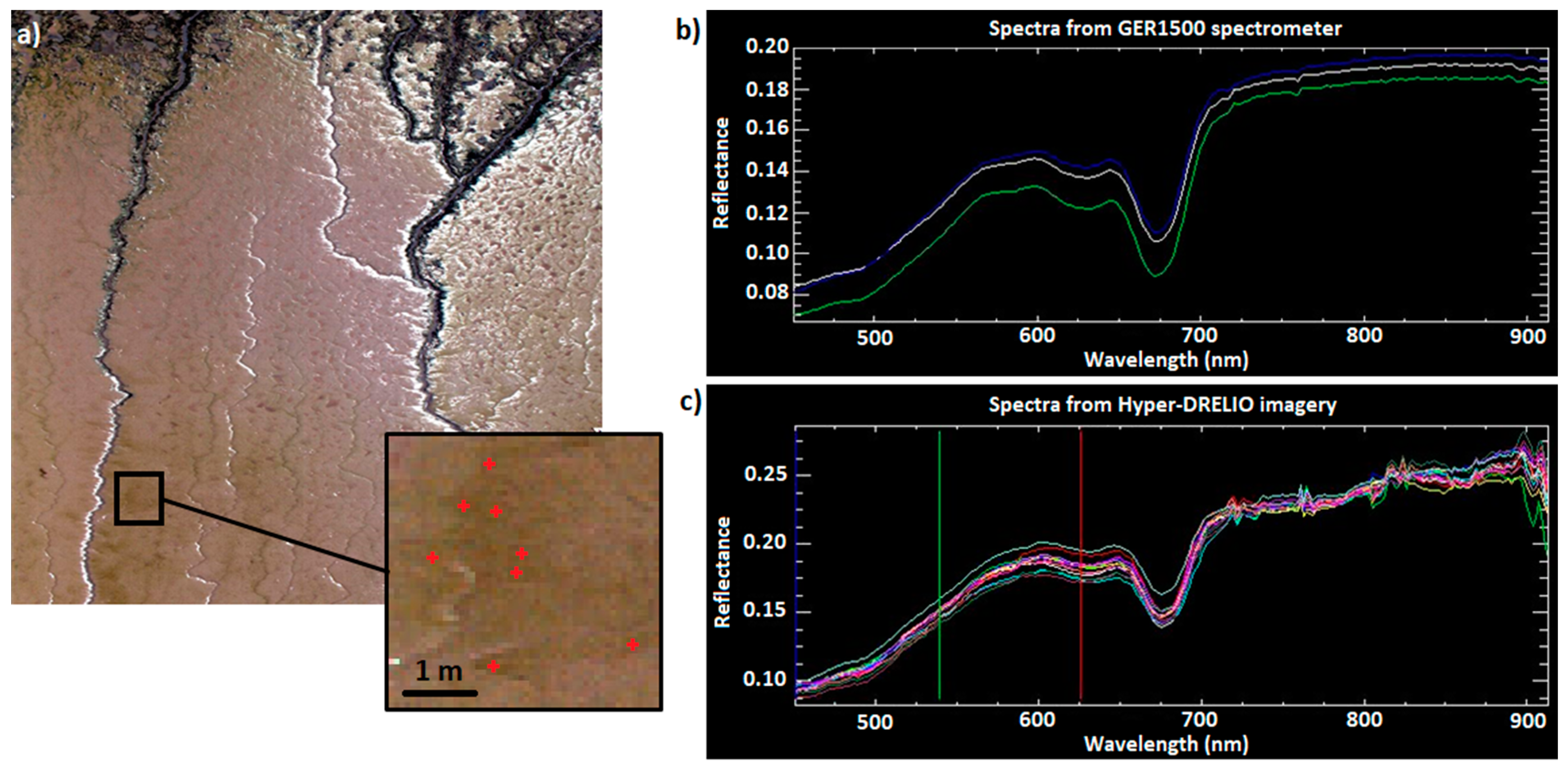
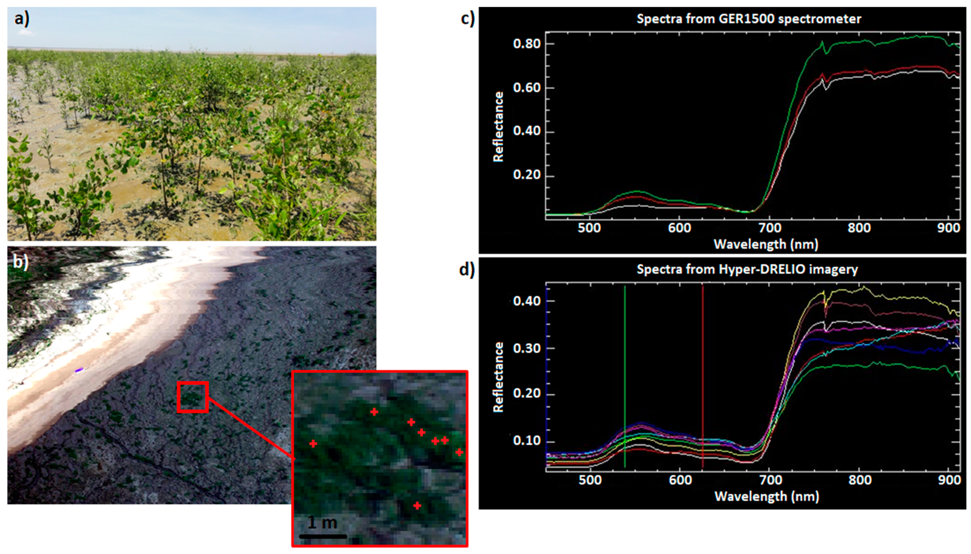
4.1. Comparison to Field Spectrometer

Hyper-DRELIO imagery and field spectrometer control measurements are not exactly synchronous (separated by a few minutes to an hour). In addition, since the field spectrometer measurements are performed from the fixed platform, they can be separated from the Hyper-DRELIO images by several tens of meters. Differences between the spectra may appear, depending on the type/concentration of the benthic biofilm, which is related to the tidal time or on local variations of the targeted materials (concentration, structure, spectral mixing, or surface orientation).

Figure 6 and Figure 7 show the spectra obtained over the sediment surface covered by benthic biofilm and over the pioneer mangroves, respectively. For a given class of targets, the characteristics of the spectra are globally similar between the field spectrometer and Hyper-DRELIO imagery, with local minima and maxima being clearly identifiable, both for the benthic biofilm and the pioneer mangroves. Thus, Hyper-DRELIO imagery succeeds in spatially capturing the spectral specificities of each target class. However, Hyper-DRELIO data are noisier for wavelengths higher than 800 nm. To evaluate the degree of similarity between the Hyper-DRELIO reflectance spectra and the field spectrometer reflectance spectra, we used a correlation coefficient to compare the reflectance levels and the spectral angle mapper (SAM) method [58]. The SAM “distance” assesses the similarity between the shape of two spectra by calculating the angle between these spectra and is, therefore, less sensitive to multiplicative noise. The smaller the SAM distance, the higher the similarity (two exactly similar spectra would have a zero SAM distance). We compare the mean value of three spectra measured by the field spectrometer (Figure 6b and Figure 7c) and the mean value of eight spectra extracted from Hyper-DRELIO images (Figure 6c and Figure 7d) for the two biota. Above the benthic biofilm, a SAM distance of 0.039 and a correlation coefficient of 0.96 were found. Above the pioneer mangrove, the SAM distance was 0.159 and the correlation coefficient was 0.97.

With a small pixel size, the probability of capturing different class of targets in a pixel is limited. Nevertheless, a very high spatial resolution also captures some complexities that are not visible at lower resolutions, such as the structure of the foliage. Figure 6c and Figure 7d show a disparity between the spectra extracted from Hyper-DRELIO imagery (mean standard deviation of 0.004 for the biofilm, and 0.061 for the mangrove, respectively). In the visible spectrum, the spectral signature is mainly influenced by pigment composition. In NIR (near infrared), the spectrum is rather influenced by the structure and water content of the target. That explains the higher disparity (particularly in NIR) obtained among mangrove spectra, extracted from Hyper-DRELIO imagery.

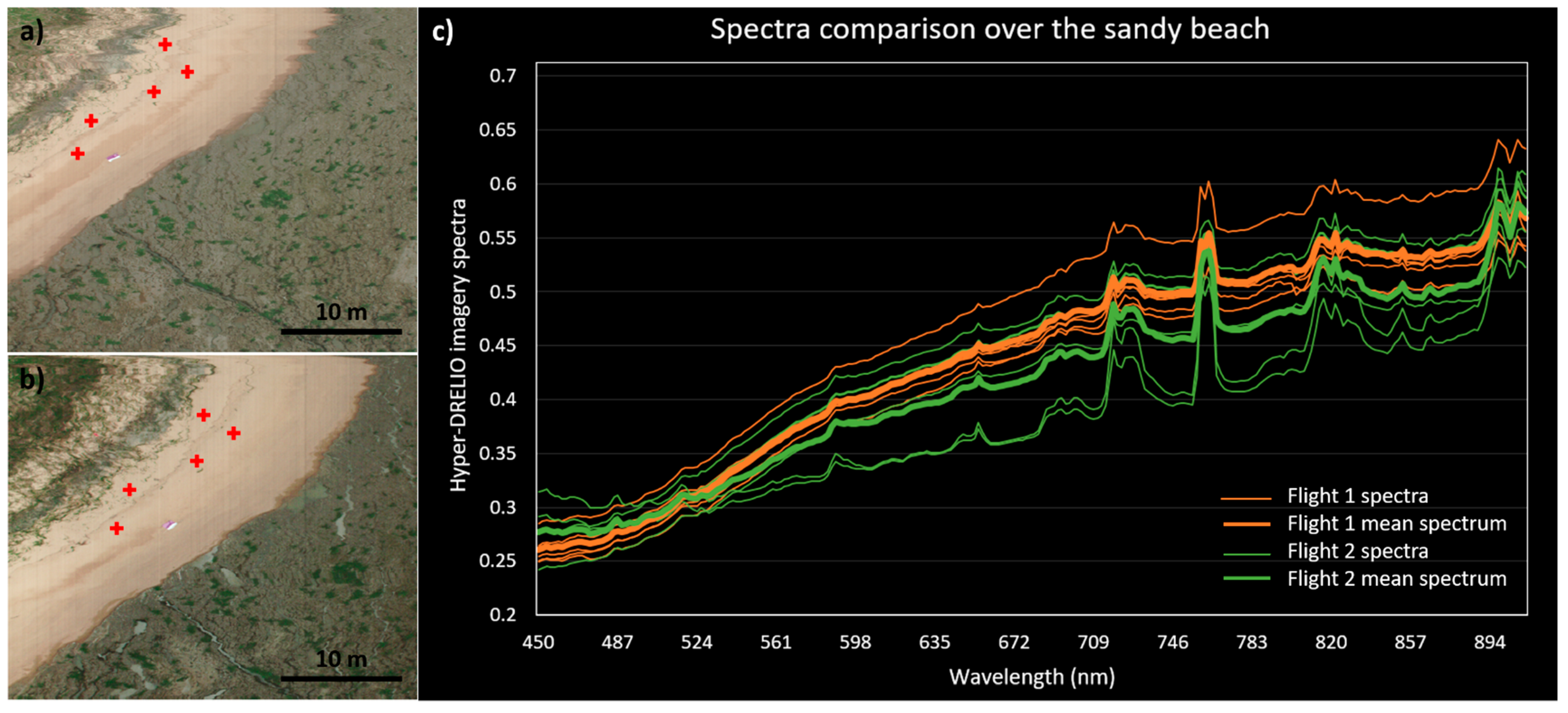
4.2. Relative Comparison over the Sandy Beach

As the flights were conducted at different times of the day, one way of checking the effectiveness of the radiometric corrections is to compare the spectra acquired several hours apart over the same substrate. Since the surface texture of the mudflat may change during the tidal cycle because of biofilm development, desiccation, and/or bioturbation processes, the part of the study area assumed to change the least over time was the upper sandy beach.

Two sets of five spectra were extracted on the supra-tidal part of the beach for the flight on 12 September 2018 at 11:30 (Flight 1) and for the flight on 12 September 2018 at 13:30 (Flight 2). From these spectra (Figure 8), the intra-set variability (for the same flight) was evaluated from the standard deviation (averaged over all wavelengths). For the spectra of Flight 1 (respectively, Flight 2), the standard deviation was 0.024 (or 5.48%), respectively, 0.037 (or 8.81%) for Flight 2. The quality of the radiometric corrections was assessed by comparing the average spectra from the two data sets (Vol 1 and Vol 2). The average difference between these average spectra was 0.026 (or 5.64%). This deviation was considered satisfactory as it was of the same order of magnitude as the intra-set variability.

5. Discussion

As previously mentioned, the goal of this study was to propose an efficient and easily implemented method to perform radiometric corrections of UAV-borne hyperspectral imagery—without adding embedded sensors and with minimum equipment (i.e., only two Spectralon panels and a field spectrometer)—which is adequate for “hard-to-access” ecosystems, such as the huge intertidal mudbanks along the Amazon-influenced, northeast coast of South America. Smith and Milton [55] reported that the empirical line method allows the calibration of remotely sensed data to reflectance with errors of only a few percent. This efficiency was confirmed for our UAV data by the obtained SAM distances and correlation scores. Here, we calculated a higher SAM distance for the pioneer mangrove forest than for the benthic biofilm. This result is coherent with the higher diversity observed among the mangroves spectra (both with the field spectrometer and with the UAV-borne camera—Figure 7c,d). Indeed, point-wise measurement (with the field spectrometer) and very high spatial resolution hyperspectral images (with UAV-borne camera) reflect the complex morphology induced by the mangroves canopy. On the contrary, a slightly lower correlation coefficient was obtained for the benthic biofilm. This could be due to the higher disparity, both spatially and temporally, of the biofilm concentration at the sediment surface, alongside local changes in sediment elevation and bioturbation activities [37].

This method of radiometric corrections, especially the initial calibration step, can also be used to monitor the drift of the manufacturer’s calibration. As previously mentioned, Hyper-DRELIO data are noisier for wavelengths higher than 800 nm. Proctor and He [8] explained that this effect is common and is due to the combination of a sharp decrease of quantum efficiency in the NIR, the lower solar output in the NIR, and reduced sensitivity of the imager resulting in lower signal and greater noise. The proposed radiometric correction process relies on simplifying assumptions, which are likely to cause some errors. For instance, remaining noise can be due to DC, which has been considered steady here. Besides, as the “sun–target–sensor” geometry varies for all the pixels recorded by the camera, bidirectional reflectance effects can also influence the signal [33]. As mentioned by Garzonio et al. [34], light intensity could be optimized by placing neutral filters to avoid saturation for very high light intensities. Lastly, the proposed approach to take into account temporal variations of irradiance suits for the variations of ambient light but fails to take into account local effects, which are not captured by the field spectrometer above the 99% Spectralon panel. Therefore, some parts of the images can be affected by spatial changes in the illumination fields, due to isolated clouds or shadows originating from the geometrical configuration of the scene (e.g., presence of trees).

Moreover, as the Spectralons panels are of great importance in this method for radiometric corrections, the results would be sensitive to defects in Spectralon surfaces. For that matter, Bachmann et al. [48] mention that white Spectralon panels are subject to repeated handling and exposed to various environmental factors. Therefore, their calibration coefficients drift over time.

The methodology proposed can be extended to other types of areas, provided that topography-induced illumination differences are taken into account [59].

For now, we have not assessed the impact of platform vibrations on the radiometric and spectral stability of the hyperspectral camera (shift, band broadening, etc.). According to Garzonio et al. [34], however, the impact of platform mechanical vibrations would be almost insignificant in terms of band centre, width, and radiometric response.

Field access in the mangroves developing under Amazonian influence is particularly difficult. Thus, in this particular rapidly evolving ecosystem, future work should aim to assess the extent to which the very high spatial and spectral resolution provided by hyperspectral UAV can capture the biological complexity of the substrate. The good correlations found in this study between drone imagery after radiometric corrections and the in situ spectrometer measurements for the benthic biofilm and pioneer mangroves should allow simultaneous mapping of mangrove forests and benthic biofilm distribution at the mudbank scale, integrating small-scale heterogeneity, caused by the combined effects of geomorphology, tides, and biology (e.g., bioturbation). This method, tested in mangroves under limited human impacts, shows new possibilities for monitoring mangrove ecosystems facing different levels of pressure and subsequent alteration along the nearby coastline (Guyana and Surinam), as well as in other biogeographic regions with other mangrove species and dynamics.

6. Conclusions

Hyper-DRELIO allowed hyperspectral data to be collected above few hectares of mangrove forests and mudbanks in French Guiana, with both high spatial resolution and high spectral resolution in the VNIR domain. One of the main advantages of drones being their flexibility, the associated imagery calibration procedures have to be as simple as possible to keep the latter. This study proposes an easy, in situ radiometric calibration method, dedicated to drone-based hyperspectral surveys, without adding embedded sensors and with minimum equipment, using only two Spectralon (white and grey) and a ground spectrometer. The proposed procedure enables to calibrate the sensor, by correcting lining effects and transforming the raw relative DN generated by the hyperspectral camera into reflectance values standardized to in situ illumination conditions.

The radiometric corrections were applied to a small subset of a dataset collected above mudbanks colonised by benthic biofilm and a pioneer mangrove forest. Besides the fact that the shapes of spectra are globally consistent between the radiometrically corrected Hyper-DRELIO spectra and the in situ typical spectra, their degree of similarity was assessed using the SAM distance and correlation coefficient. SAM distance values of 0.039 above biofilm and 0.159 above pioneer mangrove forest, together with associated correlation coefficients (of 0.96 and 0.97, respectively), are greatly satisfying for substrate classification. Future work will consist of applying this method to the entire study area, in order to spatialize the results, and comparing hyperspectral and in situ data in order to obtain the finest possible classification of the various detectable elements.

References

1. Sandilyan, S.; Kathiresan, K. Mangrove Conservation: A Global Perspective. Biodivers. Conserv. 2012, 21, 3523–3542. [Google Scholar] [CrossRef]
2. Alongi, D.M. Mangrove Forests: Resilience, Protection from Tsunamis; and Responses to Global Climate Change. Estuar. Coast. Shelf Sci. 2008, 76, 1–13. [Google Scholar] [CrossRef]
3. Thomas, N.; Lucas, R.; Bunting, P.; Hardy, A.; Rosenqvist, A.; Simard, M. Distribution and Drivers of Global Mangrove Forest Change, 1996–2010. PLoS ONE 2017, 12, e0179302. [Google Scholar] [CrossRef] [PubMed] [Green Version]
4. Green, E.P.; Clark, C.D.; Mumby, P.J.; Edwards, A.J.; Ellis, A.C. Remote Sensing Techniques for Mangrove Mapping. Int. J. Remote Sens. 1998, 19, 935–956. [Google Scholar] [CrossRef]
5. Kuenzer, C.; Bluemel, A.; Gebhardt, S.; Quoc, T.V.; Dech, S. Remote Sensing of Mangrove Ecosystems: A Review. Remote Sens. 2011, 3, 878–928. [Google Scholar] [CrossRef] [Green Version]
6. Wang, L.; Jia, M.; Yin, D.; Tian, J. A Review of Remote Sensing for Mangrove Forests: 1956–2018. Remote Sens. Environ. 2019, 231, 111223. [Google Scholar] [CrossRef]
7. Schaepman, M.E.; Ustin, S.L.; Plaza, A.J.; Painter, T.H.; Verrelst, J.; Liang, S. Earth System Science Related Imaging Spectroscopy—An Assessment. Remote Sens. Environ. 2009, 113, 123–137. [Google Scholar] [CrossRef]
8. Proctor, C.; He, Y. Workflow for Building a Hyperspectral UAV: Challenges and Opportunities. ISPRS Ann. Photogramm. Remote Sens. Spat. Inf. Sci. 2009, XL-1/W4, 415–419. [Google Scholar] [CrossRef] [Green Version]
9. Launeau, P.; Kassouk, Z.; Debaine, F.; Roy, R.; Mestayer, P.G.; Boulet, C.; Rouaud, J.-M.; Giraud, M. Airborne Hyperspectral Mapping of Trees in an Urban Area. Int. J. Remote Sens. 2017, 38, 1277–1311. [Google Scholar] [CrossRef]
10. Kruse, F.A.; Boardman, J.W.; Huntington, J.F. Comparison of Airborne Hyperspectral Data and Eo-1 Hyperion for Mineral Mapping. IEEE Trans. Geosci. Remote Sens. 2003, 41, 1388–1400. [Google Scholar] [CrossRef] [Green Version]
11. Burai, P.; Deák, B.; Valkó, O.; Tomor, T. Classification of Herbaceous Vegetation Using Airborne Hyperspectral Imagery. Remote Sens. 2015, 7, 2046–2066. [Google Scholar] [CrossRef] [Green Version]
12. Kamal, M.; Phinn, S. Hyperspectral data for mangrove species mapping: A comparison of pixel-based and object-based approach. Remote Sens. 2011, 3, 2222–2242. [Google Scholar] [CrossRef] [Green Version]
13. Peerbhay, K.Y.; Mutanga, O.; Ismail, R. Commercial tree species discrimination using airborne AISA Eagle hyperspectral imagery and partial least squares discriminant analysis (PLS-DA) in KwaZulu–Natal, South Africa. ISPRS J. Photogramm. Remote Sens. 2013, 79, 19–28. [Google Scholar] [CrossRef]
14. Richter, R.; Reu, B.; Wirth, C.; Doktor, D.; Vohland, M. The use of airborne hyperspectral data for tree species classification in a species-rich Central European forest area. Int. J. Appl. Earth Obs. Geoinf. 2016, 52, 464–474. [Google Scholar] [CrossRef]
15. Yang, C.; Everitt, J.H.; Fletcher, R.S.; Jensen, R.R.; Mausel, P.W. Evaluating AISA + Hyperspectral Imagery for Mapping Black Mangrove along the South Texas Gulf Coast. Photogramm. Eng. Remote Sens. 2009, 4, 425–435. [Google Scholar] [CrossRef] [Green Version]
16. Chaube, N.R.; Lele, N.; Misra, A.; Murthy, T.; Manna, S.; Hazra, S.; Panda, M.; Samal, R.N. Mangrove species discrimination and health assessment using AVIRIS-NG hyperspectral data. Curr. Sci. 2019, 116, 1136. [Google Scholar] [CrossRef]
17. Hati, J.P.; Goswami, S.; Samanta, S.; Pramanick, N.; Majumdar, S.D.; Chaube, N.R.; Misra, A.; Hazra, S. Estimation of vegetation stress in the mangrove forest using AVIRIS-NG airborne hyperspectral data. Model. Earth Syst. Environ. 2021, 7, 1877–1889. [Google Scholar] [CrossRef]
18. Hati, J.P.; Samanta, S.; Chaube, N.R.; Misra, A.; Giri, S.; Pramanick, N.; Gupta, K.; Majumdar, S.D.; Chanda, A.; Mukhopadhyay, A.; et al. Mangrove classification using airborne hyperspectral AVIRIS-NG and comparing with other spaceborne hyperspectral and multispectral data. Egypt. J. Remote Sens. Space Sci. 2021, 24, 273–281. [Google Scholar] [CrossRef]
19. Jiang, Y.; Zhang, L.; Yan, M.; Qi, J.; Fu, T.; Fan, S.; Chen, B. High-Resolution Mangrove Forests Classification with Machine Learning Using Worldview and UAV Hyperspectral Data. Remote Sens. 2021, 13, 1529. [Google Scholar] [CrossRef]
20. Liu, L.; Coops, N.C.; Aven, N.W.; Pang, Y. Mapping urban tree species using integrated airborne hyperspectral and LiDAR remote sensing data. Remote Sens. Environ. 2017, 200, 170–182. [Google Scholar] [CrossRef]
21. Li, Q.; Wong, F.K.K.; Fung, T. Mapping multi-layered mangroves from multispectral, hyperspectral, and LiDAR data. Remote Sens. Environ. 2021, 258, 112403. [Google Scholar] [CrossRef]
22. Stuart, M.B.; McGonigle, A.J.S.; Willmott, J.R. Hyperspectral Imaging in Environmental Monitoring: A Review of Recent Developments and Technological Advances in Compact Field Deployable Systems. Sensors 2019, 19, 3071. [Google Scholar] [CrossRef] [PubMed] [Green Version]
23. Cao, J.; Leng, W.; Liu, K.; Liu, L.; He, Z.; Zhu, Y. Object-based mangrove species classification using unmanned aerial vehicle hyperspectral images and digital surface models. Remote Sens. 2018, 10, 89. [Google Scholar] [CrossRef] [Green Version]
24. Liu, X.; Wang, L. Feasibility of using consumer-grade unmanned aerial vehicles to estimate leaf area index in Mangrove forest. Remote Sens. Lett. 2018, 9, 1040–1049. [Google Scholar] [CrossRef]
25. Jaakkola, A.; Hyyppä, J.; Kukko, A.; Yu, X.; Kaartinen, H.; Lehtomäki, M.; Lin, Y. A low-cost multi-sensoral mobile mapping system and its feasibility for tree measurements. ISPRS J. Photogramm. Remote Sens. 2010, 65, 514–522. [Google Scholar] [CrossRef]
26. Kosugi, Y.; Mukoyama, S.; Takabayashi, Y.; Uto, K.; Oda, K.; Saito, G. Low-altitude hyperspectral observation of paddy using radio-controlled helicopter. In Proceedings of the IEEE International Geoscience and Remote Sensing Symposium (IGARSS), Vancouver, BC, Canada, 24–29 July 2011; pp. 1748–1751. [Google Scholar]
27. Hruska, R.; Mitchell, J.; Anderson, M.; Glenn, N.F. Radiometric and Geometric Analysis of Hyperspectral Imagery Acquired from an Unmanned Aerial Vehicle. Remote Sens. 2012, 4, 2736–2752. [Google Scholar] [CrossRef] [Green Version]
28. Gallay, M.; Eck, C.; Zgraggen, C.; Kaňuk, J.; Dvorný, E. High Resolution Airbone Laser Scanning and Hyperspectral Imaging with a small UAV platform. ISPRS Ann. Photogramm. Remote Sens. Spat. Inf. Sci. 2016, XLI-B1, 823–827. [Google Scholar] [CrossRef] [Green Version]
29. Lucieer, A.; Malenovský, Z.; Veness, T.; Wallace, L. HyperUAS—Imaging Spectroscopy from a Multirotor Unmanned Aircraft System. J. Field Rob. 2014, 31, 571–590. [Google Scholar] [CrossRef] [Green Version]
30. Jaud, M.; Le Dantec, N.; Ammann, J.; Grandjean, P.; Constantin, D.; Akhtman, Y.; Barbieux, K.; Allemand, P.; Delacourt, C.; Merminod, B. Direct Georeferencing of a Pushbroom, Lightweight Hyperspectral System for Mini-UAV Applications. Remote Sens. 2018, 10, 204. [Google Scholar] [CrossRef] [Green Version]
31. Oliveira, R.A.; Tommaselli, A.M.G.; Honkavaara, E. Generating a Hyperspectral Digital Surface Model Using a Hyperspectral 2D Frame Camera. ISPRS J. Photogramm. Remote Sens. 2019, 147, 345–360. [Google Scholar] [CrossRef]
32. Saari, H.; Pölönen, I.; Salo, H.; Honkavaara, E.; Hakala, T.; Holmlund, C.; Mäkynen, J.; Mannila, R.; Antila, T.; Akujärvi, A. Miniaturized hyperspectral imager calibration and uav flight campaigns. In Proceedings of the SPIE, Sensors, Systems, and Next-Generation Satellites XVII, Dresden, Germany, 24 October 2013; Volume 8889. [Google Scholar] [CrossRef]
33. Aasen, H.; Burkart, A.; Bolten, A.; Bareth, G. Generating 3D Hyperspectral Information with Lightweight UAV Snapshot Cameras for Vegetation Monitoring: From Camera Calibration to Quality Assurance. ISPRS J. Photogramm. Remote Sens. 2015, 108, 245–259. [Google Scholar] [CrossRef]
34. Garzonio, R.; Di Mauro, B.; Colombo, R.; Cogliati, S. Surface Reflectance and Sun-Induced Fluorescence Spectroscopy Measurements Using a Small Hyperspectral UAS. Remote Sens. 2017, 9, 472. [Google Scholar] [CrossRef] [Green Version]
35. Burkart, A.; Cogliati, S.; Schickling, A.; Rascher, U. A Novel UAV-Based Ultra-Light Weight Spectrometer for Field Spectroscopy. IEEE Sens. J. 2014, 14, 62–67. [Google Scholar] [CrossRef]
36. Jaud, M.; Grasso, F.; Le Dantec, N.; Verney, R.; Delacourt, C.; Ammann, J.; Deloffre, J.; Grandjean, P. Potential of UAVs for Monitoring Mudflat Morphodynamics (Application to the Seine Estuary, France). ISPRS Int. J. Geoinf. 2016, 5, 50. [Google Scholar] [CrossRef] [Green Version]
37. Brunier, G.; Michaud, E.; Fleury, J.; Anthony, E.J.; Morvan, S.; Gardel, A. Assessing the relationships between macro-faunal burrowing activity and mudflat geomorphology from UAV-based Structure-from-Motion photogrammetry. Remote Sens. Environ. 2020, 241, 111717. [Google Scholar] [CrossRef]
38. Jolivet, M.; Anthony, E.J.; Gardel, A.; Brunier, G. Multi-Decadal to Short-Term Beach and Shoreline Mobility in a Complex River-Mouth Environment Affected by Mud From the Amazon. Front. Earth Sci. 2019, 7, 187. [Google Scholar] [CrossRef] [Green Version]
39. Anthony, E.J.; Gratiot, N. Coastal Engineering and Large-Scale Mangrove Destruction in Guyana; South America: Averting an Environmental Catastrophe in the Making. Ecol. Eng. 2012, 47, 268–273. [Google Scholar] [CrossRef]
40. Fromard, F.; Puig, H.; Mougin, E.; Marty, G.; Betoulle, J.L.; Cadamuro, L. Structure, above-ground biomass and dynamics of mangrove ecosystems: New data from French Guiana. Oecologia 1998, 115, 39–53. [Google Scholar] [CrossRef]
41. Gardel, A.; Gensac, E.; Anthony, E.; Lesourd, S.; Loisel, H.; Marin, D. Wave-formed mud bars: Their morphodynamics and role in opportunistic mangrove colonization. J. Coast. Res. 2011, Special Issue 64, 384–387. [Google Scholar]
42. Aschenbroich, A.; Michaud, E.; Stieglitz, T.; Fromard, F.; Gardel, A.; Tavares, M.; Thouzeau, G. Brachyuran crab community structure and associated sediment reworking activities in pioneer and young mangroves of French Guiana, South America. Estuar. Coast. Shelf Sci. 2016, 182, 60–71. [Google Scholar] [CrossRef] [Green Version]
43. Aller, R.C.; Blair, N.E. Carbon Remineralization in the Amazon–Guianas Tropical Mobile Mudbelt: A Sedimentary Incinerator. Cont. Shelf Res. 2006, 26, 2241–2259. [Google Scholar] [CrossRef]
44. Gontharet, S.; Mathieu, O.; Lévêque, J.; Milloux, M.-J.; Lesourd, S.; Philippe, S.; Caillaud, J.; Gardel, A.; Sarrazin, M.; Proisy, C. Distribution and Sources of Bulk Organic Matter (OM) on a Tropical Intertidal Mud Bank in French Guiana from Elemental and Isotopic Proxies. Chem. Geol. 2014, 376, 1–10. [Google Scholar] [CrossRef]
45. Ray, R.; Michaud, E.; Aller, R.; Vantrepotte, V.; Gleixner, G.; Walcker, R.; Devesa, J.; Le Goff, M.; Morvan, S.; Thouzeau, G. The sources and distribution of carbon (DOC, POC, DIC) in a mangrove dominated estuary (French Guiana, South America). Biogeochemistry 2018, 138, 297–321. [Google Scholar] [CrossRef]
46. Ray, R.; Thouzeau, G.; Walcker, R.; Vantrepotte, V.; Gleixner, G.; Morvan, S.; Devesa, J.; Michaud, E. Mangrove-Derived Organic and Inorganic Carbon Exchanges Between the Sinnamary Estuarine System (French Guiana, South America) and Atlantic Ocean. J. Geophys. Res. Biogeosci. 2020, 125, e2020JG005739. [Google Scholar] [CrossRef]
47. Brunier, G.; Anthony, E.J.; Gratiot, N.; Gardel, A. Exceptional Rates and Mechanisms of Muddy Shoreline Retreat Following Mangrove Removal. Earth Surf. Process. Landf. 2019, 44, 1559–1571. [Google Scholar] [CrossRef]
48. Bachmann, C.M.; Montes, M.J.; Parrish, C.E.; Fusina, R.A.; Nichols, C.R.; Li, R.-R.; Hallenborg, E.; Jones, C.A.; Lee, K.; Sellars, J.; et al. A Dual-Spectrometer Approach to Reflectance Measurements under Sub-Optimal Sky Conditions. Opt. Express 2012, 20, 8959. [Google Scholar] [CrossRef]
49. Kazemipour, F.; Méléder, V.; Launeau, P. Optical Properties of Microphytobenthic Biofilms (MPBOM): Biomass Retrieval Implication. J. Quant. Spectrosc. Radiat. Transf. 2011, 112, 131–s142. [Google Scholar] [CrossRef]
50. Launeau, P.; Méléder, V.; Verpoorter, C.; Barillé, L.; Kazemipour-Ricci, F.; Giraud, M.; Jesus, B.; Le Menn, E. Microphytobenthos Biomass and Diversity Mapping at Different Spatial Scales with a Hyperspectral Optical Model. Remote Sens. 2018, 10, 716. [Google Scholar] [CrossRef] [Green Version]
51. Cho, M.A.; Skidmore, A.K. A New Technique for Extracting the Red Edge Position from Hyperspectral Data: The Linear Extrapolation Method. Remote Sens. Environ. 2006, 101, 181–193. [Google Scholar] [CrossRef]
52. Alvarez-Vanhard, E.; Houet, T.; Mony, C.; Lecoq, L.; Corpetti, T. Can UAVs Fill the Gap between in Situ Surveys and Satellites for Habitat Mapping? Remote Sens. Environ. 2020, 243, 111780. [Google Scholar] [CrossRef]
53. Aasen, H.; Bendig, J.; Bolten, A.; Bennertz, S.; Willkomm, M.; Bareth, G. Introduction and Preliminary Results of a Calibration for Full-Frame Hyperspectral Cameras to Monitor Agricultural Crops with UAVs. ISPRS Ann. Photogramm. Remote Sens. Spat. Inf. Sci. 2014, XL-7, 1–8. [Google Scholar] [CrossRef] [Green Version]
54. Honkavaara, E.; Khoramshahi, E. Radiometric Correction of Close-Range Spectral Image Blocks Captured Using an Unmanned Aerial Vehicle with a Radiometric Block Adjustment. Remote Sens. 2018, 10, 256. [Google Scholar] [CrossRef] [Green Version]
55. Smith, G.M.; Milton, E.J. The Use of the Empirical Line Method to Calibrate Remotely Sensed Data to Reflectance. Int. J. Remote Sens. 1999, 20, 2653–2662. [Google Scholar] [CrossRef]
56. Näsi, R.; Honkavaara, E.; Blomqvist, M.; Lyytikäinen-Saarenmaa, P.; Hakala, T.; Viljanen, N.; Kantola, T.; Holopainen, M. Remote Sensing of Bark Beetle Damage in Urban Forests at Individual Tree Level Using a Novel Hyperspectral Camera from UAV and Aircraft. Urban. For. Urban. Green. 2018, 30, 72–83. [Google Scholar] [CrossRef]
57. Green, A.; Berman, M.; Switzer, P.; Craig, M.D. A transformation for ordering multispectral data in terms of image quality with implications for noise removal. IEEE Trans. Geosci. Remote Sens. 1988, 26, 65–74. [Google Scholar] [CrossRef] [Green Version]
58. Kruse, F.A.; Lefkoff, A.B.; Boardman, J.B.; Heidebrecht, K.B.; Shapiro, A.T.; Barloon, P.J.; Goetz, A.F.H. The Spectral Image Processing System (SIPS)—Interactive Visualization and Analysis of Imaging spectrometer data. Remote Sens. Environ. 1993, 44, 145–163. [Google Scholar] [CrossRef]
59. Lorenz, S.; Salehi, S.; Kirsch, M.; Zimmermann, R.; Unger, G.; Vest Sørensen, E.; Gloaguen, R. Radiometric Correction and 3D Integration of Long-Range Ground-Based Hyperspectral Imagery for Mineral Exploration of Vertical Outcrops. Remote Sens. 2018, 10, 176. [Google Scholar] [CrossRef] [Green Version]
Figure 1. (a) Localization of the study area in Awala-Yalimapo in the western part of French Guiana. (b) UAV flight plans above the study area, designed to capture the various mud facies (from bare mud to mangrove stages). (c) Diagram of a survey setup and the physical variables to be measured.
Remotesensing 13 04792 g001
Figure 2. (a,b) Hyper-DRELIO (Hyperspectral DRone for Environmental and LIttoral Observations) platform, unmanned aerial vehicle (UAV) for hyperspectral imagery. IMU: inertial motion unit; RTK GNSS: real time kinematic global navigation satellite system. (c) White Spectralon panel (reflectivity: 99%). (d) Grey Spectralon panel (reflectivity: 20%).
Remotesensing 13 04792 g002
Figure 3. Processing steps performed for radiometric corrections (“i” is the index of the pixel along the sensor array, in the across-track spatial dimension).
Remotesensing 13 04792 g003
Figure 4. Hyperspectral lines collected above the white Spectralon by the hyperspectral camera before (a,c) and after (b,d) calibration. (a,b) represent, in natural colors, the hyperspectral lines collected by the camera; (c,d) represent the values of digital number (DN) (c) and radiance (d) along the sensor line for each spectral band (in colors).
Remotesensing 13 04792 g004
Figure 5. (a) Field spectrometer (GER 1500) measuring the irradiance variability above the white Spectralon. (b) Example of variability of the spectra measured by the field spectrometer during a flight. (c) Example of the τ coefficient interpolated (green line) from the percentage of irradiance variations measured (red dots) during the flight.
Remotesensing 13 04792 g005
Figure 6. Spectra comparison above the benthic biofilm. (a) Biofilm patch on the Hyper-DRELIO image (in natural colours) where the spectra are pointed (red crosses). The image was acquired on 2018-09-12 at 13:15. (b) Biofilm spectra measured by GER1500 spectrometer. (c) Biofilm spectra extracted from Hyper-DRELIO imagery (mean standard deviation between the reflectance spectra: 0.004).
Remotesensing 13 04792 g006
Figure 7. Spectra comparison above the pioneer mangroves. (a) Aerial oblique photograph of the pioneer mangroves. (b) Mangrove patch on the Hyper-DRELIO image (in natural colours) where the spectra are pointed (red crosses). The image was acquired on 12 September 2018 at 11:08. (c) Mangrove spectra measured by GER1500 spectrometer. (d) Mangrove spectra extracted from Hyper-DRELIO imagery (mean standard deviation between the reflectance spectra: 0.061).
Remotesensing 13 04792 g007
Figure 8. Spectra comparison above the supra-tidal sandy beach. (a,b) Sandy beach on the Hyper-DRELIO images (in natural colours) where the spectra are pointed (red crosses). The images were acquired on 12 September 2018 at 11:08 (Flight 1) (a) and on 12 September 2018 at 13:14 (Flight 2) (b). (c) Sand spectra extracted from Hyper-DRELIO imagery for Flight 1 (orange colour) and Flight 2 (green colour). The mean spectrum for each data set is depicted in bold.
Remotesensing 13 04792 g008
Publisher’s Note: MDPI stays neutral with regard to jurisdictional claims in published maps and institutional affiliations.