Semi-Automatic Generation of Training Samples for Detecting Renewable Energy Plants in High-Resolution Aerial Images

Abstract

Deep learning (DL)—in particular convolutional neural networks (CNN)—methods are widely spread in object detection and recognition of remote sensing images. In the domain of DL, there is a need for large numbers of training samples. These samples are mostly generated based on manual identification. Identifying and labelling these objects is very time-consuming. The developed approach proposes a partially automated procedure for the sample creation and avoids manual labelling of rooftop photovoltaic (PV) systems. By combining address data of existing rooftop PV systems from the German Plant Register, the Georeferenced Address Data and the Official House Surroundings Germany, a partially automated generation of training samples is achieved. Using a selection of 100,000 automatically generated samples, a network using a RetinaNet-based architecture combining ResNet101, a feature pyramid network, a classification and a regression network is trained, applied on a large area and post-filtered by intersection with additional automatically identified locations of existing rooftop PV systems. Based on a proof-of-concept application, a second network is trained with the filtered selection of approximately 51,000 training samples. In two independent test applications using high-resolution aerial images of Saarland in Germany, buildings with PV systems are detected with a precision of at least 92.77 and a recall of 84.47.

1. Introduction

Machine learning (ML) methods have already proven to be helpful for localizing objects in the past. This offers the possibility to recognize objects in aerial images and thus to identify the locations of renewable power generators such as PV roof-mounted systems for energy system analysis. Several papers on the detection of PV systems have already been published over the last years [1,2,3,4,5,6,7]. In general, all authors used supervised learning methods, where datasets are created initially by labelling a huge number of objects of the given class. The number of training samples used for the detection of PV systems increased steadily with the development of the methodologies. For example, [2] uses over 2700 images containing PV systems, [5] more than 50,000 and [6] up to 70,673 labelled images. The creation of such large amounts of training data is very time- and cost-intensive [8,9]. To avoid the tedious preparation of data, only a few approaches have been presented. An example of the automated creation of training data using different data sources such as OpenStreetMap (OSM) and automatic information indexes referring to buildings, shadow, vegetation, and water has already shown good results in the task of image classification using maximum likelihood classification (MLC), multilayer perceptron (MLP), support vector machine (SVM), and random forest (RF) classifier. Not included in that study are approaches using modern CNN networks [10]. During the research of the present work, no approaches of an application of CNN classifiers for object detection using automatically generated training data could be found. Therefore, the present work ties in with the idea of automatic generation of training samples. Since deep learning networks such as CNN networks in particular are capable of producing reliable results on a growing base of training data, this paper relies on them. Due to the enormous costs and the unpredictable systematic bias of expert training, the semi-automatic acquisition of labelled training samples seems to be a suitable basis for efficient CNN classification.

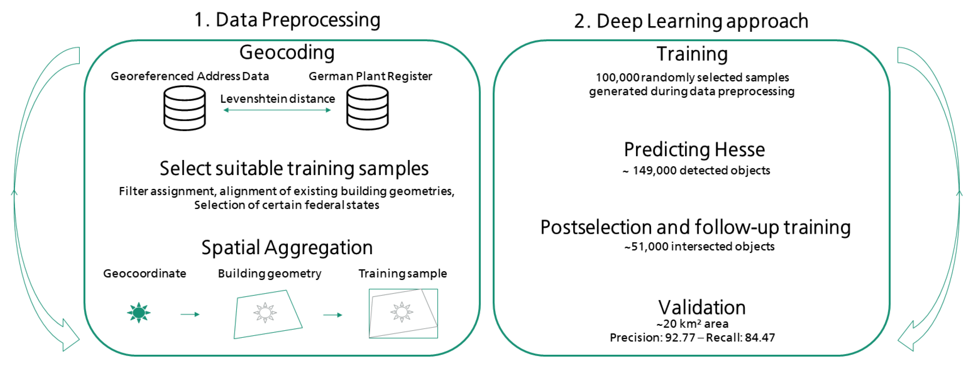
In this study, an operational semi-automatic workflow as shown in Figure 1 is developed by using an automated matching of location data from the German PV Plant Register and the Georeferenced Address Data first generate geocoordinates of existing plants. After selecting suitable training samples, the coordinates are aggregated by area using the Official House Surroundings Germany dataset. Subsequently, these marked areas are used as training samples for a CNN-based object detector. Through a pre-application to the territory of the German state of Hesse and an automated matching with geocoded plants, the objects are postfiltered and used for a follow-up training. Finally, the object detector is validated in a proof-of-concept study.

2. Materials

2.1. Georeferenced Address Data

The Georeferenced Address Data (GA) dataset provided by the Federal Agency for Cartography and Geodesy (BKG) contains completed and cleaned addresses, georeferencing coordinates, and a quality key for georeferenced building addresses at a uniform level of actuality for the federal territory of Germany. It is a summary of the Official House Coordinates of Germany of the land surveying administrations of the federal states and is supplemented at the BKG by addresses from the address dataset of Deutsche Post Direkt GmbH. The GA comprises about 22.6 million data records, proportionately about 730,000 data records from Deutsche Post [11].

2.2. Official House Surroundings Germany

The dataset published by the BKG summarizes the Official House Surroundings Germany (HU-DE) of the Central Office House Coordinates and House Surroundings of the surveying and cadastral administrations of the federal states and contains georeferenced house surround polygons of building ground plans of the Automated Real Estate Map [12].

2.3. German Plant Register

The German Plant Register was maintained by the Federal Network Agency for the German electricity and gas markets until 2019. The register contains information on players and installations in the grid-based energy supply market. In addition to registered power generation units, addresses, and power values for PV systems installed in Germany are listed, among other variables. In this work, these form the basis for determining the locations of existing PV systems.

2.4. Digital Orthophotos

The product of the Digital Orthophotos (DOP) of Germany [13] consists of georeferenced, differentially rectified aerial images of the surveying administrations of the federal states. They are true-to-scale raster data of photographic images of the earth’s surface, limited to the territory of the Federal Republic of Germany. In the present work the DOP with a ground resolution of 20 cm are used. They are available as tiles with a resolution of 5000 × 5000 pixels and a positional accuracy of ±0.4 m standard deviation. Thus, an area of 1000 × 1000 m is displayed per image. The product includes colour images (RGB) as well as infrared images and colour infrared (CIR) images. The present work uses the false colour composite CIR images, combining the infrared channel with the two visible colour or channels red and green.

3. Methodology

3.1. Data Preprocessing

To generate training samples, the address data of existing PV rooftop systems from the Plant Register were first geocoded by mapping these address data to geocoordinates from the GA. A method called Levenshtein distance was used for this purpose [14]. In contrast to exact mapping algorithms, this technique allows an approximation to two strings [15]. The minimum distance $D_{i,j}$ was calculated in a $m\times n$ matrix where each original address string from the Plant Register $X=x_1,x_2,\cdots x_m$ was adapted sign-by-sign to match the target address string from the GA addresses $Y=y_1,y_2,\cdots y_n$. Three different possible operations, such as insert $D_{i,j-1}$, delete $D_{i-1,j}$, and substitute $D_{i-1,j-1}$ can be used to convert each cell ($i,j$), which represents the distance between the original substring $X_i^1=x_1,x_2,\cdots x_i$ and the target substring $Y_j^1=y_1,y_2,\cdots y_j$ [16].

$$D_{i,j}=min\left\{\begin{array}{l}{D}_{i-1,j-1}+0if{X}_{i-1}=Y_{j-1}\hfill \\ D_{i,j-1}+1\left(insert\right)\hfill \\ D_{i-1,j}+4\left(delete\right)\hfill \\ D_{i-1,j-1}+10\left(substitute\right)\hfill \end{array}\right.$$

(1)

The minimum number of operations was added up according to their cost (insert $+1$, delete $+4$, replace $+10$), so that the result was a weighted sum of operations that have to be performed to find the best match between the respective strings. The weighted sum could be used as a quality measure for the match and was exploited and filtered so that only geocoded PV addresses with a difference of 0, i.e., ideal matches, were used for further labelling. The assigned geocoordinates of the existing PV rooftop systems could then be provided with polygons of the HU-DE using a spatial intersection. In addition, the plants were filtered by a quality key of HU-DE, which ensured that the coordinates used lay safely within the recorded building geometries. Since the CNN architecture provides rectangular bounding boxes, the polygons were abstracted to rectangles in a further step. In order not to exceed the maximum tile size of the selected Backbone ResNet101 (768–1024 pixels), the original DOP tiles were divided into subareas of 1000 × 1000 pixels, each 200 × 200 m. It should be emphasized that the buildings with PV systems used as training samples always represented only a very small proportion of the image sections. Image sections without assignment to a class were interpreted as background class.

3.2. Deep Learning Approach

3.2.1. CNN Architecture

The CNN network was based on the architecture called RetinaNet [17], combining the deep residual neural network ResNet101 [18], a feature pyramid network (FPN) [19] following previous object detectors such as “faster R-CNN” [20], and two task-specific classification and regression subnetworks. RetinaNet was used because, when compared by the COCO benchmark, it outperformed all previous one- and two-stage detectors, including the winners of the COCO 2016 competition, in terms of prediction accuracy relative to speed. The classification subnetwork performs object classification at the output of the backbone network based on focal loss ($FL$). The focal loss is designed to train extremely unevenly distributed foreground and background classes. Based on the cross entropy loss for binary classification it adds a weighting factor $\alpha \in [0,1]$ for class 1 and $1-\alpha$ for class $-1$ as well as a modulation factor ${(1-p_t)}^{\gamma }$ containing a tunable focusing parameter $\gamma \ge 0$, as shown in Equation (2) [17].

$$FL\left(p_t\right)=-{\alpha }_t{(1-p_t)}^{\gamma }log\left(p_t\right)$$

(2)

The parameters were set to $\alpha$ = 0.25, $\gamma$ = 2.0, p = 0.5, as ablation experiments achieved good results with this parameter combination. The regression subnetwork was implemented for regressive delineation of objects. The regression loss ($L_{loc}$) is based on the smooth L1 loss ($smoot{h}_{L_1}$) approach, originally designed as part of the Fast R-CNN network [20]. The regression loss was used to target the bounding box regression and was defined over a tuple for the ground-truth class u and v for the bounding box regression target $u,v=(v_x,v_y,v_w,v_h)$ and a predicted tuple for the class u with $t^u=(t_x^u,t_y^u,t_w^u,t_h^u)$ [20], adapted [17] and implemented in [21] as shown in Equations (3) and (4).

$$L_{loc}(t^u,v)=\sum _{i\in \{x,y,w,h\}}smoot{h}_{L_1}(t_i^u-v_i)$$

(3)

in which

$$smoot{h}_{L_1}\left(x\right)=\left\{\begin{array}{c}0.5*{(\sigma *x)}^{2}if\left|x\right|<1/{\sigma }^2\hfill \\ \left|x\right|-0.5/{\sigma }^{2}otherwise\hfill \end{array}\right.$$

(4)

The parameter $\sigma$ was set to 3.0. The regression targets were output as rectangles that were entirely within the images shown and could take given aspect ratios of 1:2, 1:1, and 2:1. The result in predictions can be at multiple levels of the network, since there are multiple output layers. Based on good performance from previous object detection tasks, ResNet101 with an image size of 768–1024 pixels was chosen as the backbone network [18,22,23]. Since it has been repeatedly shown that pretrained networks achieve good generalization more quickly, an already implemented, freely available ResNet101 was used, which had already been pretrained with 500 classes from the Open Image Dataset [21,24]. The learning rate started with 0.00001 and was reduced by factor 0.1 after 2 epochs during training without improvement, as measured by the values of total loss, which was calculated by summing up the $FL$ and the $L_{loc}$.

3.2.2. Training

The first training used 100,000 randomly selected, labelled images from the German states of Berlin, North Rhine-Westphalia and Thuringia as they were all generated automatically during the data preprocessing. The batch size was set to 100 and a termination criterion was selected so that the training was terminated if no progress was achieved as measured by the area under the precision–recall curve called average precision (AP) after 5 epochs. The validation dataset was prepared manually and contained images with 280 located PV systems. For this purpose, the selection of images was screened and the existing bounding boxes were supplemented or adjusted so that all validation images were fully equipped with bounding boxes of existing PV systems.

The Intersection over union (IoU) was first calculated by dividing the area overlap of detected objects and labelled objects by the total area of the two boxes. By classifying the results based on the threshold value of 0.5, we determined whether the detection matched the labelled object. If the IoU was higher than 0.5, the detection was considered as a true positive (TP). If it was lower, the detection was considered a false positive (FP). False negatives (FNs) referred to existing objects that were not recognized during prediction. True negatives (TNs) could also be considered a background class as they represented the image sections that did not belong to any class. As a result of the number of TP as well as FP and FN examples, the precision, recall, and the AP were calculated and are shown in

Table 1. The table summarizes the formulas of the evaluation. In addition to the precision and the recall, the average precision is presented.

	Formula
precision	$prec=\frac{TP}{TP+FP}$
recall	$rec=\frac{TP}{TP+FN}$
average precision	$AP={\int }_0^{1}Pr\left(Re\right)dRe$

.

3.2.3. Predicting Hesse

The trained model was applied to the area of the state of Hesse to ensure that none of the training data was reused for this initial test application. All detected plants with a threshold classification score of more than 0.3 were prepared as training examples for a follow-up training session. Doubly detected PV systems were reduced in a further step while the number of overlapping regression boxes was reduced based on the values of the score, so that only the boxes with the highest score remained.

3.2.4. Post Selection and Follow-Up Training

In a further step, the geocoded addresses with a PV system and objects resulting from the detection were compared. Since the automated generation of the training samples also generated erroneous bounding boxes, all objects in Hesse were marked where the centre of the detected objects lay within the building geometry of the geocoded addresses with a PV system. Furthermore, the existing bounding boxes were adjusted by adopting the boxes resulting from the detection as new bounding boxes. These marked objects were subsequently used for a follow-up training with the same architecture and parameters.

3.2.5. Validation

To assess the accuracy of the model, an independent test application was carried out using a selection of DOP from the federal state of Saarland in Germany. Here, 385 randomly drawn images used in a first test represented the overall coverage as far as possible. In addition, an artificial enrichment of 121 images was used in a second test leading to a disproportionate occurrence of PV systems. The following

Table 2. The table shows the number of images, the area covered by the images and the number of buildings used for validation.

	Random Images	Images with PV	Overall
images	385	121	506
covered area (km²)	15.4	4.84	20.24
buildings	2870	6475	9345

shows the numbers of images and the area covered by the images in km². Furthermore, the number of buildings recorded in the HU-DE within the test images are noted.

According to the HU-DE, there were a total of 9345 buildings in the test application on a total area of 20.24 km². Buildings without a PV system were subsequently summarized as background class TN. To get an overview of the output of the trained network, all images including the predictions of the test were displayed. A manual check of all outputs was then carried out to examine the extent to which repeated patterns occurred in the detection of the objects. The precision and recall were then calculated.

4. Results

This section presents the results of the proof-of-concept. First, the results of the training with automatically generated samples from the federal states of Berlin, North Rhine-Westphalia, and Thuringia are shown. The subsequent filtering from the prediction and geocoded systems of Hesse as well as the follow-up training are presented in the second part. Finally, the results of the independent validation in the federal state of Saarland are presented.

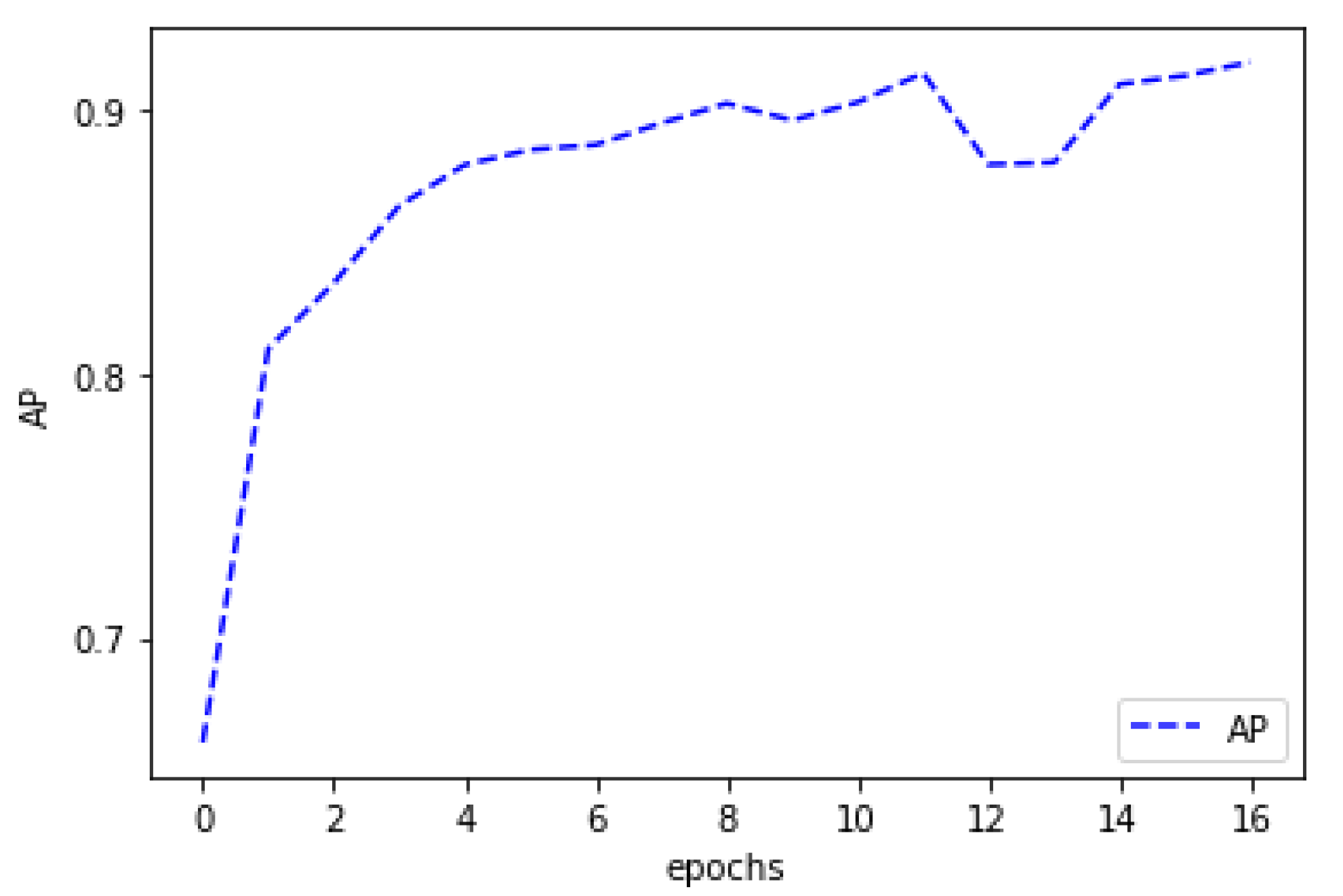
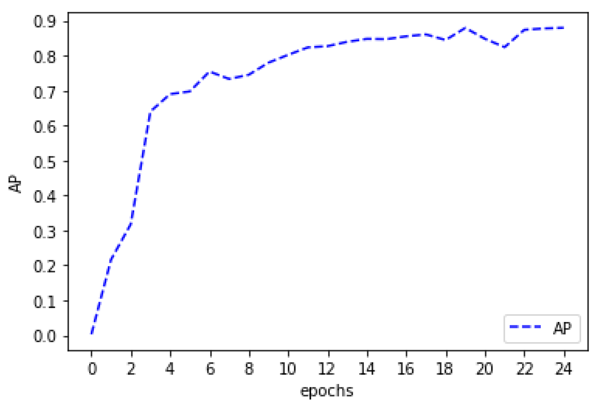
During the first training, the regression loss reaches a minimum of 0.19. The classification loss drops to a minimum of 0.66 (Figure 2). The calculated AP is 87.95% after the 24 epoch Figure 3.

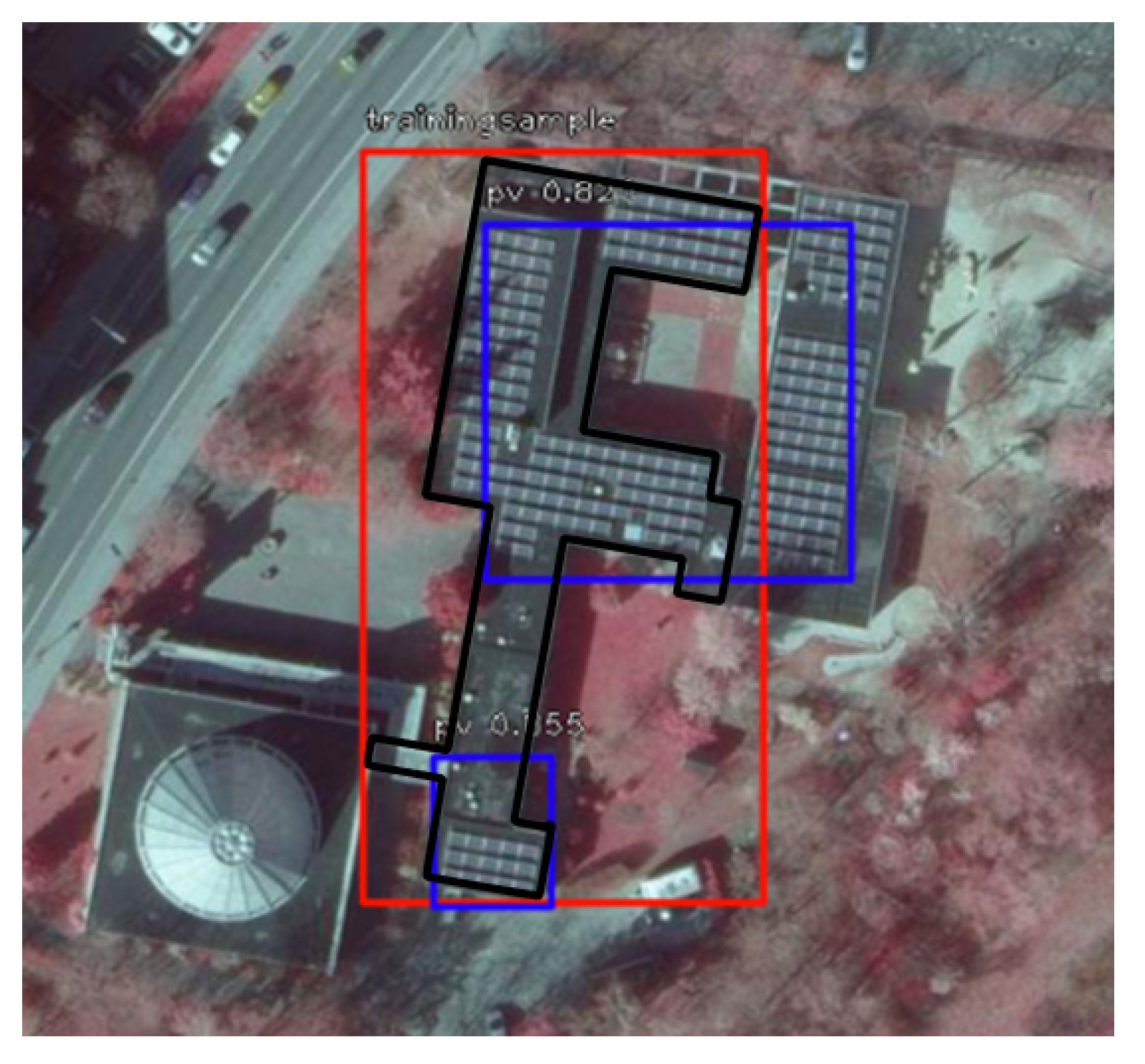
A total of 148,898 objects were detected during the prediction of the entire area of Hesse. The comparison of the overlap of the detected objects and the automatically generated geometries of the preprocessing resulted in 50,875 PV system locations. The existing bounding boxes (Figure 4, red) were adjusted by adopting the boxes resulting from the detection (Figure 4, blue) as new bounding boxes. These marked objects were subsequently used for a follow-up training with the same architecture and parameters.

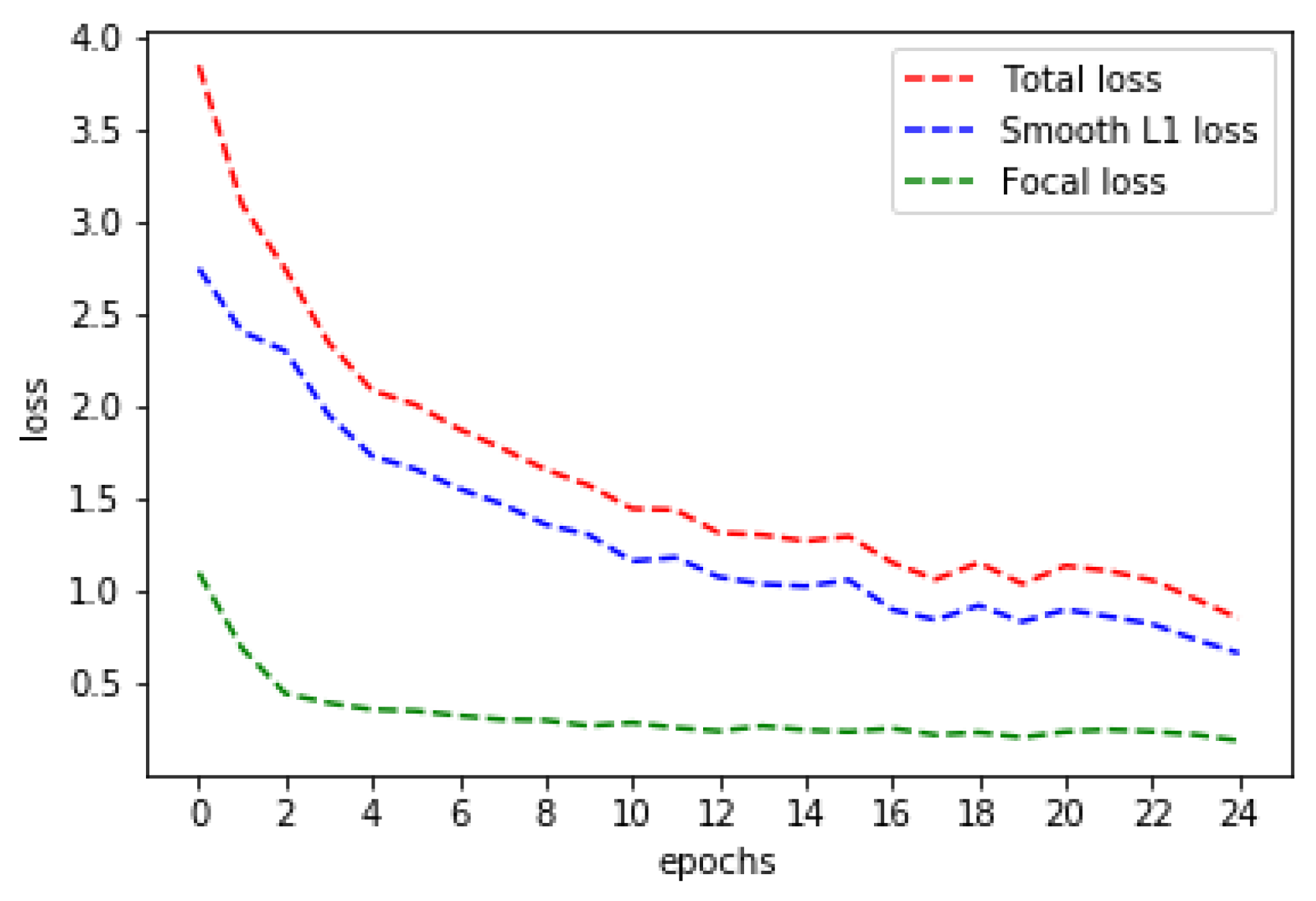
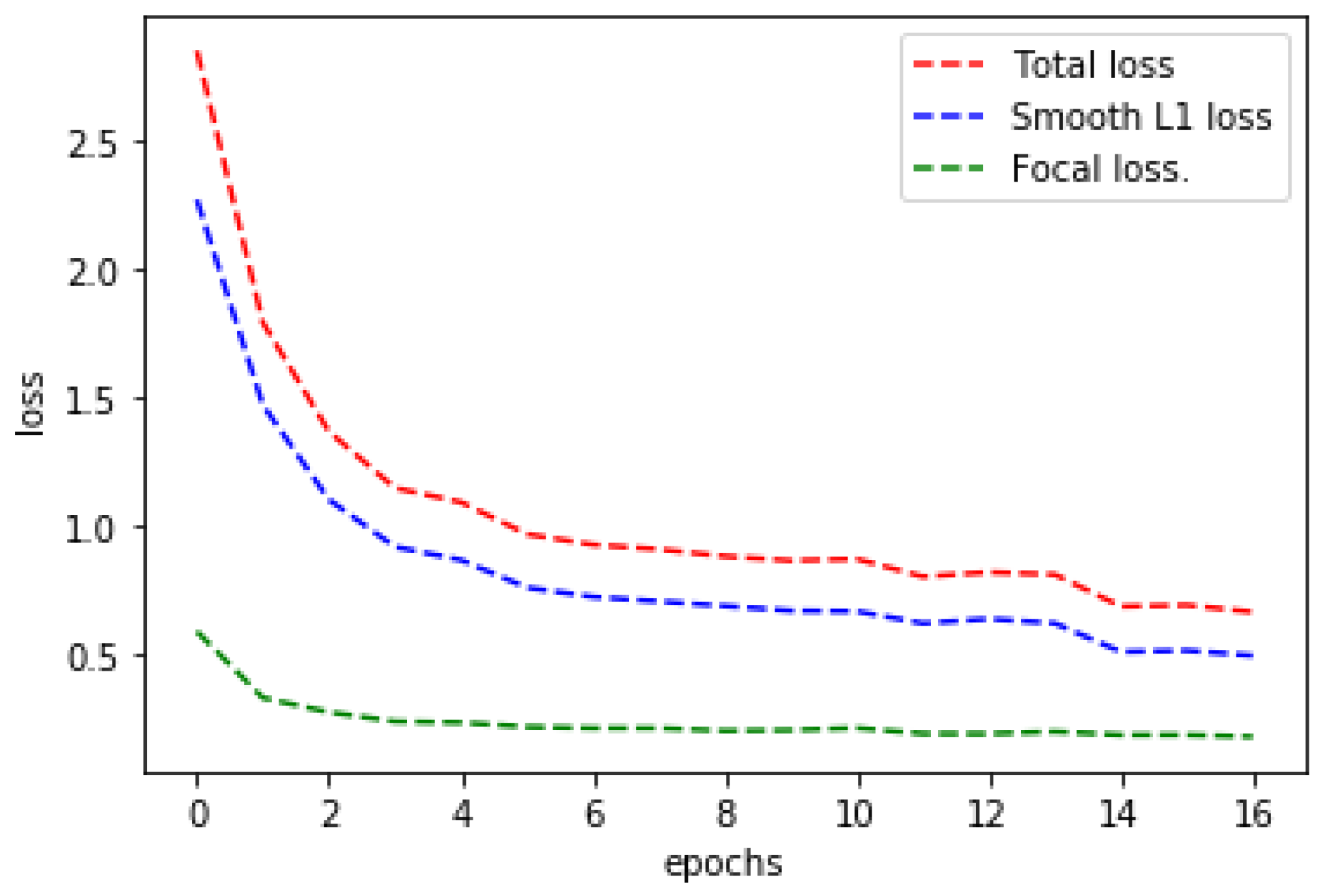
During training with the postfiltered training samples, the classification loss reached the minimum value of 0.17 after the 16th epoch, with a regression loss of 0.49 and a total loss of 0.66 (Figure 5). The calculated AP was 91.76 after training in epoch 16 (Figure 6). Training was stopped because no progress was made after five epochs, as measured by the AP.

The different test applications and the resulting metric are summarized in

Table 3. The table represents the TP, FP, FN, and TN as well as the precision and the recall for both test datasets.

	Random Images	Images with PV	Overall
TP	72	249	321
FP	8	17	25
FN	10	49	59
TN	2780	6160	8940
Precision	90.00	93.61	92.77
Recall	87.80	83.56	84.47

.

From the validation with randomly selected images, 72 correctly detected plants resulted, 8 objects were incorrectly detected as PV systems, and 10 PV systems could not be detected. A total of 2780 buildings without PV systems were correctly assigned to the background class. This resulted in a precision of 90.00 and a recall of 87.80. In the dataset additionally enriched with PV systems, 249 correctly detected PV systems, 17 objects incorrectly detected as PV systems, and 49 nondetected PV systems result. A total of 6160 buildings were included in the background class. The precision achieved was 93.60 and the recall was 83.56. The overall metrics summing up both test applications resulted in a precision of 92.77 and a recall of 84.47. 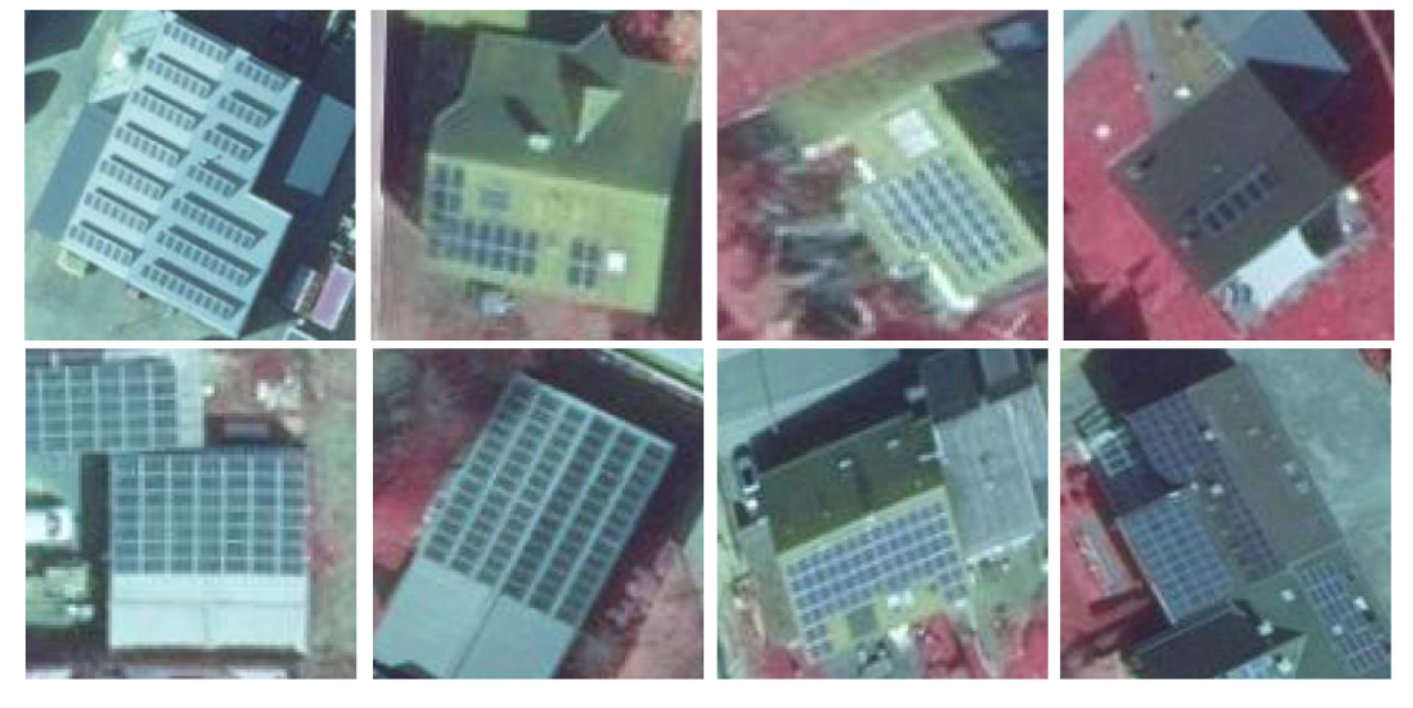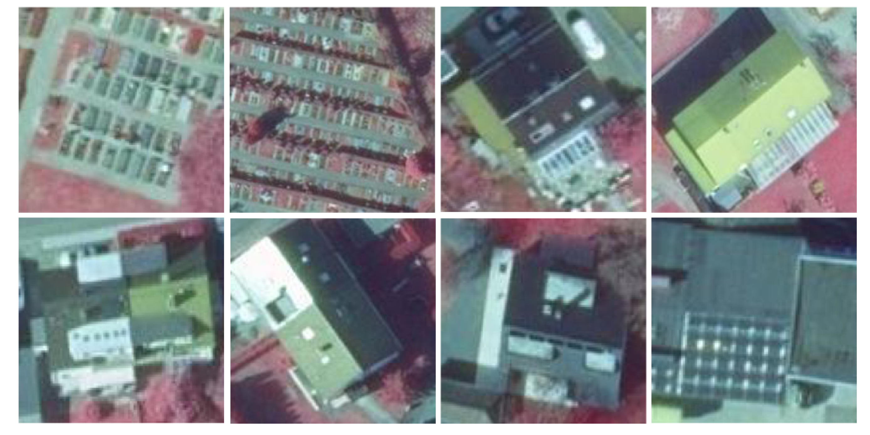Figure 7 shows a selection of correctly detected objects.

Figure 8 shows a selection of false positives. The objects in the first two pictures are not buildings. Furthermore, wrongly classified objects include canopies, patio roofs, and conservatories, as shown in the third and fourth picture. The second row shows objects where it is not possible to see whether they are PV systems or not.

5. Discussion

Using the two cases of the test application, the accuracy of the model was tested by selecting randomly drawn images, and in a dataset enriched with PV systems. It can be clearly observed that the enrichment of TP examples leads to a higher precision, whereby the recall decreases. Looking at the FP examples, repetitive patterns become visible. Particularly canopies, patio roofs, and conservatories are detected. The examples classified as FPs, which are not buildings, could be filtered in a real application based on the overlaps of the HU-DE, which could increase the quality of the application.

The FP examples that cannot be clearly assigned can be used as good examples of the challenge of remote-supported procedures in dealing with the creation of training areas. In some cases, the mere evaluation of the available image data is not sufficient for correct classification. The large number of TNs compared to the TPs shows the enormously unevenly distributed class ratio, as the number of TNs represents all buildings without PV systems contained in the test images. Since the TN value is not included in the calculation of precision and recall, the number of TN does not affect the metric calculation.

The automated generation of large amounts of training data can, of course, also lead to some of the training samples being incorrect. A comparison of the first and second training shows that despite halving the number of samples from the first to the second training, better results were achieved. Thus, all loss values decreased further, the AP increased from 87.95 to 91.76. This effect is probably due to the reduction of incorrectly generated samples, which results in faster and better generalization during training.

Based on the proof-of-concept application, it can be shown that the developed workflow provides good results, with the semi-automatic processing of the training samples having the advantage of saving time by avoiding the time-consuming manual preparation of a large number of samples.

6. Conclusions

We developed a method for automated detection of buildings with PV systems. The generation of training data without manual selection allows the use of a large amount of training data. However, these may be inaccurate or erroneous. Comparisons of different tests suggested that postfiltering of the training data reduced the number of erroneous locations in a fully automated way. Based on the test application, the precision of the object detector was up to 92.77 and the recall was 84.47.

In future work, we will extend the procedure of semi-automated generation of object classes. By transferring the methodology to other classes of existing renewable energy plants such as wind turbines and biogas plants, the application can be expanded.

References

- Malof, J.M.; Hou, R.; Collins, L.M.; Bradbury, K.; Newell, R. Automatic solar photovoltaic panel detection in satellite imagery. In Proceedings of the 2015 International Conference on Renewable Energy Research and Applications (ICRERA), Palermo, Italy, 22–25 November 2015; pp. 1428–1431. [Google Scholar] [CrossRef]
- Malof, J.M.; Collins, L.M.; Bradbury, K.; Newell, R.G. A deep convolutional neural network and a random forest classifier for solar photovoltaic array detection in aerial imagery. In Proceedings of the 2016 IEEE International Conference on Renewable Energy Research and Applications (ICRERA), Birmingham, UK, 20–23 November 2016; pp. 650–654. [Google Scholar] [CrossRef]
- Malof, J.M.; Collins, L.M.; Bradbury, K. A deep convolutional neural network, with pre-training, for solar photovoltaic array detection in aerial imagery. In Proceedings of the 2017 IEEE International Geoscience and Remote Sensing Symposium (IGARSS), Fort Worth, TX, USA, 23–28 July 2017; pp. 874–877. [Google Scholar] [CrossRef]
- Yuan, J.; Yang, H.L.; Omitaomu, O.A.; Bhaduri, B.L. Large-scale solar panel mapping from aerial images using deep convolutional networks. In Proceedings of the 2016 IEEE International Conference on Big Data (Big Data), Washington, DC, USA, 5–8 December 2016; pp. 2703–2708. [Google Scholar] [CrossRef]
- Yu, J.; Wang, Z.; Majumdar, A.; Rajagopal, R. DeepSolar: A Machine Learning Framework to Efficiently Construct a Solar Deployment Database in the United States. Joule 2018, 2, 2605–2617. [Google Scholar] [CrossRef] [Green Version]
- Mayer, K.; Wang, Z.; Arlt, M.-L.; Neumann, D.; Rajagopal, R. DeepSolar for Germany: A deep learning framework for PV system mapping from aerial imagery. In Proceedings of the 2020 International Conference on Smart Energy Systems and Technologies (SEST), Istanbul, Turkey, 7–9 September 2020; pp. 1–6. [Google Scholar] [CrossRef]
- Zech, M.; Ranalli, J. Predicting PV Areas in Aerial Images with Deep Learning. In Proceedings of the 2020 47th IEEE Photovoltaic Specialists Conference (PVSC), Calgary, AB, Canada, 15 June–21 August 2020; pp. 0767–0774. [Google Scholar] [CrossRef]
- Tuia, D.; Volpi, M.; Copa, L.; Kanevski, M.; Munoz-Mari, J. A Survey of Active Learning Algorithms for Supervised Remote Sensing Image Classification. IEEE J. Sel. Top. Signal Process. 2011, 5, 606–617. [Google Scholar] [CrossRef]
- Liu, L.; Ouyang, W.; Wang, X.; Fieguth, P.; Chen, J.; Liu, X.; Pietikäinen, M. Deep Learning for Generic Object Detection: A Survey. Int. J. Comput. Vis. 2020, 128, 261–318. [Google Scholar] [CrossRef] [Green Version]
- Huang, X.; Weng, C.; Lu, Q.; Feng, T.; Zhang, L. Automatic Labelling and Selection of Training Samples for High-Resolution Remote Sensing Image Classification over Urban Areas. Remote Sens. 2015, 7, 16024–16044. [Google Scholar] [CrossRef] [Green Version]
- GeoBasis-DE/BKG, Deutsche Post Direkt GmbH, Statistisches Bundesamt, Wiesbaden. Georeferenzierte Adressdaten—GA. 2020. Available online: https://gdz.bkg.bund.de/index.php/default/georeferenzierte-adressdaten-ga.html (accessed on 24 November 2021).
- GeoBasis-DE / BKG. Hausumringe Deutschland: HU-DE. 2020. Available online: https://gdz.bkg.bund.de/index.php/default/amtliche-hausumringe-deutschland-hu-de.html (accessed on 24 November 2021).
- GeoBasis-DE / BKG. Digitale Orthophotos Bodenauflösung 20 cm (DOP20). 2019. Available online: https://gdz.bkg.bund.de/index.php/default/digitale-orthophotos-bodenauflosung-20-cm-dop20.html (accessed on 24 November 2021).
- Levenshtein, V. Binary Codes Capable of Correcting Deletions, Insertions and Reversals. Sov. Phys. Dokl. 1966, 10, 707. [Google Scholar]
- Singla, N.; Garg, D. String matching algorithms and their applicability in various applications. Int. J. Soft Comput. Eng. 2012, 1, 218–222. [Google Scholar]
- Lhoussain, A.; Hicham, G.; Abdellah, Y. Adaptating the levenshtein distance to contextual spelling correction. Int. J. Comput. Sci. Appl. 2015, 12, 127–133. [Google Scholar]
- Lin, T.Y.; Goyal, P.; Girshick, R.; He, K.; Dollar, P. Focal Loss for Dense Object Detection. In Proceedings of the 2017 IEEE International Conference on Computer Vision (ICCV), Venice, Italy, 22–29 October 2017; pp. 2999–3007. [Google Scholar] [CrossRef] [Green Version]
- He, K.; Zhang, X.; Ren, S.; Sun, J. Deep Residual Learning for Image Recognition. In Proceedings of the 2016 IEEE Conference on Computer Vision and Pattern Recognition (CVPR), Las Vegas, NV, USA, 27–30 June 2016; pp. 770–778. [Google Scholar] [CrossRef] [Green Version]
- Lin, T.Y.; Dollar, P.; Girshick, R.; He, K.; Hariharan, B.; Belongie, S. Feature Pyramid Networks for Object Detection. In Proceedings of the 2017 IEEE Conference on Computer Vision and Pattern Recognition (CVPR), Honolulu, HI, USA, 21–26 July 2017; pp. 936–944. [Google Scholar] [CrossRef] [Green Version]
- Girshick, R. Fast R-CNN. In Proceedings of the 2015 IEEE International Conference on Computer Vision (ICCV), Santiago, Chile, 7–13 December 2015; pp. 1440–1448. [Google Scholar] [CrossRef]
- Gaiser, H.; de Vries, M.; Lacatusu, V.; Williamson, A.; Liscio, E.; Henon, Y.; Gratie, C.; Morariu, M.; Ye, C.; Zlocha, M.; et al. Fizyr/Keras-Retinanet 0.5.1. 20 June 2019. [Google Scholar] [CrossRef]
- Wolf, S.; Sommer, L.; Schumann, A. FastAER Det: Fast Aerial Embedded Real-Time Detection. Remote Sens. 2021, 13, 3088. [Google Scholar] [CrossRef]
- Xiao, Z.; Wang, K.; Wan, Q.; Tan, X.; Xu, C.; Xia, F. A2S-Det: Efficiency Anchor Matching in Aerial Image Oriented Object Detection. Remote Sens. 2021, 13, 73. [Google Scholar] [CrossRef]
- ZFTurbo. GitHub—ZFTurbo/Keras-RetinaNet-for-Open-Images-Challenge-2018: Code for 15th place in Kaggle Google AI Open Images—Object Detection Track. 2021. Available online: https://github.com/ZFTurbo/Keras-RetinaNet-for-Open-Images-Challenge-2018 (accessed on 24 November 2021).