Very High-Resolution Satellite-Derived Bathymetry and Habitat Mapping Using Pleiades-1 and ICESat-2

Abstract

Accurate and reliable bathymetric data are needed for a wide diversity of marine research and management applications. Satellite-derived bathymetry represents a time saving method to map large shallow waters of remote regions compared to the current costly in situ measurement techniques. This study aims to create very high-resolution (VHR) bathymetry and habitat mapping in Mayotte island waters (Indian Ocean) by fusing 0.5 m Pleiades-1 passive multispectral imagery and active ICESat-2 LiDAR bathymetry. ICESat-2 georeferenced photons were filtered to remove noise and corrected for water column refraction. The bathymetric point clouds were validated using the French naval hydrographic and oceanographic service Litto3D^® dataset and then used to calibrate the multispectral image to produce a digital depth model (DDM). The latter enabled the creation of a digital albedo model used to classify benthic habitats. ICESat-2 provided bathymetry down to 15 m depth with a vertical accuracy of bathymetry estimates reaching 0.89 m. The benthic habitats map produced using the maximum likelihood supervised classification provided an overall accuracy of 96.62%. This study successfully produced a VHR DDM solely from satellite data. Digital models of higher accuracy were further discussed in the light of the recent and near-future launch of higher spectral and spatial resolution satellites.

1. Introduction

Mapping coastal areas is essential to tackle a broad range of environmental and social issues [1,2,3]. Therefore, a wide variety of scientific research disciplines could benefit from a better knowledge of this interface, especially regarding the monitoring and protection of coral reefs in archipelagos or the production of navigational charts [4].

Numerous reliable and accurate techniques exist to acquire bathymetric soundings. Data are often obtained through marine surveys equipped with multibeam or single-beam echosounders [5]. However, these approaches are usually impracticable in remote and shallow areas as well as time consuming and limited in terms of spatial coverage, and therefore remain costly. As an alternative, remote sensing is increasingly used to retrieve coastal bathymetry. Airborne data acquired with bathymetric LiDAR are useful to map larger areas but remain costly and limited spatially [6,7].

Over the past few years, satellite-derived bathymetry (SDB) has been increasingly used as it offers a more affordable and time saving alternative. Scientific studies have demonstrated the possibility of obtaining reliable bathymetric data through hyperspectral and multispectral (MS) imagery at various spatial resolutions, due to a correlation between water depth and reflectance data [8,9,10,11]. Nevertheless, SDB mostly relies on passive imagery, which strongly constrains its use to clear and shallow water areas [12,13]. Depth can be retrieved from satellite MS imagery using physics-based or empirical models. Physics-based models rely on the physics or the radiative transfer of light in the water column and the physical properties of the water constituents that can be estimated with or without field measurements of depth for calibration. Some physics-based models are entirely based on the inversion of the radiative transfer model, such as WASI and BOMBER, but they can be complex to implement [14,15,16]. On the other hand, empirical models are limited by the need to calibrate the MS imagery with in situ measurements [17,18].

There is a real need for producing bathymetric data solely from satellite images. In this context, the launch of the NASA Ice, Cloud, and Land Elevation Satellite-2 (ICESat-2) in September 2018 offered new prospects [19]. This satellite aims to monitor the cryosphere and terrestrial biosphere using the green 532 nm LiDAR with photon-counting capability. Pre-launch studies highlighted its potential to penetrate the upper part of the water column and reach the bottom [20]. A pioneer study has recently validated accurate ICESat-2 bathymetry retrieval at 38 m depth in very clear waters [21]. A second relevant study used ICESat-2 bathymetric measurements, down to 18 m depth, to calibrate and validate Sentinel-2 imagery at 10 m pixel size [17]. This spatial resolution nonetheless remains limiting for some applications (e.g., marine ecology, navigation).

Our paper aims to create a higher resolution digital depth model (DDM) by fusing active ICESat-2 bathymetric soundings and 0.5 m Pleiades-1 passive MS imagery in order to provide very high-resolution (VHR) satellite-based bathymetry and habitat maps of the coral reefscapes in Mayotte. First, a density-based algorithm was implemented on ICESAt-2 ATL03 L2 dataset to remove the noise in photon data and detect the water surface. The noise arises from several sources, including the laser pulse being scattered by the atmosphere, the solar background noise effects, and the detector dark noise. In our study, the main noise source is associated with photons that are scattered by particles in the water column [22]. Based on this first clustering, photons from the seabed were identified and corrected for the refraction effect occurring at the air-water interface. Producing bathymetric maps requires finding a function that describes the relationship between bathymetry measurements and the remotely sensed spectral values of the satellite image [8]. In this study, we used the band ratio model developed by [23]. First, we derived the above water surface reflectance log ratio of two spectral bands. Then, we characterized the relationship between the ratio and ICESat-2 water depth measurements [17]. Therefore, this study innovatively produces a VHR DDM and VHR benthic habitats map of the area from satellite data without a need for in situ measurements. Bathymetric data were used to remove the effect of the water column and generate a digital albedo model (DAM) to classify benthic habitats [24,25,26,27]. Finally, the vertical accuracy of the predicted depths was assessed by comparing the bathymetric data to the French naval hydrographic and oceanographic service SHOM bathymetric LiDAR and multibeam echosounder reference dataset (Litto3D^®). Classification performances were evaluated using a confusion matrix.

2. Materials and Methods

2.1. Study Site and Data

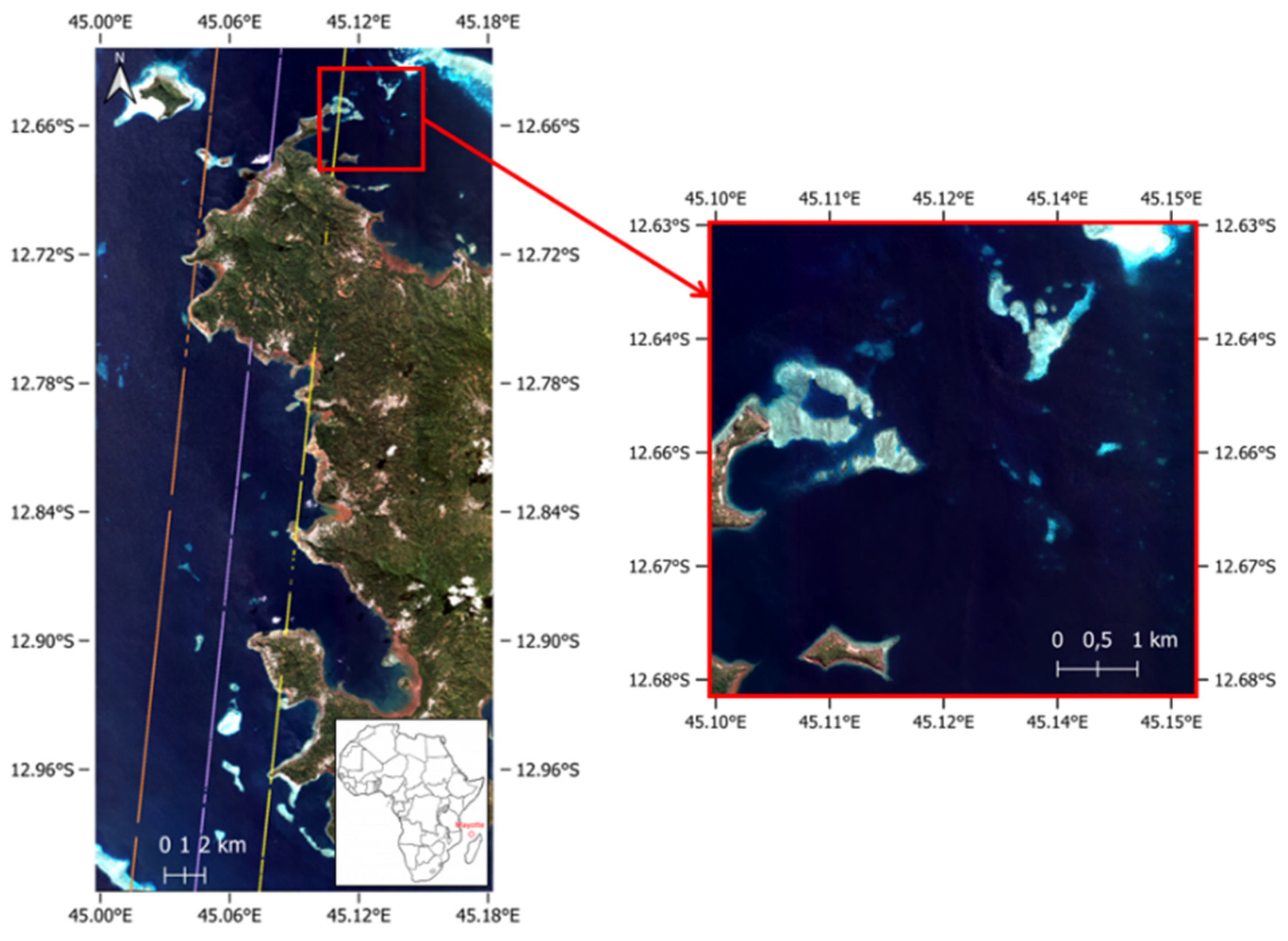
2.1.1. Study Site

The study site is located in the northwest of the island of Mayotte (latitude: 12.63°−12.68°S, longitude: 45.10°−45.15°E), a French overseas territory located in the southwest Indian Ocean (Figure 1). This site is partially sheltered from wind and wave influence, factors known to affect the quality of SDB estimates. Mayotte coasts offer a wide variety of marine fauna and flora strongly affected by global climate and local anthropogenic changes, requiring environmental monitoring [1,3]. This region was also selected due to the availability of high-resolution airborne bathymetric LiDAR and multibeam echosounder data necessary for validation.

Water clarity is a key parameter in SDB estimation. Clarity is related to light ray penetration in the water column, thus impacting the quality and quantity of the available bathymetric soundings [27,28,29,30,31]. This variable can be estimated using a diffuse attenuation coefficient of 490 nm measured at 4 km resolution by the moderate-resolution imaging spectroradiometer (MODIS-Aqua, publicly accessible from https://oceancolor.gsfc.nasa.gov/l3/, last accessed: 28 December 2021) [32]. A diffuse attenuation coefficient value of 0.0615 m⁻¹ was obtained for the month of May 2020 for the study site, indicating a very clear water type. Previous studies using ICESat-2 for bathymetric estimations had a diffuse attenuation coefficient ranging from 0.032 m⁻¹ for the Virgin Island to 0.123 m⁻¹ for the Bahamas, both known to be areas with very clear water [21,33].

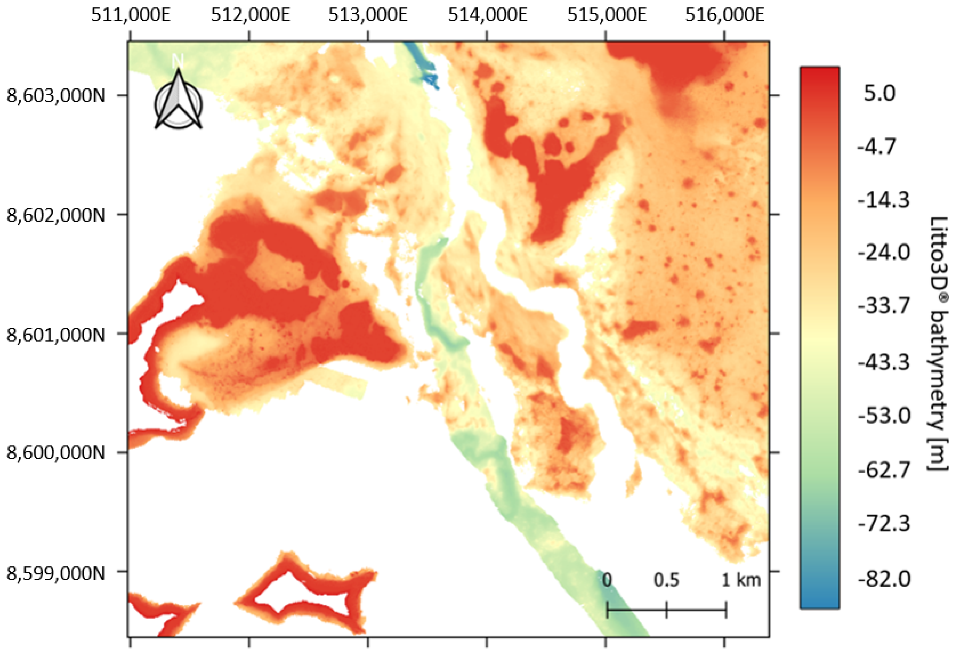
2.1.2. Litto3D^® Reference Dataset

The French Oceanographic and Hydrographic Marine Service (SHOM) and the French National Institute for Geographical and Forest Information (IGN) conducted a joint altimetric and hydrographic survey of Mayotte from 2003 to 2010. Most of the island was mapped using the airborne topographic and bathymetric LiDAR and multibeam echosounder. The resulting Litto3D^® product provides soundings located in a three-dimensional geometric reference system with high spatial resolution and a land-sea continuum (data are available for free from https://diffusion.shom.fr/, last accessed: 28 December 2021). Data extracted from this dataset, corresponding to the ICESat-2 ground track, and used for comparison, include bathymetric points acquired using the bathymetric LiDAR and multibeam echosounder.

Litto3D^® soundings are provided in a cartesian coordinate system in the horizontal plane and with orthometric heights. The point cloud density is constrained by the acquisition method over a specific area and the gridded model is provided with a spatial spacing of either 1 m or 5 m. Specification regarding the positioning and the geodesy of the Litto3D^® dataset are presented in

Table 1. Specifications of the Litto3D^® dataset acquired over Mayotte.

Geodetic system	RGM04
Ellipsoid	IAG GRS80
Projection	UTM 38 S
Vertical frame	Orthometric heights (MAYO53)

[34]. A local geoid, RGM04, was used as a reference for this dataset.

This dataset was used during the validation phase to measure the accuracy of the SDB, but Litto3D^® data were not used as calibration points for the models.

2.1.3. Pleiades-1A Multispectral Satellite Imagery

A MS Pleiades-1A imagery acquired on 25 May 2020, at 07 h 24 min UTC, was provided by the French space agency CNES through the data platform DINAMIS (https://dinamis.data-terra.org/, last accessed: 28 December 2021). Pleiades-1A imagery is delivered with four MS bands at 2 m pixel size, with an 11-bit dynamic range: Blue (430–550 nm), green (500–620 nm), red (590–710 nm), and near infrared (740–940 nm). Moreover, a panchromatic band at 0.5 m pixel size (470–830 nm) is included, with the same radiometric resolution [35]. The four-band imagery is geometrically projected with the WGS84/UTM38S coordinate system and radiometrically corrected to units of top of atmosphere (TOA) reflectance.

2.1.4. ICESat-2 LiDAR Satellite Soundings

ICESat-2 is in a near-polar orbit at an altitude of 496 km and operates with a revisit period of 91 days over oceans [19,36]. ICESat-2 was mainly designed to measure icesheet topography, sea ice, and various inherent properties of the atmosphere and terrestrial vegetation, although ocean and inland surface waters are also observed. The Advanced Topographic Laser Altimeter (ATLAS), a photon-counting LiDAR, is the only sensor onboard the satellite, emitting a green laser beam at a wavelength of 532 nm. ATLAS enhances spatial sampling by splitting the laser beam into three pairs of beams separated by 3.3 km. Each pair, separated by 90 m, consists of a “weak” energy beam and a “strong” beam with a four-fold higher pulse energy [19,36]. ICESat-2 data can be downloaded with different degrees of processing, depending on the users’ needs. This study uses the 3rd version of the L2 ATL03 georeferenced photons (data publicly available at https://search.earthdata.nasa.gov/search, last accessed: 28 December 2021) [37]. Data about each photon are provided with the latitude, the longitude, and the height relative to the WGS84 ellipsoid as well as other ancillary information. Considering that ICESat-2 was not designed to study the sub-surface water or the bottom topography, it is necessary to include in the analyses a correction for refraction bias induced by the water column.

We selected the ICESat-2 track acquired on the date closest to the acquisition date of the MS imagery. The two datasets were acquired 10 days, 10 h and 33 min apart. Then, the specific study area in Mayotte was selected based on the range of depths for which calibration data were available. ICESat-2 passed over Mayotte on 14 May 2020, at 20 h 51 min UTC, and collected bathymetric data down to a depth of 15 m.

2.2. Data Processing

Most of the ICESat-2 photons that reach the oceans penetrate into the water. However, compared to the water surface returns, only a small fraction is returned from the water column backscatter and bottom reflectance. Therefore, ICESat-2 signal photons correspond primarily to the water surface reflectance, water column backscatter, seabed reflectance, and noise.

ICESat-2 ATL03 data are provided with a preliminary classification of every photon regarding how likely it is to be signal or noise (confidence levels are: Noise, Low, Medium, High, and Buffer). Photons classified as “Buffer” are identified after all the signal photons are clustered. These are the photons for which doubt remains, which are at the limit to be identified as part of the signal. Therefore, this category has been created to ensure that all of the photons identified as signal are present in the corrected product [37]. Figure 2 presents the transect used in this study, indicating the original classification of the georeferenced photons. In this figure, photon positions (latitude and longitude) were projected onto a local geographic plane. Therefore, the horizontal axis corresponds to the along track distance. The origin point corresponds to the northernmost location of the trajectory. However, this clustering is not suited to underwater environments as it considers a considerable amount of the seafloor as noise. Therefore, all of the photons were considered and a modified density-based spatial clustering of application with noise (DBSCAN) algorithm was used to separate the photons characterizing the noise and the sea surface from those related to the seabed [17,38,39,40].

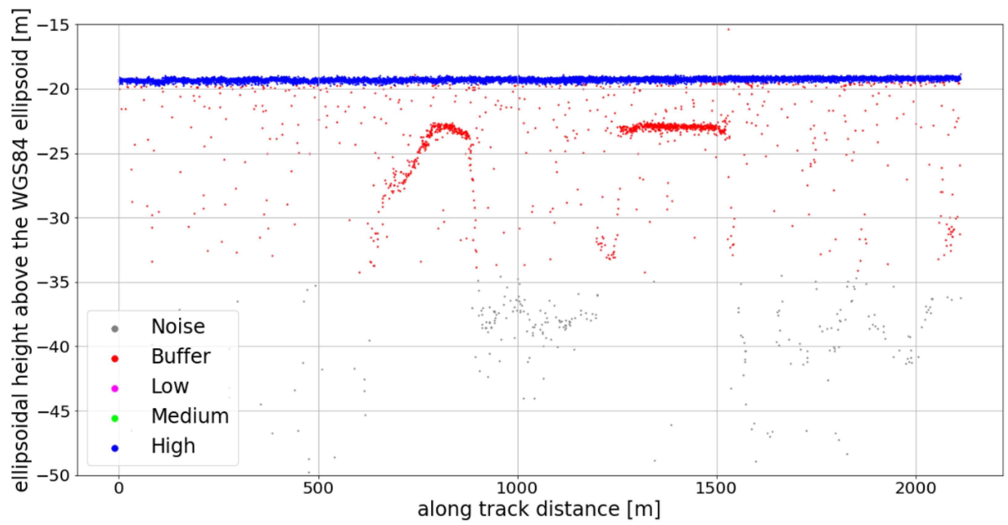
2.2.1. Noise Removal and Detection of the Sea Surface

In the dataset, noise corresponds to sparse points with a low spatial density compared to the sea surface and seabed clusters. Georeferenced photons likely to be noise were removed, and photons associated with the sea surface were identified.

Here, a density-based spatial clustering method was used, which is an unsupervised learning method used to identify clusters in a dataset. The method is based on the premise that each cluster is defined as a region of points with a given density and spatially isolated from other groups by areas of lower density. The DBSCAN algorithm used scanned the entire dataset and established a search radius on each point successively. The point considered during a given step is a “core point”. DBSCAN allows the users to specify a search radius size according to two criteria: The search circle radius ϵ and the minimum number of points MinPts. Once a criterion is no longer satisfied, the algorithm begins a new classification group [41].

Previous studies successfully implemented DBSCAN on the ICESat-2 dataset of islands located in the south of China and in the Bahamas. One particular study provides formulas to configure the MinPts and the ϵ radius parameters of the DBSCAN algorithm [17]. In the present research, the search radius was manually chosen by the user to guide the clustering process and optimize the results. In addition, the MinPts parameter is defined by Equation (1) [17] (this formula is suited for a study of a water column whose depth is not expected to exceed 60 m).

$$MinPts=\frac{2S{N}_1-S{N}_2}{\ln \left(\frac{2S{N}_1}{S{N}_2}\right)},$$

(1)

where SN₁ is the number of expected photons corresponding to signal and noise and defined by Equation (2):

$$S{N}_1=\frac{ \pi {ϵ}^2{N}_1}{hl},$$

(2)

where N₁ is the total number of photons (both signal and noise), h is the vertical range and l is the along track range. SN₂ is the expected noise photons number and is defined by Equation (3):

$$S{N}_2=\frac{ \pi {ϵ}^2{N}_2}{h_{2}l},$$

(3)

where N₂ corresponds to the number of photons in the layer with the fewer bathymetric photons, while h₂ is the height of the corresponding layer [17].

The variable MinPts is constrained to a value no lower than 3. If the previous formula provides a value lower than this threshold, then MinPts was set to 3 [17]. This algorithm might not be optimal in the present situation, since the dataset contains isolated photons from the seabed which could be identified as noise. Considering the small number of photons from the seabed, it was decided not to optimize the noise cleaning process, even if it meant that some manual cleaning had to be done. Therefore, the remaining noise points were removed manually using GlobalMapper software 22.1.0 (Blue Marble Geographics, Hallowell, ME, USA).

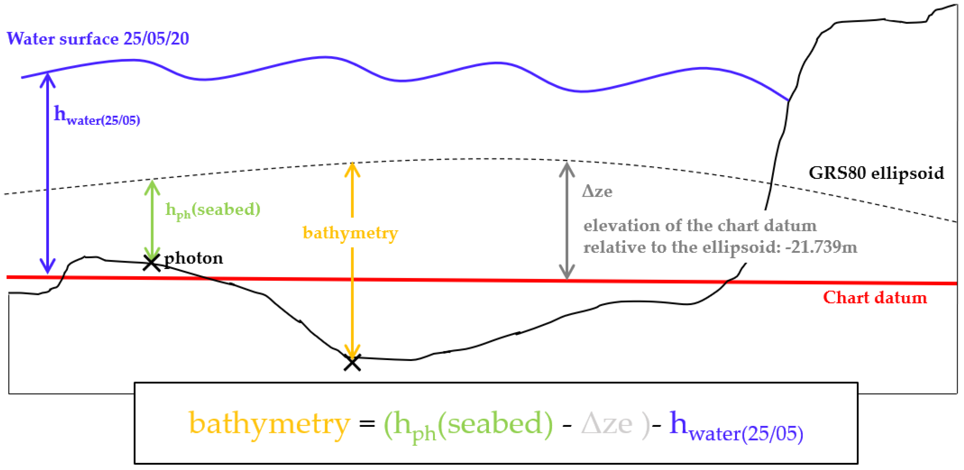
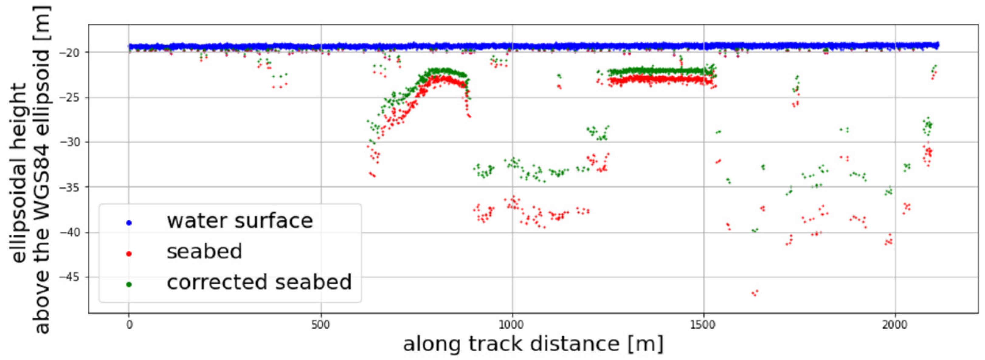
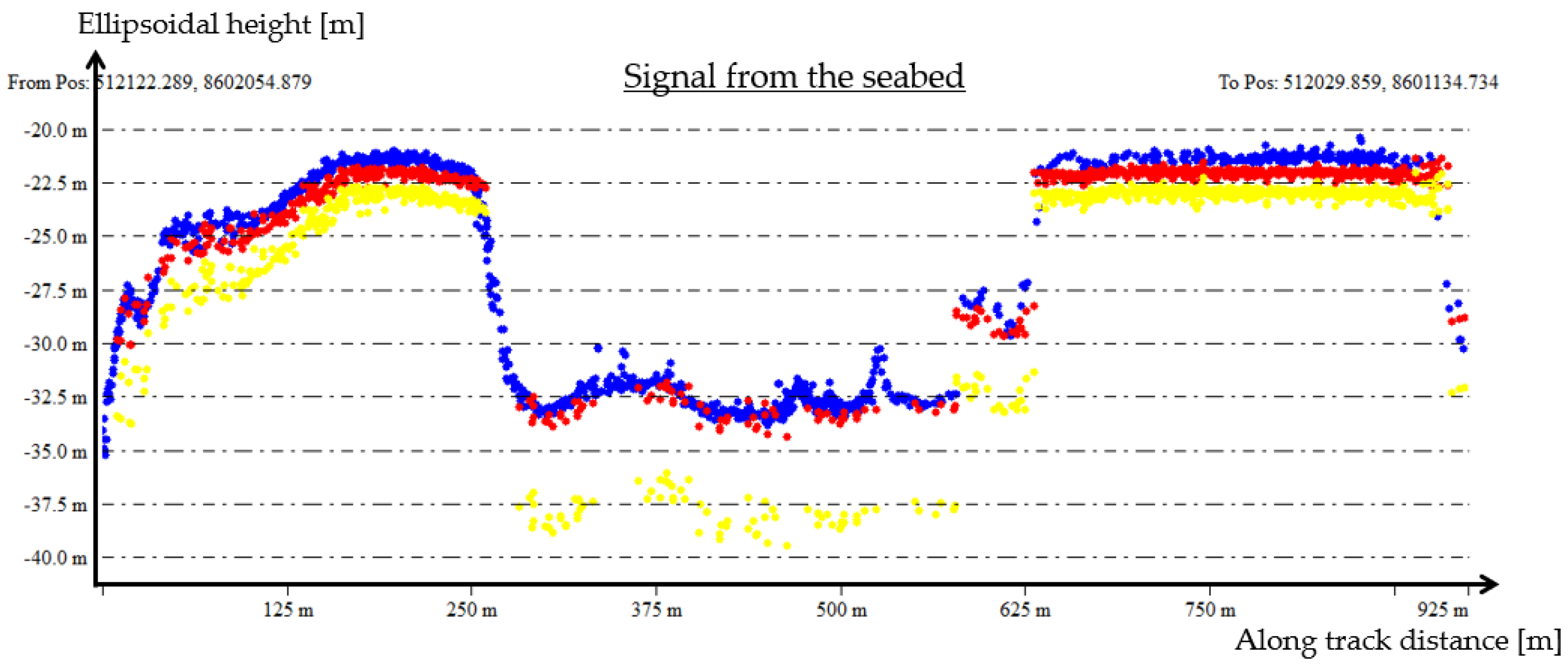
2.2.2. Detection of the Seabed

The sea surface is the cluster with the highest number of photons. It is a high-density group of photons spread over a continuous line, depending on the state of the sea. The sea surface cluster is clearly visible in blue in Figure 2.

According to [17], after removing the noise, the seabed is defined as every signal photon below a threshold value underneath the water surface. Therefore, every photon whose elevation is lower than LMS-3SV (where LMS is the Local Mean Sea level and SV the Surface Variance), was identified as a return signal from the seabed [17].

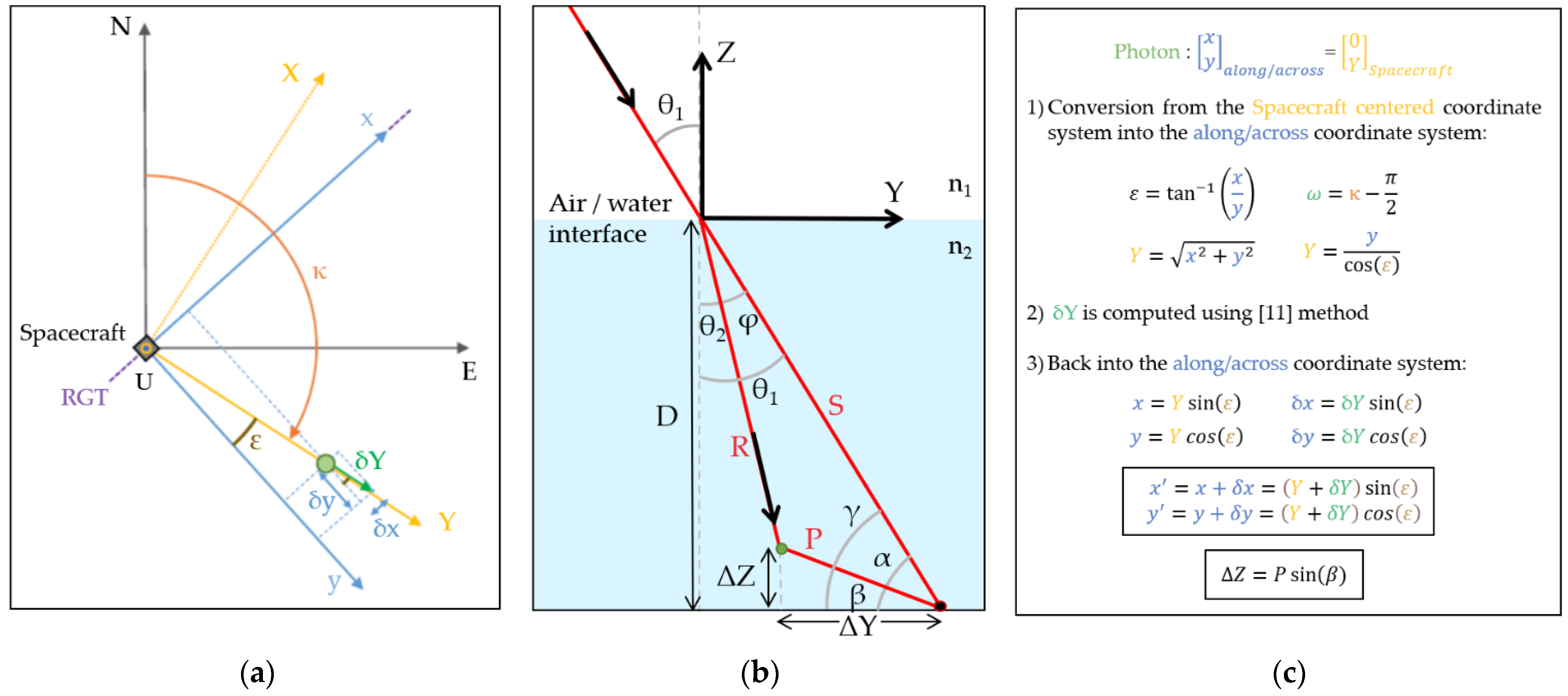
2.2.3. Correction for the Refraction Bias

Geolocated signal photons located below the water surface are not corrected for the refraction effect that redirects the light, and thus the LiDAR beams. It induces a positioning bias for photons in the water layer that would impact the bathymetry estimate.

A relevant coordinate system is important to compute simple correction formulas. In this paper, the results presented were obtained using the coordinate system defined by [21] and the correction formulas were recomputed from this point. Corrections were applied in a satellite-centered coordinate system, where Z is the vertical direction (opposite to the direction of local gravity), and Y is orthogonal to Z (in the horizontal plane) and oriented along the azimuth of the pointing vector [21]. The resulting geometry is presented in Figure 3.

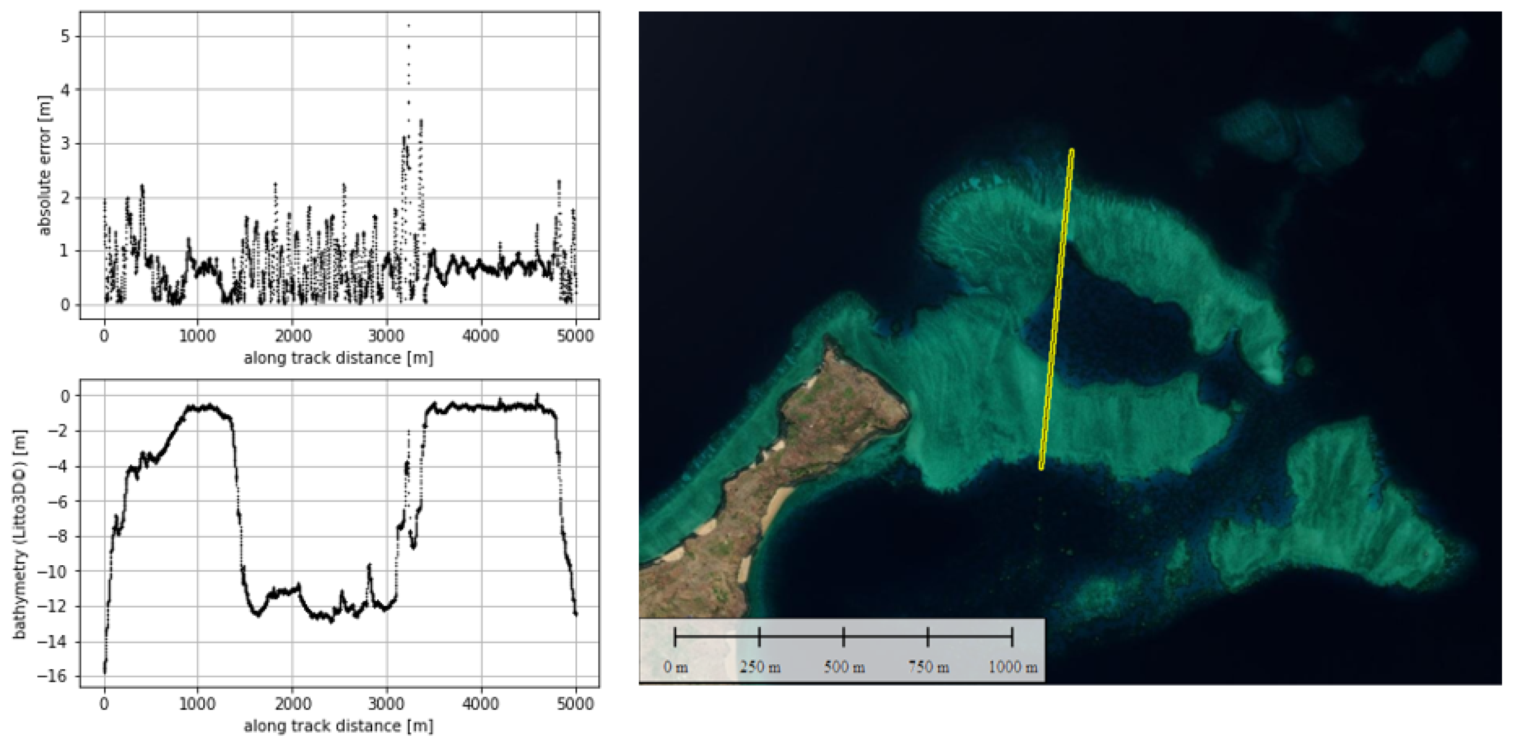
2.2.4. Validation of ICESat-2 Seabed Ellipsoidal Heights

The Litto3D^® dataset was used to validate the seabed photon ellipsoidal heights corrected from the refraction bias. While the ICESat-2 photons’ geographic coordinates are projected onto a local tangent plane (ENU) during the refraction bias correction, the vertical references are different. Soundings measured by the SHOM bathymetric LiDAR are provided with orthometric heights. The latter were converted into ellipsoidal heights (relative to the IAG GRS 80 ellipsoid) using Circe 5.2.1 (IGN free software). Data visualization and extraction were conducted in GlobalMapper software, and the points were processed using Spyder 4.15 python interpreter (an open-source MIT environment) to qualify the accuracy. The point density from Litto3D^® is considerably higher compared to the ICESat-2 dataset, it was interpolated to allow a comparison with the ICESat-2 dataset.

2.3. Satellite-Derived Bathymetry

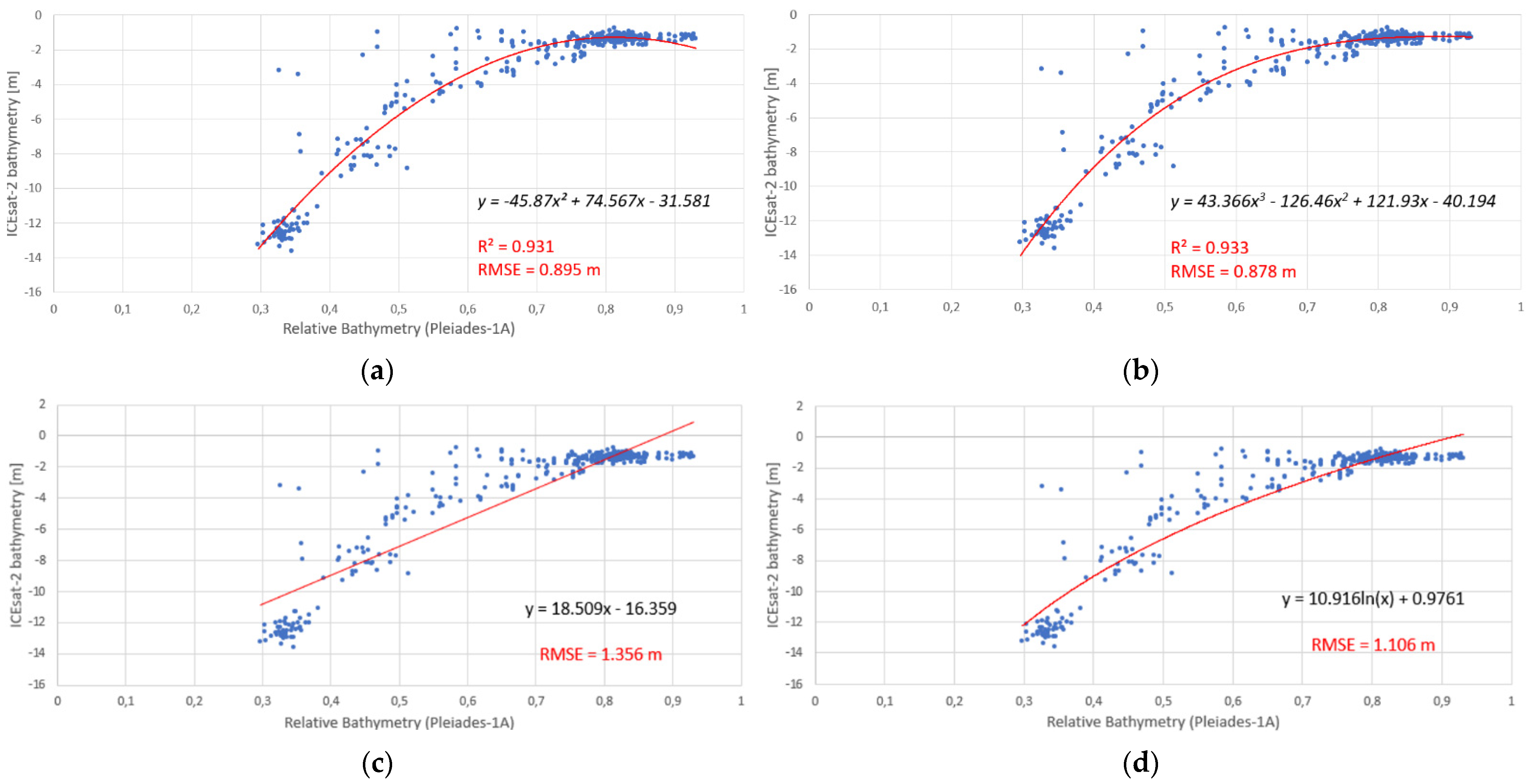
2.3.1. Ratio Transform Method

The SDB ratio transform algorithm provided by ENVI 5.3 (L3Harris Geospatial Solutions, Broomfield, CO, USA) was used to retrieve the relative DDM of the study area. The DDM is based on the relationship between reflectance and bathymetry, which is described by [23]. The semi-empirical model provides values of relative bathymetry by computing the logarithmic ratio of the reflectance of two spectral bands from a MS imagery. First, the 2 m pixel size imagery was converted into TOA reflectance values and was geometrically projected to the WGS84/UTM38S. At this point, the spatial resolution was enhanced using the Gram-Schmidt pan-sharpening method [42,43]. Second, the MS image was cropped with a spatial subset tool to isolate the geographical area of interest. Finally, the ratio transform was implemented with the algorithm developed by [23]. A map of the relative water depth (i.e., log ratio of the spectral bands) was derived from the log ratio between the green and blue spectral bands [44,45,46,47,48,49].

This method is one of the most commonly used methods in SDB studies, as it proved to provide accurate results and does not require many points for the calibration phase [18,23]. The advantages are that only two parameters need to be set and it works on all types of albedos. This method is also mainly suited for clear case 1 water, which is the case in this study [18,23].

Working with spectral band ratios is a way to compensate for the variability of ocean bottom type, since changes in the albedo values will affect approximately equally both spectral bands. On the contrary, a variation of depth has a higher impact on the spectral band, which is the most intensely absorbed in the water column. Therefore, depth is expected to be retrieved by this method independently of bottom albedo and can be obtained by inverting the radiative transfer equation as follows [23]:

$$z=m_1\frac{\ln \left(n{R}_w\left({\lambda }_j\right)\right)}{\ln \left(n{R}_w\left({\lambda }_i\right)\right)}-m_0,$$

(4)

where z is the depth, n is a constant needed for the ratio to stay positive, R_w is the reflectance of the water, m₀ is the offset for a depth of 0 m, and m₁ is the gain coefficient.

Each pixel of the MS imagery was assigned a value between 0 and 1. The final DDM was obtained by calibrating the relative bathymetry product with field-based depth measurements.

The final DDM was produced by finding the equation that best fits (i.e., lowest RMSE and higher R² with a simple equation formula) the relationship between the relative bathymetric values and the ground truth depth measurements. If bathymetric soundings measured by ICESat-2 are reliable and accurate enough, they could be used as a calibration/validation dataset to produce bathymetry solely from satellite observations.

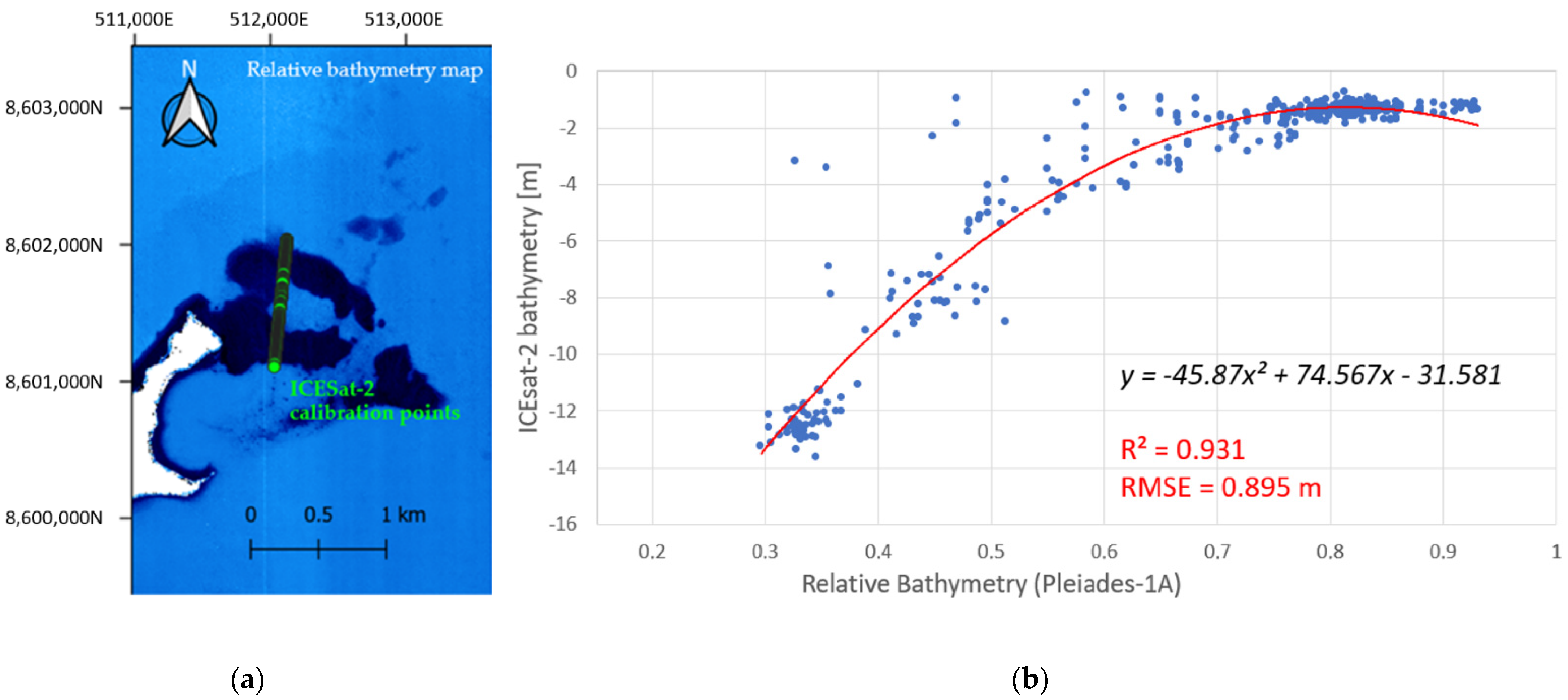
2.3.2. Calibration with ICESat-2 Soundings

During the calibration phase, pixels from the relative DDM were matched to bathymetric points measured by ICESat-2.

To produce a DDM, i.e., a map of the water height at the acquisition date of the satellite MS imagery, ICESat-2 vertical heights were converted into the appropriate datum. First, the ellipsoidal heights measured by the ICESat-2 satellite were referenced to the IAG GRS 80 ellipsoid and had to be referenced to the chart datum. The SHOM (https://data.shom.fr/, last accessed: 28 December 2021) provides accurate altimetric information over Mayotte island, including the distance between the ellipsoid and the chart datum in Dzaoudzi locality (distance of −21.74 m). Second, the water height above the chart datum, at the acquisition time of the MS satellite imagery, was added. The closest tide gauge from the study site was also located at Dzaoudzi and the measurements were available from the SHOM website. The tide gauge recorded a water height of 1.02 m above the chart datum on 25 May 2020, at 07 h 24 min UTC. Figure 4 illustrates the different variables involved to compute the bathymetry from ICESat-2 ellipsoidal heights.

Relative bathymetry points from the MS imagery were collected at the exact same location as the measurement points of ICESat-2 and an equation linking the two datasets was determined. Finally, the equation was applied to the relative DDM using the ENVI band math tool to generate the final DDM.

2.3.3. Digital Depth Model Validation

We compared different regression models. The aim was to find the model that best matches the bathymetry measurements of ICESat-2 with the remotely sensed spectral values of Pleiades-1A. The best regression was chosen based on the RMSE and based on the coefficient of determination, R². The final DDM was validated in comparison to the Litto3D^® reference dataset by computing the root mean square error (RMSE) and the maximum absolute error (MAE) statistical indicators.

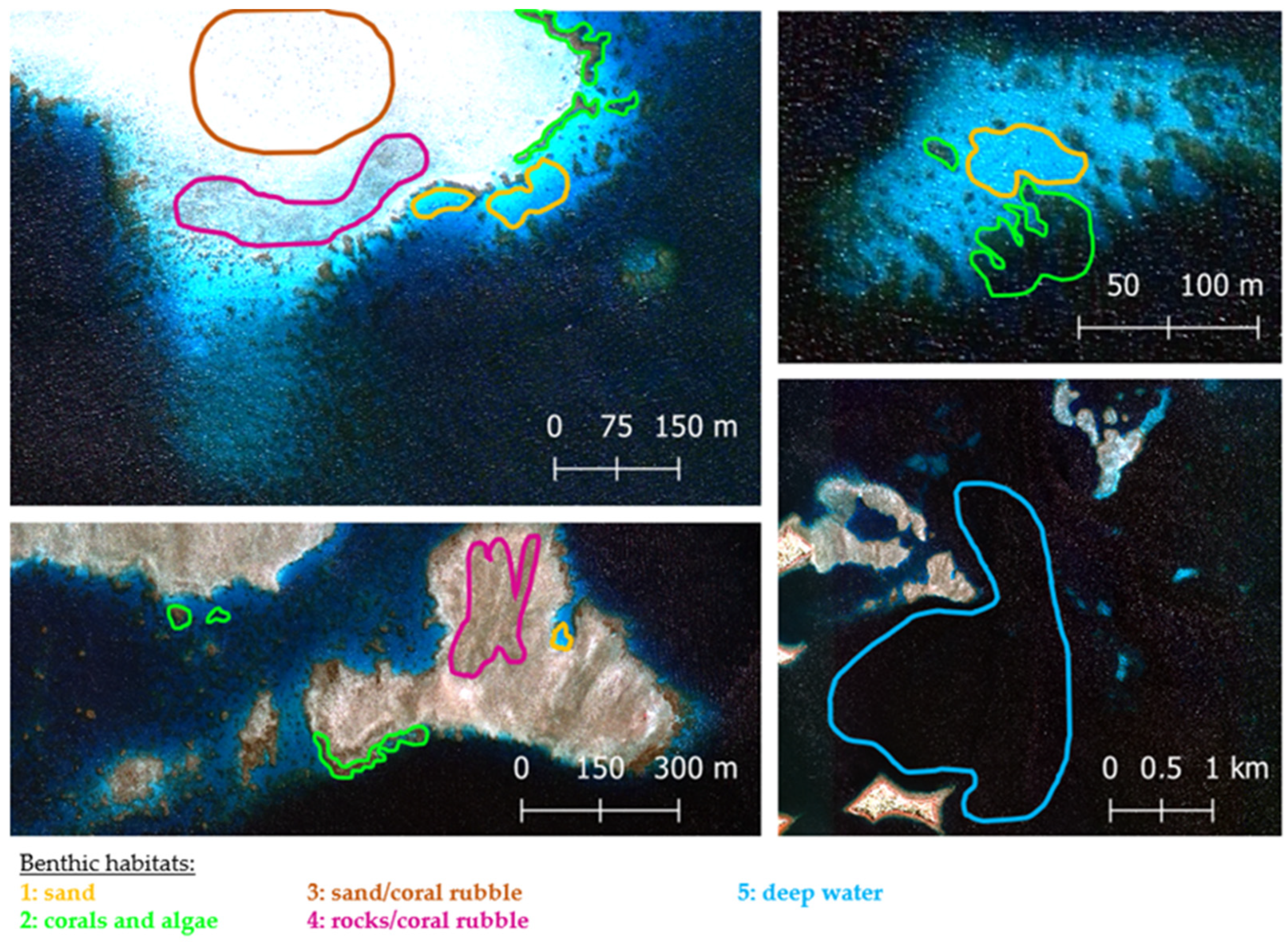
2.4. Benthic Habitats Mapping

2.4.1. Processing of the Multispectral Imagery

This paper further intends to classify the seabed into five general types: Sand, sand with coral rubble, rock with coral rubble, corals and algae, and deep water. The classification is based upon a DAM obtained from the MS imagery and the DDM.

In theory, it would be feasible to train the classification algorithm directly on the MS imagery, without any preliminary corrections. It would also be conceivable to add a fifth spectral band, corresponding to the bathymetry, to add extra information for the algorithm to get better results. However, this method was not optimal as classifying MS imagery without correcting the image for the decay of light rays in the water column might induce confusion between the spectral signatures of benthic habitats [50]. A better solution was to generate a DAM. Bathymetric data are necessary to quantify the loss of light in the water column, to compensate for this loss, and finally to obtain a DAM [25,50]. Benthic albedo values were obtained with Equation (5) [25]:

$$A_b=\left(R_w-R_{\infty }\right)e^{2K_{d}z}+R_{\infty }$$

(5)

where A_b is the bottom albedo, R_w is the water column reflectance, R_∞ is the reflectance in deep water, and K_d is the diffuse attenuation coefficient.

The TOA reflectance value for each spectral band was obtained after processing. First, the 2 m pixel size MS imagery was cropped to the area of interest and then orthorectified. Second, the image was converted into bottom of atmosphere (BOA) reflectance values using the FLAASH algorithm (see [50] for further details). At this point, it was possible to enhance the spatial resolution using pan-sharpening. These reflectance values were applied in Equation (5) to remove the water column contribution and obtain a bottom of hydrosphere (BOH) reflectance imagery from the BOA reflectance imagery.

The diffuse attenuation coefficient K_d was estimated for every spectral band of the visible range using values from a previous study on case 1 waters [51]. Values were given for a wide range of wavelength and were weighed with the appropriate factor found according to the wavelength sensitivities of Pleiades-1A sensor. Finally, an average value of K_d was computed for the three spectral bands in the visible range (

Table 2. Diffuse attenuation coefficient (K_d) for every spectral band of Pleiades-1A sensor in the visible range.

Spectral Band	λ [nm]	Kd [m−1]
Blue	(430–550)	0.0211
Green	(500–620)	0.0659
Red	(590–710)	0.2635

).

2.4.2. Supervised Classification Process

Similar to most coastal areas worldwide, the study area is lacking high-resolution benthic habitat data. Therefore, the supervised classification process was based on a visual identification of marine habitats assisted by two local marine scientists familiar with the area. The visual mapping by these experts was performed using the 0.5 m MS BOH reflectance imagery and the 0.5 m MS TOA reflectance imagery in parallel. Five benthic habitats were identified on several areas of the MS imagery (see Figure 5).

Corals are often visible on the edges of patch reefs. They appear in the form of brown and dark slender spots on the MS imagery and they are often colonized by algae. Sand areas are very bright areas often found on the border of the patch reefs, alongside corals. Two other main categories of benthic habitats can be distinguished. The first one corresponds to a mix of sand and coral rubbles. It appears as bright areas with dark brown spots. The other group contains mainly rocks and coral rubbles and appears as dark areas. While coral colonies are found on the edges, these two areas are often located towards the inner parts of the patch reefs. Coral rubbles are often transported towards the inner part of patch reefs by waves. Finally, both deep water areas, where the bottom was not visible, and land areas were masked.

In an attempt to enhance the classification accuracy, the albedo imagery was separated according to depth ranges. A first mask was created to suppress the depth values higher than the highest depth value measured by ICESat-2 over the area (i.e., 15 m). Then, the extinction depth of every spectral band was computed based on [50,51] (see

Table 3. Extinction depths for every spectral band of Pleiades-1A in the visible range.

Spectral Band [nm]	Average for Kd [m−1]	Extinction Depth (1/Kd) [m]
Blue (430–550)	0.211	47.4
Green (500–620)	0.0659	15.2
Red (590–710)	0.263	3.8

for results).

A first DAM was created for depths in the range of 0–3.8 m using three spectral bands (Red, Green, and Blue). A second DAM was created for depths in the range of 3.8–15 m using two spectral bands (Green and Blue), as the extinction depth of the red band was exceeded. Due to the fact that some habitats are not present in the studied depth range, two sets of regions of interest (ROI) were created for each DAM. The DAM with the lower depth range was classified using four ROIs, namely: Sand, coral and algae, sand and coral rubble, and rocks and coral rubble. The DAM with the higher depth range was classified using three ROIs, namely: Sand, coral and algae, and deep water.

Moreover, a choice of three morphological predictors was made to complement the MS bands of the DAM in order to enhance the classification results. The first predictor added was the slope before adding the aspect and the profile convexity all together. Classifications were computed using a 3 × 3 pixel kernel size.

Three classification algorithms were compared in this study: Neural network (NN), maximum likelihood (ML), and support vector machine (SVM).

2.4.3. Validation of the Supervised Classification

A validation dataset based on the MS imagery was produced with the same knowledge as for the calibration phase. A post-classification accuracy assessment using a confusion matrix provided information on overall accuracy (OA) and the kappa coefficient (κ) [52,53].

The ML and the SVM classifiers were set with the default parameters. A neural network classification was implemented with one and three hidden neurons in one hidden layer, in order to test the depth of the neuronal architecture.

3. Results

3.1. DDM

3.1.1. Correction of ICESat-2 Dataset

The ICESat-2 gt1l transect from the 2020 dataset corresponds to the strong beam and presents some variability in the depth range. The results obtained in this study, after removing the noise photons and correcting the signal for refraction bias, are presented in Figure 6. For comparison, the official signal detection and classification provided with the downloaded L2 ATL03 dataset were presented in Figure 2.

In Figure 6, photon positions (latitude and longitude) were projected onto a local geographic plane. Therefore, the horizontal axis corresponds to the along track distance. The origin point corresponds to the northernmost location of the trajectory. For the current study, the analysis indicates that (1) points from the seabed detected in this study are following the bottom topography, distinguishable on the satellite imagery; (2) while the ATL03 data classified with a high and medium confidence level (corresponding to the blue and green points in Figure 2) are located at or close to the surface, our bathymetry algorithm correctly identifies the bottom topography from low and buffer confidence points, a much smaller portion of the returned signal; and finally (3) the ATL03 dataset removed only a small fraction of the noise photons in comparison to the results generated with the DBSCAN.

The DBSCAN algorithm was configured based on an empirical approach with the value ϵ = 0.65 m. This value, valid for our study area, allowed us to retrieve a majority of the seabed signal while eliminating most of the noise photons. The remaining noise points can be manually removed during the validation phase.

3.1.2. Validation of ICESat-2 Data

The comparison between ICESat-2 ellipsoidal heights and the Litto3D^® ellipsoidal heights is presented in Figure 7.

Figure 7 highlights the importance of correcting for the refraction bias, as a vertical bias is clearly visible between the corrected (red) and non-corrected (yellow) data. The error generated by refraction alone can reach up to 2 m in shallower waters and 5 m for deeper waters with a RMSE of 0.89 m and a MAE of 0.73 m. A vertical bias of about 1 m is visible on Figure 7 between the reference dataset and the corrected ICESat-2 data close to the surface.

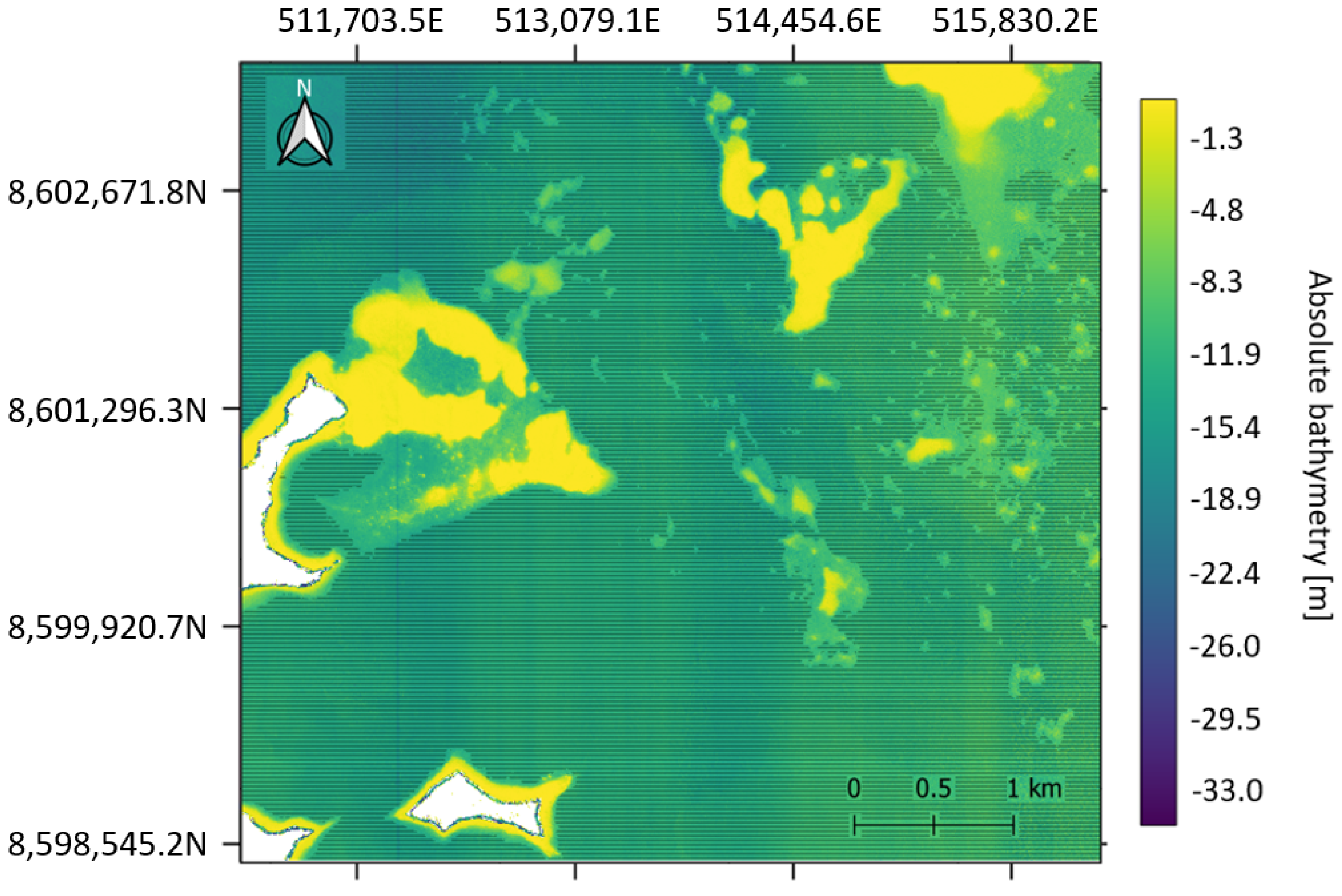
3.1.3. Digital Depth Model

ICESat-2 corrected and validated data were used to calibrate the relative DDM. The calibration required the identification of a good model to bound the ICESat-2 dataset to the relative water depth values from the 0.5 m MS imagery.

Scaled pixel values were extracted from the relative water depth map derived from the 0.5 m MS imagery at the same location than ICESat-2 bathymetric points using QGIS 3.18.3 (open-source geographic information system). Several regression models were tested, and the corresponding equations and their performance (in terms of the RMSE) are presented in Figure A1 (Appendix A). The regression chosen is a 2nd degree polynomial (Equation (6)). The expression of the latter is simple and performs well, with a RMSE of 0.895 m (see Figure 8).

$$\mathrm{y}=-45.87{\mathrm{x}}^2+74.567\mathrm{x}-31.581$$

(6)

Figure 9 shows the final DDM obtained using ENVI through the application of the model to the relative DDM. The hatched areas correspond to depths greater than the maximum calibration depth.

3.1.4. Digital Depth Model Validation

The reliability of the DDM was quantified by comparing the estimated bathymetry to the Litto3D^® reference dataset. Points from the bathymetric LiDAR point clouds were extracted, along the path of ICESat-2, from the DDM. The predicted RMSE was 0.895 m and the observed RMSE was 0.874 m along the ICESat-2 path. The predicted R² coefficient was 0.931 and the observed R² coefficient was 0.97. In addition, we report a MAE of 0.701 m.

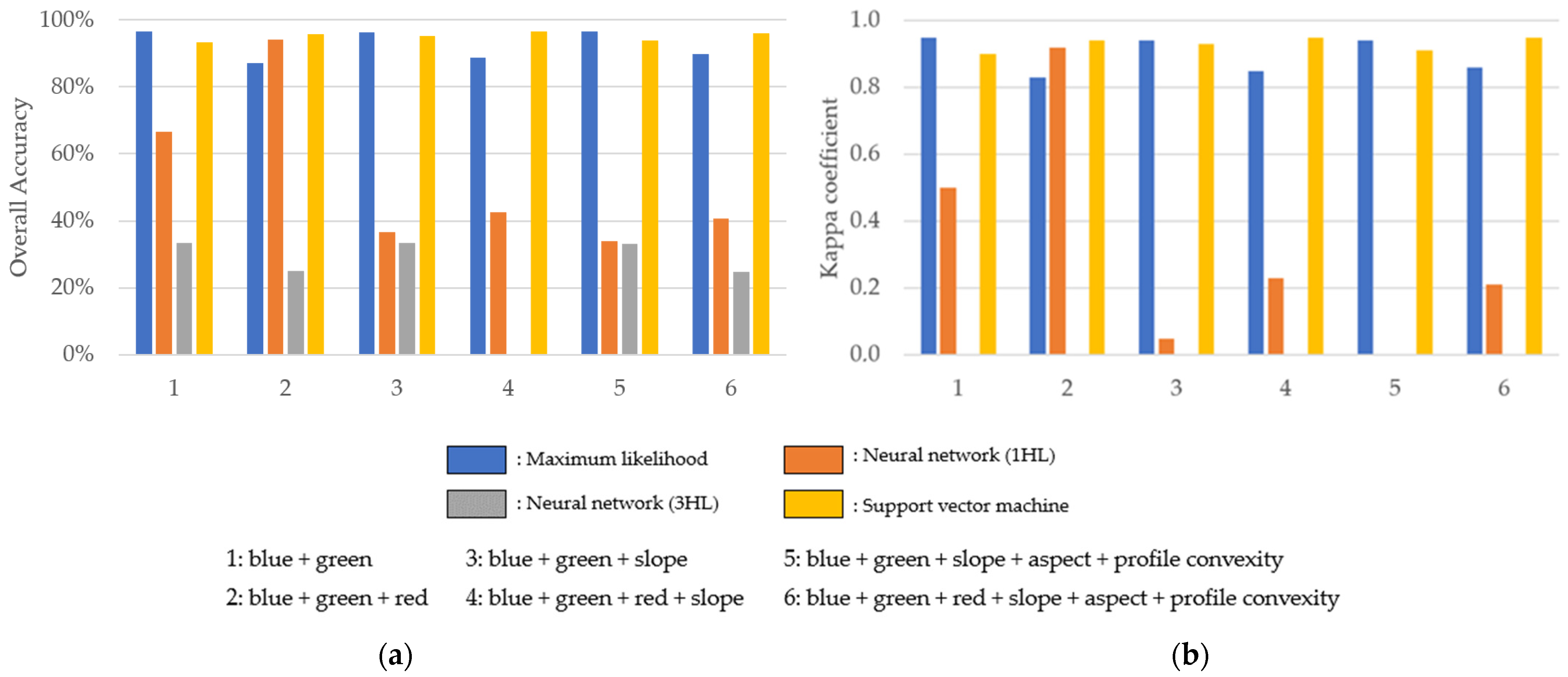
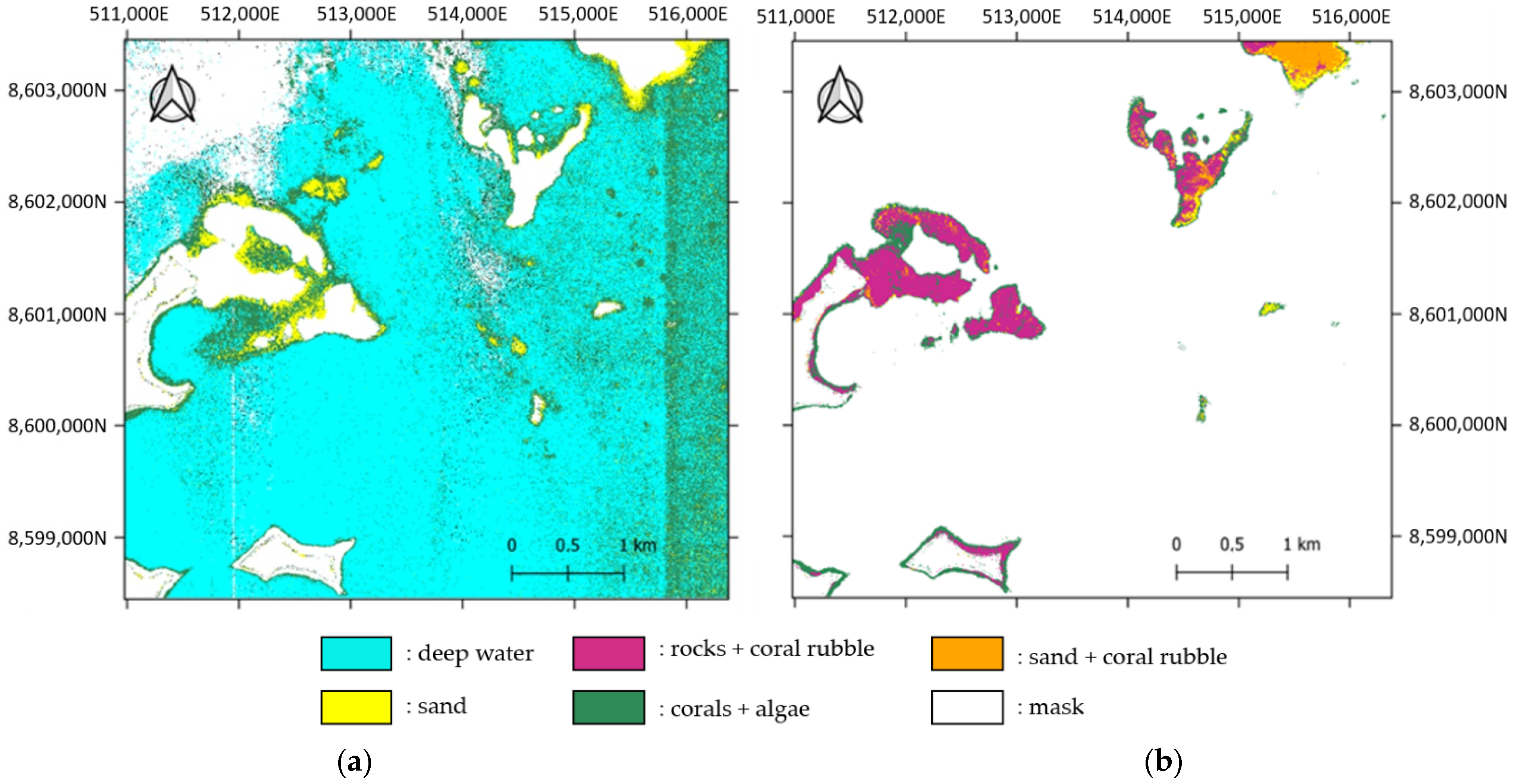
3.2. Benthic Habitat Classification

Results from the four classifiers tested using different combinations of predictors are summarized in Figure 10, presenting both the overall accuracy and the kappa coefficient values.

The NN algorithm configured with three hidden neurons for one layer systematically provided the lowest accuracy and the lowest kappa score with an overall accuracy which does not exceed 33.33% and kappa coefficient values that are all null. The neural network using only one hidden neuron produced better, yet inconclusive results, except for the combination of predictors “2”.

The ML and the SVM algorithms generally produced the best classification results. The ML algorithm allows for a global accuracy of 96.62% and a kappa coefficient of 0.94 when using two spectral bands (Green and Blue) and with the addition of the three geomorphic predictors.

The SVM results were not as affected by the absence of the red spectral band. The results are constant and reached an overall accuracy of 96.50% and a kappa coefficient of 0.95 when using a DAM with three spectral bands and the slope as the only geomorphic predictor.

Maps of the benthic habitats with the best classification results for each depth range, are presented in Figure 11.

These results, compared to the 0.5 m MS imagery and the DAM, are consistent with the classification presented in Figure 5, except for a bias in the classification of corals and algae, appearing in Figure 11a. The green band on the right of the image is an error in the classification process.

4. Discussion

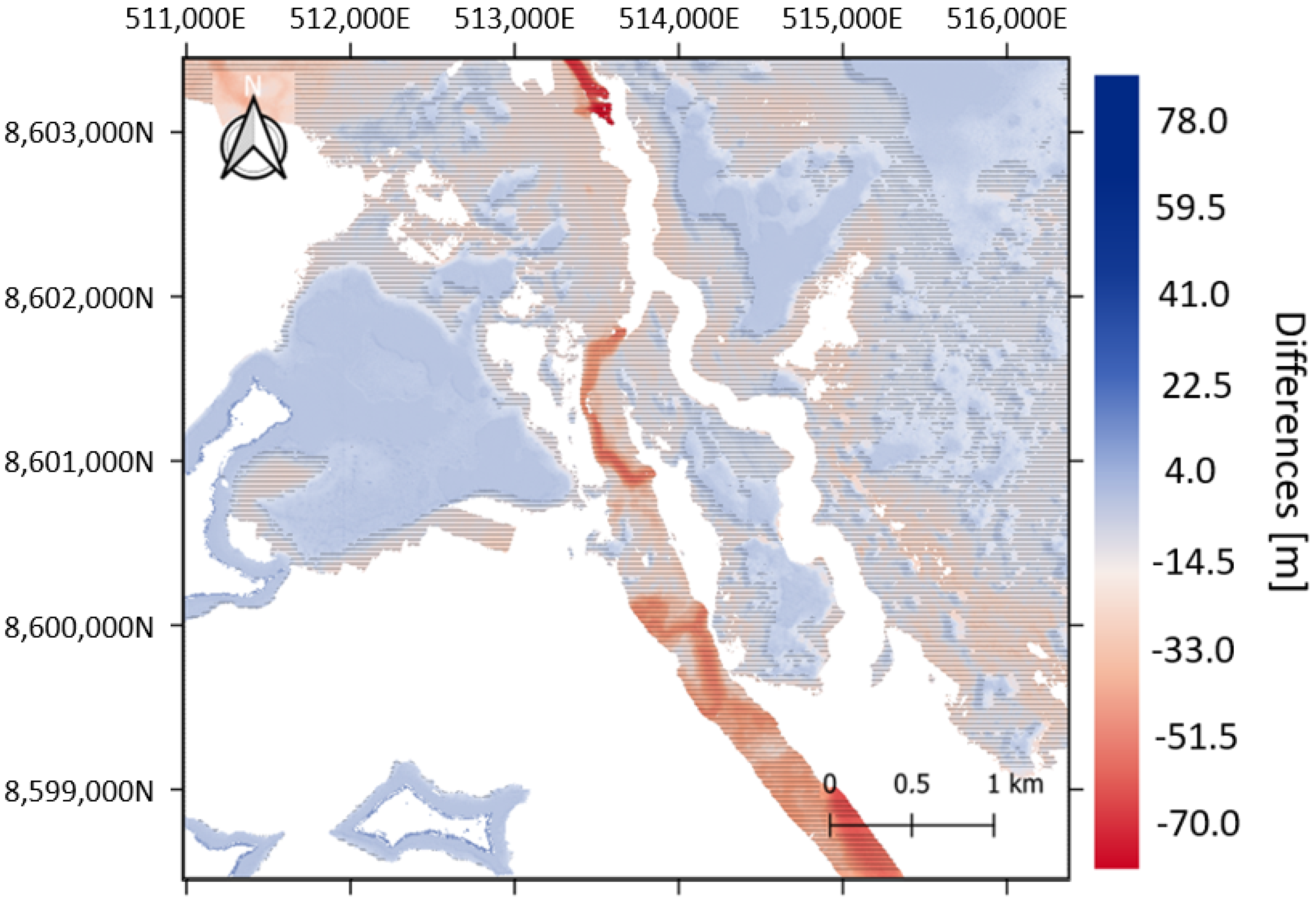
4.1. Bathymetric Errors

RMSE values comparing the DDM to the Litto3D^® dataset were obtained along the ICESat-2 ground track, thus at the same place used for the calibration. Here, we discuss the impact of both the depth values and the location of the validation transect on the results.

Figure 12 shows the DDM from the Litto3D^® dataset. While the DDM produced in our study reaches 33 m depth, the Litto3D^® survey of this area indicated depths reaching at least 82 m.

The map of the differences between the Litto3D^® and the DDM calibrated with ICESat-2 dataset is shown in Figure 13. The extrapolation works very well over the range of depths used in the calibration. However, the error increases at deeper depths. Once again, in this figure, the hatched areas correspond to depths greater than the maximum calibration depth of the model.

Large error values seem to appear in deeper waters (over 15 m depth), probably due to the fact that the bathymetry was calibrated with a limited depth range (the ICESat-2 dataset does not exceed a depth of 15 m). On the other hand, the fact data sampling was restricted to the ICESat-2 track is not ideal for the calibration. Most of the soundings represent a depth lower than 5 m (this concerns nearly 85% of the total amount of points for the 2020 dataset). The dataset only has a few points representing higher depth values. This was confirmed by the study of three other transects, taken at different places over the area (a transect along the ICESat-2 swath, a transect perpendicular to the swath, and a transect extracted far from the swath). The results of those tests are visible in Figure A2, Figure A3 and Figure A4 (Appendix B), showing that depth strongly affects the quality of the bathymetry. Consequently, errors increase for depth exceeding around 15 m. However, for shallower depth values, the results are similar, regardless of the transect location.

The 10-year difference in the time of acquisition between Litto3D^® and ICESat-2 could also induce a systematic error, due to a change in the bottom topography caused, for instance, by erosion or a change in the mean sea level (MSL), although those changes are likely to be well beyond the vertical accuracy provided by the method.

Mayotte has been prone to a succession of earthquakes since May 2018. The origin of these earthquakes is located to the east of the island. There are four permanent GPS stations in Mayotte and their rigorous monitoring has allowed experts to observe a displacement of all the stations by several centimeters towards the East and a subsidence of several centimeters since the beginning of the events [54,55,56].

In addition, the conversion of datums, using CIRCE software, could be a source of error. The grid used for the calculation is the GGM04V1 and the resulting vertical accuracy is estimated by the software at 10/20 cm.

On the other hand, during the correction of the refraction effect, n₁ and n₂ refractive indices were assumed and could therefore contribute to a small bias.

The method used to retrieve the map of the relative water depth could be improved to obtain more accurate DDM by implementing more recent and innovative approaches, such as IMBR, OBRA, MODPA or SMART-SDB [11,24,57,58,59].

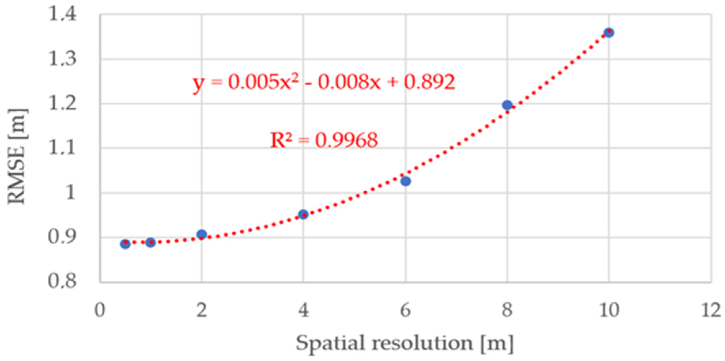
4.2. Impact of the Spatial Resolution of the Multispectral Imagery

In this study, the DDM was generated at the VHR of 0.5 m. However, other studies used sensors providing a spatial resolution of 10 m (Sentinel-2) or 30 m (Landsat-8) [17,39,60]. The spatial resolution drawn from the Pleiades-1A sensor was degraded in order to compare the RMSE. This process was done in ENVI with the “Resize Data” tool. The pixel size of the output was set according to the desired spatial resolution. The results are presented in Figure 14 and

Table 4. Accuracy using the original image resolution and lower spatial resolution.

Spatial Resolution [m]	RMSE [m]
0.5	0.89
1	0.89
2	0.91
4	0.95
6	1.03
8	1.20
10	1.36

.

Figure 14 highlights the importance of the imagery spatial resolution on the accuracy of the bathymetry. RMSE remained under 1 m when the spatial resolution remained below 5 m, but increased rapidly after.

In other studies, the RMSE reached between 1.5 and 2 m for the Yongle atoll, located in South China [17]. It was 1.2 m on average in the Acklins islands in the Bahamas based on the Sentinel-2 MS satellite with a 10 m spatial resolution [17]. The RMSE was 0.96 m with the MS satellite Sentinel-2B (10 m spatial resolution) and 1.54 m using the Landsat-8 satellite (30 m spatial resolution) in the Virgin Islands [33]. Moreover, these study areas had a diffuse attenuation coefficient (K_d) similar to the Mayotte study area.

One of these studies obtained different results using Sentinel-2 observations and ICESat-2 observations from multiple swaths [60]. The DDM was produced with an extrapolation process conducted over the entire area with a RMSE of 3.36 m. However, when the study area was constrained between the two ICESat-2 swaths, the RMSE decreased to 0.35 m. This study area had a higher turbidity of K_d = 1.68 m⁻¹ [60].

During the acquisition time of some of these studies, meteorological events such as hurricanes occurred and could have impacted the topography of the bottom and affected the results. However, the evaluation of possible episodic events was not reported for this study or investigated.

4.3. Benthic Classification

Classification algorithms performed very differently. It is difficult to assess the impact of the geomorphic predictors on the results. It seems that adding extra information did not impact the SVM and ML classifications, but could have degraded the NN (+1HL) classification. A large amount information could have undermined the results due to a redundancy in the information. The major change seems to be related to the use of the red spectral band. The results were sometimes better without the red spectral band, probably due to the fact that the corresponding maps were in the depth range of 3.7–15 m, for which benthic classes, such as sand and coral rubble and rocks and coral rubble, are not present. A reduced number of groups tends to enhance the algorithm performance.

The benthic classification is based on a visual recognition of general benthic classes based on experts’ knowledge. Although, commonly done, identifying benthic classes on MS imagery is not as reliable as direct underwater observations. Living corals could have been confused for dead corals colonized by algae. As a matter of fact, the classification presented in Figure 11a presented very good results, while having a major bias in the classification of coral and algae in areas of deep water. Some regions selected both to train the algorithm and for further validation presented corals which were distinguishable but very dark, due to the depth. Those were confused with deep and dark water areas.

Moreover, Mayotte is a complex area. The tidal range reaches 4 m. Therefore, when the tide is the lowest, corals can be above the water surface and bleached. Dead corals are theoretically recognizable by their bright color, but they can get darker as they are often colonized by algae. The winds and the waves have the effect to break coral colonies and to create coral rubble areas which are difficult to identify, as they get mixed with sand and rocks and can be mixed up with areas of isolated corals.

5. Conclusions

This study aimed to evaluate the quality of VHR DDM and DAM generated from satellite data. A DDM calibrated with data from the satellite ICESat-2 presented a RMSE of 0.89 m along ICESat-2 ground track, i.e., around 6% of the maximum depth retrieved by ICESat-2. Bathymetric results were generally satisfying down to a depth of around 15 m, which is close to the maximum depth of the calibration data used. Marine habitat classification results were very heterogeneous, depending on the number of predictors used, the type of predictors, and the algorithm used. However, some combinations of parameters provided satisfactory results. The classification with the ML classification using Blue and Green spectral bands with the three geomorphic predictors provided an overall accuracy of 96.62% and a κ coefficient of 0.94. In addition, the SVM classification using Blue, Green, and Red spectral bands with the addition of the slope geomorphic predictor presented an overall accuracy of 96.50% and a κ coefficient of 0.95. This approach can be of strong interest to map coastal areas lacking bathymetry and marine habitat maps and for which field observations are difficult.

While the quality of the results obtained in this study can support coastal management and conservation, the accuracy of bathymetry predictions remains limited for applications, such as navigation, that require higher spatial accuracy. It would be interesting to pursue this research to get more accurate DDMs.

Further work, implementing this method on diverse study sites, would confirm the robustness of the method implemented. In the prospect of future studies, it would be relevant to consider several ICESat-2 ground tracks from the area of interest and even to add the points from other times that ICESat-2 surveyed the area. This would provide a better variability of depths and a better spatial distribution of the data for the calibration process. Moreover, this increase in the number of points opens prospects for the use of deep learning methods to generate DDMs.

Developing an algorithm dedicated to the processing of seafloor data generated from ICESat-2 datasets would be important. The correction for the refraction effect has proven necessary and reliable, but could be further enhanced. The water column properties are changing with depth and the refraction correction should also adapt according to the water column properties.

It would be relevant to also improve the seabed signal correction by considering the state of the sea (for instance, presence of waves on the water surface), in helping to develop a method that could be used in less sheltered areas [17].

In this study, the results presented were obtained using a MS imagery acquired by the Pleiades-1A sensor with four spectral bands and a VHR of 0.5 m using the panchromatic band. The correlation between spatial resolution and the quality of the resulting bathymetry has been demonstrated in this paper. Therefore, future studies could consider generating better quality DDMs using the WV3 sensor (eight spectral bands at 0.30 m using the panchromatic band) or even the sensor of the new Pleiades Neo constellation launched in early 2021 (six spectral bands at 0.3 m with the panchromatic band).

The ICESat-2 products produced by NASA are constantly enhanced and one can be very optimistic regarding the future quality of DDMs and by-products obtained using ICESat-2 measurements.

References

1. Lionel, G.; Salvat, B. Coral reefs in French overseas territories: A retrospective study of changes in health conditions of these diversified and vulnerable ecosystems recorded by monitoring networks. Rev. Ecol. 2008, 63, 13–22. [Google Scholar]
2. Baker, E.; Harris, P. Habitat mapping and marine management. In GeoHab Atlas of Seafloor Geomorphic Features and Benthic Habitats, 2nd ed.; Baker, E., Harris, P., Eds.; Elsevier: Amsterdam, The Netherlands, 2020; pp. 17–33. [Google Scholar]
3. Quod, J.-P.; Dahalani, Y.; Bigot, L.; Nicet, J.B. Status of coral reefs at Réunion, Mayotte, Madagascar. In Coral Reef Degradation in the Indian Ocean; Wilhelmsson, D., Obura Olof Linden, D., Souter, D., Eds.; CORDIO SAREC Marine Science Program: Kalmar, Sweden, 2002; pp. 185–189. [Google Scholar]
4. Collin, A.; Andel, M.; Lecchini, D.; Claudet, J. Mapping Sub-Metre 3D Land-Sea Coral Reefscapes Using Superspectral WorldView-3 Satellite Stereoimagery. Oceans 2021, 2, 315–329. [Google Scholar] [CrossRef]
5. Dierssen, H.; Theberge, A. Bathymetry: Assessing Methods. In Encyclopedia of Natural Resources; Wang, Y., Ed.; Taylor & Francis Group: Abingdon-on-Thames, UK, 2014; Volume 2, pp. 1–8. [Google Scholar]
6. Collin, A.; Ramambason, C.; Pastol, Y.; Casella, E.; Rovere, A.; Thiault, L.; Espiau, B.; Siu, G.; Lerouvreur, F.; Nakamura, N.; et al. Very high-resolution mapping of coral reef state using airborne bathymetric LiDAR surface-intensity and drone imagery. Int. J. Remote Sens. 2018, 39, 5676–5688. [Google Scholar] [CrossRef] [Green Version]
7. Chen, Y.; Zhu, Z.; Le, Y.; Qiu, Z.; Chen, G.; Wang, L. Refraction correction and coordinate displacement compensation in nearshore bathymetry using ICESat-2 lidar data and remote-sensing images. Opt. Express 2021, 29, 2411–2430. [Google Scholar] [CrossRef]
8. Collin, A.; Etienne, S.; Feunteun, E. VHR Coastal bathymetry using WorldView-3: Colour versus learner. Remote Sens. Lett. 2017, 8, 1072–1081. [Google Scholar] [CrossRef]
9. Misra, A.; Vojinovic, Z.; Ramakrishnan, B.; Luijendijk, A.; Ranasinghe, R. Shallow water bathymetry mapping using Support Vector Machine (SVM) technique and multispectral imagery. Int. J. Remote Sens. 2018, 38, 1–20. [Google Scholar] [CrossRef]
10. Alevizos, E. A Combined Machine Learning and Residual Analysis Approach for Improved Retrieval of Shallow Bathymetry from Hyperspectral Imagery and Sparse Ground Truth Data. Remote Sens. 2020, 12, 3489. [Google Scholar] [CrossRef]
11. Muzirafuti, A.; Barreca, G.; Crupi, A.; Faina, G.; Paltrinieri, D.; Lanza, S.; Randazzo, G. The Contribution of Multispectral Satellite Image to Shallow Water Bathymetry Mapping on the Coast of Misano Adriatico, Italy. J. Mar. Sci. Eng. 2020, 8, 126. [Google Scholar] [CrossRef] [Green Version]
12. Eugenio, F.; Marcello, J.; Martin, J. High-resolution maps of bathymetry and benthic habitats in shallow-water environments using multispectral remote sensing imagery. IEEE Trans. Geosci. Remote Sens. 2015, 53, 3539–3549. [Google Scholar] [CrossRef]
13. Dekker, A.G.; Phinn, S.R.; Anstee, J.; Bissett, P.; Brando, V.E.; Casey, B.; Fearns, P.; Hedley, J.D.; Klonowski, W.; Lee, Z.P.; et al. Intercomparison of shallow water bathymetry, hydro-optics and benthos mapping techniques in Australian and Caribbean coastal environment. Limnol. Oceanogr. Methods 2011, 9, 396–425. [Google Scholar] [CrossRef] [Green Version]
14. Niroumand-Jadidi, M.; Bruzzone, L.; Bovolo, F. Physics-based Bathymetry and Water Quality Retrieval Using PlanetScope Imagery: Impacts of 2020 COVID-19 Lockdown and 2019 Extreme Flood in the Venice Lagoon. Remote Sens. 2020, 12, 2381. [Google Scholar] [CrossRef]
15. Gege, P. WASI-2D: A software tool for regionally optimized analysis of imaging spectrometer data from deep and shallow waters. In Computers & Geosciences; Collon, P., Grana, D., Mueller, U., Eds.; Elsevier: Amsterdam, The Netherlands, 2014; Volume 62, pp. 208–215. [Google Scholar]
16. Giardino, C.; Candiani, G.; Bresciani, M.; Lee, Z.; Gagliano, S.; Pepe, M. BOMBER: A tool for estimating water quality and bottom properties from remote sensing images. In Computers & Geosciences; Collon, P., Grana, D., Mueller, U., Eds.; Elsevier: Amsterdam, The Netherlands, 2012; Volume 45, pp. 313–318. [Google Scholar]
17. Ma, Y.; Xu, N.; Liu, Z.; Yang, B.; Yang, F.; Wang, X.; Li, S. Satellite-derives bathymetry using the ICESat-2 lidar and Sentinel-2 imagery datasets. Remote Sens. Environ. 2020, 250, 112047. [Google Scholar] [CrossRef]
18. Ashphaq, M.; Srivastava, P.K.; Mitra, D. Review of near-shore satellite-derived bathymetry: Classification and account of five decades of coastal bathymetry research. J. Ocean Eng. Sci. 2021, 6, 340–359. [Google Scholar] [CrossRef]
19. Neumann, T.A.; Martino, A.J.; Markus, T.; Bae, S.; Bock, M.R.; Brenner, A.C.; Brunt, K.M.; Cavanaugh, J.; Fernandes, S.T.; Hancock, D.W.; et al. The Ice, cloud and land elevation satellite-2 mission: A global geolocated photon product derived from the advanced topographic laser altimeter system. Remote Sens. Environ. 2019, 233, 111325. [Google Scholar] [CrossRef] [PubMed]
20. Jasinski, M.; Stoll, J.; Cook, W.; Ondrusek, M.; Stengel, E.; Brunt, K. Inland and Near-Shore Water Profiles Derived from the High-Altitutde Multiple Altimeter Beam Experimental Lidar (MABEL). J. Coast. Res. 2016, 76, 44–55. [Google Scholar] [CrossRef] [PubMed]
21. Parrish, C.; Magruder, L.; Neuenschwander, A.; Forfinski-Sarkozi, N.; Alonzo, M.; Jasinski, M. Validation of ICESat-2 ATLAS Bathymetry and Analysis of ATLAS’s Bathymetric Mappingping Performance. Remote Sens. 2019, 11, 1634. [Google Scholar] [CrossRef] [Green Version]
22. Zhang, Z.; Liu, X.; Ma, Y.; Xu, N.; Zhang, W.; Li, S. Signal Photon Extraction Method for Weak Beam Data of ICESat-2 Using Information Provided by Strong Beam Data in Mountainous Areas. Remote Sens. 2021, 13, 863. [Google Scholar] [CrossRef]
23. Stumpf, R.; Holderied, K.; Sinclair, M. Determination of water depth with high-resolution satellite imagery over variable bottom types. Limnol. Oceanogr. 2003, 48, 547–556. [Google Scholar] [CrossRef]
24. Minghelli, A.; Vadakke-Chanat, S.; Chami, M.; Guillaume, M.; Migne, E.; Grillas, P.; Boutron, O. Estimation of Bathymetry and Benthic Habitat Composition from Hyperspectral Remote Sensing Data (BIODIVERSITY) Using a Semi-Analytical Approach. Remote Sens. 2021, 13, 1999. [Google Scholar] [CrossRef]
25. Maritorena, S.; Morel, A.; Gentili, B. Diffuse reflectance of oceanic shallow waters: Influence of water depth and bottom albedo. Limnol. Oceanogr. 1994, 39, 1689–1703. [Google Scholar] [CrossRef]
26. Mishra, D.; Narumalani, S.; Rundquist, D.; Lawson, M. Benthic habitat mapping in tropical marin environments using Quickbird multispectral data. Photogramm. Eng. Remote Sens. 2006, 72, 1037–1048. [Google Scholar] [CrossRef]
27. Liew, S.; Chen, P.; Daengtuksin, B.; Chang, C. Estimating water optical properties, water depth and bottom albedo using high resolution satellite imagery for coastal habitat mapping. In Proceedings of the 2011 IEEE International Geoscience and Remote Sensing Symposium, Vancouver, BC, Canada, 24–29 July 2011; pp. 2338–2340. [Google Scholar]
28. NOAA. Available online: https://www.ngs.noaa.gov/RSD/topobathy/ (accessed on 28 December 2021).
29. Saylam, K.; Brown, R.; Hupp, J. Assessment of depth and turbidity with airborne Lidar bathymetry and multiband satellite imagery in shallow water bodies of the Alaskan North Slope. In International Journal of Applied Earth Observation and Geoinformation; Li, J., Ed.; Elsevier: Amsterdam, The Netherlands, 2017; Volume 58, pp. 191–200. [Google Scholar]
30. Caballero, I.; Stumpf, R.P.; Meredith, A. Preliminary Assessment of Turbidity and Chlorophyll Impact on Bathymetry Derived from Sentinel-2A and Sentinel-3A Satellites in South Florida. Remote Sens. 2019, 11, 645. [Google Scholar] [CrossRef] [Green Version]
31. Peeri, S.; Azuike, C.; Parrish, C. Satellite-derived bathymetry a reconnaissance tool for hydrography. Hydro Int. 2013, 17, 16–19. [Google Scholar]
32. NASA Goddard Space Flight Center, Ocean Ecology Laboratory, Ocean Biology Processing Group; 2014: MODIS-Aqua Ocean Color Data; NASA Goddard Space Flight Center, Ocean Ecology Laboratory, Ocean Biology Processing Group. Available online: https://oceancolor.gsfc.nasa.gov/l3/ (accessed on 28 December 2021).
33. Babbel, B.; Parrish, C.; Magruder, L. ICESat-2 Elevation Retrievals in Support of Satellite-Derived Bathymetry for Global Science Applications. Geophys. Res. Lett. 2021, 48, e2020GL090629. [Google Scholar] [CrossRef]
34. IGN. Available online: https://geodesie.ign.fr/contenu/fichiers/documentation/SRCfrance.pdf (accessed on 28 December 2021).
35. Global Scan Technologies. Available online: http://www.gstdubai.com/satelliteimagery/pleiades-1a.html (accessed on 28 December 2021).
36. ESA. Available online: https://earth.esa.int/web/eoportal/satellite-missions/i/icesat-2 (accessed on 28 December 2021).
37. Neumann, T.A.; Brenner, A.; Hancock, D.; Robbins, J.; Saba, J.; Harbeck, K.; Gibbons, A.; Lee, J.; Luthcke, S.B.; Rebold, T.; et al. ATLAS/ICESat-2 L2A Global Geolocated Photon Data, Version 3. [ATL03]; NASA National Snow and Ice Data Center Distributed Active Archive Center: Boulder, CO, USA, 2020. [Google Scholar]
38. Ester, M.; Kriegel, H.-P.; Sander, J.; Xu, X. A density-based algorithm for discovering clusters in large spatial databases with noise. In Proceedings of the Second International Conference on Knowledge Discovery and Data Mining (KDD’96), Portland, OR, USA, 2–4 August 1996; AAAI Press: Palo Alto, CA, USA, 1996; pp. 226–231. [Google Scholar]
39. Xie, C.; Chen, P.; Pan, D.; Zhong, C.; Zhang, Z. Improved Filtering of ICESat-2 Lidar Data for Nearshore Bathymetry Estimation Using Sentinel-2 Imagery. Remote Sens. 2021, 13, 4303. [Google Scholar] [CrossRef]
40. Xun, N.; Ma, X.; Ma, Y.; Zhao, P.; Yang, J.; Wang, H. Deriving Highly Accurate Shallow Water Bathymetry From Sentinel-2 and ICESat-2 Datasets by a Multitemporal Stacking Method. IEEE J. Sel. Top. Appl. Earth Obs. Remote Sens. 2021, 14, 6677–6685. [Google Scholar]
41. Khater, I.; Nabi, I.R.; Hamarneh, G. A Review of Super-Resolution Single-Molecule Localization Microscopy Cluster Analysis and Quantification Methods. Patterns 2020, 1, 100038. [Google Scholar] [CrossRef] [PubMed]
42. Randazzo, G.; Barreca, G.; Cascio, M.; Crupi, A.; Fontana, M.; Gregorio, F.; Lanza, S.; Muzirafuti, A. Analysis of Very High Spatial Resolution Images for Automatic Shoreline Extraction and Satellite-Derived Bathymetry Mapping. Geosciences 2020, 10, 172. [Google Scholar] [CrossRef]
43. Gabr, B.; Ahmed, M.; Marmoush, Y. PlanetScope and Landsat 8 Imageries for Bathymetry Mapping. J. Mar. Sci. Eng. 2020, 8, 143. [Google Scholar] [CrossRef] [Green Version]
44. Pe’eri, S.; Parrish, C.; Azuike, C.; Alexander, L.; Armstrong, A. Satellite Remote Sensing as a Reconnaissance Tool for Assessing Nautical Chart Adequacy and Completeness. Mar. Geodesy 2014, 37, 293–314. [Google Scholar] [CrossRef]
45. Poppenga, S.; Palaseanu-Lovejoy, M.; Gesch, D.; Danielson, J.; Tyler, D. Evaluating the Potential for Near-Shore Bathymetry on the Majuro Atoll, Republic of the Marshall Islands, Using Landsat 8 and WorldView-3 Imagery; Scientific Investigations Report 2018-5024; U.S. Geological Survey: Reston, VA, USA, 2018.
46. Favoretto, F.; Morel, Y.; Waddington, A.; Lopez-Calderon, J.; Cadena-Roa, M.; Blanco-Jarvio, A. Testing of the 4SM Method in the Gulf of California Suggests Field Data Are not Needed to Derive Satellite Bathymetry. Sensors 2017, 17, 2248. [Google Scholar] [CrossRef] [PubMed] [Green Version]
47. Nur, H.; Othman, Y.; Wiwin, W.; Saiful, S. Integration of Satellite-Derived Bathymetry and Sounding Data in Providing Continuous and Detailed Bathymetric Information. In IOP Conference Series: Earth and Environmental Science, Proceedings of the 2nd Maritime Science and Advanced Technology; Marine Science and Technology in Framework of The Sustainable Development Goals, Makassar, Indonesia, 7–8 August 2019; IOP Publishing Ltd.: Bristol, UK, 2020; Volume 618, p. 012018. [Google Scholar]
48. Yakup, D.; Zeliha, S.; Bulent, S.; Mehmet, A.; Dagdeviren, M. Determination of sediment deposition of Hasanlar Dam using bathymetric and remote sensing studies. Nat. Hazards 2019, 97, 211–227. [Google Scholar]
49. Monteys, X.; Harris, P.; Caloca, S.; Cahalane, C. Spatial Prediction of Coastal Bathymetry Based on Multispectral Satellite Imagery and Multibeam Data. Remote Sens. 2015, 7, 13782–13806. [Google Scholar] [CrossRef] [Green Version]
50. Collin, A.; Planes, S. Enhancing Coral Health Detection Using Spectral Diversity Indices from WorldView-2 Imagery and Machine Learners. Remote Sens. 2012, 4, 3244–3264. [Google Scholar] [CrossRef] [Green Version]
51. Morel, A.; Maritorena, S. Bio-optical properties of oceanic waters: A reappraisal. J. Geophys. Res. 2001, 106, 7163–7180. [Google Scholar] [CrossRef] [Green Version]
52. Mogstad, A.; Johnsen, G.; Ludvigsen, M. Shallow-Water Habitat Mapping using Underwater Hyperspectral Imaging from an Unmanned Surface Vehicle: A Pilot Study. Remote Sens. 2019, 11, 685. [Google Scholar] [CrossRef]
53. Story, M.; Congalton, R.G. Accuracy assessment: A user’s perspective. Photogramm. Eng. Remote Sens. 1986, 52, 397–399. [Google Scholar]
54. Lemoine, A.; Briole, P.; Bertil, D.; Roullé, A.; Foumelis, M.; Thinon, I.; Raucoules, D.; de Michele, M.; Valty, P.; Hoste Colomer, R. The 2018–2019 seismo-volcanic crisis east of Mayotte, Comoros islands: Seismicity and ground deformation markers of an exceptional submarine eruption. Geophys. J. Int. 2020, 223, 22–44. [Google Scholar] [CrossRef]
55. Cesca, S.; Letort, J.; Razafindrakoto, H.N.T.; Heimann, S.; Rivalta, E.; Isken, M.P.; Nikkhoo, M.; Passarelli, L.; Petersen, G.L.; Cotton, F.; et al. Drainage of a deep magma reservoir near Mayotte inferred from seismicity and deformation. Nat. Geosci. 2020, 13, 87–93. [Google Scholar] [CrossRef]
56. Feuillet, N.; Jorry, S.; Crawford, W.; Deplus, C.; Thinon, I.; Jacques, E.; Van der Woerd, J. Birth of a large volcanic edifice through lithosphere-scale dyking offshore Mayotte (Indian Ocean). Nat. Geosci 2021. under review. [Google Scholar] [CrossRef]
57. Amrari, S.; Bourassin, E.; Andréfouët, S.; Soulard, B.; Lemonnier, H.; Le Gendre, R. Shallow Water Bathymetry Retrieval Using a Band-Optimization Iterative Approach: Application to New Caledonia Coral Reef Lagoons Using Sentinel-2 Data. Remote Sens. 2021, 13, 4108. [Google Scholar] [CrossRef]
58. Niroumand-Jadidi, M.; Vitti, A.; Lyzenga, D.R. Multiple Optimal Depth Predictors Analysis (MODPA) for river bathymetry: Findings from spectroradiometry, simulations, and satellite imagery. Remote Sens. Environ. 2018, 218, 132–147. [Google Scholar] [CrossRef]
59. Niroumand-Jadidi, M.; Bovolo, F.; Bruzzone, L. SMART-SDB: Sample-specific multiple band ratio technique for satellite-derived bathymetry. Remote Sens. Environ. 2020, 251, 112091. [Google Scholar] [CrossRef]
60. Albright, A.; Glennie, C. Nearshore Bathymetry From Fusion of Sentinel-2 and ICESat-2 Observations. IEEE Geosci. Remote Sens. Lett. 2021, 18, 900–904. [Google Scholar] [CrossRef]
Figure 1. Map of the ground tracks of ICESat-2 over Mayotte collected on 14 May 2020. The satellite multispectral imagery was acquired by Pleiades-1A on 25 May 2020. The red square identifies the study area.
Remotesensing 14 00133 g001
Figure 2. Photon point clouds of the transect along ICESat-2 gt1l (strong beam), acquired on 14 May 2020. The confidence levels provided by ATL03 are displayed.
Remotesensing 14 00133 g002
Figure 3. (a) Schematic diagram for the change of coordinate systems and the computation of the refraction bias in the horizontal plane; (b) in the vertical plane (figure adapted from [21]); and (c) correction formulas.
Remotesensing 14 00133 g003
Figure 4. Variables involved in the process of retrieving ICESat-2 bathymetry at the acquisition time of Pleiades-1A.
Remotesensing 14 00133 g004
Figure 5. Maps of the five benthic habitats identified on the 0.5 m Pleiades-1A TOA reflectance imagery.
Remotesensing 14 00133 g005
Figure 6. Point clouds of the ICESat-2 signal acquired on 14 May 2020. The signal was processed to remove the noise, correct for refraction, and identify the seafloor. Uncorrected seafloor photons appear in red, while corrected photons are in green.
Remotesensing 14 00133 g006
Figure 7. Point clouds of Litto3D® dataset (blue), and ICESat-2 raw (yellow) and corrected (red) seabed photons.
Remotesensing 14 00133 g007
Figure 8. (a) Relative DDM with superposition of ICESat-2 bathymetric points; (b) 2nd degree polynomial regression.
Remotesensing 14 00133 g008
Figure 9. Digital depth model at the acquisition time of Pleiades-1A, calibrated with the ICESat-2 dataset.
Remotesensing 14 00133 g009
Figure 10. Performances of the different classifiers using different geomorphological predictors. (a) Overall accuracy; (b) Kappa coefficient.
Remotesensing 14 00133 g010
Figure 11. Maps of benthic habitats in the study area. (a) Classification map generated using the SVM with the slope geomorphic predictor. This map corresponds to depths shallower than 3.8 m and is based on all three spectral bands (R, G, and B); (b) classification map generated with the ML classifier and the three geomorphic predictors. This map corresponds to depths in the range of 3.8–15 m and is based on two spectral bands (G and B).
Remotesensing 14 00133 g011
Figure 12. Digital depth model generated from the Litto3D® dataset acquired over Mayotte and centered on the study site. The land area is masked.
Remotesensing 14 00133 g012
Figure 13. Map of the differences between the DDM derived from the Litto3D® and the ICESat-2/Pleiades-1 fusion.
Remotesensing 14 00133 g013
Figure 14. Performances of the DDMs obtained from different spatial resolutions of Pleiades-1A and calibrated with ICESat-2.
Remotesensing 14 00133 g014