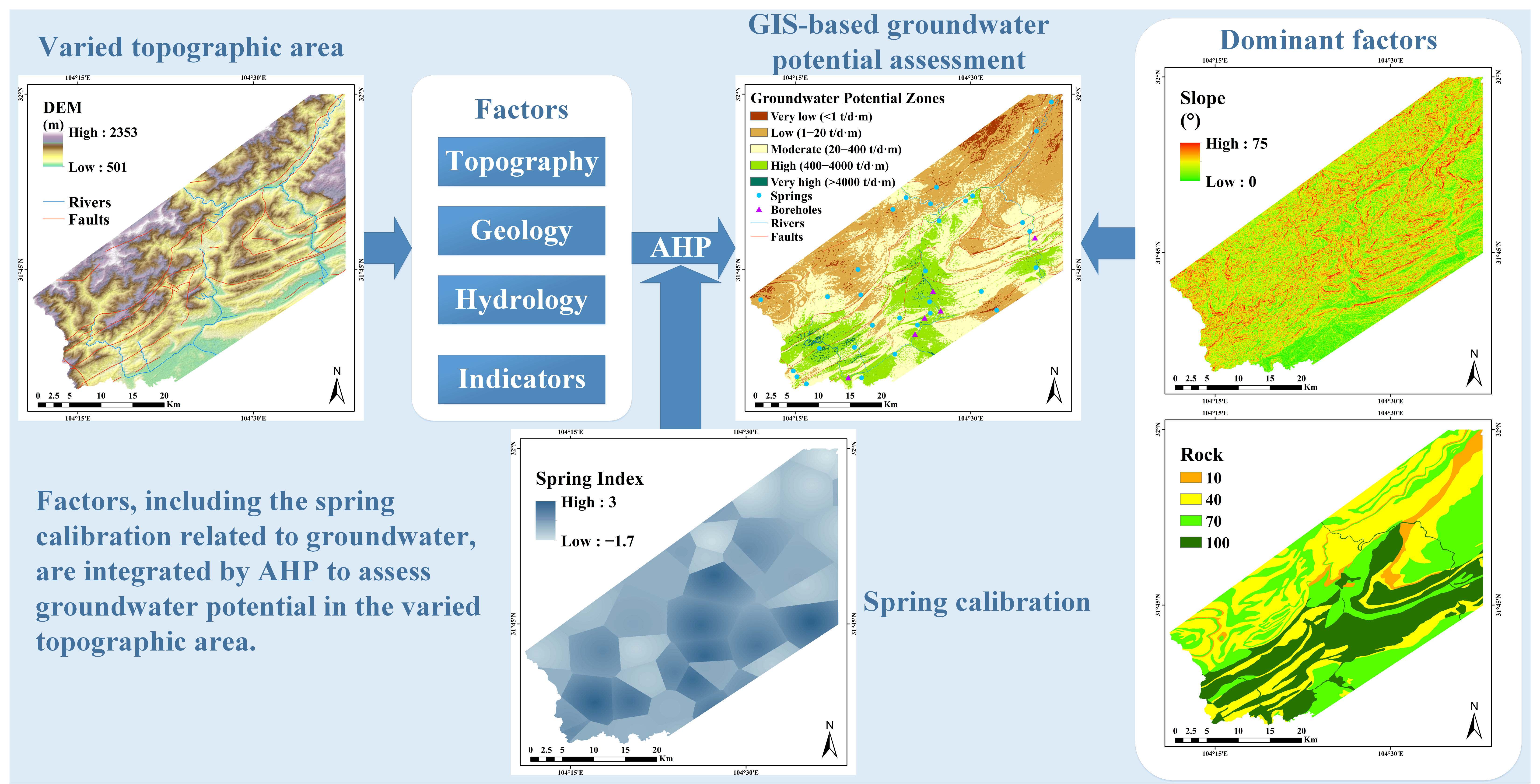
GIS-Based Groundwater Potential Assessment in Varied Topographic Areas of Mianyang City, Southwestern China, Using AHP

Abstract

Mianyang City is located in the varied topographic areas of Sichuan Province in southwestern China and is characterized by a complex geological background. This area is prone to disasters and its varied topography is inconvenient for emergency water storage and supply. Groundwater is essential for alleviating the demand for water and post-disaster emergency water supply in this area. This study applied AHP to integrate remote sensing, geological and hydrological data into GIS for the assessment of groundwater potential, providing a plan for the rational exploitation of groundwater and post-disaster emergency water supply in the area. Nine factors, including the spring calibration related to groundwater, were integrated by AHP after multicollinear checks. As a result, the geology-controlled groundwater potential map was classified into five levels with equal intervals. All the results were validated using borehole data, indicating the following: the areas with yield rates of $<1\mathrm{t}/\mathrm{d}·\mathrm{m}$, 1–20 $\mathrm{t}/\mathrm{d}·\mathrm{m}$, and 20–400 $\mathrm{t}/\mathrm{d}·\mathrm{m}$ accounted for 2.66%, 36.1%, and 39.62%, respectively, whereas the areas with yield rates of 400–4000 $\mathrm{t}/\mathrm{d}·\mathrm{m}$ and $>4000\mathrm{t}/\mathrm{d}·\mathrm{m}$ accounted for only 20.88% and 0.75% of the overall area. The flexibility of this quick and efficient method enables its application in other regions with a similar geological background.

1. Introduction

Groundwater is a valuable resource that is crucial for ecosystems and human civilization, but population growth and agricultural expansion are placing increasing pressure on groundwater resources that need to be managed rationally [1,2]. Mianyang City is a varied topographic area of Sichuan Province in southwestern China. Several disasters, such as earthquakes and landslides, have occurred in the area due to strong tectonic activity [3]. The topography of the area makes the fast and efficient demand of emergency water storage and supply necessary. Groundwater serves as an important source of water and can effectively meet this demand [4], which is a key emergency water supply resource during post-disaster reconstruction processes [5]. One of the most valuable advantages of groundwater is that it is less susceptible to environmental contamination than surface water, which is very helpful for both emergency water supply and domestic drinking water [6]. However, the thorough exploration of groundwater resources is difficult due to the economic and transportation conditions in the topographic areas where considerable groundwater resources remain underutilized [7]. Therefore, assessing local groundwater potential is essential for sustained development.

Groundwater exploration in the varied topographic area in the central part of Mianyang City, Sichuan Province, is a challenging task (Figure 1). Traditionally, drilling tests and hydrogeological investigations have been widely used [8,9]. These methods are suitable for identifying the characteristics of groundwater; however, they are very costly and time-consuming as a means of establishing the distribution of groundwater resources in a large-scale region [10,11,12]. Furthermore, groundwater can be monitored indirectly using remote sensing (RS) techniques [13]. RS techniques offer repetitive coverage of an area with the combination of different ranges of the electromagnetic spectrum, and they are useful for obtaining spatiotemporal data of sizable areas in a short interval [14,15,16]. RS not only provides high-precision spatial-temporal observations, but also characterizes features on the Earth’s surface, such as geomorphology and drainage patterns [17]. As a result, RS has recently become popular for groundwater assessment because it can produce quick and suitable guidelines and information about the occurrences and movements of groundwater [11,18].

Geographic information systems (GIS) are computer applications designed for the acquisition, storage, analysis, modeling, archiving, and sharing of geographic information [19]. GIS is a powerful tool for handling a massive amount of spatial data and can be used in the decision-making process, based on which hydrologists can extract reasonable variables to evaluate groundwater potential. Exploration using the integration of RS and GIS has gained special attention recently because it is an economic and efficient method [20,21]. Meanwhile, researchers have applied various methods of multiple-criteria decisions to identify the impact of different factors in GIS-based groundwater assessments [22,23], such as frequency ratios [24,25], random forest [26,27], logistic regression [28,29], neural network [30,31], and fuzzy logic [32,33]. Methods such as frequency ratios and neural networks exhibit high accuracy, but they require a large amount of groundwater information in the study area and are poorly applicable with insufficient data [34,35]. The evaluation accuracy of machine learning methods such as random forest and neural network is affected by the number and selection of mass samples, whereas the inherent reasoning process and basis are difficult to explain [36]. Compared with the above methods, the analytical hierarchical process (AHP) adopted in the present study is another reliable and convenient method to delineate groundwater potential zones with a moderate amount of data. AHP allows for the hierarchical structuring of decisions (to reduce their complexity) and shows relationships between objectives (or criteria) and possible alternatives [37,38]. AHP has clear decision criteria and a transparent decision process, which makes it easy to share the decision process as a reference for other regions; it can also rely on rich experience to reveal the characteristics of groundwater accurately [39,40]. Several studies [41,42,43,44] have used AHP to determine the weights of factors based on a priori information and various conditions. The present study firstly tried to use AHP to assess a varied topographic area with a complex geological background, assimilating the RS data, spring data, and other available geological data. Multiple factors related to the occurrence, origin, distribution, and movement of groundwater were established based on these data to reduce the limitation of single data and improve the accuracy of the assessment.

When assessing groundwater in varied topographic areas, the selection of factors in current studies is considered as geology (e.g., lithology, soil type), topography (e.g., slope, drainage density), and groundwater recharge (e.g., rainfall) [43,45,46]. Some studies also include indicators related to groundwater (e.g., normalized difference vegetation index (NDVI), land-use land-cover (LULC)) [24,33], whereas factors of fault lineament are also included as geological conditions [22,27]. However, these factors reflect groundwater indirectly, and the transformation between surface water and groundwater is not fully understood. For reasonable assessment, seven factors from previous studies (rock, fault density, slope, convergence index, drainage density, rainfall, and distance from rivers) are all adopted, as is the enhanced vegetation index (EVI), which is a special factor in this varied topographic area. The spring index, which is a visual representation of groundwater conditions, is also innovatively established by assimilating actual spring data.

The purpose of this study was to conduct a detailed groundwater potential assessment of varied topographic areas with complex geological backgrounds based on previous studies and investigations. Additionally, it aimed to identify the important factors affecting groundwater potential. Based on the collected data, including RS data, hydrological and geological data, GIS was used to establish an AHP-based method for mapping groundwater potential. Multicollinear checks and borehole-data standardization were used to validate the results. Reasonable assessment and verification may ensure a reference for sustainable groundwater development and the prudent management of emergency water supplies.

2. Materials and Methods

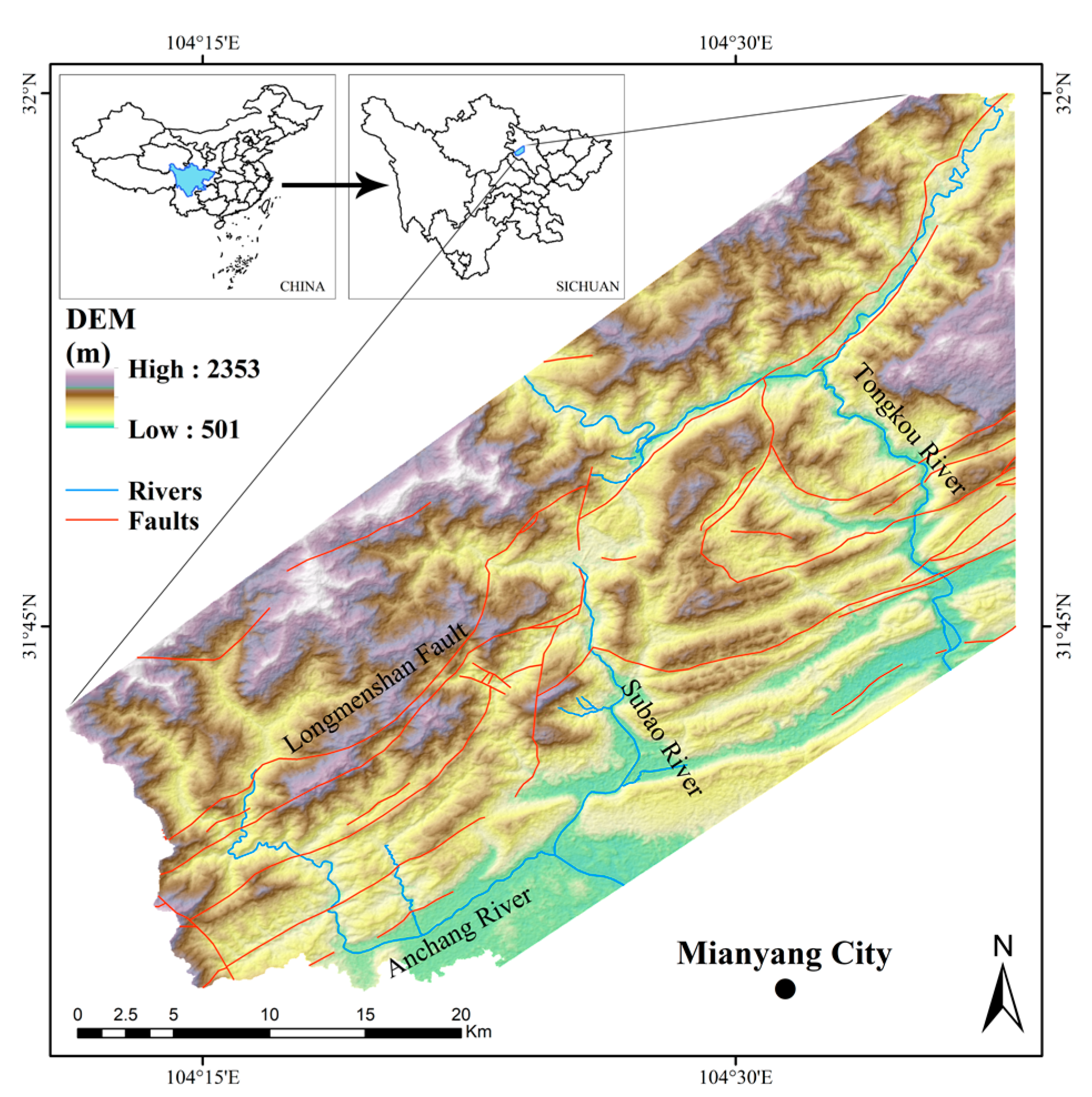
Based on the conventional geological, RS, and hydrological data in this varied region, nine factors were taken into account: rock, fault density, spring index, slope, drainage density, EVI, convergence index, rainfall, and distance from rivers. The weights of each factor were determined using the AHP method after a multicollinear check. A groundwater potential map was generated using overlay analysis and further validated with borehole data. The methodology used to evaluate groundwater potential is illustrated in Figure 2.

2.1. Study Area

The study area is located in central Mianyang City, Sichuan Province, China (Figure 1). Its longitude range is from $104°{11}^{\prime }\mathrm{E}$ to $104°{38}^{\prime }\mathrm{E}$, and the latitude range is from $31°{34}^{\prime }\mathrm{N}$ to $32°\mathrm{N}$. The elevation ranges from a high of 2345 m in the northwest to a low of 501 m in the southeast. The area is dominated by the northeast-oriented Longmenshan Fault, with the Songpan-Ganzi Fold System in the west and the Sichuan Basin in the east. Complex tectonic deformation has weakened the tectonic stress field in the region [47]. According to the hydrogeological map obtained from the Geological Environment Monitoring Institute of China Geological Survey, a large carbonate karst fissure of water is distributed in the central part, and bedrock fissure water is mainly distributed in the northwest of the fracture zone; unconsolidated strata pore water and clastic fracture water are mostly distributed in the northeast and south (Figure 3) [48].

The area experiences a humid, subtropical climatic condition with a mean annual temperature of 16 °C and annual rainfall of over 1100 mm. Three Fujiang River tributaries flow through the area, namely, the Anchang River, the Subao River, and the Tongkou River.

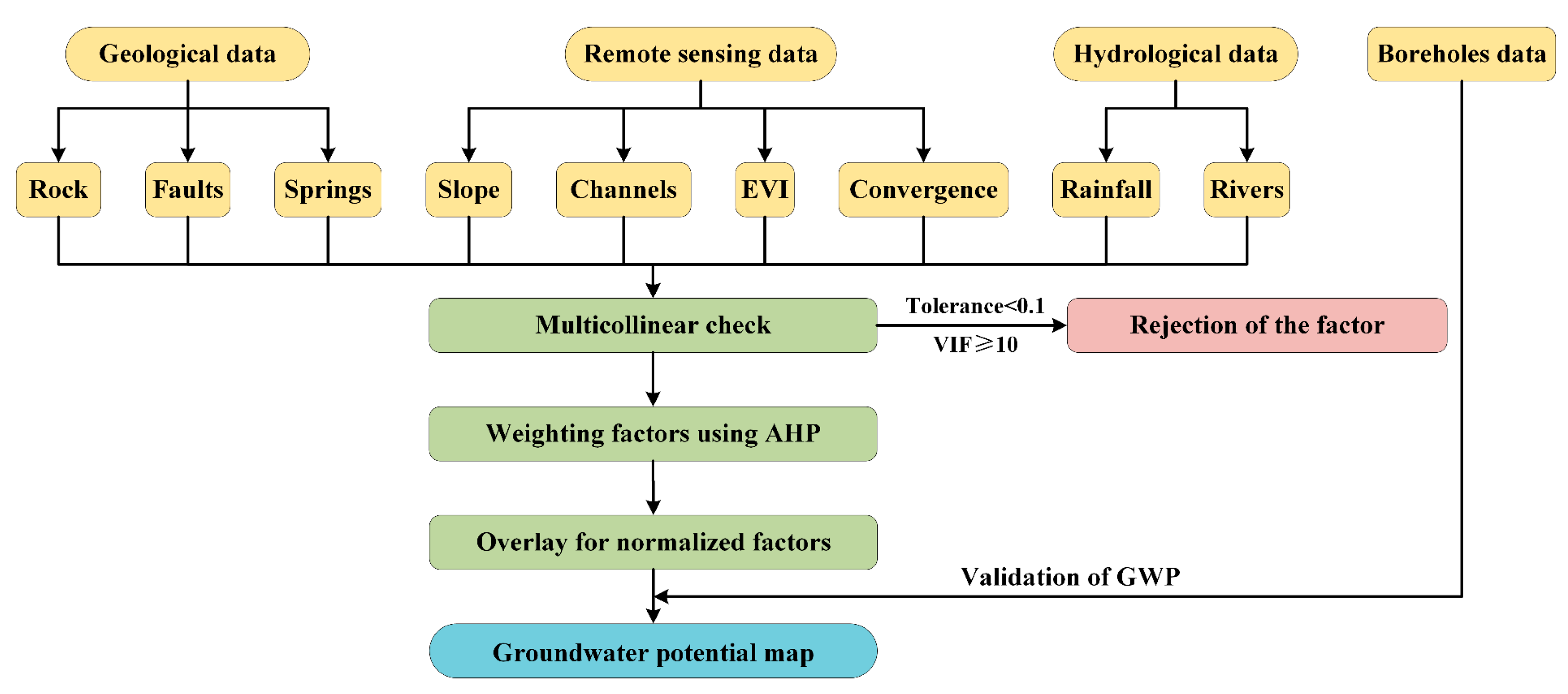
2.2. Evaluation Method

2.2.1. Weighting Method and Overlay Analysis

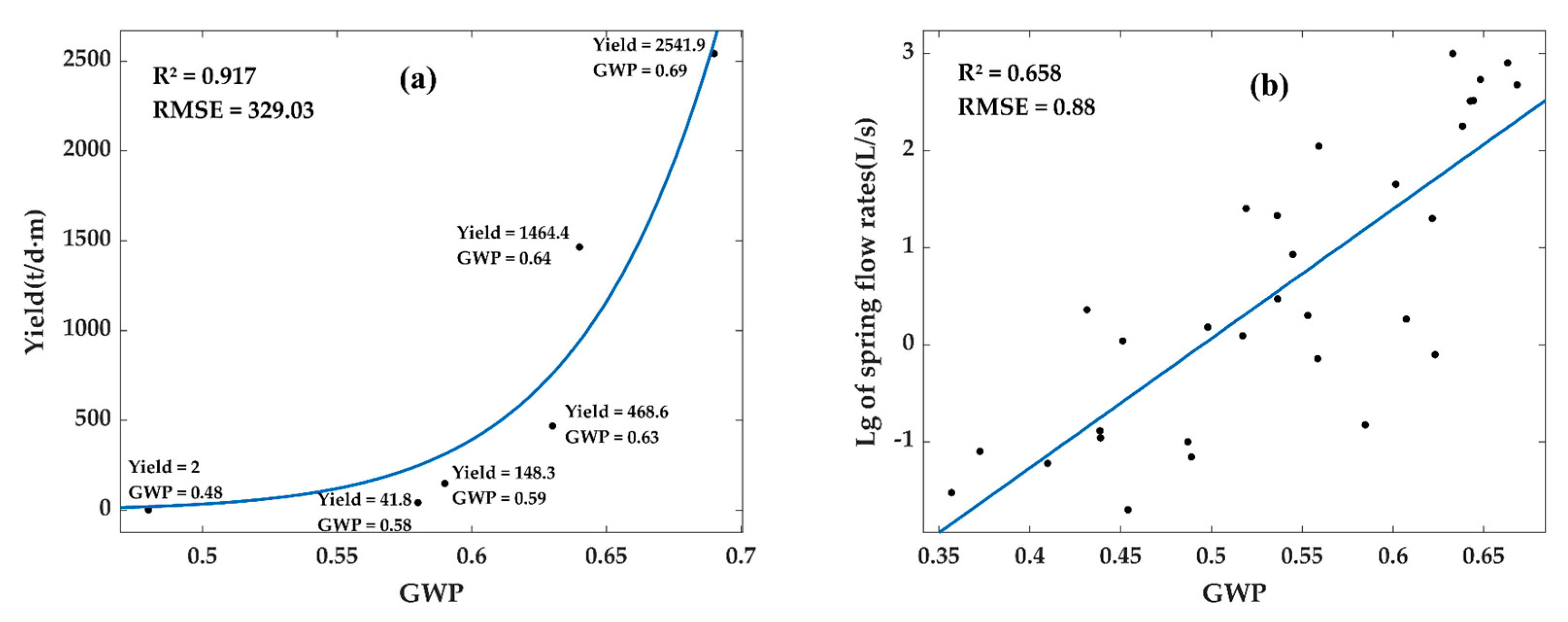
AHP, a useful multicriteria decision-making method, was used to assign weights to each established factor for reasonable assessment [39]. We used previous knowledge to categorize the occurrence and movement of groundwater hierarchically and examine it through the AHP technique [49]. The following steps were adapted to assign weights of the factors using the AHP technique: (1) defining the goal (groundwater potential); (2) deciding the factors about the occurrence and movement of groundwater and defining scaled weights for each factor according to Saaty’s scale from 1 to 9 (

Table 1. Saaty’s scale of preference between two factors in AHP.

Scale	Degree of Preference	Description
1	Equally	When two parameters contribute equally to the objective
2	Intermediate	Preference between 1 and 3
3	Moderately	The judgment slightly to-moderately favor one parameter
4	Intermediate	Preference between 3 and 5
5	Strongly	The judgment strongly or essentially favors one parameter
6	Intermediate	Preference between 5 and 7
7	Very strongly	Very strong preference or importance
8	Intermediate	Preference between 7 and 9
9	Extremely	Quite preferred or quite important

); (3) establishment of pairwise comparison metric based on the relative scale weights of selected factors; (4) calculating the geometric mean of pairwise comparison matrix; (5) calculating the inconsistency index; (6) obtaining the overall derived weights to the factors. The comparison scale weight ratings are on a scale of 1–9. The normalized weights of all factors were examined for the consistency ratio (CR) [40,50,51].

The AHP pairwise comparison metric was developed as:

$$\mathrm{M}=[\begin{array}{cccc}{m}_{11}& m_{12}& \dots & m_{1n}\\ m_{21}& m_{22}& \dots & m_{2n}\\ ⋮& ⋮& \ddots & ⋮\\ m_{n1}& m_{n2}& \dots & m_{nn}\end{array}]$$

(1)

where $m_{nn}$ represents the relative scale weight of pairwise factors.

The normalized weights were calculated from the matrix as:

$${\mathrm{W}}_{\mathrm{n}}=\left(\frac{{\mathrm{GM}}_{\mathrm{n}}}{{{\displaystyle \sum }}_{\mathrm{n}=1}^{\mathrm{N}}{\mathrm{GM}}_{\mathrm{n}}}\right)$$

(2)

where ${\mathrm{GM}}_{\mathrm{n}}$ indicates the geometric mean of nth row elements which were calculated as:

$${\mathrm{GM}}_{\mathrm{n}}=\sqrt{{\mathrm{m}}_{1\mathrm{n}}{\mathrm{m}}_{2\mathrm{n}}\cdots {\mathrm{m}}_{\mathrm{nN}}}$$

(3)

The weights obtained from pairwise comparisons were verified based on consistency ratio (CR) as [40]:

$$\mathrm{Consistency}\mathrm{Ratio}\left(\mathrm{CR}\right)=\frac{\mathrm{Consistency}\mathrm{Index}\left(\mathrm{CI}\right)}{\mathrm{Random}\mathrm{Consistency}\mathrm{Index}\left(\mathrm{RCI}\right)}$$

(4)

The random consistency index values originate from Saaty’s standard, as listed in

Table 2. Saaty’s consistency indices of randomly generated reciprocal matrices.

Order of the Matrix	1	2	3	4	5	6	7	8	9
RCI	0	0	0.58	0.90	1.12	1.24	1.32	1.41	1.45

. The consistency index values were calculated using:

$$\mathrm{CI}=\frac{{\mathsf{\lambda }}_{\max }-\mathrm{n}}{\mathrm{n}-1}$$

(5)

where ${\mathsf{\lambda }}_{\max }$ is the principal eigenvalue calculated through the eigenvector calculation process. A CR of $\le 0.1$ indicates that the AHP analysis should be continued, and if CR $>0.1$, it is necessary to modify the evaluation to determine the cause of inconsistency and then correct it (until CR $\le 0.1$).

After the weights had been determined, the factor was normalized and then overlaid using the weighted overlay method (spatial analyst tool) in ArcGIS to obtain the groundwater potential values as:

$$\mathrm{GWP}={{\displaystyle \sum }}_{\mathrm{i}=1}^{\mathrm{n}}\left({\mathrm{w}}_{\mathrm{i}}{\times \mathrm{v}}_{\mathrm{i}}\right)$$

(6)

where GWP is the groundwater potential value, ${\mathrm{w}}_{\mathrm{i}}$ is the weight of each factor, and ${\mathrm{v}}_{\mathrm{i}}$ is the normalized value of each factor.

2.2.2. Validation

After the factors for groundwater potential assessment were decided, the multicollinearity among these factors needed to be validated. Multicollinearity implies that at least one input parameter of a multivariate model is highly correlated with a combination of other input parameters. The results in a nontrivial degree of accuracy in the model output if one input parameter can be linearly predicted from another input parameter of the multivariate model. Thus, the multicollinear problem of all factors needed to be checked before running the regression model. To check the multicollinearity, linear regression analysis for each factor was used, where one input factor was considered as the dependent variable and the remaining input factors were considered as independent variables. The ${\mathrm{R}}^2$ value of the regression for each factor was calculated. The multicollinearity among all the factors was identified using the ${\mathrm{R}}^2$ value to calculate the tolerance and the variance inflation factor (VIF) of the given input factors as [52,53]:

$$\mathrm{Tolerance}=1-{\mathrm{R}}^2$$

(7)

$$\mathrm{VIF}=\frac{1}{\mathrm{Tolerance}}$$

(8)

${\mathrm{R}}^2$ measures the fit of the regression equation to the factors. The larger the ${\mathrm{R}}^2$, the less the tolerance for multicollinearity, indicating that the factor is well fitted by the combination of other factors and the multicollinearity is severe. The VIF is the degree to which multicollinearity inflates the variance of the estimated regression coefficients for the corresponding factors. Mathematically, multicollinearity in factors is a case of extreme non-orthogonality. VIF $>10$ (${\mathrm{R}}^2>0.9$) indicates variance over 10 times as large as the case of orthogonal predictors which means that these factors are not orthogonal and independent of each other. So to eliminate multicollinearity, VIF does not exceed a specified upper bound, i.e., VIF $<10$, corresponding to the tolerance $\ge 0.10$ [54,55]. Each input factor was checked, and tolerance of $<0.10$ or VIF of $\ge 10$ indicates multicollinear problems [53]. Factors with multicollinear problems were excluded.

For the multicollinear check, 1000 points were randomly selected from the study area using the “Create Random Points” tool (package: Data management tools; toolset: Feature class), and data of nine factors were extracted from these points using “Extract Values to Points” tool (package: Spatial analyst tools; toolset: Extraction) in ArcGIS software. Moreover, 1000 samples of the study region were used to perform linear regressions, with data for nine factors included in each sample. We then took turns to consider one factor as the dependent variable and the remaining eight factors as independent variables. The tolerance and VIF of nine linear regressions were calculated. The test was performed using SPSS (v26) software, which is a common and widely used method to check the multicollinearity of a GIS regression model.

After the final GWP was generated by overlay analysis, GWP was validated using borehole, water source, and hydrogeological map data. The locations of boreholes and water sources were marked on the map to compare them with the predicted results.

2.3. Data

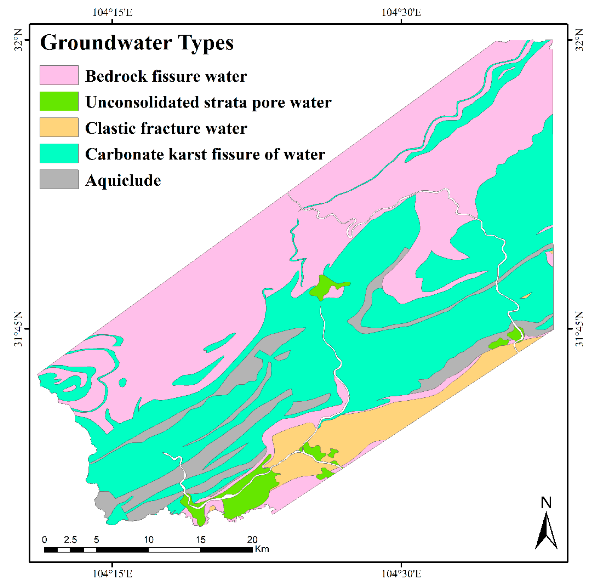
2.3.1. Data Description

Multi-source data were collected to establish the various factors required in the AHP technique, which included geological data, RS data, and hydrological data (

Table 3. Factors and data sources for groundwater potential assessment.

Category	Factor	Source Data	Data Precision
Geology	Rock	Geological Map	1:200,000
	Fault density
Topography	Slope	ASTER-GDEM V2	30 m
	Drainage density
	Convergence index
Hydrology	Rainfall	GSMaP	0.1° × 0.1°
	Distance from rivers	Open Street Map
Indicators	Enhanced vegetation index	Moderate-resolution Imaging Spectroradiometer	250 m
	Spring index	Hydrogeological Map	1:200,000

). The sources of geological data were the digital geological map provided by the National Geological Archives of China [56] and the digital hydrogeological map provided by the Geological Environment Monitoring Institute of China Geological Survey [48]. The geological data provide the geological background of the study area from a field survey, including rock, faults, distribution and flow rate of springs, and distribution of groundwater types. Such geological data are important to support this study of groundwater storage and movement. RS data sources were ASTER-GDEM V2 [57] and moderate-resolution imaging spectroradiometer (MODIS) [58], including the digital elevation model (DEM) and vegetation indices. The RS data can accurately reflect the surface indicators of groundwater and topographic features of the study area related to the convergence and divergence of groundwater. The hydrological data sources were the GSMaP satellite rainfall database and Open Street Map (OSM) dataset, from which the data of rainfall and rivers can be obtained. The GSMaP is a database of high-resolution global precipitation data developed by the Japan Aerospace Agency [59]. OSM comprises data recorded by volunteers worldwide and is updated in real-time [60]. Groundwater recharge in the study area can be reflected by rainfall and rivers in these hydrological data. The spatial database of the present study was reproduced using ArcGIS software with SAGA-GIS.

The above different types of data were used to establish groundwater potential assessment factors. Based on expert opinions and the previous literature, the selection of factors needs to be based on the purpose of the study and the characteristics of the study area [50]. Topographic, geological, and hydrological factors and groundwater indicators are commonly used to assess groundwater potential [50,51,52,61,62,63,64]. The topographic factors selected are slope, drainage density, and convergence index, which can influence high surface runoff generation. Hydrological factors selected from the data are rainfall and distance from rivers, which have important contributions to groundwater recharge. The EVI can be an effective indicator of groundwater in varied topographic areas. For the requirements of emergency water supply in varied topographic areas and the complex geological background of the study area, not only are the rock and fault density selected, but the direct spring index was established based on the distribution and flow rates of springs. The spring index provides a visual representation of the groundwater conditions in the study area. In a word, the occurrences and mobility of groundwater are explicitly or implicitly determined/revealed by these factors, as described in

Table 4. Description of groundwater potential assessment factors.

Factor	Description	Characteristics
Rock	Geological formations	Regional strata affect the porosity and permeability of aquifers.
Fault density	Line density of faults	The faults are conducive to the infiltration of groundwater.
Slope	The degree of steepness of the surface unit	The infiltration of surface water is inversely correlated with the slope.
Drainage density	The channel length per unit area	Seepage from surface water channels facilitates groundwater recharge.
Convergence index	The concavity or convexity of the landscape at a smaller spatial scale.	A negative convergence refers to concavities (e.g., valleys), whereas positive values reflect convex features (e.g., ridges).
Rainfall	Annual rainfall	Rainfall is an important source of groundwater recharge.
Distance from rivers	The distance of each grid to the nearest river	Aquifers close to rivers exhibit high recharge rates.
Enhanced vegetation index	Measurements of surface vegetation condition	Vegetation is a surface indicator of groundwater in varied topographic areas.
Spring index	Index calculated from actual spring locations and flow rates	The spring index provides a visual representation of the groundwater conditions in the study area.

and below.

Slope is a key factor in groundwater recharge. The infiltration of surface water is inversely correlated with slope. The slope determines surface water’s ability to either remain on the surface long enough to infiltrate into the ground or continue to flow [61]. The steep slopes result in a high water velocity and rapid runoff, which in turn increase erosion rates [52,65]. Thus, steep slopes yield poor groundwater recharge. The slope was derived from ASTER-GDEM V2 data with a spatial resolution of 30 m [57].

Other than the slope, many other factors are related to topography, such as curvature, convexity, etc. [29,64]. Considering the problem of multicollinearity, only the convergence index was used together with the slope. The convergence index reflects the concavity or convexity of a landscape at a smaller spatial scale, and it indicates the extent to which adjacent cells point to the center cell. A negative convergence refers to concavities (e.g., valleys), whereas positive values reflect convex features (e.g., ridges) [66,67]. The convergence index was calculated using SAGA-GIS software from ASTER-GDEM V2 data [57,68].

Rivers are important for groundwater recharge in varied topographic areas. Aquifers close to rivers exhibit high recharge rates [66]. As the distance from rivers increases, the probability of groundwater occurrence decreases [69,70]. The data of rivers were obtained from the OSM dataset, and the distance from rivers was generated using the “Euclidean distance function” in ArcGIS. Furthermore, the drainage density of surface water channels was used, as seepage from channels facilitates groundwater recharge [34,51]. Drainage density represents the channel length per unit area and is calculated using [71]:

$${\mathrm{D}}_{\mathrm{d}}{=\mathrm{L}/\mathrm{A}}_{\mathrm{d}}$$

(9)

where L is the length of channels, and ${\mathrm{A}}_{\mathrm{d}}$ is the area of the drainage basin. A high channel density yields high groundwater potential. The surface water channels were extracted from ASTER-GDEM V2 data in SAGA-GIS based on the flow and flow direction [57,68], and this factor was prepared using the line density analysis tool in ArcGIS.

Aquifers are usually recharged by effective rainfall. The rate and distribution of rainfall significantly influence hydrogeological conditions [62]. High rainfall is associated with increased groundwater potential. Rainfall data of the study area for 2020, with a resolution of $0.1°\times 0.1°$, were collected from the GSMaP satellite rainfall database [59].

The area is on the Longmenshan Fault, which significantly influences groundwater. Faults result in notable secondary porosity and permeability, providing a pathway for groundwater to flow into the subsurface [46]. The high fault density in varied topographic areas is favorable for groundwater potential. The data of faults were extracted from the China National Digital Geological Map (Public Version at 1:200,000 Scale) Spatial Database [56]. The fault density was calculated using the line density analysis tool in ArcGIS.

Vegetation is a proper surface indicator of groundwater in varied topographic areas [33]. Compared with other vegetation indices such as the NDVI, EVI enhances the vegetation signal and can accurately characterize the spatial and temporal information of vegetation in areas with high vegetation cover [72]. The EVI dataset was collected from the MODIS product named MOD13Q1, which has a spatial resolution of 250 m [58]. The EVI was obtained for April when vegetation growth is abundant.

Geological formations affect the porosity and permeability of aquifers and play a pivotal role in groundwater recharge and occurrence [50,73]. Thus, regional rock is considered a key factor affecting groundwater recharge, quantity, and quality [73]. The data of rock were also extracted from the China National Digital Geological Map (Public Version at 1:200,000 Scale) Spatial Database [56].

The distribution and flow rate of springs are often used to accurately gauge groundwater. For reasonable assessment in this area with a complex geological background, the location and flow rate of actual springs are assimilated to form the spring index. A high spring index indicates high groundwater potential. The distribution and flow rate of springs were extracted from the hydrogeological map provided by the Geological Environment Monitoring Institute of China Geological Survey [48]. The spring index was created through the following four steps: (1) using the “Euclidean distance function” in ArcGIS to calculate the distance from each pixel to the nearest spring; (2) normalizing the distance to the nearest spring, with low weights for long distances and high weights for short ones; (3) using the “Euclidean allocation function” in ArcGIS to assign each pixel to the flow rate of the nearest spring; and (4) multiplying the normalized distance by the logarithm of the flow rate at each pixel to obtain the spring index as:

$$\mathrm{Spring}\mathrm{index}=\mathrm{D}\times \lg \left(\mathrm{F}\right)$$

(10)

where D is the normalized distance to the nearest spring, and F is the flow rate of the nearest spring. Due to the wide range of flow rate values, the logarithm of the spring flow rate was applied.

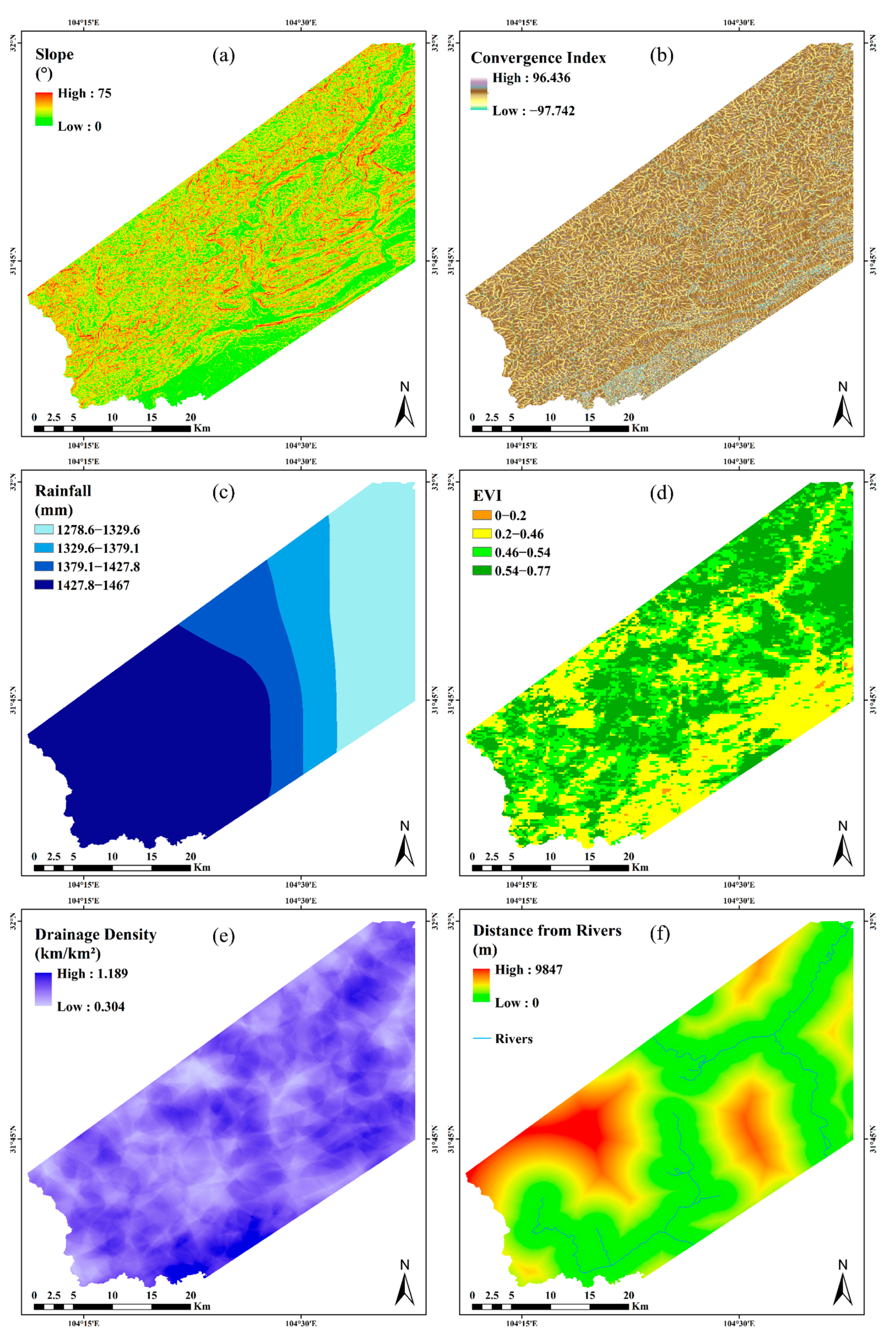
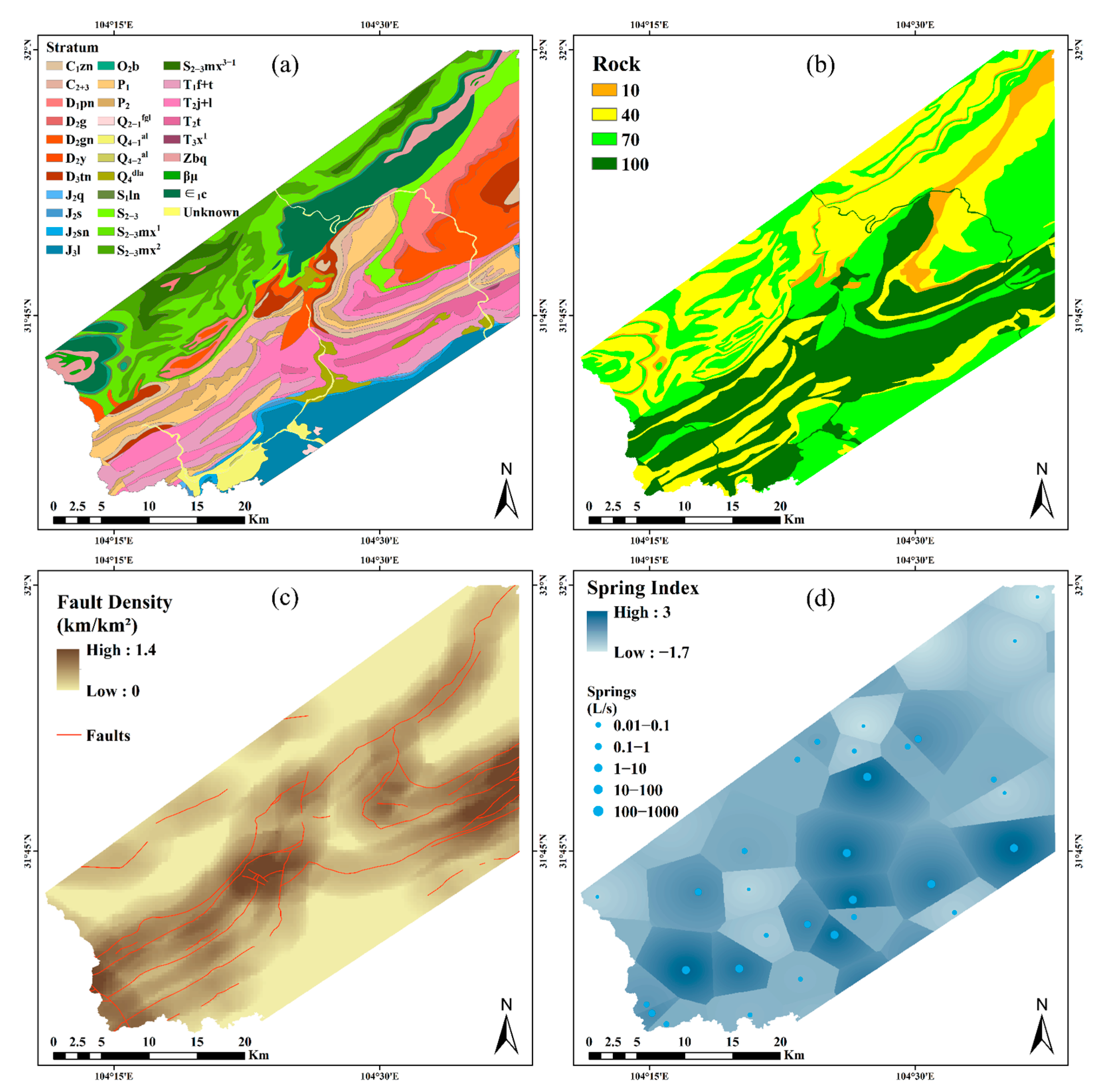
2.3.2. Factor Analysis

The nine factors were integrated using ArcGIS software. Each dataset was converted into a grid format with 30 m spatial resolution for use in the groundwater inventory of the study area (Figure 4 and Figure 5).

The slope ranges from 0$°$ to 75$°$. Most of the areas have slopes of less than 20$°$ (gentle slope), and the slopes in the varied topographic areas are mainly less than 50$°$. Steep slopes were assigned low weights when normalized. The convergence index ranges between −97.742 and 96.436. Negative values were assigned high weights at normalization.

Annual rainfall was mapped using the ordinary kriging interpolation technique in ArcGIS. Rainfall in this area tends to be high in the west and low in the east. The maximum annual rainfall is 1467 mm, and the range of rainfall spans 188 mm.

The EVI values range from 0.14 to 0.77 in this area. An EVI higher than 0.2 represents vegetation, and the higher the EVI value, the denser the vegetation. High EVI values were assigned high weights at normalization.

The drainage density ranges from 0.304 ${\mathrm{km}/\mathrm{km}}^2$ to 1.189 ${\mathrm{km}/\mathrm{km}}^2$. The high drainage density occurs near perennial streams (Tongkou, Anchang, and Subao Rivers) and was assigned a high weight when normalized. Furthermore, the farthest distance is 9847 m, and the average distance is 2865 m in the area. The close distances were assigned high weights at normalization.

The rocks were divided into four classes and assigned weights (10, 40, 70, 100), with a high weight (100) representing high groundwater potential and a low weight (10) representing low groundwater potential. A part of the high-weight area (100) comprises young alluvium, most of which are riverbed and flood plain gravel alluvium, as well as some slope alluvium. Another part of the high-weight area consists of Middle Triassic strata and Permian strata, which are mainly composed of limestone, shale, and dolomite, and karst groundwater is highly developed. The low-weight area (10) includes Jurassic Middle strata and Silurian strata, which have limited infiltration and groundwater recharge capacity.

The values of fault density range from 0 to 1.39 ${\mathrm{km}/\mathrm{km}}^2$. The high fault density was assigned a high weight when normalized. Moreover, the spring index varies from −1.7 to 3. High spring index values are mainly observed in the southwest and east, whereas the values are low in the northeast.

3. Results

3.1. Multicollinear Analysis

The multicollinear analysis results are shown in

Table 5. Collinearity assessment results for the factors.

	Factor	Tolerance	VIF		Factor	Tolerance	VIF
1	Rock	0.816	1.225	6	EVI	0.805	1.242
2	Fault density	0.936	1.068	7	Convergence index	0.984	1.016
3	Spring index	0.739	1.353	8	Rainfall	0.871	1.148
4	Slope	0.909	1.100	9	Distance from rivers	0.783	1.277
5	Drainage density	0.782	1.279

. The results demonstrate VIF values less than 10 and tolerance values exceeding 0.1 for each factor ($\mathsf{\rho }<0.01$ and $<0.05$, respectively), indicating no collinearity among the nine factors used in this study; therefore, there was no significant uncertainty in the model results.

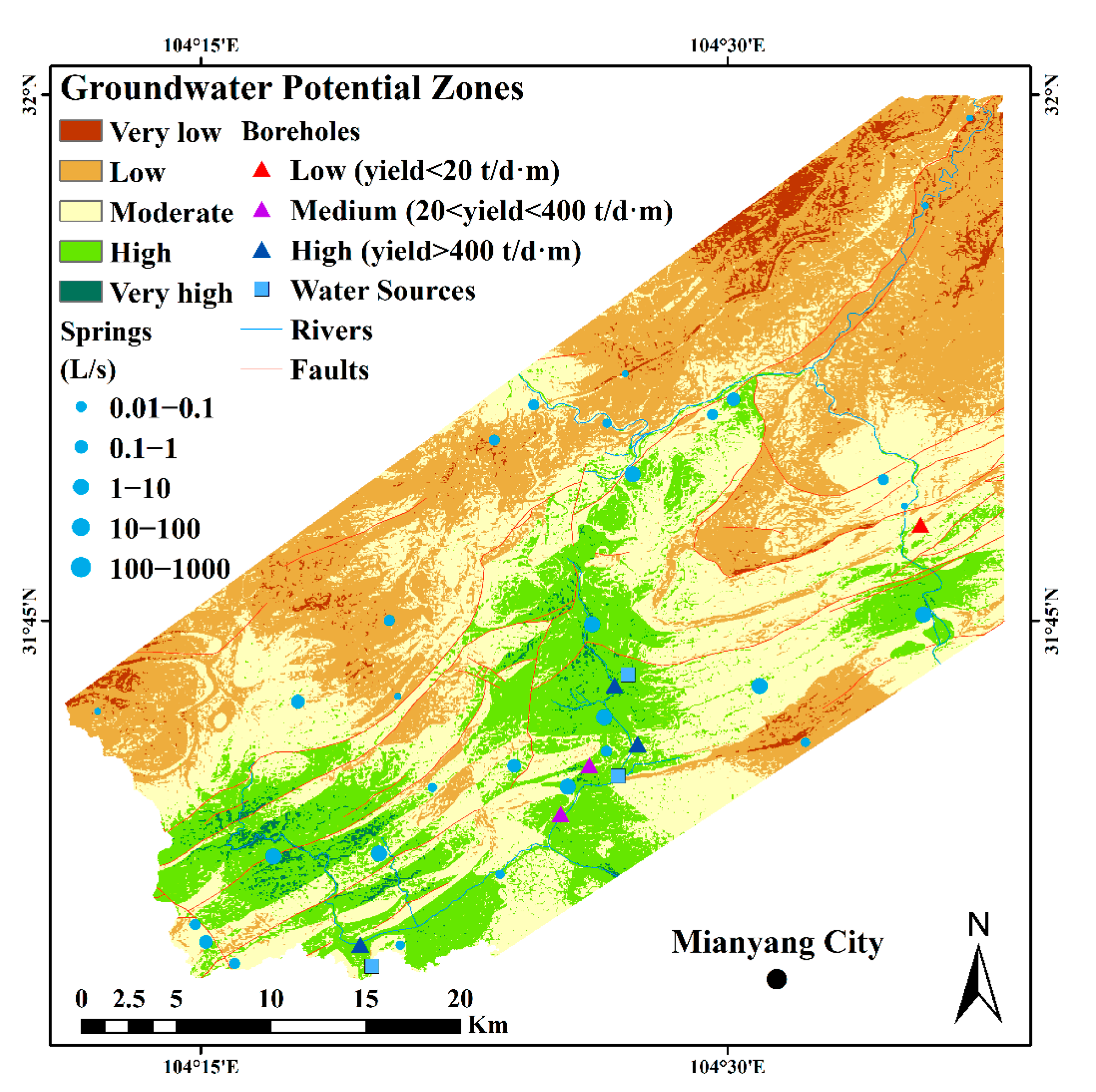
3.2. Groundwater Potential Map

The CR of the factors was calculated before overlay analysis (

Table 6. Pairwise comparison matrix for the factors and consistency validation.

	Rock	SL	CI	SI	FD	DD	DR	RAIN	EVI	Priority	${\mathit{\lambda }}_{\mathit{m}\mathit{a}\mathit{x}}$	CI	CR
Rock	1	1	9/8	9/8	9/7	9/6	9/6	9/5	9/4	0.145	9	0	0
SL	1	1	9/8	9/8	9/7	9/6	9/6	9/5	9/4	0.145
CI	8/9	8/9	1	1	8/7	8/6	8/6	8/5	8/4	0.129
SI	8/9	8/9	1	1	8/7	8/6	8/6	8/5	8/4	0.129
FD	7/9	7/9	7/8	7/8	1	7/6	7/6	7/5	7/4	0.113
DD	6/9	6/9	6/8	6/8	6/7	1	1	6/5	6/4	0.097
DR	6/9	6/9	6/8	6/8	6/7	1	1	6/5	6/4	0.097
RAIN	5/9	5/9	5/8	5/8	5/7	5/6	5/6	1	5/4	0.081
EVI	4/9	4/9	4/8	4/8	4/7	4/6	4/6	4/5	1	0.065
Sum	6.889	6.889	7.75	7.75	8.857	10.333	10.333	12.4	15.5

SL: slope; CI: convergence index; CR: consistency ratio; SI: spring index; FD: fault density: DD: drainage density; DR: distance from rivers; RAIN: rainfall.

). The CR value was less than 0.1, indicating that the judgment matrix was valid and consistent. The nine normalized factors were overlaid based on the obtained weights (Table 6), and the final GWP was created by overlay analysis (Equation (6)).

In this varied topographic area, we find the geological conditions that are most important for groundwater potential estimation. This area was divided into five categories (very low, low, moderate, high, and very high groundwater potential zones) using the grading method with equal intervals (Figure 6). This was attributed as 0.26–0.37 (very low), 0.37–0.48 (low), 0.48–0.6 (moderate), 0.6–0.71 (high), and 0.71–0.82 (very high). The data of six boreholes and three water supply sources were collected from the Geological Environment Monitoring Institute of China Geological Survey to validate the GWP. The borehole data include the yield rate and the drawdown, which was converted into the yield rate per unit drawdown for convenient comparison. Water supply sources are divided into three levels according to the water supply capacity, namely level 1 (500–5000 t/d), level 2 (5000–20,000 t/d), level 3 (>20,000 t/d). The results of the comparison are shown in

Table 7. Comparison of borehole yield rate, water source level, and groundwater potential values.

Yield (t/d·m)	GWP	Potentiality	Water Source Level	GWP	Potentiality
2	0.48	Low	2	0.62	High
41.8	0.58	Moderate	3	0.69	High
148.3	0.59	Moderate	3	0.73	Very high
468.6	0.63	High
1464.4	0.64	High
2541.9	0.69	High

. A correlation analysis between GWP and spring flow rates was performed, where the logarithm of the spring flow rate was applied due to the wide range of flow rate values (Figure 7). The GWP in the study area is positively correlated with the flow rates of springs, while the distribution and flow rates of springs correspond well with the groundwater potential zones (Figure 6 and Figure 7). The borehole yield rate exhibits a strong exponential relationship with the GWP (Figure 7). The ${\mathrm{R}}^2$ is 0.917 and the RMSE is 329.03 $\mathrm{t}/\mathrm{d}·\mathrm{m}$, implying that GWP is a reasonable predictor of the actual groundwater potential, but it is still biased by the outliers. The groundwater potential zones approximately correspond to the yield rates as very low ($<1\mathrm{t}/\mathrm{d}·\mathrm{m}$), low (1–20$\mathrm{t}/\mathrm{d}·\mathrm{m}$), moderate (20–400 $\mathrm{t}/\mathrm{d}·\mathrm{m}$), high (400–4000 $\mathrm{t}/\mathrm{d}·\mathrm{m}$), or very high ($>4000\mathrm{t}/\mathrm{d}·\mathrm{m}$).

Water sources can only roughly reflect groundwater potential because the selection usually involves the consideration of surface water and groundwater. The area contains one level 2 water source and one level 3 water source located in high groundwater potential zones, and another level 3 water source situated in a very high groundwater potential zone. The comparison suggests that the GWP has a positive correlation with the water source level.

4. Discussion

Among the factors for evaluating groundwater potential in varied topographic areas, geological and topographic factors (e.g., rock, slope) are often assigned high weights, whereas factors for groundwater recharge and faults (e.g., fault density, rainfall) are assigned either high or low weights depending on regional conditions [46,61,62]. Based on Table 6, rock, slope, and convergence index are assigned high weights, whereas fault density is assigned a high weight due to the Longmenshan Fault. The factors for groundwater recharge are given a relatively low weight because of the sparse rivers and insufficient accuracy of rainfall data. The spring index and EVI are indicators of groundwater for complex geological backgrounds. The spring index can effectively reflect the groundwater condition and is assigned a high weight. In general, geological factors (rock, fault density) and topographic factors (slope, convergence index) are more dominant in varied topographic areas than in flat areas in relation to the assessment of groundwater potential.

Based on the results, approximately 2.66% and 0.75% of the area exhibits yield rates of $<1\mathrm{t}/\mathrm{d}·\mathrm{m}$ and $>4000\mathrm{t}/\mathrm{d}·\mathrm{m}$, respectively. In addition, approximately 36.1%, 39.62%, and 20.88% of the area are identified as yield rates of 1–20 $\mathrm{t}/\mathrm{d}·\mathrm{m}$, 20–400 $\mathrm{t}/\mathrm{d}·\mathrm{m}$, and 400–4000 $\mathrm{t}/\mathrm{d}·\mathrm{m}$, respectively.

Compared with the groundwater types (Figure 3), the map of GWP shows a more detailed distribution of groundwater. GWP in bedrock fissure water areas tends to be low, and it can even be very low with yield rates $<1\mathrm{t}/\mathrm{d}·\mathrm{m}$ in areas with very high elevation. Bedrock areas are not recommended for centralized water supply due to limited transportation. Clastic fracture water areas are located in the piedmont zone with low terrain, where have mostly moderate groundwater potential, and even high groundwater potential in areas close to rivers. Although these areas are indeed easy to exploit, the spring index indicates that there are still zones with low and very low groundwater potential and the yield rates $<20\mathrm{t}/\mathrm{d}·\mathrm{m}$ in the areas with uplifted terrain (high slopes, positive convergence index). The unconsolidated strata pore water is distributed in the alluvium with a water-rich loose structure. These areas are ideal groundwater exploitation sites, corresponding to high yield rates. The areas with carbonate karst fissure of water are distributed along the faults that have above moderate groundwater potential and are suitable groundwater exploitation sites in varied topographic areas. Around the aquiclude, the map exhibits a staggered distribution of high and very high groundwater potential zones mixed with moderate and low groundwater potential zones due to water-blocking faults. These water-blocking faults separate the aquifer and the aquiclude, thus enriching the karst groundwater in the aquifer; however, the carbonate and clastic rocks are interbedded in the aquiclude, without the karst being well developed. Due to this property of water-blocking faults, the aquiclude can be an important indicator for finding karst aquifers despite its low groundwater potential.

The groundwater recharge in the study area originates from both rainfall and surface water. Correspondingly, the western area, exhibiting notably higher rainfall, has more zones with high and very high groundwater potential than the eastern area. Furthermore, high and very high groundwater potential zones are concentrated in the vicinity of Anchang River, Subao River, and Tongkou River in the southeast. These zones are situated in valleys with low slopes and concave topography, which promote groundwater convergence. The valleys adjacent to these rivers are often river floodplains and terraces with water-rich loose aquifers. In addition, faults strongly influence groundwater in varied topographic areas. Substantial karst groundwater with very high groundwater potential develops along the faults. The properties of faults also affect groundwater distribution, as the aquifers vary markedly in groundwater potential when a water-blocking fault is developed.

The results show that the integration of a moderate amount of multi-source data using the AHP method can reasonably assess varied topographic areas with complex geological backgrounds. The flexibility of this method allows us to modify the weights of the factors and their logical nature is generic, so we can apply the same method in other regions with suitable modifications. The method may be used for varied topographic areas with similar geological backgrounds, in which geological and topographic factors may be dominant and factors established on high-precision hydrological data may be assigned high weights. However, the method still has some limitations. The AHP is a knowledge-driven process and therefore may inhibit some errors in its prediction [52]. Furthermore, the nine factors are still inadequate for groundwater evaluation, despite the assimilation of the spring index. Some factors not adopted by the study, such as LULC, aquifer thickness, depth to groundwater, hydraulic conductivity, and soil type, all have important effects on groundwater potential. In addition, the accuracy of the rainfall data used in the study was not high. In the future, the GWP can be improved using more high-precision data and considering all these factors.

5. Conclusions

In this study, a GIS-based method using AHP was adopted to identify groundwater potential zones in the central varied topographic area of Mianyang City. Topographic factors (slope, convergence index, and drainage density), geological factors (rock and fault density), groundwater recharge factors (rainfall and distance from rivers), and EVI were established based on the previous literature. Considering the complex geographical background of the study area, the spring index was established by assimilating the spring data, the addition of which effectively increased the accuracy of the GWP. These factors were integrated to provide a reasonable groundwater potential assessment based on multi-source data. The available borehole data and multicollinear checks were used to validate the effectiveness of the GWP. The results show that the GWP can reasonably reflect the distribution of groundwater to a certain extent. In this assessment, rock, slope, convergence index, and fault density are important groundwater potential factors, whereas the drainage density, distance from rivers, and rainfall are relatively minor factors. The flexibility of this method allows us to modify the weights of the factors, and their logical nature is generic; thus, the same method can be applied in other regions with suitable modifications. For groundwater assessment in areas with different geological conditions, factors related to geology and topography are always important; however, the weights of faults and groundwater recharge need to be adjusted according to regional conditions. The proposed approach may be referred to apply in most varied topographic areas with different geological backgrounds, whereas factors established based on high-precision hydrological data may be assigned high weights.

The results suggest approximately 20.88% and 0.75% of the area exhibit high and very high groundwater potential, maybe corresponding to the yield rates of 400–4000 $\mathrm{t}/\mathrm{d}·\mathrm{m}$ and $>4000\mathrm{t}/\mathrm{d}·\mathrm{m}$. The groundwater types in the high and very high groundwater potential zones mainly consist of unconsolidated strata pore water and carbonate karst fissure of water, both of which are ideal groundwater sources. The recommended sites for groundwater exploitation and emergency water supply are located in valleys and fracture areas near Anchang River, Subao River, and Tongkou River, where the fracture areas are ideal groundwater sources in varied topographic areas. For groundwater exploitation and emergency water supply needs in bedrock areas, places close to rivers and in depressed terrain may be appropriate. The results of this research contribute to the comprehensive management of groundwater exploration and the exploitation of groundwater sources, and can also provide an effective plan for emergency water supply. The approach in this study can be a reference for other areas requiring groundwater sources. Policymakers can effectively analyze the results of groundwater assessment for rational management.

References

1. Watto, M.A. The Economics of Groundwater Irrigation in the Indus Basin, Pakistan: Tube-Well Adoption, Technical and Ir-rigation Water Efficiency and Optimal Allocation. Ph.D. Thesis, University of Western Australia, Perth, Australia, 2015. [Google Scholar]
2. Oke, S.A.; Fourie, F. Guidelines to groundwater vulnerability mapping for Sub-Saharan Africa. Groundw. Sustain. Dev. 2017, 5, 168–177. [Google Scholar] [CrossRef]
3. Wang, Z.; Yi, F.C. AHP-based evaluation of occurrence easiness of geological disasters in Mianyang City. J. Nat. Disasters 2009, 18, 14–23. [Google Scholar] [CrossRef]
4. Vadiati, M.; Asghari-Moghaddam, A.; Nakhaei, M.; Adamowski, J.; Akbarzadeh, A. A fuzzy-logic based decision-making approach for identification of groundwater quality based on groundwater quality indices. J. Environ. Manag. 2016, 184, 255–270. [Google Scholar] [CrossRef]
5. Lan, Y.; Jin, M.; Yan, C.; Zou, Y. Schemes of groundwater exploitation for emergency water supply and their environmental impacts on Jiujiang City, China. Environ. Earth Sci. 2014, 73, 2365–2376. [Google Scholar] [CrossRef]
6. Naghibi, S.A.; Moghaddam, D.D.; Kalantar, B.; Pradhan, B.; Kisi, O. A comparative assessment of GIS-based data mining models and a novel ensemble model in groundwater well potential mapping. J. Hydrol. 2017, 548, 471–483. [Google Scholar] [CrossRef]
7. Sichuan Hydrology and Water Resources Survey Bureau. Water Resources Bulletin of Sichuan Province, China; Sichuan Provincial Water Resources Department: Sichuan, China, 2019. [Google Scholar]
8. Russoniello, C.J.; Michael, H.A.; Fernandez, C.; Andres, A.S.; He, C.; Madsen, J.A. Investigation of Submarine Groundwater Discharge at Holts Landing State Park, Delaware: Hydrogeologic Framework, Groundwater Level and Salinity Observations; Delaware Geological Survey, University of Delaware: Newark, DE, USA, 2017. [Google Scholar]
9. Helaly, A.S. Assessment of groundwater potentiality using geophysical techniques in Wadi Allaqi basin, Eastern Desert, Egypt—Case study. NRIAG J. Astron. Geophys. 2017, 6, 408–421. [Google Scholar] [CrossRef] [Green Version]
10. Moss, R.; Moss, G.E. Handbook of Ground Water Development; Wiley-Interscience: New York, NY, USA, 1990. [Google Scholar]
11. Patra, S.; Mishra, P.; Mahapatra, S.C. Delineation of groundwater potential zone for sustainable development: A case study from Ganga Alluvial Plain covering Hooghly district of India using remote sensing, geographic information system and analytic hierarchy process. J. Clean. Prod. 2018, 172, 2485–2502. [Google Scholar] [CrossRef]
12. Nampak, H.; Pradhan, B.; Manap, M.A. Application of GIS based data driven evidential belief function model to predict groundwater potential zonation. J. Hydrol. 2014, 513, 283–300. [Google Scholar] [CrossRef]
13. Lee, S.; Lee, C.-W.; Kim, J.-C. Groundwater productivity potential mapping using logistic regression and boosted tree models: The case of Okcheon City in Korea. Arab. J. Geosci. 2019, 305–307. [Google Scholar] [CrossRef]
14. Park, S.-H.; Jung, H.-S.; Choi, J.; Jeon, S. A quantitative method to evaluate the performance of topographic correction models used to improve land cover identification. Adv. Space Res. 2017, 60, 1488–1503. [Google Scholar] [CrossRef]
15. Baek, W.-K.; Jung, H.-S.; Jo, M.-J.; Lee, W.-J.; Zhang, L. Ground subsidence observation of solid waste landfill park using multi-temporal radar interferometry. Int. J. Urban Sci. 2019, 23, 406–421. [Google Scholar] [CrossRef]
16. Kim, J.-C.; Kim, D.-H.; Park, S.-H.; Jung, H.-S.; Shin, H.-S. Application of Landsat images to Snow Cover Changes by volcanic activities at Mt. Villarrica and Mt. Llaima, Chile. Korean J. Remote. Sens. 2014, 30, 341–350. [Google Scholar] [CrossRef] [Green Version]
17. Tweed, S.O.; Leblanc, M.; Webb, J.; Lubczynski, M.W. Remote sensing and GIS for mapping groundwater recharge and discharge areas in salinity prone catchments, southeastern Australia. Hydrogeol. J. 2006, 15, 75–96. [Google Scholar] [CrossRef]
18. Aluko, O.E.; Igwe, O. An integrated geomatics approach to groundwater potential delineation in the Akoko-Edo Area, Nigeria. Environ. Earth Sci. 2017, 76, 240. [Google Scholar] [CrossRef]
19. Goodchild, M.F. Geographic information systems. In Encyclopedia of Theoretical Ecology; University of California Press: Oakland, CA, USA, 2012; pp. 341–345. [Google Scholar] [CrossRef]
20. Elfadaly, A.; Attia, W.; Lasaponara, R. Monitoring the environmental risks around Medinet Habu and Ramesseum Temple at West Luxor, Egypt, using remote sensing and GIS techniques. J. Archaeol. Method Theory 2017, 25, 587–610. [Google Scholar] [CrossRef]
21. Elmahdy, S.I.; Mohamed, M.M. Automatic detection of near surface geological and hydrological features and investigating their influence on groundwater accumulation and salinity in southwest Egypt using remote sensing and GIS. Geocarto Int. 2014, 30, 1–13. [Google Scholar] [CrossRef]
22. Das, N.; Mukhopadhyay, S. Application of multi-criteria decision making technique for the assessment of groundwater potential zones: A study on Birbhum district, West Bengal, India. Environ. Dev. Sustain. 2018, 22, 931–955. [Google Scholar] [CrossRef]
23. Anbarasu, S.; Brindha, K.; Elango, L. Multi-influencing factor method for delineation of groundwater potential zones using remote sensing and GIS techniques in the western part of Perambalur district, southern India. Earth Sci. Inform. 2019, 13, 317–332. [Google Scholar] [CrossRef]
24. Lee, S.; Hyun, Y.; Lee, M.-J. Groundwater potential mapping using data mining models of big data analysis in Goyang-si, South Korea. Sustainability 2019, 11, 1678. [Google Scholar] [CrossRef] [Green Version]
25. Al-Abadi, A.M. Modeling of groundwater productivity in northeastern Wasit Governorate, Iraq using frequency ratio and Shannon’s entropy models. Appl. Water Sci. 2017, 7, 699–716. [Google Scholar] [CrossRef] [Green Version]
26. Rahmati, O.; Pourghasemi, H.R.; Melesse, A.M. Application of GIS-based data driven random forest and maximum entropy models for groundwater potential mapping: A case study at Mehran Region, Iran. Catena 2016, 137, 360–372. [Google Scholar] [CrossRef]
27. Golkarian, A.; Naghibi, S.A.; Kalantar, B.; Pradhan, B. Groundwater potential mapping using C5.0, random forest, and multivariate adaptive regression spline models in GIS. Environ. Monit. Assess. 2018, 190, 149. [Google Scholar] [CrossRef] [PubMed]
28. Park, S.; Hamm, S.-Y.; Jeon, H.-T.; Kim, J. Evaluation of logistic regression and multivariate adaptive regression spline models for groundwater potential mapping using R and GIS. Sustainability 2017, 9, 1157. [Google Scholar] [CrossRef] [Green Version]
29. Kim, J.-C.; Jung, H.-S.; Lee, S. Spatial mapping of the groundwater potential of the geum river basin using ensemble models based on remote sensing images. Remote Sens. 2019, 11, 2285. [Google Scholar] [CrossRef] [Green Version]
30. Panahi, M.; Sadhasivam, N.; Pourghasemi, H.R.; Rezaie, F.; Lee, S. Spatial prediction of groundwater potential mapping based on convolutional neural network (CNN) and support vector regression (SVR). J. Hydrol. 2020, 588, 125033. [Google Scholar] [CrossRef]
31. Pradhan, A.M.S.; Kim, Y.-T.; Shrestha, S.; Huynh, T.-C.; Nguyen, B.-P. Application of deep neural network to capture groundwater potential zone in mountainous terrain, Nepal Himalaya. Environ. Sci. Pollut. Res. 2021, 28, 18501–18517. [Google Scholar] [CrossRef] [PubMed]
32. Kord, M.; Moghaddam, A.A. Spatial analysis of Ardabil plain aquifer potable groundwater using fuzzy logic. J. King Saud Univ. Sci. 2014, 26, 129–140. [Google Scholar] [CrossRef] [Green Version]
33. Aouragh, M.H.; Essahlaoui, A.; El Ouali, A.; El Hmaidi, A.; Kamel, S. Groundwater potential of Middle Atlas plateaus, Morocco, using fuzzy logic approach, GIS and remote sensing. Geomat. Nat. Hazards Risk 2017, 8, 194–206. [Google Scholar] [CrossRef] [Green Version]
34. Das, S. Comparison among influencing factor, frequency ratio, and analytical hierarchy process techniques for groundwater potential zonation in Vaitarna basin, Maharashtra, India. Groundw. Sustain. Dev. 2019, 8, 617–629. [Google Scholar] [CrossRef]
35. Quan, H.-C.; Lee, B.-G. GIS-based landslide susceptibility mapping using analytic hierarchy process and artificial neural network in Jeju (Korea). KSCE J. Civ. Eng. 2012, 16, 1258–1266. [Google Scholar] [CrossRef]
36. Lu, Z.; Deng, Z.; Wang, D.; Zhao, H.; Wang, G.; Xu, H. Overview of the research progress of groundwater resources assessment technology based on remote sensing. Geol. Surv. China 2021, 114–124. [Google Scholar] [CrossRef]
37. Saaty, T.L. Decision making—The analytic hierarchy and network processes (AHP/ANP). J. Syst. Sci. Syst. Eng. 2004, 13, 1–35. [Google Scholar] [CrossRef]
38. Brunelli, M. Introduction to the Analytic Hierarchy Process; Springer: Singapore, 2015. [Google Scholar]
39. Saaty, R. The analytic hierarchy process—What it is and how it is used. Math. Model. 1987, 9, 161–176. [Google Scholar] [CrossRef] [Green Version]
40. Mu, E.; Pereyra-Rojas, M. Understanding the analytic hierarchy process. In Practical Decision Making; Springer: Cham, Switzerland, 2017; pp. 7–22. [Google Scholar] [CrossRef]
41. Murmu, P.; Kumar, M.; Lal, D.; Sonker, I.; Singh, S.K. Delineation of groundwater potential zones using geospatial techniques and analytical hierarchy process in Dumka district, Jharkhand, India. Groundw. Sustain. Dev. 2019, 9, 100239. [Google Scholar] [CrossRef]
42. Kumar, V.A.; Mondal, N.C.; Ahmed, S. Identification of groundwater potential zones using RS, GIS and AHP techniques: A case study in a part of Deccan Volcanic Province (DVP), Maharashtra, India. J. Indian Soc. Remote Sens. 2020, 48, 497–511. [Google Scholar] [CrossRef]
43. Andualem, T.G.; Demeke, G.G. Groundwater potential assessment using GIS and remote sensing: A case study of Guna tana landscape, upper blue Nile Basin, Ethiopia. J. Hydrol. Reg. Stud. 2019, 24, 100610. [Google Scholar] [CrossRef]
44. Dar, T.; Rai, N.; Bhat, A. Delineation of potential groundwater recharge zones using analytical hierarchy process (AHP). Geol. Ecol. Landsc. 2020, 1–16. [Google Scholar] [CrossRef] [Green Version]
45. Lee, S.; Song, K.-Y.; Kim, Y.; Park, I. Regional groundwater productivity potential mapping using a geographic information system (GIS) based artificial neural network model. Hydrogeol. J. 2012, 20, 1511–1527. [Google Scholar] [CrossRef]
46. Pinto, D.; Shrestha, S.; Babel, M.S.; Ninsawat, S. Delineation of groundwater potential zones in the Comoro watershed, Timor Leste using GIS, remote sensing and analytic hierarchy process (AHP) technique. Appl. Water Sci. 2017, 7, 503–519. [Google Scholar] [CrossRef] [Green Version]
47. Yang, Y.; Zhang, X.; Hua, Q.; Su, L.; Feng, C.; Qiu, Y.; Liang, C.; Su, J.; Gu, Y.; Jin, Z. Segmentation characteristics of the Longmenshan fault—Constrained from dense focal mechanism data. Chin. J. Geophys. 2021, 64, 1181–1205. [Google Scholar]
48. Mu, H.; Chen, H.; Zhang, Z.; Zhang, B. China national digital hydrogeological map (At 1:200,000 Scale) spatial database. Geol. China 2021, 48, 124–138. [Google Scholar] [CrossRef]
49. Ishizaka, A.; Nemery, P. Multi-Criteria Decision Analysis: Methods and Software; Wiley: Hoboken, NJ, USA, 2013. [Google Scholar]
50. Kaur, L.; Rishi, M.S.; Singh, G.; Thakur, S.N. Groundwater potential assessment of an alluvial aquifer in Yamuna sub-basin (Panipat region) using remote sensing and GIS techniques in conjunction with analytical hierarchy process (AHP) and catastrophe theory (CT). Ecol. Indic. 2020, 110, 105850. [Google Scholar] [CrossRef]
51. Arshad, A.; Zhang, Z.; Zhang, W.; Dilawar, A. Mapping favorable groundwater potential recharge zones using a GIS-based analytical hierarchical process and probability frequency ratio model: A case study from an agro-urban region of Pakistan. Geosci. Front. 2020, 11, 1805–1819. [Google Scholar] [CrossRef]
52. Mukherjee, I.; Singh, U. Delineation of groundwater potential zones in a drought-prone semi-arid region of east India using GIS and analytical hierarchical process techniques. Catena 2020, 194, 104681. [Google Scholar] [CrossRef]
53. Saha, S. Groundwater potential mapping using analytical hierarchical process: A study on Md. Bazar Block of Birbhum District, West Bengal. Spat. Inf. Res. 2017, 25, 615–626. [Google Scholar] [CrossRef]
54. Tamura, R.; Kobayashi, K.; Takano, Y.; Miyashiro, R.; Nakata, K.; Matsui, T. Mixed integer quadratic optimization formulations for eliminating multicollinearity based on variance inflation factor. J. Glob. Optim. 2018, 73, 431–446. [Google Scholar] [CrossRef]
55. Dormann, C.F.; Elith, J.; Bacher, S.; Buchmann, C.; Carl, G.; Carré, G.; Marquéz, J.R.G.; Gruber, B.; Lafourcade, B.; Leitão, P.J.; et al. Collinearity: A review of methods to deal with it and a simulation study evaluating their performance. Ecography 2013, 36, 27–46. [Google Scholar] [CrossRef]
56. Li, C.; Wang, X.; He, C.; Wu, X.; Kong, Z.; Li, X. China national digital geological map (Public Version at 1:200,000 Scale) spatial database. Geol. China 2019, 46, 1–10. [Google Scholar] [CrossRef]
57. Geospatial Data Cloud. Available online: www.gscloud.cn (accessed on 3 March 2021).
58. Earthdata. Available online: Search.earthdata.nasa.gov/search (accessed on 3 March 2021).
59. GSMaP Global Satellite Mapping of Precipitation. Available online: Sharaku.eorc.jaxa.jp/GSMaP/index.htm (accessed on 6 May 2021).
60. OpenStreetMap. Available online: Download.geofabrik.de (accessed on 3 May 2021).
61. Oikonomidis, D.; Dimogianni, S.; Kazakis, N.; Voudouris, K. A GIS/Remote Sensing-based methodology for groundwater potentiality assessment in Tirnavos area, Greece. J. Hydrol. 2015, 525, 197–208. [Google Scholar] [CrossRef]
62. Shao, Z.; Huq, E.; Cai, B.; Altan, O.; Li, Y. Integrated remote sensing and GIS approach using Fuzzy-AHP to delineate and identify groundwater potential zones in semi-arid Shanxi Province, China. Environ. Model. Softw. 2020, 134, 104868. [Google Scholar] [CrossRef]
63. Serele, C.; Pérez-Hoyos, A.; Kayitakire, F. Mapping of groundwater potential zones in the drought-prone areas of south Madagascar using geospatial techniques. Geosci. Front. 2020, 11, 1403–1413. [Google Scholar] [CrossRef]
64. Lee, S.; Hyun, Y.; Lee, S.; Lee, M.-J. Groundwater potential mapping using remote sensing and GIS-based machine learning techniques. Remote Sens. 2020, 12, 1200. [Google Scholar] [CrossRef] [Green Version]
65. Yang, J.; Zhang, H.; Ren, C.; Nan, Z.; Wei, X.; Li, C. A cross-reconstruction method for step-changed runoff series to implement frequency analysis under changing environment. Int. J. Environ. Res. Public Health 2019, 16, 4345. [Google Scholar] [CrossRef] [Green Version]
66. Naghibi, S.A.; Hashemi, H.; Berndtsson, R.; Lee, S. Application of extreme gradient boosting and parallel random forest algorithms for assessing groundwater spring potential using DEM-derived factors. J. Hydrol. 2020, 589, 125197. [Google Scholar] [CrossRef]
67. Conoscenti, C.; Ciaccio, M.; Caraballo-Arias, N.A.; Gómez-Gutiérrez, A.; Rotigliano, E.; Agnesi, V. Assessment of susceptibility to earth-flow landslide using logistic regression and multivariate adaptive regression splines: A case of the Belice River basin (western Sicily, Italy). Geomorphology 2015, 242, 49–64. [Google Scholar] [CrossRef]
68. Conrad, O.; Bechtel, B.; Bock, M.; Dietrich, H.; Fischer, E.; Gerlitz, L.; Wehberg, J.; Wichmann, V.; Böhner, J. System for automated geoscientific analyses (SAGA) v. 2.1.4. Geosci. Model. Dev. 2015, 8, 1991–2007. [Google Scholar] [CrossRef] [Green Version]
69. Villeneuve, S.; Cook, P.; Shanafield, M.; Wood, C.; White, N. Groundwater recharge via infiltration through an ephemeral riverbed, central Australia. J. Arid. Environ. 2015, 117, 47–58. [Google Scholar] [CrossRef]
70. Rahmati, O.; Melesse, A.M. Application of Dempster–Shafer theory, spatial analysis and remote sensing for groundwater potentiality and nitrate pollution analysis in the semi-arid region of Khuzestan, Iran. Sci. Total Environ. 2016, 568, 1110–1123. [Google Scholar] [CrossRef]
71. Horton, R.E. Drainage-basin characteristics. Trans. Am. Geophys. Union 1932, 13, 350–361. [Google Scholar] [CrossRef]
72. Zhong, R.; Wang, P.; Mao, G.; Chen, A.; Liu, J. Spatiotemporal variation of enhanced vegetation index in the Amazon Basin and its response to climate change. Phys. Chem. Earth Parts ABC 2021, 123, 103024. [Google Scholar] [CrossRef]
73. Al-Djazouli, M.O.; Elmorabiti, K.; Rahimi, A.; Amellah, O.; Fadil, O.A.M. Delineating of groundwater potential zones based on remote sensing, GIS and analytical hierarchical process: A case of Waddai, eastern Chad. Geojournal 2021, 86, 1881–1894. [Google Scholar] [CrossRef]
Figure 1. The DEM of the central Mianyang City of Sichuan, southwestern China.
Remotesensing 13 04684 g001
Figure 2. Flowchart of the groundwater potential assessment methodology.
Remotesensing 13 04684 g002
Figure 3. Groundwater types in the study area.
Remotesensing 13 04684 g003
Figure 4. The spatial database constructed for groundwater potential I: (a) slope, (b) convergence index, (c) rainfall, (d) EVI, (e) drainage density, (f) distance from rivers.
Remotesensing 13 04684 g004
Figure 5. The spatial database constructed for groundwater potential II: (a) stratum (stratigraphic abbreviation: C 1 zn , C 2 + 3 , D 1 pn , D 2 g , D 2 gn , D 2 y , D 3 tn , J 2 q , J 2 s , J 2 sn , J 3 l , O 2 b , P 1 , P 2 , Q 2 - 1 fgl , Q 4 - 1 al , Q 4 - 2 al , Q 4 dla , S 1 ln , S 2 - 3 , S 2 - 3 mx 1 , S 2 - 3 mx 2 , S 2 - 3 mx 3 - 1 , T 1 f + t , T 2 j + l , T 2 t , T 3 x 1 , Zbq , β μ , 1 c , unknown) (Table A1), (b) rock, (c) fault density, (d) spring index.
Remotesensing 13 04684 g005
Figure 6. Groundwater potential zones.
Remotesensing 13 04684 g006
Figure 7. Regression of actual data and GWP: (a) regression of borehole yield rate and GWP, (b) regression of the logarithm of spring flow rates and GWP.
Remotesensing 13 04684 g007