Article

Variations in Stratospheric Gravity Waves Derived from Temperature Observations of Multi-GNSS Radio Occultation Missions

1
School of Geodesy and Geomatics, Wuhan University, 129 Luoyu Road, Wuhan 430079, China
2
Key Laboratory of Geospace Environment and Geodesy, Ministry of Education, 129 Luoyu Road, Wuhan 430079, China
3
Collaborative Innovation Center for Geospatial Technology, 129 Luoyu Road, Wuhan 430079, China
*
Author to whom correspondence should be addressed.
Remote Sens. 2021, 13(23), 4835; https://doi.org/10.3390/rs13234835
Submission received: 10 September 2021 / Revised: 27 October 2021 / Accepted: 25 November 2021 / Published: 28 November 2021
(This article belongs to the Special Issue Carbon, Water and Climate Monitoring Using Space Geodesy Observations)

Abstract

:
The spatial–temporal distribution of the global gravity wave (GW) potential energy (Ep) at the lower stratosphere of 20–35 km is studied using the dry temperature profiles from multi- Global Navigation Satellite System (GNSS) radio occultation (RO) missions, including CHAMP, COSMIC, GRACE, and METOP-A/B/C, during the 14 years from 2007 to 2020, based on which the linear trends of the GW Ep and the responses of GW Ep to solar activity, quasi biennial oscillation (QBO), and El Niño-Southern Oscillation (ENSO) are analyzed using the multivariate linear regression (MLR) method. It is found that the signs and the magnitudes of the trends of GW Ep during each month vary at different altitude ranges and over different latitudes. At 25–35 km of the middle and high latitudes, GW Ep values generally show significant negative trends in almost all months, and the values of the negative trends become smaller in the regions closer to the poles. The distribution of the deseasonalized trends in the monthly zonal-mean GW Ep demonstrates that the GW activities are generally declining from 2007 to 2020 over the globe. The responses of GW Ep to solar activity are found to be mostly positive at 20–35 km over the globe, and the comparison between the distribution pattern of the deseasonalized trends in the GW activities and that of the responses of GWs to solar activity indicates that the sharp decline in solar activity from 2015 to 2017 might contribute to the overall attenuation of gravity wave activity during the 14 years. Significant negative responses of GW Ep to QBO are found at 30–35 km over 30° S–25° N, and the negative responses extend to the mid and high latitudes in the southern hemisphere at 20–30 km. The responses of GW Ep to QBO change to be significantly positive at 20–30 km over 15° S–15° N, which demonstrates that the zonal wind field should be the main factor affecting the GW activities at 20–30 km over the tropics. The responses of GW Ep at 20–35 km to ENSO are found to be positive over 15° S–15° N, while at 30–35 km over 15° N–30° N and at 20–35 km near 50° N, significant negative responses of GW Ep to ENSO exist.

1. Introduction

Gravity waves (GWs), which are fluctuations generated by buoyancy and gravity under stable stratification in the atmosphere, are an important component of the atmospheric system and a critical driving mechanism in the lower and middle atmosphere through drag and diffusion processes [1,2]. The sources for generating GWs include deep convection, jet stream, flow over topography, and wind shear, etc. [1,3]. Energy and momentum in the troposphere can be transported by the GWs to the middle atmosphere due to the effect of background wind [4]. Meanwhile, the break in GWs can enhance the local eddy diffusions, which will have impacts on the local distribution of atmospheric species [5,6]. To reproduce realistic atmospheric structure in the general circulation models (GCMs), it is necessary to include the GW effects [7,8]. Nowadays, it is still difficult to resolve GWs and the associated eddy diffusions explicitly in a GCM due to the high computational cost [9,10,11,12]. Therefore, it is of great significance to obtain the relevant parameters of gravity waves through observation methods, which will improve the accuracy and the reliability of GCMs forecasts. Being valuable complements to conventional ground-based measurements of GWs, satellite observations can provide realistic information on the spatial and temporal distributions of GWs over the globe and can contribute to some constraints on GW parameterizations in GCMs [9].
As a satellite-based observation technology developed rapidly in recent twenty years, the Global Navigation Satellite System (GNSS) radio occultation (RO) can provide atmospheric and ionospheric products with global coverage, all-weather capability, and long-term stability. RO temperature profiles are of vertical resolution better than 1 km and temperature accuracy higher than 1K in the upper troposphere and lower stratosphere [13,14,15], which are ideal data sources for the study of gravity wave activities in this altitude range [2,13,16,17,18,19,20,21,22,23,24,25]. Using the RO temperature data from the Challenging Minisatellite Payload (CHAMP) mission during 2001 to 2003, Ratnam et al. [18] studied the stratospheric GW activities over the globe and the properties of GW activity during the major sudden stratospheric warming (SSW) events. Alexander et al. [19,20] used the temperature profiles from the Constellation Observing System for Meteorology, Ionosphere and Climate (COSMIC) RO mission to investigate the spatial and temporal variations of GW potential energy (Ep) over the northern hemisphere (NH) during the winter seasons and analyzed the interaction of GW Ep with wind and convection. Using the COSMIC RO temperatures, Hindley et al. [2] investigated the GW activities above the Southern Andes mountains and Antarctic peninsula during 2006 to 2012. Some other studies concerned the practicability and the methods for deriving the GW momentum flux (MF) from RO data [21,23,25]. In these previous GW-related studies based on RO data, the length of the time period is generally less than ten years and the trends in the GW activities were not focused on.
On the other hand, using ground-based observations, the long-term (e.g., decadal) variations in GW activities and the possible related impact factors have been studied. Hoffmann et al. [26] studied the relationship between the variations of GWs and zonal wind trends using MF radar wind data at juliusruh (55° N, 13° E) during the twenty years from 1990 to 2010. Using the MF radar winds at Hawaii (22° N, 160° W), Gavrilov et al. [27] investigated the GW activities during the ten years from 1990 to 2000 and analyzed the influence of strong El Niño events on the variations of GW activities. The correlations between GW activities and the solar cycles have also been investigated using long-term ground-based observations [28,29,30,31]. In these studies, only specific regions are focused on due to the limited geographic coverage of the ground-based observations.
For a long time, studying the trends of GWs over the globe was challenging due to the limited temporal extension of the satellite observation data. Liu et al. [9], for the first time, studied the trends in GW activities over the globe during 2002 to 2015, and the responses of GW activities to solar activity, quasi-biennial oscillation (QBO), and El Niño–Southern Oscillation (ENSO) based on the temperature data provided by the satellite mission of Sounding of the Atmosphere using Broadband Emission Radiometry (SABER). According to the characteristics of the SABER data, the GW activities in the altitude range from 30 km to 100 km are highlighted in their work. Until now, the trends of the GW activities over the globe at a height lower than 30 km have not yet been investigated. The observations from multi-GNSS RO missions, which are of longer than one decade duration now, can be used for the study of the long-term variabilities of GW activities at the lower and middle stratosphere over the globe. The present work is aimed to derive the trends of the global GW activities at the altitude range of 20–35 km and their responses to solar activity, QBO, and ENSO using GNSS RO data.
The remainder of this paper is organized as follows. Section 2 introduces the data and methods, including the GNSS RO missions used for our study, the method for deriving the GW Ep from RO temperature profiles, the quality control scheme in the data processing, and the multivariate linear regression (MLR) method applied for the trend analysis of GW activities. The results and analyses are presented in Section 3, including the spatial and temporal variations of GW activities at 20–35 km, the distributions of the trends of GW activities, and the responses of GW activities to solar activity, QBO, and ENSO. Our discussion on the responses of GW activities at 20–35 km to solar activity, QBO, and ENSO is given in Section 4. Section 5 presents the conclusions.

2. Data and Methods

2.1. Datasets

GNSS RO measurements from the following satellite missions are used in the present work: CHAMP [32], COSMIC [33], Gravity Recovery and Climate Experiment (GRACE) [34], METeorological Operational satellites (METOP) -A [35], and the successive METOP-B/C [36]. The post-processed level two dry temperature profiles (atmPrf files) for the years 2007–2020, which are provided by the COSMIC Data Analysis and Archive Center (CDAAC, https://cdaac-www.cosmic.ucar.edu/cdaac/products.html, last accessed on 27 August 2021), are used to study the long-term changes in global GW activities in the lower stratosphere, i.e., at the altitude range of 20–35 km. Temperature profiles from near the ground up to about 60 km, which are with a vertical resolution better than 1 km, are available in these atmPrf files. The RO dry temperature data are with sub-Kelvin accuracy in the lower stratosphere, while their errors increase significantly at altitudes higher than 35 km due to the a priori information used in the inversion process and residual ionospheric effects [37,38]. The consistency, mission independence, and good precision among the data products from different GNSS RO missions, as well as compared to radiosonde data, have been revealed in many previous studies [33,39,40,41,42].
In addition, the monthly zonal wind data from the European Centre for Medium-Range Weather Forecasts (ECMWF) Reanalysis v5 (ERA5) dataset, which is the latest product of the ECMWF, are used to present in detail the relationship between the temporal variations of GW Ep and QBO over the tropics in Section 4. The detailed information about the ERA5 dataset is available on the web site https://www.ecmwf.int/en/forecasts/datasets/reanalysis-datasets/era5 (last accessed on 27 August 2021).

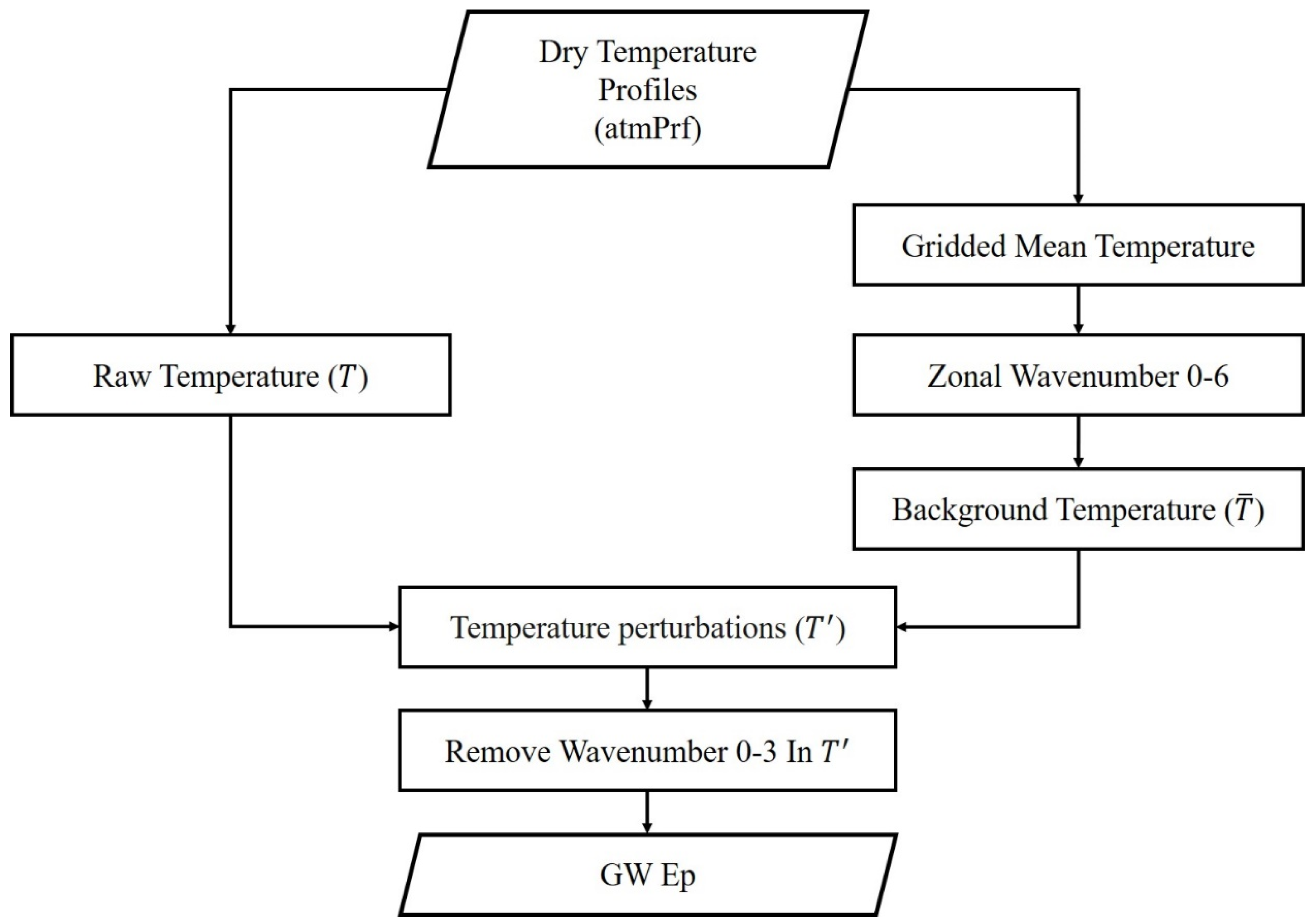
2.2. Method for Extracting GW Activities from RO Temperature Profiles

In the research on the characteristics and distribution patterns of GW activities based on satellite observation data, GW activities are often measured by GW energy (e.g., [2,9,16]), which includes kinetic energy (Ek) and potential energy (Ep). According to the linear wave theory, the ratio of the kinetic energy to the potential energy, Ek/Ep, is approximate to a constant in the atmosphere. Therefore, the characteristics of GW activities can be directly characterized by Ep [16,43], and Ep is calculated by the formulas below:
E p = 1 2 g 2 N 2 ( T T ¯ ) 2
N 2 = g T ¯ ( T ¯ z + g c p )
T = T T ¯
where, g , N, c p , z are respectively the gravitational acceleration, the Brunt-Väisälä frequency, the isobaric heating capacity, and the altitude. T ¯ represents the background temperature, and T′ represents the temperature perturbation caused by the GWs. In the present study, for each original atmPrf profile, the corresponding GW Ep profile is derived using the horizontal detrending method brought forward by Wang and Alexander [21,37], and its flow chart is shown in Figure 1.
The original RO dry temperature profile is of the vertical resolution varying from tens of meters to around a hundred meters, and in the data processing, each temperature profile is interpolated with a height interval of 0.1 km between 20 and 35 km, at first. Then, the daily dry temperature profiles are binned into 15° × 10° longitude–latitude grids, and the mean temperature profile of each grid is derived and then used to construct a three-dimensional single day global temperature grid data. Next, at each height level, S-transform is applied on each zonal component in the global temperature grid data of the single day to derive the zonal wavenumbers, 0–6 of the corresponding latitude band, which are used to construct the three-dimensional background temperature’s grid data. By interpolating back to the positions of the raw temperature profiles in the background temperature’s grid data, the background temperature profiles T ¯ corresponding to the raw temperature profiles are obtained. The profiles of temperature perturbations, T′, are further extracted by subtracting the background temperatures from the raw temperatures using Equation (3). In the next step, S-transform is applied the second time to filter out the 0–3 wavenumber in T′, which aims to remove the residual background information in the temperature perturbations. Finally, the GW Ep is calculated using Equations (1) and (2). What needs to be mentioned is that, theoretically, the GWs with vertical wavelengths longer than twice the vertical resolution of the GNSS RO data (~1km), can be resolved in the present analyses [37].

2.3. Data Quality Check

In our experiment, each atmPrf profile undergoes a two-step quality check. In the first step, the “global attribute” of the original atmPrf profile is checked to eliminate the error profiles which are marked as “bad” by CDAAC. In the next step, the corresponding GW Ep profile is further checked by its maximal and minimal values in the altitude range of 20–35 km. Specifically, if the maximal value in an Ep profile is higher than 50 J/kg or the minimal value is lower than 0 J/kg, this profile is considered to be non-physical, and is thus eliminated [44]. Table 1 presents the number of the original atmPrf profiles, the number of the profiles remained after the global attribute check, and the number of the qualified GW Ep profiles finally obtained from each of the RO missions during 2007 to 2020. A total of 12,247,106 dry temperature profiles from all GNSS RO missions are used in the experiment, among which 10,767,609 profiles remained after the global attribute check and are then used to calculate the GW Ep profiles. Finally, 10,736,341 qualified GW Ep profiles pass through the threshold check of Ep values. In the quality check step 1 and 2, 1,479,497 (12.08%) error profiles and 31,268 (0.26%) non-physical profiles are eliminated, respectively.
The spatial distribution and the annual histogram of the number of the qualified GW Ep profiles derived from all the RO observations during 2007–2020 are shown in Figure 2. Figure 2a presents the spatial distribution of the number of the qualified GW Ep profiles derived from RO data after being binned into 15° × 10° longitude—latitude grids. It can be seen that the number of the retrieved GW Ep profiles in the polar regions of 80° N/S–90° N/S is relatively small (<8000 in each grid), while other regions are generally covered by much more GW Ep profiles. The RO-derived GW Ep profiles in the mid-latitude regions of 20° N/S–60° N/S are particularly dense (>24,000 in each grid). Figure 2b shows the number of the qualified GW Ep profiles derived from each RO mission during different years. As we can see, during 2007 to 2013, the GW Ep profiles are mainly derived from the RO observations of the COSMIC mission, which provides more than 400,000 GW Ep profiles every year. However, after the year 2014, the amount of GW Ep profiles provided by the COSMIC RO observations gradually decreased, due to exceeding the service life of the mission. On the other hand, the METOP-B satellite was launched in the year 2013, and since then, large numbers of GW Ep profiles have been provided by METOP-A/B/C, other than the COSMIC mission. The total number of GW Ep profiles derived from all six RO missions in each year was more than 500,000 during 2007–2020.

2.4. Method for Extracting Long-Term Changes of GW Activities

After obtaining all the qualified GW Ep profiles through the steps introduced in the previous two subsections, these GW Ep profiles are averaged within a single month and binned into 360° × 5° longitude[––]latitude grids, with an overlap of 2.5° in latitude to calculate the monthly and zonal-mean Ep for each height level at the altitude range of 20–35 km. For each latitude band and each height level, the linear trend in monthly zonal-mean Ep time series and the responses of the monthly zonal-mean Ep to solar activity, QBO wind, and ENSO are derived by the method of multivariate linear regression (MLR) [9,45]. The equation for the MLR method is expressed as:
E p ( t i , j ) = μ + α t i , j + β s o l a r ( t i , j ) + γ Q B O ( t i , j ) + κ E N S O ( t i , j ) + R e s i d u a l With   I   = 2007 ,   2008 ,   ,   2020 ;   j   =   1 ,   2 ,   ,   12
In Equation (4), E p ( t i , j ) represents the monthly zonal-mean value of GW Ep at month (j) and year number (i) and the quantity μ represents a constant Ep value. The parameter α, which reflects the change in GW Ep with time, represents the linear trend of monthly zonal-mean Ep during 2007–2020. The parameters β, γ, and κ, which demonstrate the correlation between the time series of GW Ep and the time series of the three indices, represent the responses of the monthly zonal-mean Ep to solar activity, to QBO, and to ENSO. The variance–covariance matrix and student t-test can be used to evaluate whether the estimated regression coefficients are significant at a given confidence level. Giving a significance level s, which means that the corresponding confidence level is set as ( 1 s ) × 100 % , then the corresponding critical value of the t distribution can be obtained in the look-up table. If the absolute value of the ratio between the regression coefficient and its corresponding standard deviation is larger than the critical value of the t distribution at the given significance level s, then it is claimed that the regression coefficient is significant at the confidence level ( 1 s ) × 100 % [46]. In the present study, the confidence level for the t-test is set as 90%.
Figure 3 presents the reference time series of solar activity, QBO, and ENSO during 2007 to 2020. The monthly mean values of radio emissions from the sun at a wavelength of 10.7 centimetres (the 10.7 cm solar flux, F10.7) are used to represent the solar activity [47], and F10.7 is given in solar flux units (sfu, 1   s f u = 10 22   W   m 2   H z 1 ) in Figure 3a. It should be noted that during the studied time period, the solar activity was the most intensive during 2014 to 2015, and declined after the year 2015. In Figure 3b, the temporal variation of 30 hPa zonal-mean zonal wind over the equator is used as the reference time series for QBO [48]. In Figure 3c, the temporal variations of the ENSO phases are shown by the values of the bi-monthly Multivariate El Niño/Southern Oscillation (ENSO) index (MEI), which is the time series of the leading combined Empirical Orthogonal Function (EOF) of five different variables (sea level pressure (SLP), sea surface temperature (SST), zonal and meridional components of the surface wind, and outgoing longwave radiation (OLR)) over the tropical Pacific basin (30° S–30° N and 100° E–70° W) [49,50,51].

3. Results and Analyses

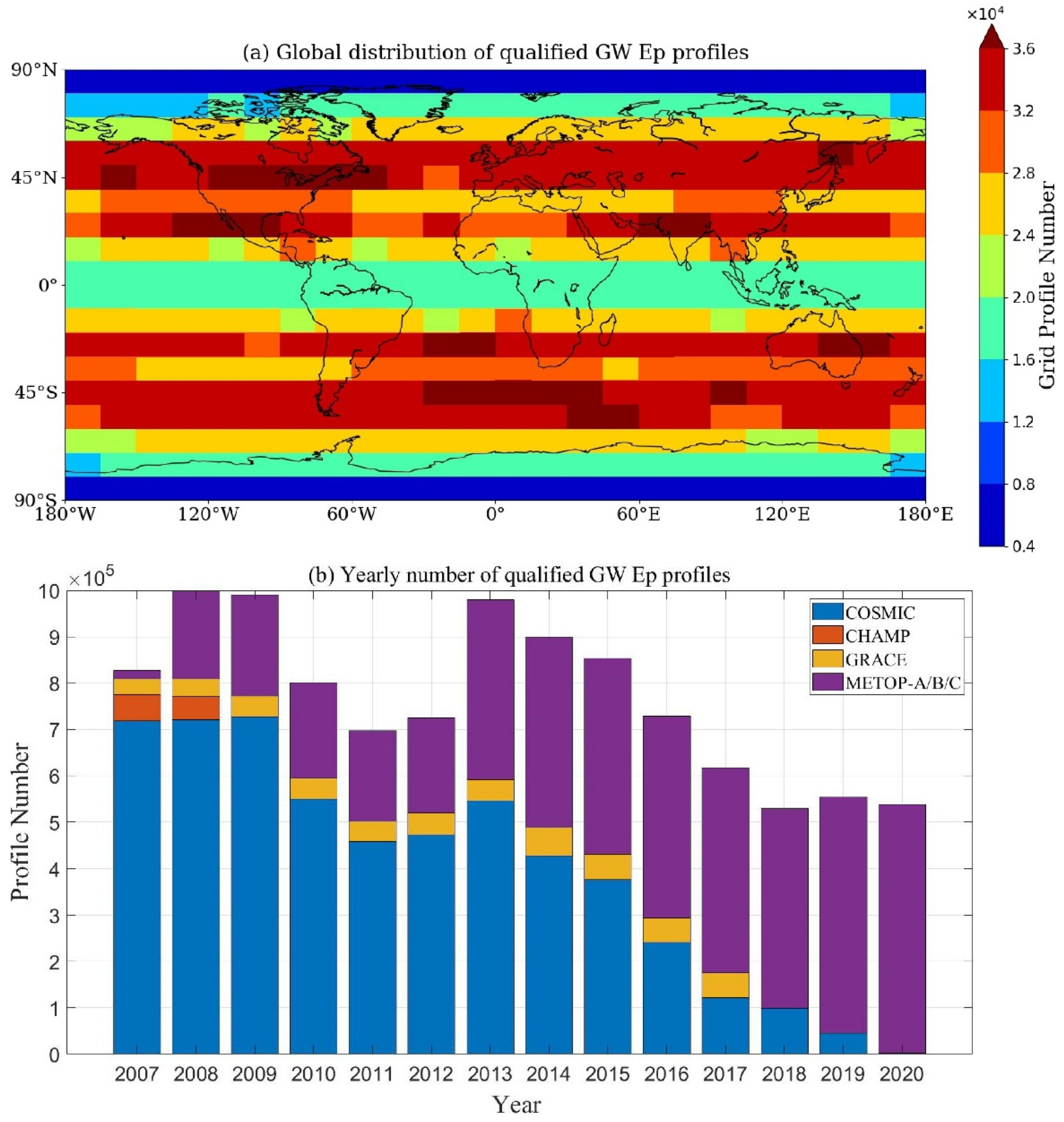
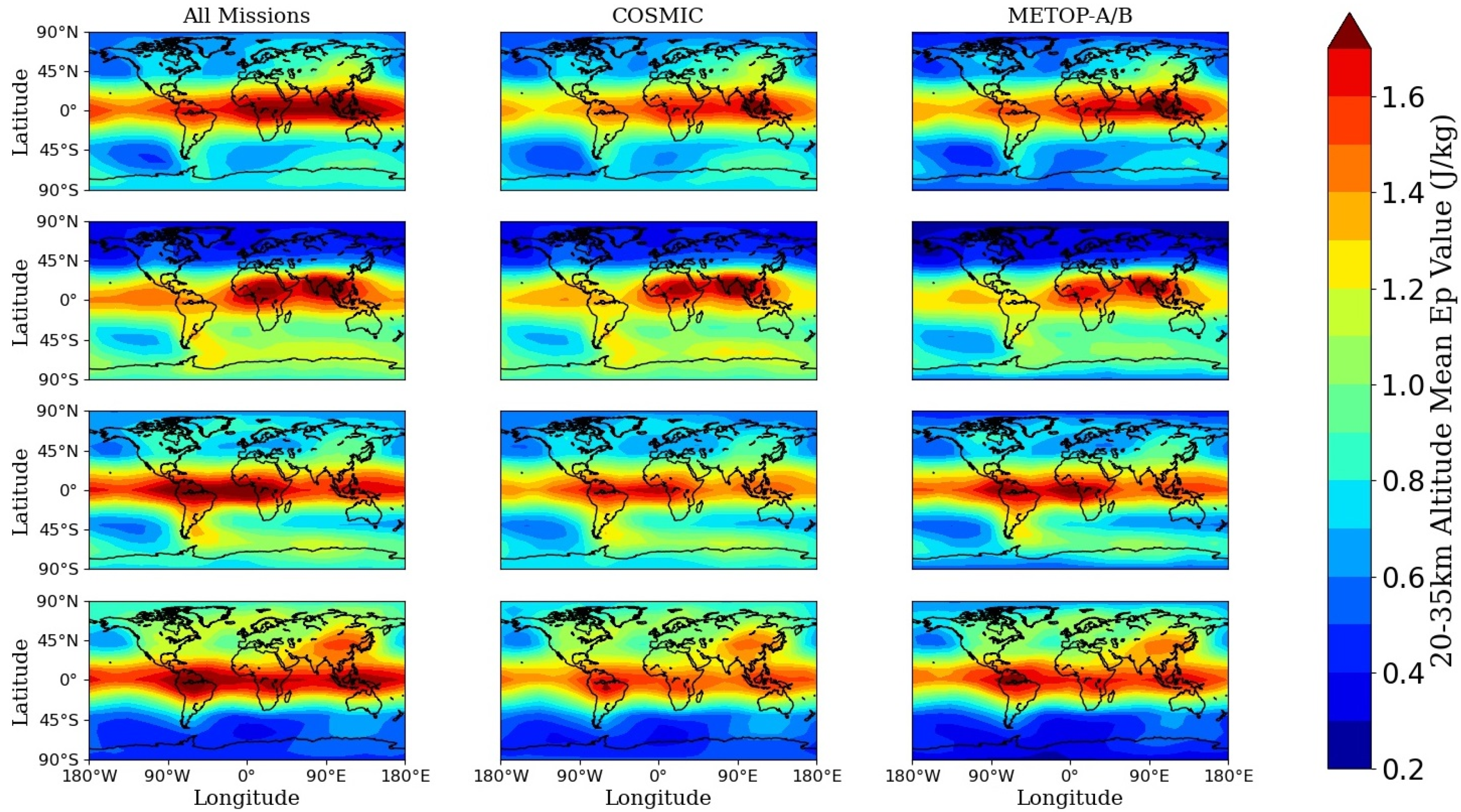
3.1. Comparisons of the Global Distributions of GW Ep Derived from Different RO Datasets

In order to verify the validity of our procedure for deriving the GW Ep values, and to investigate the consistency of the GW Ep values extracted from different RO missions, the seasonal variations of the global distributions of GW Ep at 20–35 km during the period from February 2013 to January 2016 are derived from different datasets and are compared, as shown in Figure 4. Here, the four seasons are categorized as MAM (March to May), JJA (June to August), SON (September to November), and DJF (December to February). The statistics in the subgraphs of the first column are calculated from the profiles of all the missions available for the experiment’s time period (including COSMIC, METOP-A/B, and GRACE), and the subgraphs of the second and third columns are derived from the profiles of COSMIC and METOP-A/B, respectively. The reason why the datasets from February 2013 to January 2016 are selected in this validation experiment is that the Metop-B data series started in February 2013, and COSMIC still provided a sufficient number of profiles every day over the next three years for the statistics of global GW Ep heat map, as shown in Figure 2. The GW Ep seasonal variations derived independently from the GRACE mission are not listed here due to the limited number of temperature profiles provided by GRACE, which is a disadvantage for constructing the single-day geographic grid data to derive the background temperature when applying the horizontal detrending method.
Figure 4 suggests that the magnitudes and the distribution patterns of the GW Ep values derived from the three different datasets, i.e., data of all missions, COSMIC, and METOP-A/B, are of high consistency and the seasonal distribution patterns of the GW values derived from all the three datasets agree well with previous studies [2,52,53,54,55,56,57]. Specifically, the GW Ep values derived from all the three datasets mainly vary between 0.2 to 2 J/kg, and with each of the three datasets, the GW Ep derived is generally higher over the tropical latitude bands than over other regions during all four seasons, and is almost equatorial symmetric in MAM and SON in the tropics. Over the tropics, the distribution of GW Ep is consistent with that of deep convection [17]. In addition, due to the influences of orography and zonal wind, during JJA (the second row)/DJF (the fourth row) in the extratropical regions, the GW Ep values are generally higher over the winter hemisphere than the summer hemisphere [2,9,53,54,57]. Furthermore, for all three datasets, in JJA (the second row) and SON (the third row) we can see a long leeward region of high Ep values exists, which stretches eastward from 70° W to around 180° E, covering the Southern Andes, Drake Passage, and the Antarctic Peninsula. The Ep values over this region reach the maximum in the southern hemisphere (SH) winter and weaken slightly in the SH spring. The eastward propagation of the orographic mountain waves, which is generated by the north–south distribution of the Andes, should contribute to the formation of this specific GW Ep distribution pattern [2,58,59].
The results shown in Figure 4 verify the validity of the procedure for deriving the GW Ep and the feasibility of combining the data from different RO missions in the present study. Moreover, a mixture of datasets from different RO missions was widely used for studying the GW activities in previous studies [21,25,37]. Leroy et al. [60] found that the temperature trends during 2003 to 2014 produced by the combined RO datasets from CHAMP and COSMIC missions and by other satellite observations and model data agree to within 0.02K/year in the lower stratosphere. Therefore, the following analyses of the present work will be carried out using the data from multi-GNSS RO missions simultaneously, and will not differentiate among the data from different RO missions.

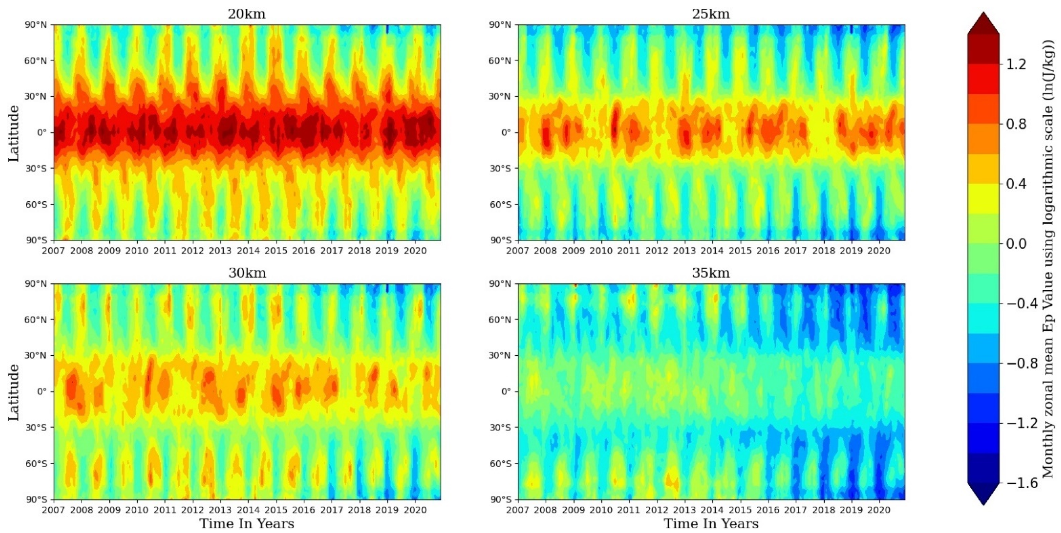
3.2. Time-Latitude Distributions of the Monthly and Zonal-Mean GW Ep

Following the steps mentioned in Section 2.4, the global monthly and zonal-mean GW Ep between 20 and 35 km during 2007 to 2020 are derived, and the time–latitude distributions of the GW Ep values at the four height levels, 20 km, 25 km, 30 km, and 35 km, are derived and are presented in Figure 5 with logarithmic scale.
As we can see, in the altitude range of 20–35 km the values of GW Ep decrease with the increase in altitude, especially in the low latitude area (30° S–30° N). Additionally, at each of the four height levels, the GW Ep shows a clear seasonal cycle. Specifically, over mid and high latitudes, especially in the latitudes higher than 40° N/S, the maximum values of Ep are observed during November–March in the Northern Hemisphere (NH) and May–September in the Southern Hemisphere (SH), which is consistent with previous studies [9,57]. At each of the four height levels, the GW Ep is stronger in high latitudes of the southern winter hemisphere than those of the northern winter hemisphere. The stronger and longer-lasting eastward wind during the winter seasons of the SH compared with the winter seasons of the NH should partly contribute to this distribution pattern of GW Ep values [57,61]. In addition, it can be seen from Figure 5 that after the year 2016, the values of monthly zonal-mean GW Ep decreased compared with previous years, especially at the high level of 35 km.

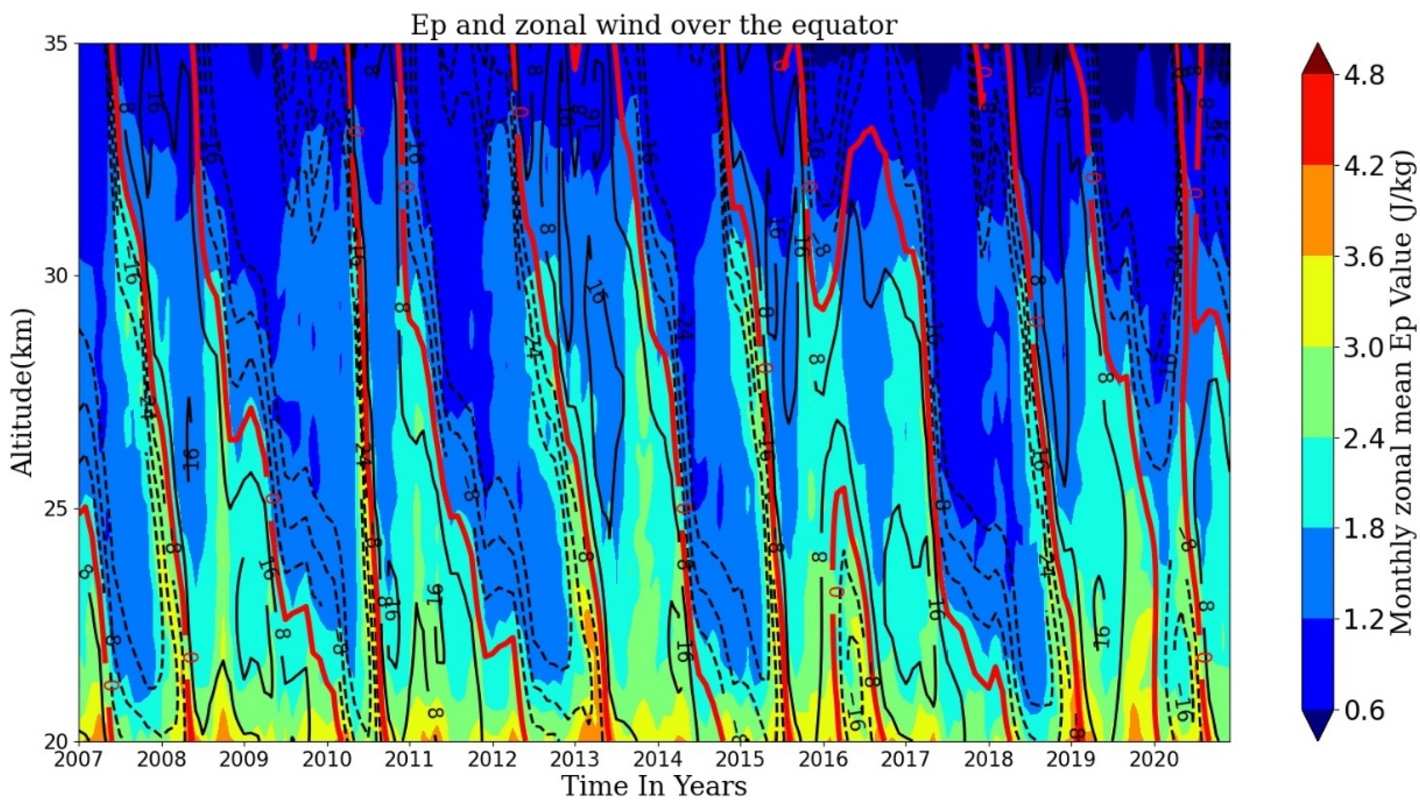
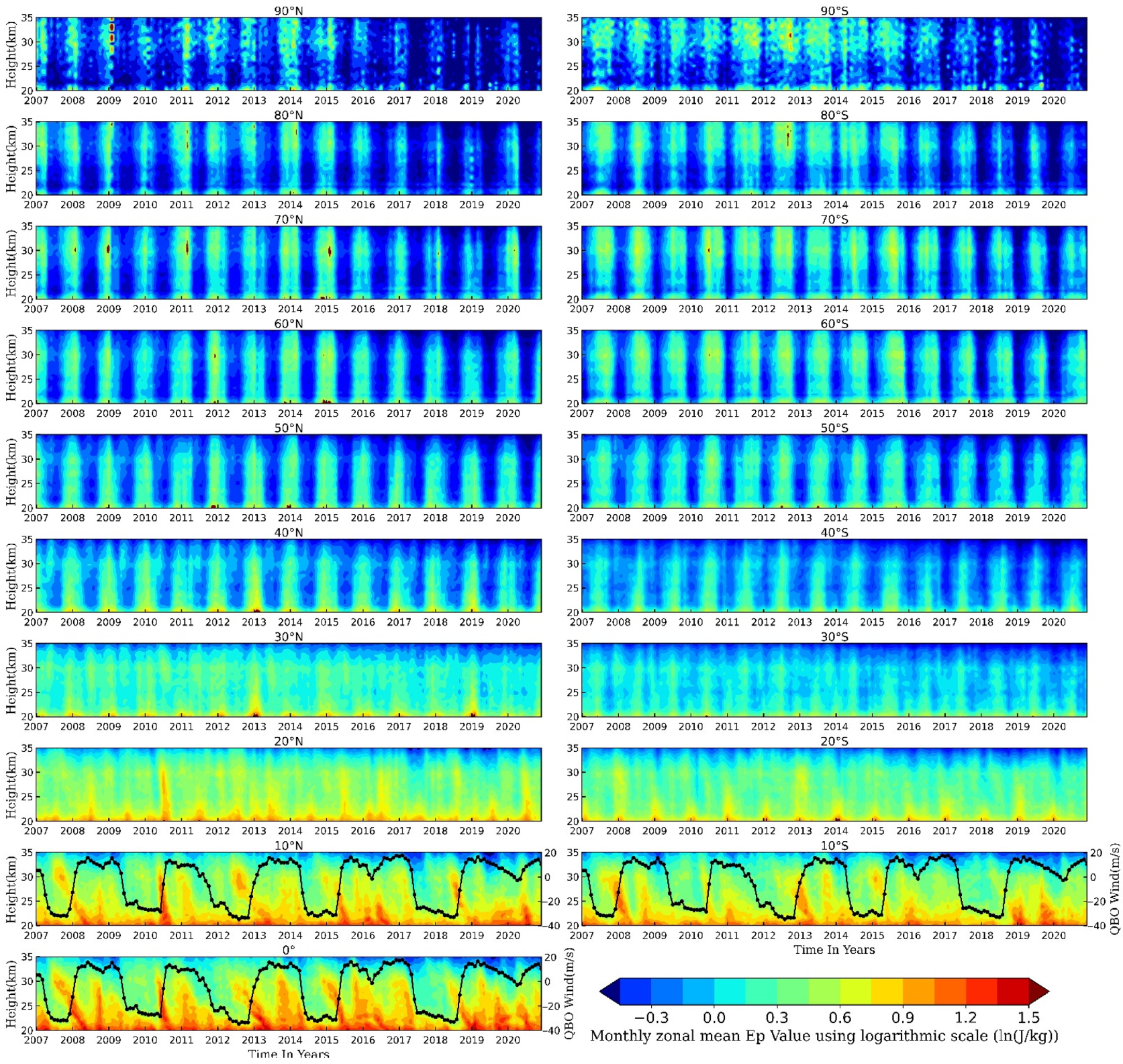
3.3. Time–Height Distributions of the Monthly and Zonal-Mean GW Ep

To investigate the temporal variations of the global GW activities, the time–height distributions of the monthly and global/zonal-mean GW Ep from 2007 to 2020 at 20–35 km height are drawn and are presented using logarithmic scale in Figure 6 and Figure 7, respectively. In these heat maps, the horizontal axis is the time series with the step length of one month, and the vertical axis is the altitude.
As we can see in Figure 6, in general, the magnitudes of the monthly global-mean GW Ep in 20–30 km are greater than those in 30–35 km. The maximum values of the global mean GW Ep appear in the summer solstice and the winter solstice every year, which is the most distinct in 25–30 km. This is consistent with Liu et al. [9], although the altitude range of the GW activity they were concerned about was 30–100 km. Moreover, Figure 6 presents that the magnitudes of GW Ep values before 2016 were significantly larger than those after 2016, which may be related to the sharp weakening in the solar activity during 2015–2017 (shown in Figure 3c), and will be discussed later.
Figure 7 presents the time–height distributions of the monthly zonal-mean GW Ep at different latitudes of the NH (left column) and the SH (right column). The QBO wind time series presented in Figure 3b are overlapped on the Ep distribution at the latitude bands of 10° N/S and the equator. It can be seen that at the latitudes higher than 30° N/S the monthly zonal-mean GW Ep exhibits distinct annual variations, with GW Ep peaks appearing in the winter months of the corresponding hemisphere, which is consistent with the findings of Wilson et al. [62], by using lidar observations in southern France (44° N), and those of Liu et al. [9], by using 14 years of SABER data. The monthly zonal-mean GW Ep exhibits semiannual variations at 20° N/S and 30° N/S, with GW Ep peaks appearing in both the winter and summer months, just similar to the global-mean GW Ep shown in Figure 6.
The QBO signals can be identified in the time variations of GW Ep at 10° N/S and over the equator. The monthly zonal-mean GW Ep at 20–30 km over the tropics peaks when the QBO eastward wind phase reaches its peak too, which is consistent with some previous studies [57,61,63,64]. What needs to be mentioned is that during January 2007 to September 2013, the variation of Ep over the equator shown in Figure 7 is similar to Figure 6 of Xu et al. [57]. By comparing the temporal variations in the GW Ep with those of the zonal wind field, Xu et al. [57] pointed out that, due to the selective filtering effect of stratospheric wind systems on GWs, maximum GW Ep values generally appear where the direction of the wind changes from westward to eastward [63]. The detailed relationship between Ep and zonal wind field over the tropics will be further discussed in Section 4.
At 10° N/S and 20° N/S, the GW Ep has larger values in the summer months than in the winter months, which is consistent with the results of Zhang et al. [64] and Liu et al. [9]. Moreover, at 20° N/S, 30° N/S, and 40° N/S, the zonal-mean GW Ep values at the zonal bands of the NH are larger than those of the corresponding zonal bands of the SH. Using eight-year SABER/TIMED data, Zhang et al. [64] also found that the GW Ep at 10° N–30° N was larger than at 10° S–30° S in 21–26 km height. However, in the latitudes at and higher than 60° N/S, GW activities over the zonal bands of the SH are stronger than those over the corresponding zonal bands of the NH, which has already been described in Section 3.2. In the high latitudes of 70° N/S, 80° N/S, and 90° N/S, GW Ep decreases significantly after 2016, which is shown by the distinct attenuation of the global GW Ep values after 2016 shown in Figure 6.
Figure 6 and Figure 7 present that the temporal variations in the GW Ep change with heights and latitudes. For the altitude range of 20–35 km, in general, the annual variations of GW Ep are prominent at the latitudes higher than 40° N/S, getting peak values in the winter months, while the semiannual variations of GW Ep are distinct at 20–30° N/S, getting peaks both in the winter and the summer months. QBO signals are distinct in the time variations of GW Ep between 10° S–10° N. The above analyses also illustrate that the climatology of GW activities derived above is reliable, based on which the global trends of GWs and the responses of GWs to solar activity, QBO, and ENSO can be further analyzed.

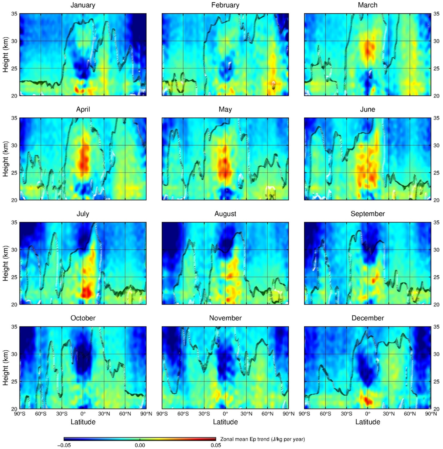
3.4. Global Trends in GWsDuring 2007 to 2020

Following the procedure introduced in Section 2.4, by analyzing the time series of the monthly zonal-mean GW Ep values from 2007 to 2020 with the MLR method, the linear trend (α in Equation (4)) in the GW Ep values for each 2.5°× 0.1 km (latitude× height) grid cell is obtained for each month. For a certain month, if the value of the coefficient α of a grid cell is greater than 0, then the GW Ep of the corresponding cell has a positive trend. Otherwise, the GW Ep of the corresponding cell has a negative trend. The final latitude–height distributions of the GW linear trends for each month are presented in Figure 8. In each subfigure of Figure 8, the regions covering the cells with the trends passing the student t-test with a confidence level of 90% are shown as protuberance.
It can be seen from Figure 8 that in the middle and high latitudes, GW Ep values generally show significant negative trends (<−0.02 J/kg per year) in almost all months, especially in the altitude range of 25–35 km, which is consistent with the phenomena, shown in Figure 5 and Figure 7, that the GW Ep decreases significantly in middle and high latitudes after 2016. Over the tropics, positive trends appear from March to August, while these trends are mostly not significant. Besides, relatively large positive trends appear in the latitudes of 25° N–45° N in November and December, and these trends are not significant either, which is consistent with Liu et al. [9]. The low confidence level of the trends over these latitudes might be partly due to the strong planetary wave activity and the impacts of SSWs in the northern high latitudes. It should be noted that due to the strong extension and subsequent division of the polar vortex, almost the whole NH to the north of about 30° N will be influenced by the enhanced GW activities induced by SSWs [65]. The positive trends occurring in 40° N–70° N during March and April are also consistent with the findings of Liu et al. [9]. In addition, the significant negative trends over 5° N–30° N in January and the negative trends over 25° N–40° N in February in the range of 30–35 km, which were presented in Figure 5 of Liu et al. [9], are also shown here in Figure 8.
Considering that a half-year shift exists in the atmospheric conditions between the two hemispheres, some distinct characteristics of GW trends can be determined, which are almost symmetrical between the SH and the NH. For example, in the altitude range of 30–35 km, both the high latitudes of the SH during June, July, and August and the high latitudes of the NH during December, January, and February have significant negative trends, which are generally lower than –0.03 J/kg per year. In the NH from June to September and in the SH from December to March, the GW Ep values at 25–35 km over the mid-high latitudes generally show significantly negative trends, which are of the magnitudes of –0.01 to –0.03 J/kg per year. Whether for the more active winter months or for the relatively less active summer months of the gravity waves, the GW Ep trends generally show a consistent symmetry over the two hemispheres. Furthermore, the GW activities in 20–35 km are generally declining from 2007 to 2020.
The latitude–height distributions of the deseasonalized trends in the monthly zonal-mean GW Ep values at 20–35 km during 2007 to 2020 and the responses of GW Ep to solar flux, QBO, and ENSO are presented in Figure 9. Similar to Figure 8, in each subfigure of Figure 9, the regions where the results are statistically significant at the confidence level of 90% are shown as protuberance.
The deseasonalized trends shown in Figure 9a are derived by analyzing the deseasonalized monthly zonal-mean GW Ep time series using the MLR method [46,66]. As we can see from Figure 9a, except for a few locations, GW Ep values generally show significant negative trends at most latitudes and altitudes, especially in the middle and high latitudes of the two hemispheres. In addition, in the low latitudes of 30° S–30° N, significant negative trends exist above 30 km. The values of the negative trends become smaller in the regions closer to the poles, which is consistent with what is shown in Figure 8. In the following subsection, we will further analyze the responses of GW to solar activity, QBO wind, and ENSO.

3.5. Responses of GW Activities to Solar Activity, QBO Wind, and ENSO over the Globe

The response of the variation in GW Ep at 20–35 km to that of the solar activity represented by the F10.7 indexes is shown in Figure 9b. Contrary to the GW Ep trends during the 14 years, which are mainly negative, GW Ep in the mid and high latitudes of the two hemispheres generally show significant positive responses to the solar activity within the altitude range of 20–35 km. In the low latitudes of 30° S–30° N, significant positive responses of GW Ep to solar activity also exist at 30–35 km. Additionally, in terms of the magnitudes of the responses, the positive responses of the GW Ep to the solar activity become stronger in the region closer to the poles. Our results are consistent with Jacobi et al. [30], who got positive correlations of GWs with the solar activities by using the radio drift observations at 52° N.
Figure 9c presents the responses of GW activities to QBO at 20–35 km over the globe. It can be seen that at the latitude range of 20–35 km, the responses of GW Ep values to the QBO eastward wind phases are mainly negative at most latitudes. At the altitude range of 30–35 km, significant negative responses of GW Ep to the QBO eastward wind phases occur at the latitudes of 30° S–25° N, and the negative responses at 0°–25° N are smaller than those at 0°–30° S, which is basically consistent with Liu et al. [9]. At the altitude range of 20–30 km, the significant negative responses extend to the mid and high latitudes in the SH, while at the low latitudes of 15° S–15° N, the responses of GW Ep values to the QBO eastward wind phases are significantly positive.
The response of the GW Ep at 20–35 km to ENSO, which is represented by the MEI index, is shown in Figure 9d. It can be seen that over low latitudes of 15° S–15° N, GW Ep values are of positive responses to ENSO in 20–35 km, which is consistent with Liu et al. [9]. In addition, the response of the GW Ep to ENSO is significantly negative in 30–35 km over the latitudes of 15° N–30° N, which is also consistent with the findings of Liu et al. [9]. The significant negative response near 50° N in our results should be partly due to the weakening in GW activity after 2016.

4. Discussion

The comparison between Figure 9a,b demonstrates that the height–latitude distribution pattern of the trends in the GW Ep and that of the response of GW Ep to the solar activity show distinct correlations, i.e., the overall negative trends in GWs correspond to the overall positive responses of the GW Ep to the solar activity. Considering that the solar activity weakened significantly after the year 2015, as shown in Figure 3a, it can be deduced that the sharp decline in the solar activity after the year 2015, together with the positive response of the GW Ep to the solar activity, might have contributed significantly to the overall attenuation of the gravity wave activity during the 14 years from 2007 to 2020. What needs to be mentioned is that Ern et al. [67] and Liu et al. [9] both observed negative responses in GW Ep to F10.7 indexes at the altitude range of 30–35 km above low and middle latitudes by using the SABER temperature data, which are different from our results, while the time periods researched by Ern et al. [67] and by Liu et al. [9] are 2002–2011 and 2002–2015, respectively, and the F10.7 data after the year 2015 were not used in their studies. Moreover, Gavrilov et al. [29] pointed out that differences in GW sources, in conditions of wave propagations, and in measurement methods might all have impacts on the analyses concerning the responses of GW to solar activities. We suggest that a possible reason why our results are inconsistent with those of Ern et al. [67] and Liu et al. [9] is that the solar activity weakened sharply during 2015 to 2017 (as shown in Figure 3a), which partially contributed to the general weakening of GW activities after 2016.
The specific dynamic mechanisms which directly lead to the negative trend in global GW Ep are still unclear. Considering that the significant negative trend is particularly notable in the polar regions, these background dynamic mechanisms might be related to the enhancement/weakening of polar circulations or the expansion and break in polar vortexes. On the other hand, as shown in Figure 5 and Figure 7, the GW Ep at high latitudes has been declining extremely rapidly since 2016, accompanied by a decrease in solar activity. Taking into consideration the strong positive correlation between GW Ep and solar activity revealed in the present study, it is speculated that the dynamic mechanisms which lead to the negative trend in global GW Ep should also be strongly affected by the solar activity. More work will be done on this issue in our future work.
The comparisons of the QBO time series, the time–height distributions of the monthly and zonal-mean GW Ep over the equator, and the latitudes of 10° N and 10° S, which are presented in Figure 7, reveal that during the time periods when peak values appear in the QBO eastward wind phase time series, the monthly zonal-mean GW Ep values in 20–30 km also reach peak values over the equator and over 10° N/S, where the value of ln(Ep) is larger than 0.6 ln(J/kg) and is shown with red color in Figure 7. Figure 10 further presents the time–height cross section of Ep and zonal wind field at 20–35 km over the equator during 2007 and 2020. As mentioned in Section 3.3, due to the selective filtering effect of stratospheric wind systems on GWs, the GW Ep value above the 0 m s−1 wind level line is usually significantly attenuated compared with the value below it. We also can see that the Ep value at 20–30 km is generally large (>1.8 J/kg) in the eastward wind time period and small (<1.8 J/kg) in the westward wind time period. This is a manifestation of the significant positive correlation between the GW Ep in the altitude range of 20–30 km and the QBO over the tropics, and is consistent with the significant positive responses of GW Ep below 30 km over 15° S–15° N, as shown in Figure 9c. This indicates that GW Ep activity in 20–30 km over the tropics is mainly affected by the variation in the zonal wind field. In addition, Figure 7 also shows that during the two peak periods of QBO east wind phases from March 2015 to June 2017 and from June 2018 to December 2020, the values of GW Ep at 30–35 km over the equator and over 10° N/S are at a lower level compared with other peak periods, which might lead to the negative response of GW activity to QBO within 30–35 km height over the tropics.
A possible mechanism for explaining the positive response of GW activities to ENSO over the low latitudes is that convective GW sources in the tropical region may be strengthened by the El Niño events, which change the atmospheric wind and temperature structures [68,69]. What needs to be mentioned is that, at the altitude range of 30–35 km over the latitudes near 50° N, GW Ep has a significant negative response to ENSO in our results, while in the work of Liu et al. [9], significant positive responses are found at the same region. The difference between ours and Liu et al.’s results should be mainly attributed to the different time periods of the two studies. The time period focused on by Liu et al. [9] was 2002–2015, while our work focused on the period from 2007 to 2020.

5. Conclusions

By using multi-mission GNSS RO data from 2007 to 2020, the present study studies the variations in the gravity waves at the lower stratosphere of 20–35 km over the globe. The dry temperature profiles (atmPrf files) from six different RO missions provided by CDAAC, after a two-step quality check, are used to retrieve the GW Ep profiles, based on which the temporal variations of the GW activities are derived and the linear trends of the GWs and the responses of GW activities to solar activity, QBO, and ENSO are further analyzed using the MLR method.
To verify the validity of our procedure for extracting the GW Ep profiles with the horizontal detrending method and to understand the consistency of the GWs derived from different RO missions, firstly, the global distributions of the seasonal means of GW Ep values at the altitude range of 20–35 km, derived respectively from three RO datasets, i.e., data of all the missions, COSMIC data only, and METOP-A/B data only, during the period from February 2013 to January 2016, are compared. It is found that the distribution patterns of the seasonal means of GW Ep values derived from the three datasets are all consistent with previous works, and there are no significant differences among the magnitudes of the Ep values derived from different RO datasets, which confirms the feasibility of the method for extracting the GW Ep and suggests that it is statistically reasonable to use the data from multi-GNSS RO missions to study the trend in the GW activities.
By analyzing the time–latitude and the time–height distributions of the GW Ep values during the 14 years from 2007 to 2020, we found that GW activities in 20–35 km show distinct annual variations in mid and high latitude regions with latitudes higher than 40° in both of the two hemispheres, reaching the peaks during winter months of the corresponding hemisphere. The stronger and longer-lasting eastward wind during the winter seasons of the SH compared with the winter seasons of the NH should partly contribute to the GW Ep distribution pattern that GW activities are stronger in winter months at high latitudes of the SH than that of the NH. At lower latitudes of 20° N/S and 30° N/S, GW activities at the altitudes of 20–35 km exhibit semiannual variations, with Ep values peaking in both winter and summer months. At the equator and the latitudes of 10° N/S, QBO signals of GW Ep are observed, which should be related to the selective filtration of gravity waves by the stratospheric wind system. Moreover, the zonal-mean GW activities over the latitudes of 20° N, 30° N, and 40° N are generally larger than those of the same latitude bands of the SH, which is contrary to the comparison between the high latitudes of the two hemispheres. In addition, in both the time–latitude and the time–altitude distributions of the GW Ep values, it is clearly observed that in high latitude regions, there has been a significant decrease in the strength of the GW activities since 2016.
From the latitude–height distributions of the trends in the GW Ep values during each month, it is found that positive, while not significant, trends appear from March to August over the tropics. Being consistent with Liu et al. [9], relatively large positive trends which are not significant appear in the latitudes of 25° N–45° N in November and December, and positive trends also occur in the latitudes of 40° N–70° N during March and April. Moreover, in the altitude range of 25–35 km of the middle and high latitudes, GW Ep values generally show significant negative trends in almost all months, and the values of the negative trends become smaller in the region closer to the poles. A similar pattern is also shown in the distribution of the deseasonalized trends of monthly zonal-mean GW Ep time series during the 14 years from 2007 to 2020. Furthermore, some prominent features, which are almost symmetric between the NH and the SH, can be figured out in the distributions of the GW Ep trends of different months when taking into consideration the six months shift in the atmospheric conditions between the two hemispheres. On the whole, the gravity wave activities are declining from 2007 to 2020 over the globe.
The analyses concerning the responses of the global GW activities in 20–35 km to solar activity, QBO, and ENSO during 2007 to 2020 reveal that the responses of GW Ep values to solar activity are mostly positive. The latitude–height distribution of the areas with significant responses are very similar to that of the deseasonalized trends of the GW Ep, and the positive responses of the GW Ep to solar activity become stronger in the regions closer to the poles. The comparison between the distribution pattern of the deseasonalized trends of the GW activities and that of the response of GW activities to solar activity indicates that the sharp decline in solar activity from 2015 to 2017 might contribute to the overall attenuation of gravity wave activity during the 14 years from 2007 to 2020. Furthermore, significant negative responses of the GW activities to QBO are found in 30–35 km over the latitudes of 30° S–25° N, and the negative responses extend to the mid and high latitudes in the SH at 20–30 km. Meanwhile, the responses of GW activities to QBO change to be significantly positive in 20–30 km over the latitudes of 15° S–15° N, which demonstrates that the variation in the zonal wind field should be the main factor affecting the GW activities in 20–30 km over the tropics. The responses of GW activities to ENSO at 20–35 km are found to be positive over the latitudes of 15° S–15° N, while at 30–35 km over 15° N–30° N and at 20–35 km near the latitude of 50° N, significant negative responses of GW activities to ENSO exist.

Author Contributions

Conceptualization, X.X.; Investigation, J.L. and J.H.; Methodology, J.H.; Project administration, J.L. and X.X.; Supervision, J.L. and X.X.; Writing—original draft, J.L. and J.H.; Writing—review and editing, X.X. All authors have read and agreed to the published version of the manuscript.

Funding

This work is supported by the National Natural Science Foundation of China (Grant Nos. 41774033, 41774032, and 42074027).

Data Availability Statement

The data used in the manuscript are all public data. The atmPrf data of the RO missions, including CHAMP, COSMIC, GRACE, and METOP-A/B/C, were downloaded from the CDAAC Data Center: https://cdaac-www.cosmic.ucar.edu/cdaac/products.html (last accessed on 27 August 2021). The F10.7 data were downloaded from the Canadian Space Weather Forecast Centre: https://www.spaceweather.gc.ca/solarflux/sx-5-en.php (last accessed on 27 August 2021), QBO data were downloaded from the Institute of Meteorology of Freie Universität Berlin: http://www.geo.fu-berlin.de/en/met/ag/strat/produkte/qbo/ (last accessed on 27 August 2021), and MEI data were downloaded from the NOAA Physical Sciences Laboratory http://www.esrl.noaa.gov/psd/enso/mei/ (last accessed on 27 August 2021). The ERA5 reanalysis dataset was downloaded from the ECMWF: https://www.ecmwf.int/en/forecasts/datasets/reanalysis-datasets/era5 (last accessed on 27 August 2021).

Acknowledgments

The authors would like to express their gratitude to University Corporation for Atmospheric Research (UCAR) for providing the GNSS RO data. We are also very grateful to the Canadian Space Weather Forecast Centre, the Institute of Meteorology of Freie Universität Berlin, the NOAA Physical Sciences Laboratory, and the ECMWF for providing the data of F10.7, QBO, MEI, and the ERA5 reanalysis dataset, respectively.

Conflicts of Interest

The authors declare no conflict of interest.

References

  1. Fritts, D.C.; Alexander, M.J. Gravity wave dynamics and effects in the middle atmosphere. Rev. Geophys. 2003, 41, 1003. [Google Scholar] [CrossRef] [Green Version]
  2. Hindley, N.P.; Wright, C.J.; Smith, N.D.; Mitchell, N.J. The southern stratospheric gravity wave hot spot: Individual waves and their momentum fluxes measured by COSMIC GPS-RO. Atmos. Chem. Phys. 2015, 15, 7797–7818. [Google Scholar] [CrossRef] [Green Version]
  3. Uccellini, L.W.; Koch, S.E. The synoptic setting and possible energy sources for mesoscale wave disturbances. Mon. Weather Rev. 1987, 115, 721–729. [Google Scholar] [CrossRef] [Green Version]
  4. Manzini, E.; McFarlance, N.A. The effect of varying the source spectrum of a gravity wave parameterization in a middle atmosphere general circulation model. J. Geophys. Res. 1998, 103, 31523–31540. [Google Scholar] [CrossRef]
  5. Liu, H.L.; Hays, P.B.; Roble, R.G. A numerical study of gravity wave breaking and impacts on turbulence and mean state. J. Atmos. Sci. 1999, 56, 2152–2177. [Google Scholar] [CrossRef]
  6. Xu, J.; Smith, A.K.; Collins, R.L.; She, C.Y. Signature of an overturning gravity wave in the mesospheric sodium layer: Comparison of a nonlinear photochemical-dynamical model and lidar observations. J. Geophys. Res. 2006, 111, D17301. [Google Scholar] [CrossRef]
  7. Kim, Y.; Eckermann, S.D.; Chun, H. An overview of the past, present and future of gravity-wave drag parametrization for numerical climate and weather prediction models. Atmos. Ocean 2003, 41, 65–98. [Google Scholar] [CrossRef]
  8. Alexander, S.P.; Shepherd, M.G. Planetary wave activity in the polar lower stratosphere. Atmos. Chem. Phys. 2010, 10, 707–718. [Google Scholar] [CrossRef] [Green Version]
  9. Liu, X.; Yue, J.; Xu, J.; Garcia, R.R.; Russell Ⅲ, J.M.; Mlynczak, M.; Wu, D.L.; Nakamura, T. Variations of global gravity waves derived from 14 years of SABER temperature observations. J. Geophys. Res. Atmos. 2017, 122, 6231–6249. [Google Scholar] [CrossRef]
  10. Watanabe, S.; Kawatani, Y.; Tomikawa, Y.; Miyazaki, K.; Takahashi, M.; Sato, K. General aspects of a T213L256 middle atmosphere general circulation model. J. Geophys. Res. 2008, 113, D12110. [Google Scholar] [CrossRef] [Green Version]
  11. Liu, H.L.; McInerney, J.M.; Santos, S.; Lauritzen, P.H.; Taylor, M.A.; Pedatella, N.M. Gravity waves simulated by high-resolution Whole Atmosphere Community Climate Model. Geophys. Res. Lett. 2014, 41, 9106–9112. [Google Scholar] [CrossRef] [Green Version]
  12. Holt, L.A.; Alexander, M.J.; Coy, L.; Molod, A.; Putman, W.; Pawson, S. Tropical waves and the quasi-biennial oscillation in a 7-km global climate simulation. J. Atmos. Sci. 2016, 73, 3771–3783. [Google Scholar] [CrossRef]
  13. Kursinski, E.R.; Hajj, G.A.; Schofield, J.T.; Linfield, R.P.; Hardy, K.R. Observing Earth’s atmosphere with radio occultation measurements using the Global Positioning System. J. Geophys. Res. Atmos. 1997, 102, 23429–23465. [Google Scholar] [CrossRef]
  14. Steiner, A.K.; Kirchengast, G. Error analysis for GNSS radio occultation data based on ensembles of profiles from end-to-end simulations. J. Geophys. Res. 2005, 110, D15307. [Google Scholar] [CrossRef]
  15. Horinouchi, T.; Tsuda, T. Spatial structures and statistics of atmospheric gravity waves derived using a heuristic vertical cross-section extraction from COSMIC GPS radio occultation data. J. Geophys. Res. Atmos. 2009, 114, D16. [Google Scholar] [CrossRef] [Green Version]
  16. Tsuda, T.; Nishida, M.; Rocken, C.; Ware, R.H. A global morphology of gravity wave activity in the stratosphere revealed by the GPS occultation data (GPS/MET). J. Geophys. Res. 2000, 105, 7257–7273. [Google Scholar] [CrossRef]
  17. Ratnam, M.V.; Tetzlaff, G.; Jacobi, C. Global and seasonal variations of stratospheric gravity wave activity deduced from the CHAMP/GPS satellite. J. Atmos. Sci. 2004, 61, 1610–1620. [Google Scholar] [CrossRef]
  18. Ratnam, M.V.; Tsuda, T.; Jacobi, C.; Aoyama, Y. Enhancement of gravity wave activity observed during a major southern hemisphere stratospheric warming by CHAMP/GPS measurements. Geophys. Res. Lett. 2004, 31, 171–184. [Google Scholar]
  19. Alexander, S.P.; Tsuda, T.; Kawatani, Y. COSMIC GPS observations of northern hemisphere winter stratospheric gravity waves and comparisons with an atmospheric general circulation model. Geophys. Res. Lett. 2008, 35, 156–167. [Google Scholar] [CrossRef]
  20. Alexander, S.P.; Tsuda, T.; Kawatani, Y.; Takahashi, M. Global distribution of atmospheric waves in the equatorial upper troposphere and lower stratosphere: COSMIC observations of wave mean flow interactions. J. Geophys. Res. 2008, 113, D24115. [Google Scholar] [CrossRef]
  21. Wang, L.; Alexander, M.J. Global estimates of gravity wave parameters from GPS radio occultation temperature data. J. Geophys. Res. Atmos. 2010, 115, D21122. [Google Scholar] [CrossRef]
  22. Kohma, M.; Sato, K. The effects of atmospheric waves on the amounts of polar stratospheric clouds. Atmos. Chem. Phys. 2011, 11, 11535–11552. [Google Scholar] [CrossRef] [Green Version]
  23. Faber, A.; Llamedo, P.; Schmidt, T.; De, L.; Wickert, J. A new approach to global gravity wave momentum flux determination from GPS radio occultation data. Atmos. Meas. Tech. Discuss. 2013, 6, 2907–2933. [Google Scholar] [CrossRef] [Green Version]
  24. Tsuda, T. Characteristics of atmospheric gravity waves observed using the MU (Middle and Upper atmosphere) radar and GPS (Global Positioning System) radio occultation. Proc. Jpn. Acad. Ser. B 2014, 90, 12–27. [Google Scholar] [CrossRef] [Green Version]
  25. Schmidt, T.; Alexander, P.; de la Torre, A. Stratospheric gravity wave momentum flux from radio occultations. J. Geophys. Res. Atmos. 2016, 121, 4443–4467. [Google Scholar] [CrossRef] [Green Version]
  26. Hoffmann, P.; Rapp, M.; Singer, W.; Keuer, D. Trends of mesospheric gravity waves at northern middle latitudes during summer. J. Geophys. Res. 2011, 116, D00P08. [Google Scholar] [CrossRef] [Green Version]
  27. Gavrilov, N.M.; Riggin, D.M.; Fritts, D.C. Interannual variations of the mean wind and gravity wave variances in the middle atmosphere over Hawaii. J. Atmos. Sol. Terr. Phys. 2004, 66, 637–645. [Google Scholar] [CrossRef]
  28. Gavrilov, N.M.; Manson, A.H.; Meek, C.E. Climatological monthly characteristics of middle atmosphere gravity waves (10 min-10 h) during 1979–1993 at Saskatoon. Ann. Geophys. 1995, 13, 285–295. [Google Scholar]
  29. Gavrilov, N.M.; Fukao, S.; Nakamura, T.; Jacobi, C.; Kürschner, D.; Manson, A.H.; Meek, C.E. Comparative study of interannual changes of the mean winds and gravity wave activity in the middle atmosphere over Japan, Central Europe and Canada. J. Atmos. Sol. Terr. Phys. 2002, 64, 1003–1010. [Google Scholar] [CrossRef]
  30. Jacobi, C.; Gavrilov, N.M.; Kürschner, D.; Fröhlich, K. Gravity wave climatology and trends in the mesosphere/lower thermosphere region deduced from low-frequency drift measurements 1984–2003 (52.1° N, 13.2° E). J. Atmos. Sol. Terr. Phys. 2006, 68, 1913–1923. [Google Scholar] [CrossRef]
  31. Li, T.; Leblanc, T.; McDermid, I.S.; Wu, D.L.; Dou, X.; Wang, S. Seasonal and interannual variability of gravity wave activity revealed by long-term lidar observations over Mauna Loa Observatory, Hawaii. J. Geophys. Res. 2010, 115, D13103. [Google Scholar] [CrossRef] [Green Version]
  32. Wickert, J.; Reigber, C.; Beyerle, G.; König, R.; Marquardt, C.; Schmidt, T.; Grunwaldt, L.; Galas, R.; Meehan, T.K.; Melbourne, W.G.; et al. Atmosphere sounding by GPS radio occultation: First results from CHAMP. Geophys. Res. Lett. 2001, 28, 3263–3266. [Google Scholar] [CrossRef] [Green Version]
  33. Anthes, R.A.; Bernhardt, P.A.; Chen, Y.; Cucurull, L.; Dymond, K.F.; Ector, D.; Healy, S.B.; Ho, S.P.; Hunt, D.C.; Kuo, Y.H.; et al. The COSMIC/FORMOSAT-3 mission: Early results. Bull. Am. Meteorol. Soc. 2008, 89, 313–334. [Google Scholar] [CrossRef]
  34. Beyerle, G.; Schmidt, T.; Michalak, G.; Heise, S.; Wickert, J.; Reigber, C. GPS radio occultation with GRACE: Atmospheric profiling utilizing the zero difference technique. Geophys. Res. Lett. 2005, 32, L13806. [Google Scholar] [CrossRef] [Green Version]
  35. Von Engeln, A.; Andres, Y.; Marquardt, C.; Sancho, F. GRAS radio occultation on-board of Metop. Adv. Space Res. 2011, 47, 336–347. [Google Scholar] [CrossRef]
  36. Righetti, P.L.; de Juana Gamo, J.M.; Sancho, F. Metop-C deployment and start of three-satellite operations. Aeronaut. J. 2020, 124, 902–916. [Google Scholar] [CrossRef]
  37. Wang, L.; Alexander, M.J. Gravity wave activity during stratospheric sudden warmings in the 2007–2008 Northern Hemisphere winter. J. Geophys. Res. 2009, 114, D18108. [Google Scholar] [CrossRef]
  38. Tsuda, T.; Lin, X.; Hayashi, H.; Noersomadi. Analysis of vertical wave number spectrum of atmospheric gravity waves in the stratosphere using COSMIC GPS radio occultation data. Atmos. Meas. Tech. 2011, 4, 1627–1636. [Google Scholar] [CrossRef] [Green Version]
  39. Hajj, G.A.; Ao, C.O.; Iijima, B.A.; Kuang, D.; Kursinski, E.R.; Mannucci, A.J.; Meehan, T.K.; Romans, L.J.; de la Torre Juarez, M.; Yunck, T.P. CHAMP and SAC-C atmospheric occultation results and intercomparisons. J. Geophys. Res. Atmos. 2004, 109, D06109. [Google Scholar] [CrossRef]
  40. Wickert, J.; Michalak, G.; Schmidt, T.; Beyerle, G.; Cheng, C.Z.; Healy, S.B.; Heise, S.; Huang, C.Y.; Jakowski, N.; Köhler, W.; et al. GPS radio occultation: Results from CHAMP, GRACE and FORMOSAT-3/COSMIC. Terr. Atmos. Ocean. Sci. 2009, 20, 35–50. [Google Scholar] [CrossRef] [Green Version]
  41. Schreiner, W.; Sokolovskiy, S.; Hunt, D.; Rocken, C.; Kuo, Y.H. Analysis of GPS radio occultation data from the FORMOSAT-3/COSMIC and Metop/GRAS missions at CDAAC. Atmos. Meas. Tech. 2011, 4, 2255–2272. [Google Scholar] [CrossRef] [Green Version]
  42. Ho, S.P.; Peng, L.; Vömel, H. Characterization of the longterm radiosonde temperature biases in the upper troposphere and lower stratosphere using COSMIC and Metop-A/GRAS data from 2006 to 2014. Atmos. Chem. Phys. 2017, 17, 4493–4511. [Google Scholar] [CrossRef] [Green Version]
  43. Fritts, D.C.; VanZandt, T.E. Spectral estimates of gravity wave energy and momentum fluxes. Part I: Energy dissipation, acceleration, and constraints. J. Atmos. Sci. 1993, 50, 3685–3694. [Google Scholar] [CrossRef]
  44. Xu, X.; Yu, D.; Luo, J. Seasonal variations of global stratospheric gravity wave activity revealed by COSMIC RO data. In Proceedings of the CPGPS 2017 Forum on Cooperative Positioning and Service, Harbin, China, 19–21 May 2017. [Google Scholar]
  45. Gao, P.; Xu, X.; Zhang, X. Characteristics of the trends in the global tropopause estimated from cosmic radio occultation data. IEEE Trans. Geosci. Remote. Sens. 2015, 53, 6813–6822. [Google Scholar] [CrossRef]
  46. Kutner, M.H.; Nachtsheim, C.J.; Neter, J.; Li, W. Applied Linear Statistical Models, 5th ed.; Mcgraw-Hill/Irwin: San Francisco, CA, USA, 2004; pp. 40–88 and pp. 214–247. [Google Scholar]
  47. Tapping, K.F. The 10.7 cm solar radio flux (F10.7). Space Weather 2013, 11, 394–406. [Google Scholar] [CrossRef]
  48. Baldwin, M.P.; Gray, L.J.; Dunkerton, T.J.; Hamilton, K.; Haynes, P.H.; Randel, W.J.; Holton, J.R.; Alexander, M.J.; Hirota, I.; Horinouchi, T. The quasi-biennial oscillation. Rev. Geophys. 2001, 39, 179–229. [Google Scholar] [CrossRef]
  49. Randel, W.J.; Garcia, R.R.; Calvo, N.; Marsh, D. ENSO influence on zonal mean temperature and ozone in the tropical lower stratosphere. Geophys. Res. Lett. 2009, 36, L15822. [Google Scholar] [CrossRef] [Green Version]
  50. Wolter, K.; Timlin, M.S. El Niño/Southern Oscillation behaviour since 1871 as diagnosed in an extended multivariate ENSO index (MEI.ext). Int. J. Climatol. 2011, 31, 1074–1087. [Google Scholar] [CrossRef]
  51. Li, T.; Calvo, N.; Yue, J.; Dou, X.; Russell, J.M., III; Mlynczak, M.G.; She, C.Y.; Xue, X. Influence of El Niño-Southern Oscillation in the mesosphere. Geophys. Res. Lett. 2013, 40, 3292–3296. [Google Scholar] [CrossRef]
  52. Ern, M.; Preusse, P.; Alexander, M.J.; Warner, C.D. Absolute values of gravity wave momentum flux derived from satellite data. J. Geophys. Res. 2004, 109, D20103. [Google Scholar] [CrossRef] [Green Version]
  53. Hei, H.; Tsuda, T.; Hirooka, T. Characteristics of atmospheric gravity wave activity in the polar regions revealed by GPS radio occultation data with CHAMP. J. Geophys. Res. 2008, 113, D04107. [Google Scholar] [CrossRef]
  54. Alexander, S.P.; Klekociuk, A.R.; Tsuda, T. Gravity wave and orographic wave activity observed around the Antarctic and Arctic stratospheric vortices by the COSMIC GPSRO satellite constellation. J. Geophys. Res. 2009, 114, D17103. [Google Scholar] [CrossRef]
  55. Yan, X.; Arnold, N.; Remedios, J. Global observations of gravity waves from high resolution dynamics limb sounder temperature measurements: A year-long record of temperature amplitude. J. Geophys. Res. 2010, 115, D10113. [Google Scholar] [CrossRef] [Green Version]
  56. Hoffmann, L.; Xue, X.; Alexander, M.J. A global view of stratospheric gravity wave hotspots located with Atmospheric Infrared Sounder observations. J. Geophys. Res. Atmos. 2013, 118, 416–434. [Google Scholar] [CrossRef] [Green Version]
  57. Xu, X.H.; Yu, D.H.; Luo, J. The spatial and temporal variability of global stratospheric gravity waves and their activity during sudden stratospheric warming revealed by COSMIC measurements. Adv. Atmos. Sci. 2018, 35, 1533–1546. [Google Scholar] [CrossRef]
  58. Alexander, P.; de la Torre, A. A method to infer the three Cartesian wavelengths of a mountain wave from three soundings. J. Appl. Meteorol. Climatol. 2010, 49, 2069–2074. [Google Scholar] [CrossRef]
  59. Sato, K.; Tateno, S.; Watanabe, S.; Kawatani, Y. Gravity wave characteristics in the southern hemisphere revealed by a high-resolution middle-atmosphere general circulation model. J. Atmos. Sci. 2012, 69, 1378–1396. [Google Scholar] [CrossRef]
  60. Leroy, S.S.; Ao, C.O.; Verkhoglyadova, O.P. Temperature trends and anomalies in modern satellite data: Infrared sounding and GPS radio occultation. J. Geophys. Res. Atmos. 2018, 123, 11431–11444. [Google Scholar] [CrossRef]
  61. De la Torre, A.; Schmidt, T.; Wickert, J. A global analysis of wave potential energy in the lower stratosphere derived from 5 years of GPS radio occultation data with CHAMP. Geophys. Res. Lett. 2006, 33, L24809. [Google Scholar] [CrossRef]
  62. Wilson, R.; Chanin, M.L.; Hauchecorne, A. Gravity waves in the middle atmosphere observed by Rayleigh lidar. Part 2. Climatology. J. Geophys. Res. 1991, 96, 5169–5183. [Google Scholar] [CrossRef]
  63. John, S.R.; Kumar, K.K. TIMED/SABER observations of global gravity wave climatology and their interannual variability from stratosphere to mesosphere lower thermosphere. Clim. Dyn. 2012, 39, 1489–1505. [Google Scholar] [CrossRef]
  64. Zhang, Y.; Xiong, J.; Liu, L.; Wan, W. A global morphology of gravity wave activity in the stratosphere revealed by the 8-year SABER/TIMED data. J. Geophys. Res. 2012, 117, D21101. [Google Scholar] [CrossRef]
  65. Ern, M.; Trinh, Q.T.; Kaufmann, M.; Krisch, I.; Preusse, P.; Ungermann, J.; Zhu, Y.; Gille, J.C.; Mlynczak, M.G.; Russel Ⅲ, J.M.; et al. Satellite observations of middle atmosphere gravity wave absolute momentum flux and of its vertical gradient during recent stratospheric warmings. Atmos. Chem. Phys. 2016, 16, 9983–10019. [Google Scholar] [CrossRef] [Green Version]
  66. Randel, W.J.; Cobb, J.B. Coherent variations of monthly mean total ozone and lower stratospheric temperature. J. Geophys. Res. 1994, 99, 5433–5447. [Google Scholar] [CrossRef]
  67. Ern, M.; Preusse, P.; Gille, J.C.; Hepplewhite, C.L.; Mlynczak, M.G.; Russell, J.M., III; Riese, M. Implications for atmospheric dynamics derived from global observations of gravity wave momentum flux in stratosphere and mesosphere. J. Geophys. Res. 2011, 116, D19107. [Google Scholar] [CrossRef]
  68. Geller, M.A.; Zhou, T.; Yuan, W. The QBO, gravity waves forced by tropical convection, and ENSO. J. Geophys. Res. Atmos. 2016, 121, 8886–8895. [Google Scholar] [CrossRef]
  69. Sato, K.; Tsuchiya, C.; Alexander, M.J.; Hoffmann, L. Climatology and ENSO-related interannual variability of gravity waves in the Southern Hemisphere subtropical stratosphere revealed by high-resolution AIRS observations. J. Geophys. Res. Atmos. 2016, 121, 7622–7640. [Google Scholar] [CrossRef] [Green Version]
Figure 1. Flow chart for calculating GW Ep.
Remotesensing 13 04835 g001
Figure 2. (a) Global distribution and (b) yearly number of qualified GW Ep profiles derived from the RO observations during 2007–2020.
Remotesensing 13 04835 g002
Figure 3. Variations in the monthly values for (a) Solar radio flux at 10.7 cm (F10.7) index, (b) 30 hPa zonal winds over the equator, used as QBO index, and (c) Multivariate ENSO Index (MEI).
Remotesensing 13 04835 g003
Figure 4. Global distribution of 3 years (from February 2013 to January 2016) GW Ep averaged seasonal means (row 1: MAM, row 2: JJA, row 3: SON, and row 4: DJF) over 20–35 km derived from different datasets.
Remotesensing 13 04835 g004
Figure 5. Time–latitude distributions of the GW Ep values at the four height levels: 20 km, 25 km, 30 km, and 35 km. The unit of the color bar is monthly and zonal-mean GW Ep using logarithmic scale (ln(J/kg)).
Remotesensing 13 04835 g005
Figure 6. Time–altitude distribution of the monthly and global-mean GW Ep at 20–35 km during 2007 to 2020. Logarithmic scale is used.
Remotesensing 13 04835 g006
Figure 7. Time–height distributions of the monthly and zonal-mean GW Ep at 20–35 km over different latitude bands during 2007 to 2020. The unit of color bar is monthly and zonal-mean GW Ep using logarithmic scale (ln(J/kg)). The black dotted lines overlapped on the Ep distributions at 10° N/S and the equator present the QBO wind time series (label at the right y-axis).
Remotesensing 13 04835 g007
Figure 8. Latitude–height distributions of the linear trends in the monthly zonal-mean GW Ep at 20–35 km for each month during 2007 to 2020. The regions where the trends are statistically significant at the confidence level of 90% are shown as protuberance.
Remotesensing 13 04835 g008
Figure 9. Latitude–height distributions of the deseasonalized trends of GW Ep at 20–35 km during the 14 years from 2007 to 2020 (a) and the responses of GW Ep to solar activity (b), to QBO (c), and to ENSO (d). The regions where the results are statistically significant at the confidence level of 90% are shown as protuberance.
Remotesensing 13 04835 g009
Figure 10. Time–height distributions of GW Ep and zonal wind at 20–35 km over the equator during the 14 years from 2007 to 2020. The eastward and westward winds, with the unit of m s−1, are represented by the black solid lines and the black dashed lines, respectively. The 0 m s−1 wind level is represented by the red solid lines. Zonal wind data from ERA5 are used.
Remotesensing 13 04835 g010
Table 1. The statistics on the numbers of the original RO temperature profiles and the numbers of qualified GW Ep profiles.
RO MissionNumber of the Temperature ProfilesNumber of the Profiles after
Global Attribute Check
Number of the Qualified GW Ep Profiles
COSMIC6,669,5235,521,0605,507,018
CHAMP114,161106,567106,242
GRACE565,012523,529520,389
METOP-A/B/C4,898,4104,616,4534,602,692
Total12,247,10610,767,60910,736,341
Publisher’s Note: MDPI stays neutral with regard to jurisdictional claims in published maps and institutional affiliations.

