Article

Compact Thermal Imager (CTI) for Atmospheric Remote Sensing

1
NASA Goddard Space Flight Center, Greenbelt, MD 20771, USA
2
Science Systems and Applications, Inc., Lanham, MD 20706, USA
3
Genesis Engineering Services, Inc., Lanham, MD 20706, USA
4
Department of Chemistry and Biochemistry, University of Maryland, College Park, MD 20742, USA
5
Universities Space Research Association, Columbia, MD 21046, USA
*
Author to whom correspondence should be addressed.
Remote Sens. 2021, 13(22), 4578; https://doi.org/10.3390/rs13224578
Submission received: 27 September 2021 / Revised: 30 October 2021 / Accepted: 11 November 2021 / Published: 14 November 2021

Abstract

:
The demonstration of a newly developed compact thermal imager (CTI) on the International Space Station (ISS) has provided not only a technology advancement but a rich high-resolution dataset on global clouds, atmospheric and land emissions. This study showed that the free-running CTI instrument could be calibrated to produce scientifically useful radiance imagery of the atmosphere, clouds, and surfaces with a vertical resolution of ~460 m at limb and a horizontal resolution of ~80 m at nadir. The new detector demonstrated an excellent sensitivity to detect the weak limb radiance perturbations modulated by small-scale atmospheric gravity waves. The CTI’s high-resolution imaging was used to infer vertical cloud temperature profiles from a side-viewing geometry. For nadir imaging, the combined high-resolution and high-sensitivity capabilities allowed the CTI to better separate cloud and surface emissions, including those in the planetary boundary layer (PBL) that had small contrast against the background surface. Finally, based on the ISS’s orbit, the stable detector performance and robust calibration algorithm produced valuable diurnal observations of cloud and surface emissions with respect to solar local time during May–October 2019, when the CTI had nearly continuous operation.

1. Introduction

Innovative technology development for future land thermal imaging led to a spaceflight demonstration of the compact thermal imager (CTI) on the International Space Station (ISS) in 2018–2019 [1]. The patented detector concept won NASA’s Invention of the Year for 2021. The ISS/CTI objective was to demonstrate the strained layer superlattice (SLS) detector technology with a simple camera. As a result, the CTI detector’s performance was evaluated only in two broad spectral bands: band1 (3.3–5.6 µm) and band2 (3.3–5.6 and 7.8–10.7 µm). Although the instrument was not optimized for Earth observations, its six-month, nearly continuous operation on the ISS provided a rich dataset to study and explore the value of new technology for future remote sensing of the atmosphere and clouds.
The paper is organized to focus on the CTI’s atmosphere/cloud observations in the main body, while leaving the instrument’s technical notes in the Appendix A and Appendix B. The CTI observations are presented from different observing geometries: limb, slant, and nadir views, each of which offers some advantages for atmosphere/cloud sounding. The limb view produces a good vertical resolution to observe atmospheric radiance changes with height. In addition, CTI images at limb provide extra information in the horizontal direction across the tangent point to yield a 2D (vertical and horizontal) structure of radiance variations. The slant view from the CTI allows a side view of cloud towers such that it can measure cloud temperature profiles with a high vertical resolution. In a nadir view, the CTI’s high pixel resolution and detector sensitivity makes it suitable to detect some challenging cloud and surface features.
Because of its excellent sensitivity and pixel resolution at nadir and off-nadir views, the CTI-based sensing technology could considerably alter our current practice and instrument design for atmospheric and cloud observations. For example, a CTI-like limb sounder would provide a much higher vertical resolution (~460 m) than previous IR limb sounders such as the High-Resolution Dynamics Limb Sounder (HIRDLS, ~1 km) [2] and the Sounding of the Atmosphere using Broadband Emission Radiometry (SABER, ~2 km) [3]. Limb sounding with a high vertical resolution is critically needed for studying thin cirrus clouds formed in the tropical tropopause layer, where complex dehydration processes occur [4,5,6]. Moreover, the CTI’s sensitivity over a broad spectral range would allow the detection and classification of polar stratospheric clouds (PSCs) on a single detector [7]. With high sensitivity detection on each pixel, high-resolution limb imaging can be used to observe and characterize the structural evolution of small-scale gravity waves and their roles in modulating atmospheric circulations [8].
As infrared (IR) technology continues to advance, CTI-based instruments can improve cloud detection with increased spatial resolution and radiometric sensitivity at the pixel level. Cloud detection from thermal images relies on emission contrast between clouds and the background surface. Broken clouds and inhomogeneous surfaces have been a major challenge in retrieving cloud properties or masking clouds for surface observations [9,10,11]. Combined improvements in both spatial resolution and detector sensitivity will significantly enhance cloud detectability from space, whereas improving one of the two capabilities would only offer limited enhancement.
In this paper, we describe new capabilities for atmospheric and cloud observations as demonstrated by the CTI and the potential applications of these capabilities in the future of remote sensing from space. We also show the importance of CTI instrument stability and sensitivity in developing an empirical calibration algorithm for the free-running radiometer, of which the instrument gain, count offset, and straylight emissions may vary with orbit. It is worth noting that radiometric calibration and atmospheric observations were not part of the original plan in the CTI detector spaceflight demonstration, and the results reported in this study reflect a significant achievement that exceeds far beyond the initial mission objective.

2. Methods

2.1. CTI Experiment on ISS

The CTI flew as part of the Robotic Refueling Mission 3 (RRM3), an external payload on the ISS in 2018–2019 [1]. The CTI acquired more than 15M images and operated nearly continuously during May–October 2019 before it was turned off in early November 2019. Its mounting position on RRM3 gave CTI a nadir view of Earth during normal ISS operation. Occasional ISS pitch-up/down maneuvers provided valuable opportunities for the CTI to take measurements of deep space for radiometric calibration.
The CTI instrument contained a SLS detector operated at <83 K with a heat load of 250 mW and 10 W input power in a Ricor K508 cryocooler. SLS detectors emerged as a follow-on to the quantum well infrared photodetector (QWIP) arrays, but with approximately 10× better sensitivity than QWIP’s with a broader spectral coverage in the IR wavelength. Compared to the competing mercury–cadmium telluride (HgCdTe) detector technology, SLS costs less, has a higher manufacturing yield, and is inherently more stable with excellent uniformity. As noted in the Appendix A and Appendix B, the long-term stability of the SLS detector enabled and greatly simplified its radiometric calibration even without any onboard targets.
The CTI had two spectral channels, band1 (3.3–5.6 µm) and band2 (3.3–5.6 and 7.8–10.7 µm), which were electrically switchable on the 320 × 256 SLS array, and a notch filter (5.6–7.8 µm) to block and minimize the contribution from atmospheric water vapor. The detector control electronics were customized from Teledyne Imaging Systems. This module provided the electronic interface from the RRM3 spacecraft SpaceCube bus to the detector assembly. In the normal science mode, the CTI had a 10 ms integration time for band1 and one of 1.8 ms for band2, so as to fit the measurements in a 16-bit analogue-to-digital converter (ADC). The CTI images were acquired every 2.54 s for each band, which was a very low frame rate (i.e., 0.39 frames per second). The switch between band1 and band2 for data acquisition resulted in a time offset of 1.27 s during the normal operation mode.
During six months of nearly continuous operation on the ISS, the CTI demonstrated several attractive capabilities (in addition to its technology advancement) for atmospheric remote sensing including limb sounding and slant and nadir imaging of convective and boundary layer clouds and volcanic plumes. Based on the ISS nominal orbital altitude (410–420 km), the CTI collected high-resolution images that provided more reliable measurements of cloud top and the side temperatures than coarser-resolution imagers by better resolving highly inhomogeneous cloud and surface fields. Combining with the precessing nature of the ISS orbit, the CTI was able to sample the full diurnal cycle of cloud and surface temperatures approximately every 60 days during the continuous operation period between May and October 2019, producing a scientifically useful dataset for global climate model evaluation.

2.2. Data Reduction and Radiometric Calibration

The CTI is a free-running IR radiometer without any onboard calibration target. Although the instrument can be characterized in the laboratory prior to launch, its radiometric sensitivity and performance need to be recalibrated in a spaceflight environment due to potential orbital and thermal impacts. Thus, CTI deep space-view data, a good instrument model, and auxiliary collocated surface measurements are required to develop a radiometric calibration algorithm [12,13]. By comparing the CTI digital count measurements with the collocated radiance and temperature measurements from Visible Infrared Imaging Radiometer Suite (VIIRS) on the Suomi National Polar-Orbiting Partnership (SNPP), in this study we successfully developed a set of calibration coefficients for CTI band1 and band2 measurements. The CTI data reduction and flat-field correction are detailed in Appendix A, and the description of radiometric calibration with VIIRS can be found in Appendix B.
The CTI deep-space observations during the ISS pitch-up/down operation played a critical role in developing a flat-field correction algorithm (Appendix A). The data from deep-space views helped to characterize the thermal emission contributions from the CTI optics, which depended significantly on the ambient temperature in the CTI front systems (i.e., lens, baffle, filter, and window). Because of the vignetting effect in CTI optics, the corner pixels of the band1/band2 images were more sensitive to the lens temperature than the center pixels, allowing us to use their differences to develop an empirical correction algorithm for the CTI digital count background using the deep-space data.
Furthermore, from the collocated CTI and VIIRS measurements over relatively dry regions (e.g., the Tibetan Plateau and Mojave Desert), we developed radiometric calibration coefficients to convert CTI digital count to radiance. Because CTI’s spectral bands are much wider than the VIIRS bands, we took into account their spectral differences in radiometric response over a wide dynamic range and used the data acquired under dry atmospheric conditions to minimize the differences induced by atmospheric water vapor absorption. The CTI data calibrated with the VIIRS bands were used herein to further study atmospheric limb radiances and cloud and surface temperatures.

3. Results

3.1. Limb Radiance Observations

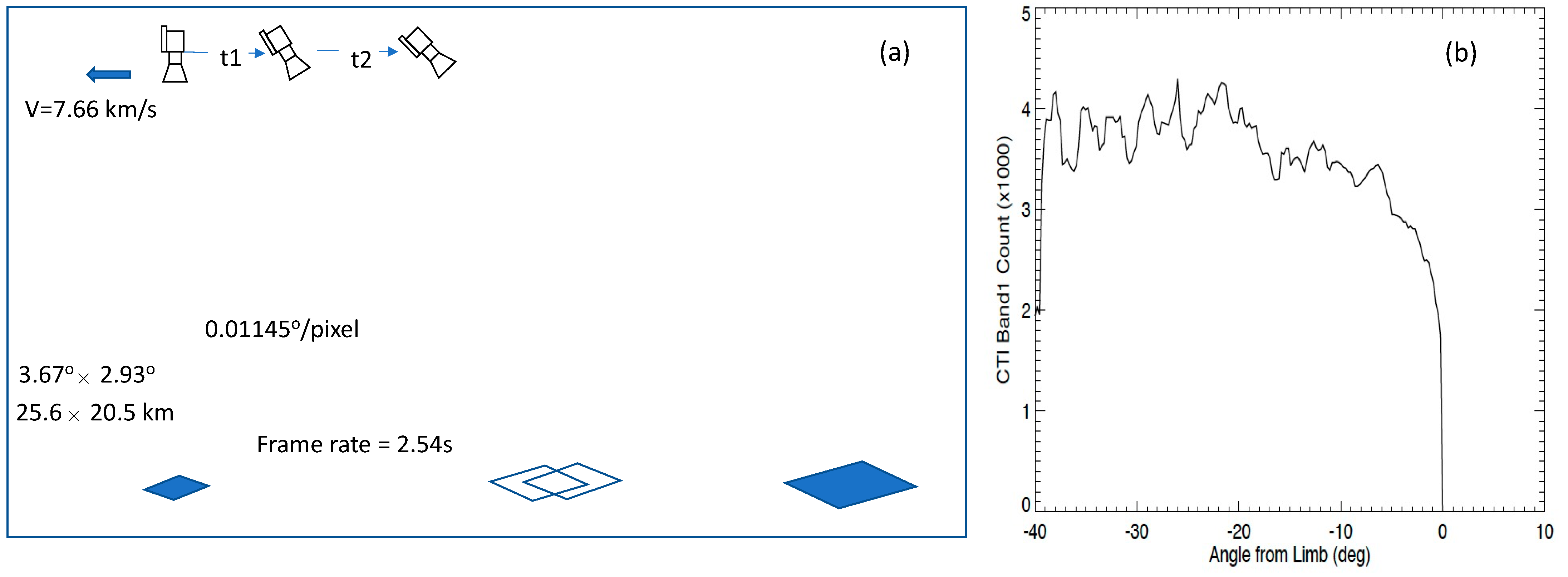
The ISS pitch-up/down operation provided a valuable opportunity for the CTI to profile the atmospheric limb radiation in the MWIR (midwave infrared) and LWIR (longwave infrared) bands. Although the pitch-up/down events were rare, the CTI acquired a few image sequences that demonstrated its capability and sensitivity of profiling limb radiances. The typical rate of ISS pitch-up/down is ~0.1°/s, which is much slower than the CTI frame rate. As a result, there was a stack of limb frames overlapped with each other in the pitch-up/down observations. The overlapped frames, each of which had a 3.67° × 2.93° field-of-view (FOV), allowed us to estimate the ISS pitch-up/down rate very accurately for each individual maneuver case. Figure 1 illustrates the scenario when the ISS undertook a pitch-up operation. During incoming (i.e., Russian) vehicle docking, the ISS often pitched up in the direction opposite to its flight velocity. The CTI camera moved from its nadir view to a slant view and eventually to limb and space views. Figure 1 shows the actual CTI band1 count measurements as the camera view angle moved towards the limb. The off-nadir CTI images during the pitch-up operation could have a large overlapped FOV with each other. At off-nadir pointing, the atmospheric pathlength also increased, which reduced the observed IR radiance. Because the atmospheric radiation made a significant contribution to the CTI radiance, and the atmosphere emits at a colder blackbody temperature than the surface, the increasing atmospheric pathlength tended to yield a colder brightness temperature or lower radiance. Known as the limb darkening effect, the decreasing count (or radiance) value towards the limb is evident in Figure 1b.
Figure 2 and 
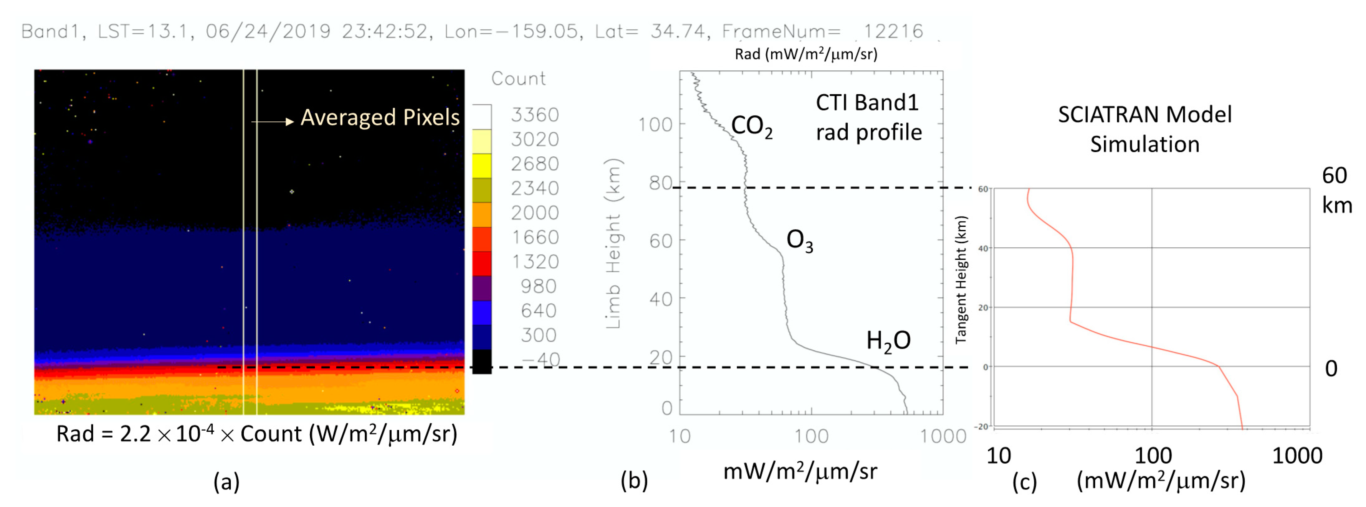
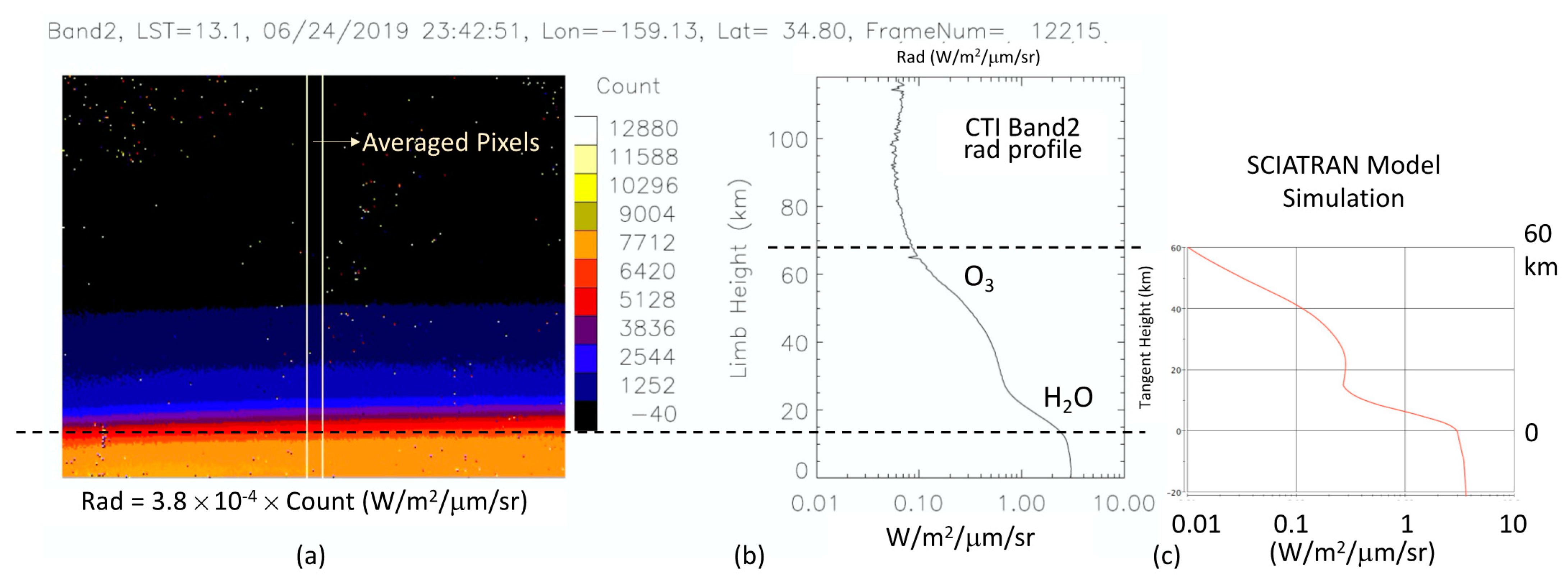
Figure 3 show a daytime frame of CTI band1 and band2 limb radiances from an ISS pitch-down operation on 24 June 2019. Each frame produced a limb view of 148 × 118 km (column × row), moving slowly at a rate of 2.54 s/frame with respect to the pitch-down maneuver. In this case, the ISS was pitching down in the CTI column direction, and each frame had a vertical span of 118 km (256 pixels) with a ~460 m resolution in limb height. The CTI frame rate allowed a continuous observation of atmospheric limb emissions with a stack of overlapping images. In addition, one can average the CTI column measurements that had the same vertical resolution to improve the signal-to-noise ratio (SNR) of the limb radiance measurement. The limb radiance profiles in Figure 2b and 
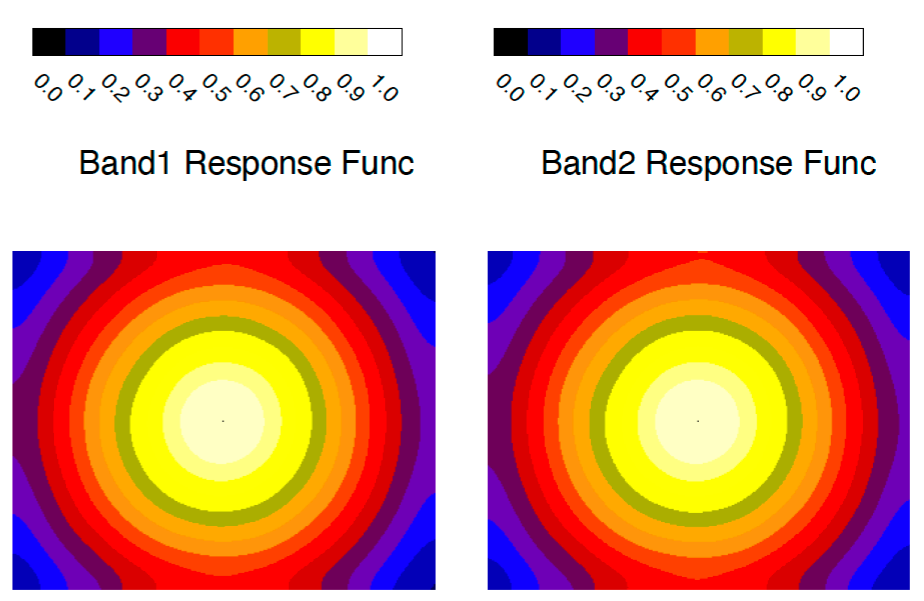
Figure 3b are the averages of 10-pixel columns in the middle of the frame. Because of the vignetting effect (Appendix A), the middle-frame pixels had a better sensitivity to atmospheric emissions than those on the edge. Especially for very weak limb radiances, the highest SNR pixels from the middle of the frame were selected to characterize the radiance profile at high altitudes.
Atmospheric O3 and H2O were the dominant sources of the limb radiance seen by CTI bands, and additional contributions from CO2 were evident in the band1 radiance at the mesospheric altitudes. Because of the relatively wide spectral bandwidth of the CTI bands, the emissions from these major atmospheric gases were always present in the CTI limb measurements, and atmospheric H2O became increasingly important at the lower tangent heights.
The observed limb radiances compared reasonably well with simulations from SCIATRAN, a radiative transfer model for the terrestrial atmosphere and ocean in the spectral range of 0.18–40 μm. SCIATRAN was developed for the SCanning Imaging Absorption spectroMeter for Atmospheric CartograpHY (SCIAMACHY) instrument and later generalized to include multiple scattering processes, polarization, thermal emission, and ocean–atmosphere coupling [14]. The software is now capable of modeling unpolarized (scalar) spectral and angular distributions of the intensity or the polarimetric Stokes vector of the transmitted, scattered, reflected, and emitted radiation, assuming either a plane-parallel or a spherical atmosphere. SCIATRAN simulations for CTI were performed under the spherical atmosphere, taking inputs from the NRLMSISE-00 (Naval Research Laboratory Mass Spectrometer and Incoherent Scatter Radar Exosphere-2000) empirical model [15]. The limb radiance spectra at 0.2–20 μm were computed for each tangent height up to 60 km and convolved with the CTI spectral functions to produce modeled CTI band1 and band2 radiances. The simulated CTI limb radiances did not exactly match the observed profile, because the input H2O, O3, and CO2 profiles obtained from NRLMSISE-00 may not have been accurate enough to represent the real atmospheric state at the time when the observation was made. However, the simulation captured the basic features seen by the CTI bands, and the radiance values were in general agreement with the calibration based on VIIRS (Appendix B).

3.2. Gravity Waves in CTI Limb Radiances

Atmospheric gravity waves (GWs) are the disturbances generated in a stably stratified layer where the density equilibrium is balanced between gravity and buoyancy forces. Often excited from the troposphere, GWs with horizontal scales of <1000 km can propagate upwards into the stratosphere and above while growing in amplitude. Both limb and nadir sounding techniques have been employed for GW observations [8]. Limb techniques tend to yield better vertical resolution, whereas nadir observations have better horizontal resolution. However, most limb sounding instruments produce only a vertical scan (1D), which misses the two-dimensional (2D) perspective of propagating gravity waves in the atmosphere.
The high-resolution CTI limb view during the ISS pitch-up/down operation provided a new, attractive capability for 2D images of GW structures. 
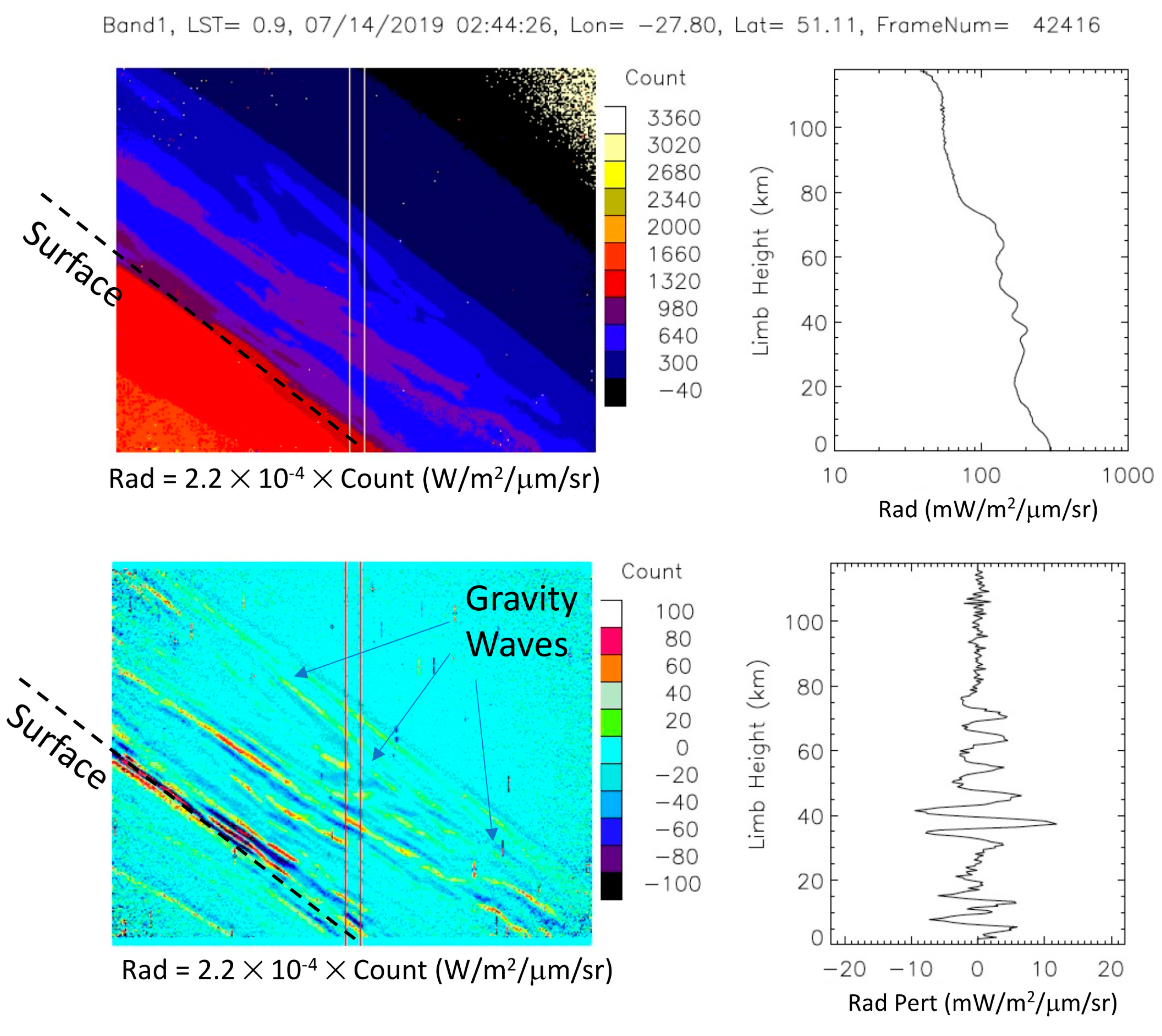
Figure 4 shows an example of GW-modulated limb radiances in the CTI images. Because the thermal emissions from atmospheric O3 and H2O layers are proportional to the density of these gases, the density disturbances induced by GWs manifest themselves as limb radiance fluctuations. In fact, the limb radiance fluctuations can be seen in the raw CTI data in the top panels of Figure 4. By removing the background limb radiances, which were from a 11-pixel running mean of each detector column, these wave perturbations became more pronounced. One can readily see a tilted structure with respect to the limb horizon with an apparent vertical wavelength (~10 km). As illustrated in the previous CTI limb case, the limb height was not the tangent height, but it could be used to infer the tangent height by subtracting the surface tangent height estimated using the modeled limb radiance profile shape (e.g., Figure 2 and Figure 3).
It requires more quantitative analysis to properly interpret the observed GW features in terms of GW horizontal and vertical wavelengths, because the CTI bands were broadband channels with contributions from both optically thin and optically thick emissions of atmospheric gases. Horizontal and vertical wavelengths are valuable GW properties to understand the origination, dissipation, and breakdown of GWs in the atmosphere [16]. If the limb radiance is dominated by optically thin emissions, it is proportional to atmospheric gas concentration. In this case, the observed GW structures would indicate waves in horizontal and vertical propagation, as the gas concentration profile is modulated by GWs. A typical example of using the optically thin technique for GW observations can be found in [17], in which vertical wave perturbations were extracted from each limb profile and consecutive perturbation profiles were tracked along the satellite track to find horizontal wave perturbations. In the case where the limb radiance is dominated by optically thick emissions, these radiances are essentially proportional to the temperature of the blackbody emission from a fixed atmospheric layer, which can occur at the bottom of limb radiance profile as seen in Figure 2 and Figure 3. In this case, the observed GW structures would mostly reflect the horizontal temperature fluctuations induced by waves [18]. Examples include satellite slant-view MWIR imagery [19] and cross-track LWIR sounding radiances [20]. Using airborne IR limb imagery from multiple flight paths and viewing angles, Krisch et al. [21] observed a tilted wave structure in limb temperature perturbations and was able to reconstruct the 3D GW structure with a tomographic retrieval. Here, the CTI demonstrated another case from space in which propagating GWs in the lower and middle atmosphere could be detected from high-resolution 2D limb IR imagery.
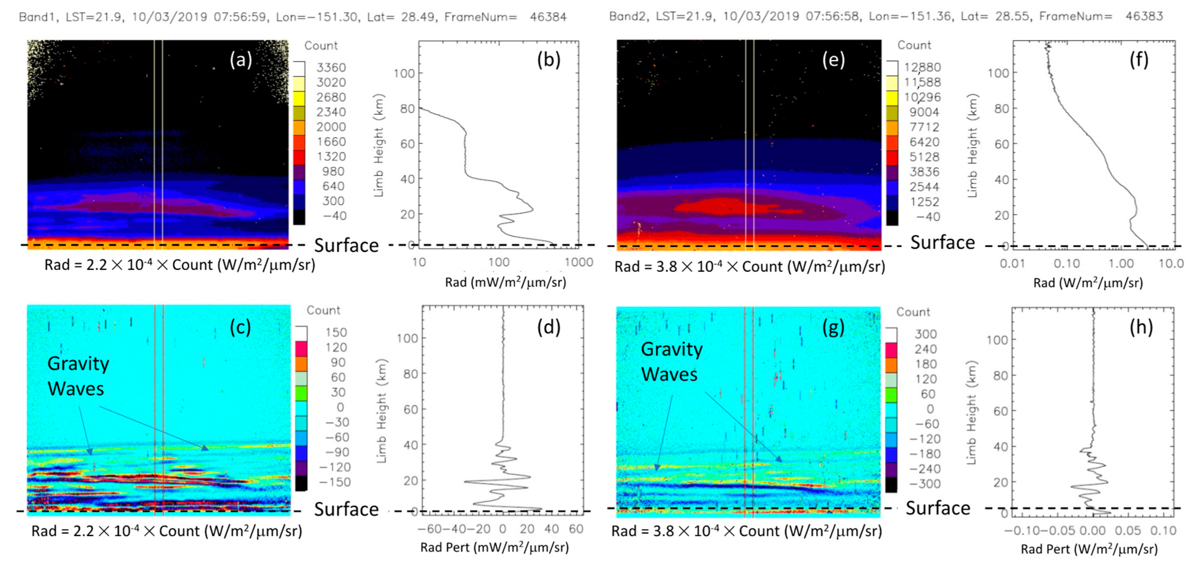
Not all CTI limb observations had a clear GW feature, but Figure 5 captures another GW event in both band1 and band2 images. In this case, there was a distinct nighttime O3 layer and the presence of GWs in the stratosphere. Despite very different radiance intensities, both bands revealed a similar wave structure in this FOV. GW-modulated radiance perturbations had clear tilted structures at 20–40 km limb heights with an apparent vertical wavelength of <10 km and a horizontal wavelength < 50 km. Like the case in Figure 4 for band1, the waves in the lower stratosphere were tilted in a different direction than those in the upper stratosphere. These small-scale GWs, unresolved by global numerical weather prediction and climate model simulations, have been a great challenge in new model development because their momentum fluxes need to be taken into account through parameterization schemes in order to correctly determine atmospheric circulation and thermal structures [22]. High-resolution thermal imagers such as CTI can provide the needed GW observations to guide future global model developments.
From the perturbation profiles in Figure 4 and Figure 5, we estimated that the single-pixel CTI radiance uncertainties (1-sigma) were ~4 and ~5 mW/m2/μm/sr for band1 and band2, respectively. The estimation was based on the random radiance fluctuations in the deep-space portion of the images, such as the high-altitude measurements in Figure 4 and Figure 5. For significant GW detection, radiance oscillations need to have an amplitude 2-sigma greater than the radiance random error. Because of the high sensitivity and stability of the CTI SLS detector, these weak GW-induced limb radiance signals were detectable. Furthermore, the CTI radiance sensitivity, if converted to the minimum detectable brightness temperature using the look-up table in Appendix B, would be ~0.1 K at 300 K, ~0.2 K at 273 K, and ~0.5 K at 250 K for band1; and ~0.04 K at 300 K, ~0.07 K at 273 K, and ~0.1 K at 250 K for band2.

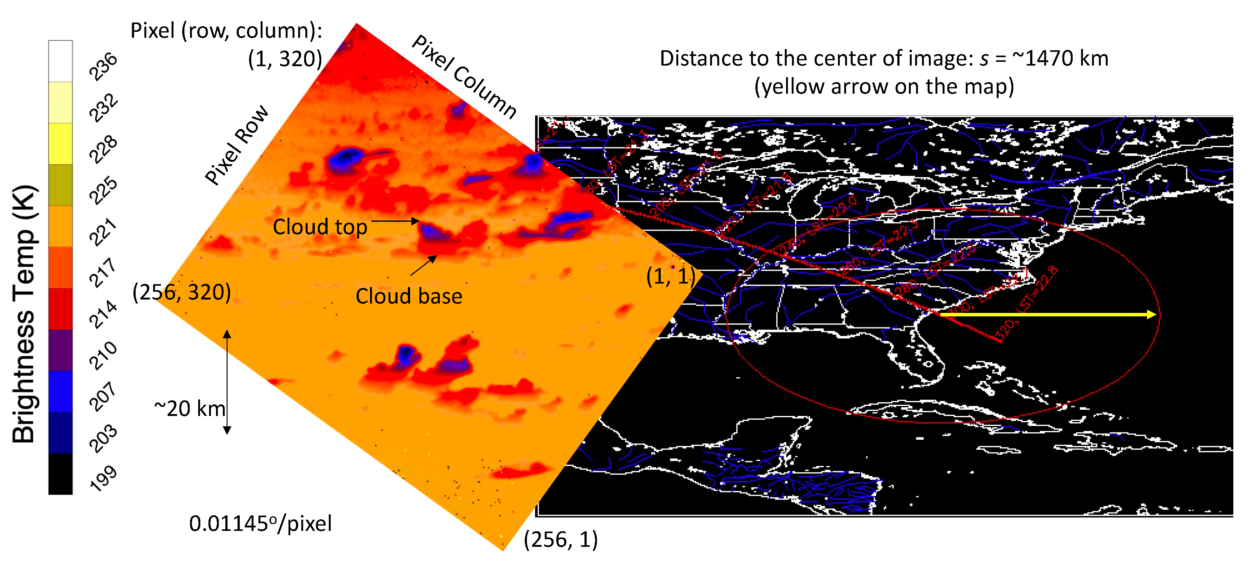
3.3. Profiling Clouds from the Slant View

High-resolution CTI imagery provides the capability of profiling cloud tower temperatures from a slant viewing angle. As in the limb geometry, the slant-view geometry observes cloud towers from the side, and the pixel resolution turns into a vertical resolution for cloud profiles. In other words, instead of measuring cloud top temperature, CTI images at an oblique angle measure the vertical profile of cloud temperature. As shown in Figure 6, this technique works particularly well for isolated cloud towers where there is little overlap between clouds. This frame from the ISS pitch-up operation had an ~80° incident angle or a distance of ~1470 km between the ISS and the center scene of the image. This distance suggests that a pixel had the vertical resolution of ~290 m from the side view of a cloud, which is comparable to the CloudSat radar resolution [23].
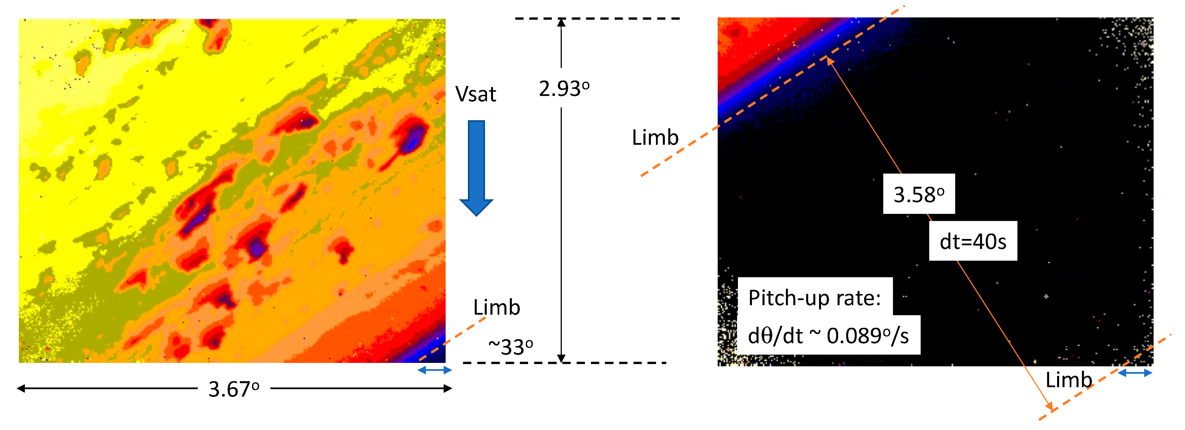
We estimated the rate of ISS pitch-up/down using a series of frames, as shown in Figure 7, when the Earth’s limb swept through the CTI images. In the case on 1 August 2019, the pitch-up plane was ~33° with respect to flight direction, such that the limb was not in parallel to either the image’s row or column orientation. From the estimated pitch-up rate (0.089°/s), we could track back the pointing angle of each frame with respect to the angle of the limb to determine the distance between the ISS and the imaged scene. From the distance, the vertical resolution of individual pixels could be calculated. As seen in Figure 7, the near-side (closer to nadir) cloud towers had apparent heights that were taller than those of the far-side (closer to limb) towers, largely because of the differences in pixel vertical resolution from the distance effect.
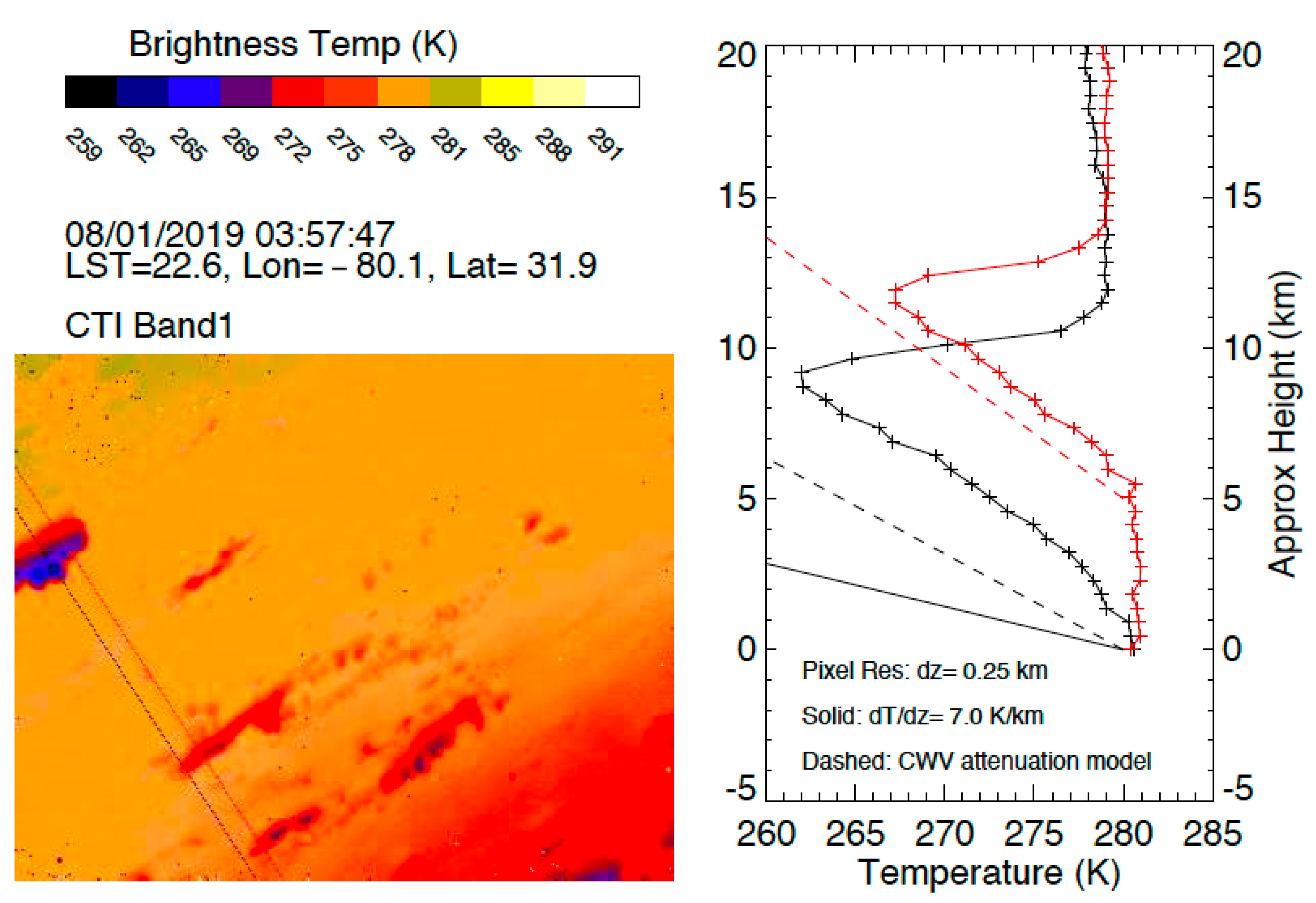
A nighttime frame with isolated cloud towers on the near side of the CTI band image acquired on 1 August 2019 was particularly interesting, showing a clear vertical distribution of cloud temperature (Figure 8). CTI had a vertical resolution of ~250 m for this cloud observation, and the two vertical cross sections cut through clouds show a temperature of 281 K at the cloud bottom, 263 K at the top for a taller tower, and 267 K at the top for a shorter tower. The gradually decreasing cloud temperature with height is expected for a colder atmosphere/cloud at higher altitudes. Such a side-view cloud temperature profile was reported from an airborne thermal imager with the potential to profile cloud thermodynamic phase and microphysical properties [24]. Because of the high-resolution of CTI imagery, here we showed that profiling clouds from a side-viewing geometry could be achieved from space.
A more quantitative understanding of the vertical gradient of CTI cloud temperature profiles requires consideration of radiative transfer of thermal emissions from clouds and the atmosphere. Because atmospheric column water vapor (CWV) between clouds and the CTI can act to attenuate the cloud emission, the observed cloud vertical temperature profiles did not follow the atmospheric temperature lapse rate (e.g., ~7 K/km). This effect can be quantitatively described by a simple model as follows:
T B ( z ) = α × T CWV + ( 1 α ) × T c l d ( z )
where T B (z) is the apparent brightness temperature profile observed by CTI, T CWV is the CWV temperature, T c l d (z) is the cloud temperature profile, α is the CWV emission coefficient, and (1 −   α ) is the CWV attenuation on cloud emission. In the presence of CWV attenuation, the observed cloud temperature profiles would appear as a shallow slope. As shown in Figure 8, with α = 0.55 and T CWV = 280 K, the 7 K/km lapse rate would appear as the dashed line for the cloud closer to CTI (black curve), whereas the slope for the cloud farther away (red curve) would be shallower, as expected for more CWV attenuation ( α = 0.67 and T CWV = 280 K). Using a larger CWV value, the attenuated slope would match the observed cloud temperature profile.

3.4. Planetary Boundary Layer (PBL) Clouds

In addition to the new looks at limb and slant views, the high-resolution high-sensitivity imaging from the CTI has potential applications for remote sensing of clouds in the PBL. Because PBL clouds are close to the surface, they have relatively poorer contrast in IR images than in visible images, which makes it more challenging to observe PBL clouds at MWIR and LWIR wavelengths. On the other hand, observations of PBL clouds during both daytime and nighttime are highly desirable in order to study the diurnal cycle of these clouds.
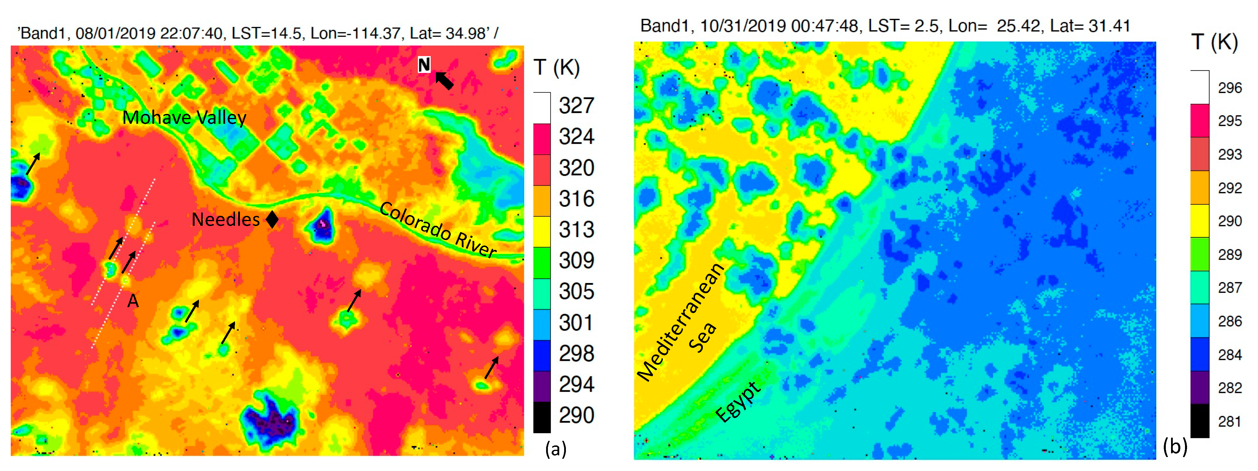
The two cases in Figure 9 show good contrast between PBL clouds and the surface background emission in CTI daytime and nighttime images. In the daytime case, broken PBL clouds during summer over the Mojave Desert were evident as a colder object against the hot surface. The surface temperature in Death Valley (Stovepipe Wells, California) on this day had reportedly reached an hourly maximum of 320 K, which was consistent with the CTI temperature estimated from the VIIRS calibration. Among other deserts (e.g., the Lut Desert in Iran or the Sonoran Desert in Mexica), Death Valley is one of the hottest places in the world in terms of land surface temperature (LST) [
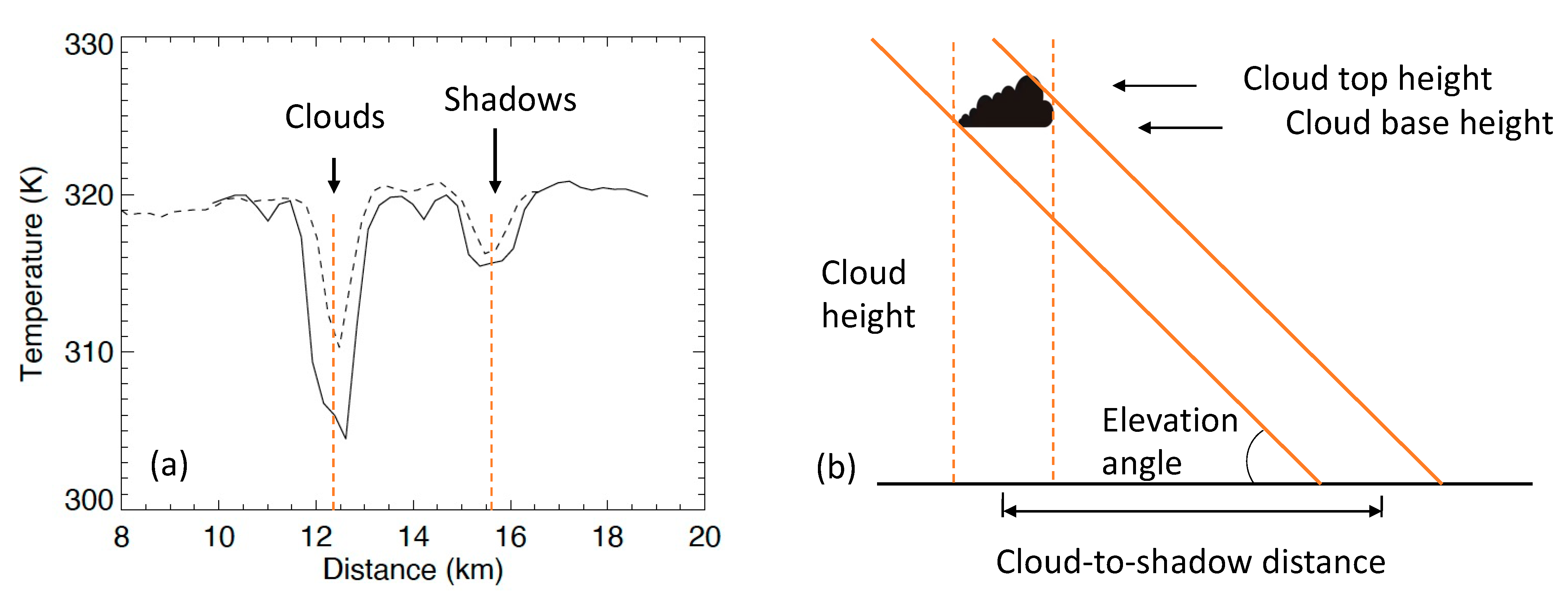
25]. In addition to cloud and surface temperatures, the cloud shadow can also be seen in the CTI band1 image, showing a temperature slightly cooler than that of the surface but a warmer than that of the clouds.
The cloud–shadow pairs, separated roughly by the same distance, indicated that these PBL clouds had the same cloud base height (CBH). Figure 10 presents a rough estimate of CBH from the cloud-to-shadow separation using a simple geometric calculation. Because the shadow reflects the horizontal extent of a cloud, which is largely determined by the cloud base, we interpreted the cloud height derived from the cloud shadow as the CBH. The CBH over deserts is a good measure of the convective condensation level (CCL) at which condensation begins to occur, which is the stability property of the atmosphere and has impacts on potential development of severe thunderstorms. From the cloud-to-shadow distance and the Sun’s elevation angle, we found that these clouds had a CBH of ~4.9 km. This high CBH was not surprising for a hot desert environment, given that a reported mean CBH was >2.5 km over the Mojave Desert during the summer [26].
PBL cloud detection poses a greater challenge for passive IR imaging from space because of weak contrast between clouds and background surface emissions, and visible imagery is often brought to assist in cloud discrimination. At night, cloud detection has to rely solely on the thermal contrast in the IR imagery. Small-scale cloud and surface inhomogeneity constitute a major obstacle for IR imagers with coarser resolution to generate a significant cloud–surface contrast because of the blurring effect. Thus, the combined high resolution and high sensitivity of CTI thermal imagery can provide a significantly enhanced contrast between PBL clouds and background surface emissions. Figure 9b illustrates a scene of nighttime PBL clouds above different surface backgrounds over the coast of Egypt. Since the ocean temperature is often warmer than near-surface air at night, PBL clouds can be readily classified as a cold feature. Because the CTI band1 had an excellent sensitivity (0.1–0.2 K at 273–300 K), these nighttime clouds could be reliably detected from a weak surface–cloud contrast. This capability is evident in Figure 9b, where the LST gradient reduced the cloud–surface contrast over Egypt from the bottom of the image to the top. In this nighttime land case, PBL clouds were still visible at LST ~286 K, which was ~1 K warmer than the cloud temperature.
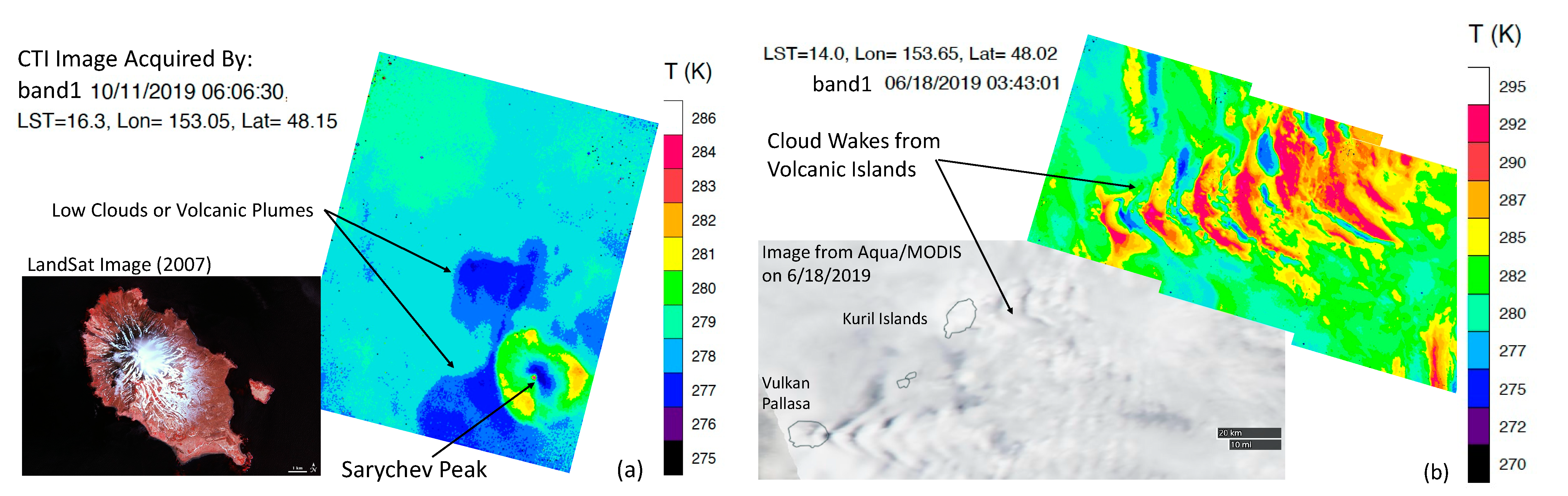
The CTI made a number of high-resolution observations over active volcanos and their surrounding environments. As shown in Figure 11a, the CTI took a snapshot of Sarychev Peak on 11 October 2019, showing low clouds or volcanic ash plumes surrounding the volcano. Sarychev Peak is an active volcano that had a strong eruption in June 2009. Although there was no major eruption at the time of the CTI flight on ISS, small thermal anomalies were reported in infrared imagery during June–October 2019 [27]. The volcanic plumes or plume-generated low clouds were quite distinct, with temperatures colder than the ocean, exhibiting a shape panning out from the volcano. On the other hand, volcanic islands can act as an obstacle to atmospheric flow, generating cloud wakes downstream. In nearly coincident observations, both Aqua/MODIS (Moderate Resolution Imaging Spectroradiometer) visible and CTI MWIR channels captured a cloud wake structure from the Kuril Islands (46°30′N 151°30′E) on 18 June 2019 (Figure 11b). The cloud wakes were somewhat blurry in the MODIS image because of its 250 m pixel resolution, but they were more structured in the CTI image. In summary, the high-resolution, high-sensitivity CTI imagery showed additional capabilities for isolating low-level clouds.

3.5. Global Cloudiness and Diurnal Variations

The CTI on the ISS had nearly continuous operation between 2 May and 8 November 2019, allowing us to develop nearly global statistics of atmospheric and surface temperatures and their diurnal variations at latitudes covered by the ISS. Unlike the ECOsystem Spaceborne Thermal Radiometer Experiment on Space Station (ECOSTRESS) mission, which used an LWIR imager to measure land evapotranspiration for targeted regions [28], the CTI made continuous observations of clouds and surfaces with a more uniform distribution in latitude and longitude under the ISS coverage. Therefore, the CTI data are particularly valuable to develop cloud temperature statistics for studying the LW radiation and their local-time variations.
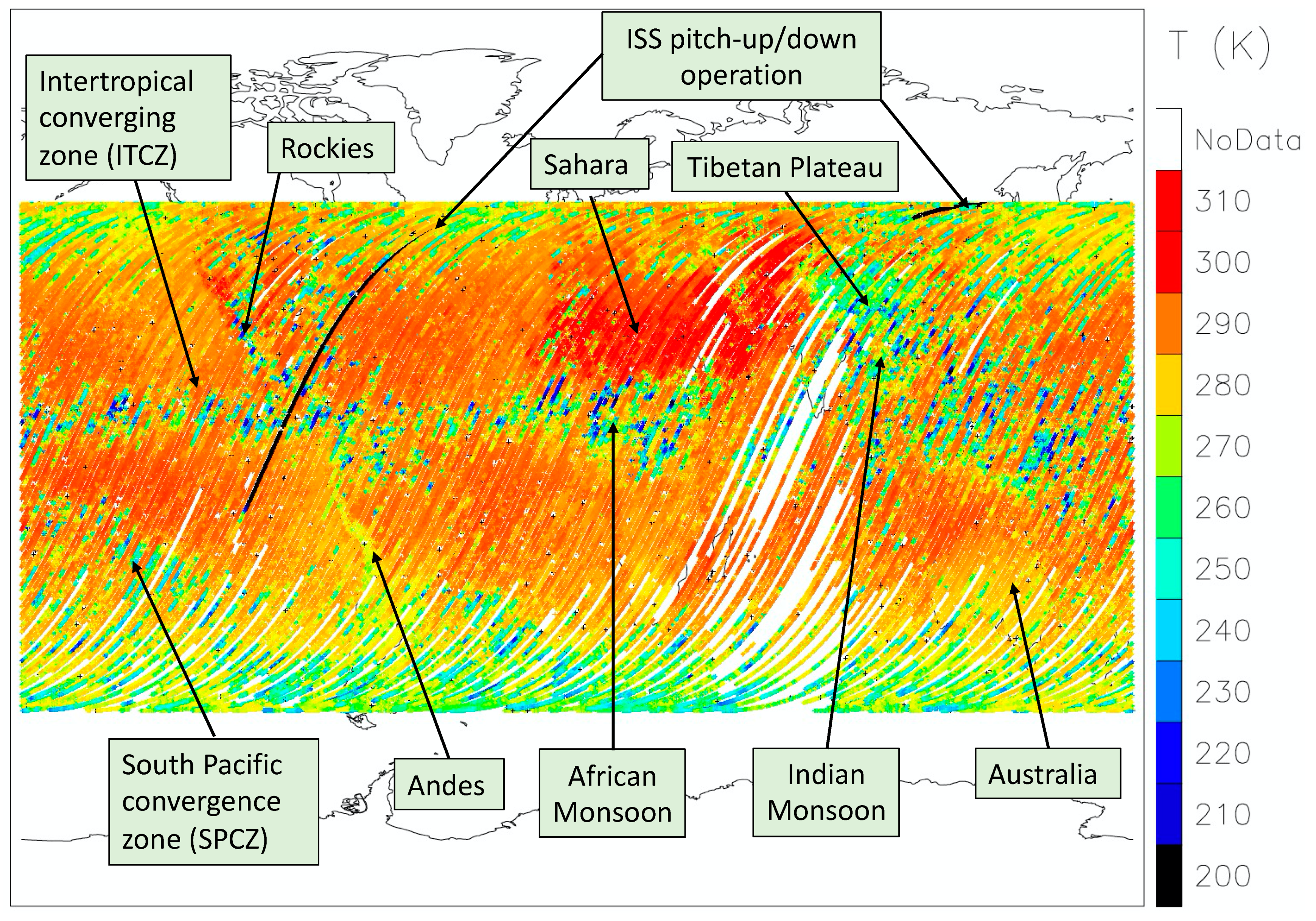
To illustrate this CTI global sampling, we show in Figure 12 a nighttime map of CTI band1 brightness temperatures from July 2019. The map reveals several well-known cold (e.g., deep convective clouds over ITCZ and SPCZ, Indian and African Monsoons, Tibetan Plateau, Rockies, and Andes) and warm (e.g., Sahara, Mideast) features. At MWIR wavelengths, upper-tropospheric clouds emitted at a colder temperature than the surface and thus manifested themselves as features with cold temperatures. These clouds were often associated with deep convection in the tropics and subtropics, as seen in Figure 12. In addition, high mountains also emitted at a cold temperature, whereas clear-sky oceans and the oceans with low clouds tended to have high emission temperatures around 290 K at low latitudes. The Sahara and the Middle East were the warmest places in July at night.
Cloud-induced radiance/temperature variations are perhaps better illustrated using a probability density function (PDF) in which clouds manifest as a cold tail of the temperature distribution. The bin size of the band2 brightness temperature PDF was 1 K in this analysis. To compare the statistics of cloud and surface variations from different locations and times, we normalized the PDF by dividing it by the total number of samples in each bin. In other words, the sum of the normalized PDF was always unity. The normalized PDF was derived for each latitude (5°) and local time (2-hourly) bin from the data acquired in June–August (JJA) 2019.
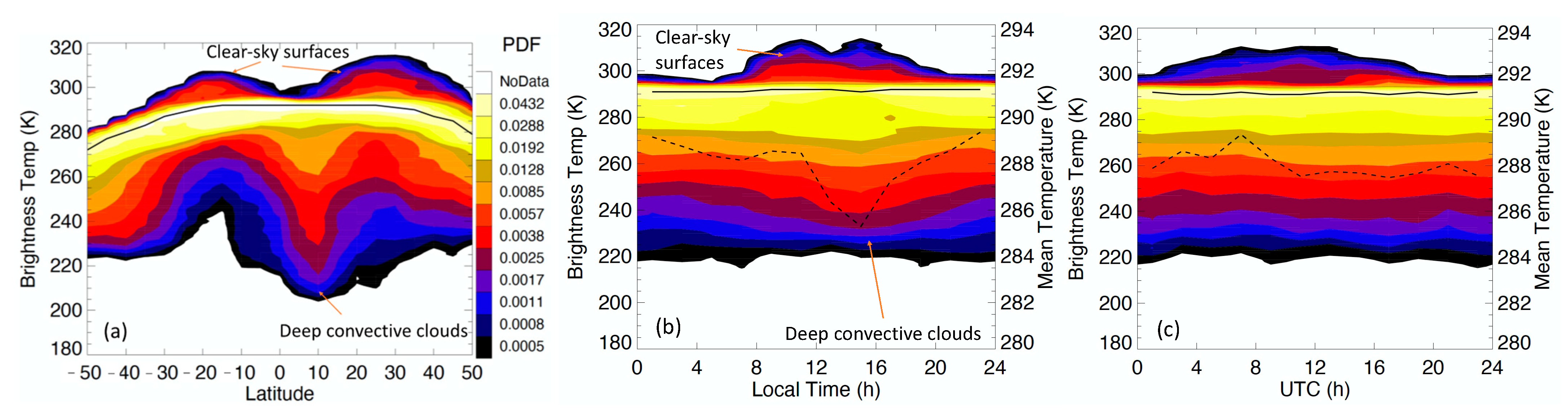
The zonal mean PDF of CTI band2 brightness temperatures shown in 
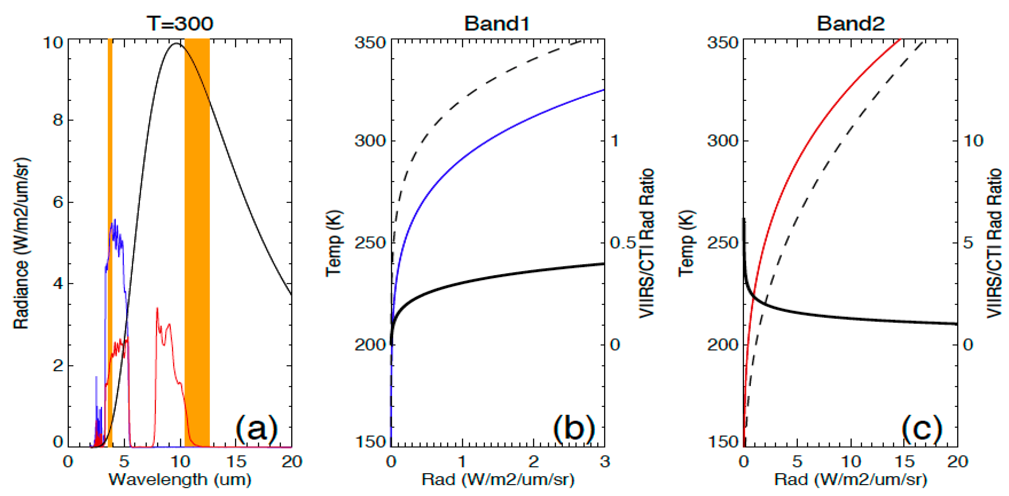
Figure 13a revealed several key atmospheric and surface features. Tropical deep convective clouds showed an enhanced PDF at cold temperatures, which resulted from the uprising branch of the Hadley circulation. This branch was flanked by two depressed PDFs in the subtropical latitudes, known as the subsiding regions of the Hadley circulation, which bring cold and dry air down to the lower troposphere. On the warm side of the subtropical PDFs, the enhanced distributions were primarily from hot daytime land surfaces. These warm features were from subtropical arid regions wherein surface temperatures varied strongly with the solar heating during daytime hours. At midlatitudes, clouds from baroclinic storms and extratropical cyclones were also evident as an enhanced PDF at cold temperatures. For the JJA months, the temperatures at the PDF peak were nearly constant (~292 K) at latitudes between 20°S and 30°N, as they were primarily determined by global ocean and moist atmospheric emissions. Although the CTI filter blocked the water vapor emission at 5–7 μm, there was still a significant amount of column water vapor contribution in the CTI band2 radiance, as seen in Figure 3.
Because the ISS orbit has a nodal precession rate of ~6°/day, the CTI band2 sampling during JJA provided useful observations of the diurnal variation of Earth’s outgoing LWIR radiation. It takes roughly 60 days to sample the full diurnal cycle from ISS with a single node (i.e., the ascending or descending orbits only). However, with two nodes (i.e., both ascending and descending orbits), this sampling period can be shortened to ~30 days. From the ISS orbit, the CTI sampling provided two solar local times at the equator on a given day from the ascending and descending nodes, but the sampling reduced to one local time at the turning latitudes (i.e., 51.6°N/°S). In other words, we were able to obtain a full diurnal cycle with 30 days’ worth of CTI data at the equator but would need 60 days of data at the 51.6°N/°S latitudes. Seasonal cloud and surface variations may contaminate the diurnal result when a longer period of observations is used. Previous studies on cloud diurnal cycles from the ISS included a submillimeter wave radiometer [29] and a lidar [30].
The diurnal cycle of CTI brightness temperatures can be evaluated with respect to two reference times: solar local time (SLT) and coordinated universal time (UTC). SLT diagnostics focus on local solar heating and thermodynamic responses to the heating at a process level, whereas UTC diagnostics address the energy budget at a specific time from a global perspective. As shown in Figure 13b for the local time dependence of temperature PDF, the mean CTI band2 temperature from 50°S–50°N latitudes was highly correlated with the occurrence of deep convective clouds: the greater the high-cloud cover, the lower the mean temperature. On average, the lowest mean temperature occurred at ~3 h after noon, although hot surfaces (T > 300 K) peaked around noon. With respective to UTC, the PDFs of CTI band2 temperature showed less variability at cold (cloud) temperatures, except at temperatures warmer than 295 K (mostly from land surfaces). The mean temperature showed only small variations with a peak at UTC = 08Z.
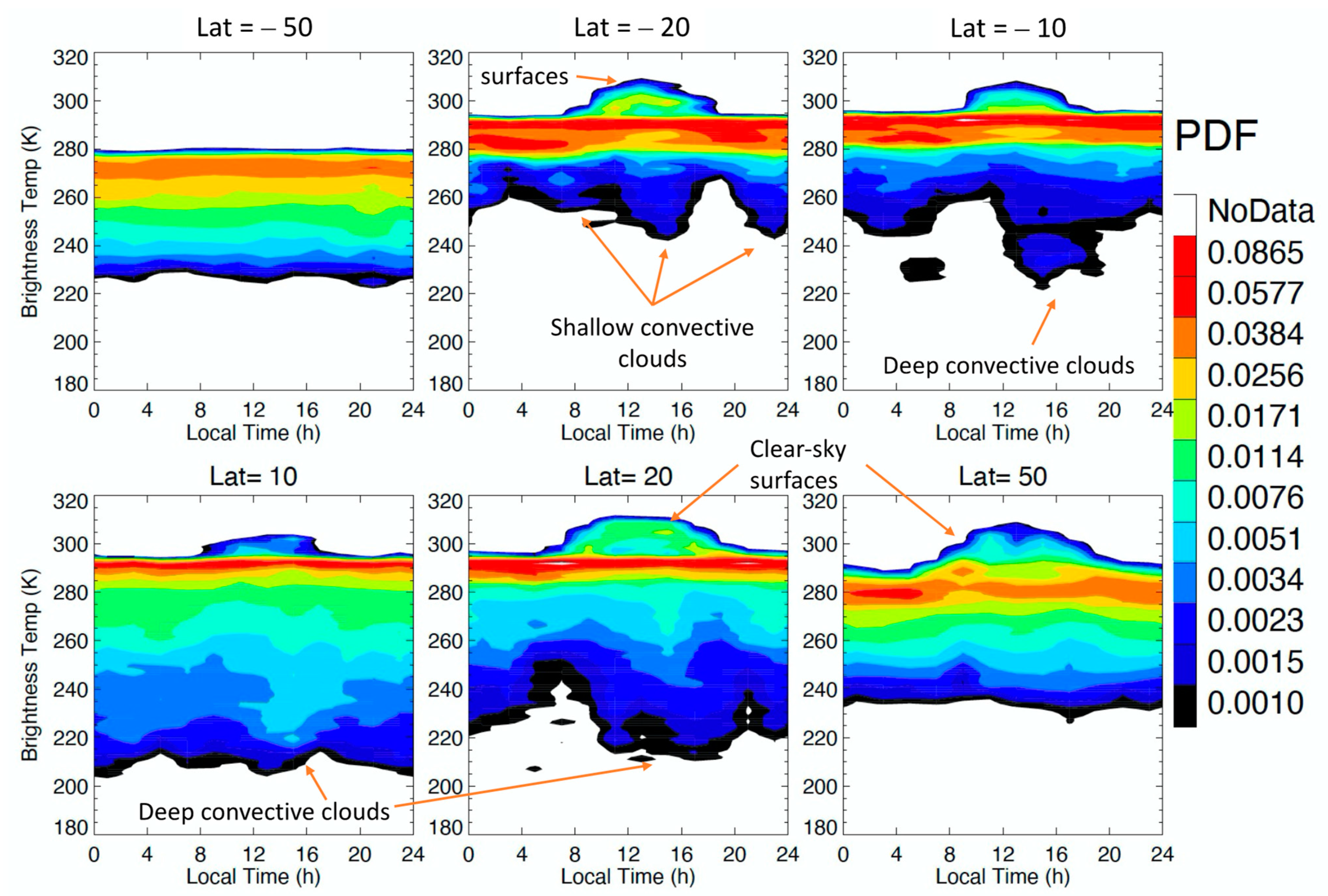
The PDFs of local time variations were more pronounced at individual latitude bins, as both solar surface heating and deep convective cloud developments are the driving processes at a regional scale (Figure 14). The PDF diurnal variation at temperatures warmer than 295 K was a salient feature at most latitudes except 50°S. This temperature range captured the variations of the land surface temperature, which covaried with solar-angle-dependent heating. During JJA, differences in day length were clearly evident between the PDFs at 20°S and 20°N. At the colder temperatures, cloud-induced PDFs exhibited different local-time variations, ranging from a 4-hourly modulation at 20°S, to a 12-hourly one at 10°S and 20°N, to a 24-hourly one at 10°N. These latitude-binned diurnal variations contained a mixed signal from clouds over ocean and from land. Clouds over land tended to have a strong 24-h variation with a peak in the late afternoon, while tropical oceanic clouds tended to have a semidiurnal variation [31,32,33]. The PDFs from deep convective clouds at 10°N also revealed a short (~3 h) lifetime of deep convective clouds, with the peak time in the early afternoon. The diurnal variation at 50°S was relatively weak, as most longitudes were covered by the Southern Ocean.
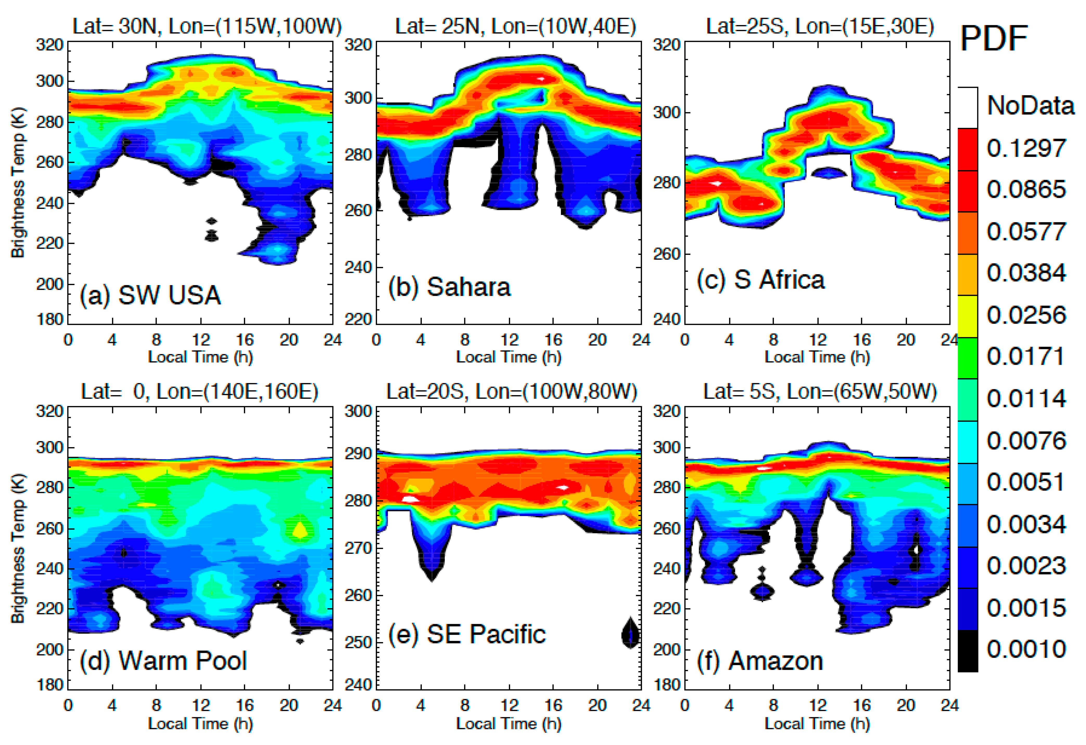
The PDFs of local-time variation for smaller regions provided a better understanding of the processes that drive diurnal differences. In the southwest United States (Figure 15a), deep convective clouds in late afternoon were the dominant feature in the PDF, as JJA is the monsoon season, and late-afternoon storms are driven by strong solar heating over land. Over the Sahara (Figure 15b), JJA is its wet season, with multiple distinct periods of rainfall, but the convective clouds were not as deep as those over the southwest United States. By contrast, surface temperature variation dominated the diurnal cycle in southern Africa (Figure 15c), where there are very few clouds during the dry season. In the western Pacific warm pool (Figure 15d), the PDF of CTI temperatures was consistent with the active period of cloud-top temperature PDFs from geostationary satellite IR sensors [31]. In the Southeast Pacific, where stratocumulus clouds prevail (Figure 15e), the CTI temperatures were mostly bounded between 278 and 290 K as the marine PBL clouds were capped by a 10–12 K temperature inversion [34]. During the dry season over the Amazon rainforest (Figure 15f), the diurnal range in surface temperatures was small, based on surface cooling from evapotranspiration. Convective rainfall could occur at multiple times through the day. In other Amazon regions, deforestation may change the amount of rainfall [35] and the length of the dry season [36].
We note that the decision to evaluate three months of data from CTI to improve the sampling for all local times and latitude bins (Figure 14 and Figure 15) may have led to some confounding effects from seasonal variability in the diurnal cycle. If the diurnal cycle was a repeatable pattern during June–July, the CTI observations would represent such diurnal variability. However, if the diurnal cycle had a significant seasonal modulation, the aggregated local-time variation would include this variability. Thus, the regional results shown in Figure 15 should be viewed as a gross diurnal variation because of the limited number of samples acquired by CTI.
In summary, the stable detector performance and good radiometric sensitivity from CTI allowed consistent calibration for several months even when the ISS experienced very different beta angles and thermal environments. As a result, the CTI band2 calibrated brightness temperatures provided a reasonable diurnal variation of surface and cloud temperatures with respect to local time during JJA in 2019.

4. Conclusions

In this paper, we presented a number of interesting atmospheric observations from the CTI on the ISS during its operation period between February and November 2019. While the CTI was designed as a free-running radiometer/imager to demonstrate a new SLS detector technology, we successfully developed a flat-field correction algorithm and made radiometric calibration for the two spectral bands using collocated SNPP/VIIRS data. The calibrated CTI radiance and brightness temperature data are scientifically useful for atmospheric and surface studies, including limb sounding, gravity waves (GWs), convective and boundary-layer clouds, volcanic plumes, and the diurnal variation of surface and cloud temperatures.
The combined high-resolution and high-sensitivity qualities of CTI imagery provided a new look at these atmospheric phenomena. Although there were a limited number of limb-viewing opportunities from the ISS pitch-up/down operation, the high-resolution CTI imagery was able to detect several small-scale structures in the limb radiance induced by atmospheric GWs. These slantwise views of tilted GW structures were not observed previously by operational limb sounders because of either coarser resolution or a single limb-scan beam. Thus, CTI-like imaging sounding can provide a higher-resolution and wider look at limb radiances for atmosphere GW studies. The limb radiance profiles observed by the CTI were broadband IR emissions, reflecting a collective contribution from the major atmospheric trace gases (e.g., H2O, O3, CO2). For future science applications, a CTI-like instrument needs to incorporate narrow-band filters or a spectrometer in these bands to allow the retrieval of species abundance profile from different tangent heights.
The high-resolution CTI measurements also benefited cloud detection and characterization. Not only could the CTI better isolate boundary-layer clouds with a finer vertical resolution, but it demonstrated the capability of profiling cloud tower temperatures from a slant view. We showed that the high-sensitivity CTI imagery helped to improve cloud detection by resolving the small-scale thermal contrast between cloud and surface emissions. In the case in which clouds were very close to the surface, and both had a highly inhomogeneous distribution, the combined high-resolution and high-sensitivity imaging helped to overcome the poor contrast induced by the smearing of coarse-resolution sensors.
The CTI band2 brightness temperatures revealed useful statistics of the diurnal variations of land surface and cloud development in terms of the normalized PDF. The realism of the observed diurnal variations confirmed the CTI SLS detector’s stability and its radiometric sensitivity. These properties play a key role in developing robust calibration algorithms for a free-running radiometer without onboard calibration sources. The ISS/CTI made nearly continuous observations of the Earth during May–October 2019. Because of the ISS’s orbital precession, the near-global coverage from the CTI will be particularly valuable for characterizing the tropical cloud diurnal variations in a future study.
The compact, low-power design of the CTI instrument will significantly reduce the size, weight, power, and cost (SWaP-C) of future IR imaging and remote sensing of the Earth. A constellation of CTI-like instruments on a SmallSat/CubeSat will be affordable for achieving the dense spatiotemporal sampling needed by science applications. A great effort has been made at the NASA Goddard Space Flight Center to raise the instrument technology readiness level (TRL) through the ISS/CTI experiment. Future CTI developments will aim to enhance the instrument’s capabilities to meet various measurement requirements from targeted science investigations. These enhancements will include a larger detector array, polarimetric capability, a front-end spectrometer, and/or narrow-band spectral filters. Combining a compact spectrometer and CTI detector technology will form a small limb-sounding instrument that will be capable of quantifying the abundance of O3, H2O, CH4, N2O, halogens, and polar stratospheric clouds (PSCs) in the upper troposphere and lower stratosphere (UT/LS).

Author Contributions

Conceptualization, D.L.W. and D.E.J.; methodology, D.L.W., D.E.J., M.D.J. and A.T.L.; software, D.L.W., D.E.J. and T.F.; validation, D.L.W., D.E.J., K.-K.C., J.A.L. and K.-M.K.; formal analysis, D.L.W., D.E.J. and K.-K.C.; investigation, D.L.W., D.E.J., K.-K.C., T.R.H., D.C.M., R.J.S. (Ross J. Salawitch), L.D.O. and J.G.; resources, D.L.W. and M.D.J.; writing, D.L.W. and D.E.J.; visualization, D.L.W.; supervision, M.D.J.; project administration, M.D.J.; funding acquisition, D.L.W., T.H. and R.J.S. (Robert J. Swap) All authors have read and agreed to the published version of the manuscript.

Funding

This study was funded by GSFC (Goddard Space Flight Center) Internal Research and Development Program (IRAD) from accounts 981698.01.02.51.03.10.07 and 981698.01.04.51.05.60.17.

Institutional Review Board Statement

Not applicable.

Informed Consent Statement

Not applicable.

Data Availability Statement

The CTI data are available upon request.

Acknowledgments

We would like to thank the ISS and the RRM3 project for hosting the CTI instrument and providing valuable observation time and data downlink.

Conflicts of Interest

The authors declare no conflict of interest.

Appendix A. Flat-Field Correction for CTI Digital Count Measurements

The CTI instrument did not have any onboard target for radiometric calibration. This appendix describes the algorithm for flat-field correction of CTI count measurements using deep-space views from ISS pitch-up/down maneuver operations. Because temperature variations in the CTI optics can affect the background count, an empirical frame-by-frame algorithm was developed to account for this temperature variability using the corner pixel measurements and the instrument response function.

Appendix A.1. A Conceptual Model of CTI Vignetting Optics

The CTI telescope and optics were described by Jhabvala et al. [1] (p. 5434). A conceptual optical schematic is shown in Figure A1, which includes the cold stop, window, spectral filter, and lens. An input baffle on the front of the telescope was used to minimize glint from exterior surfaces. The telescope and optics were divided into two temperature zones, with the detector and the cold stop in a cryogenic environment (<83 K), and the window, the filter, the lens and the baffle in a thermally stabilized ambient environment, which can vary considerably during each orbit.
Figure A1. Raytrace schematic of the CTI optical model with detector array and telescope to illustrate the vignetting effect projected onto the detector array. The thermal emission of the optical components under the ambient environment contributed significantly to the CTI signals and needed to be adequately modeled to derive the observed radiance from Earth’s scenes. The flat-field algorithm was developed to correct thermal contributions from these frontend optical elements in the telescope (see text).
Remotesensing 13 04578 g0a1
Because of the rapid development schedule, the CTI project used a lab off-the-shelf telescope that was designed around a 150 mm focal length, f/3.3 lens. In the CTI focal plane assembly, a 6.25 mm diameter cold stop was located 25 mm in front of the detector array. This restricted the acceptance beam at the center of the array to f/4. Thus, in the vicinity of the center of the field, the beam was fully subtended by the telescope lens. However, as depicted in the figure, the extreme beams near the corners of the field fell partially outside of the lens. There was therefore a sizable vignetting of the acceptance beam at field positions away from center.
The vignetting effect created a radially symmetric spatial response to the transmitted earth scene, decreasing away from center in each image as shown in Figure A2. Likewise, thermal emission from the ~293 K telescope increased away from center as more of the inside baffling of the telescope filled the acceptance beam (emission from the ~80 K interior of the focal plane housing was negligible). From views of warm, uniform ground scenes, we measured the fractional response at the corners of the field to be 0.15 compared to the center, as shown Figure A2. The cumulative optical throughput of the window, filter, and telescope lens at the center of the field was estimated to be ~0.9, which was roughly independent of wavelength. The throughput in the corners was therefore ~0.15. The telescope emissivity had an inverse dependence and was estimated to be 0.1 at the center and 0.9 in the corners. A more accurate telescope emission contribution, which was a function of telescope temperature, was modeled in detail using the deep-space view observations during ISS pitch-up/down operations (Appendix A.2). Because the telescope emission included sources other than the lens, its pattern on the detector was somewhat different from the response function shown in Figure A2. The spatial response function and telescope emission function (as a part of the CTI dark background) were all used in the flat-field correction and radiometric calibration.
To flatten CTI images on a pixel-by-pixel basis, we first subtracted a dark background count ( N 0 ) from the raw image count N ^ and divided it by a response (R) function as follows:
N = ( N ^ N 0 ) / R
N 0 and R were obtained separately for each of two CTI bands, and we assumed that R was stable over the 7-month operation period on the ISS. Figure A2 shows the R values derived from 1 November 2019 as the linear regression coefficient between the center (160,128) and the rest of the pixels. Because of the vignetting effect from the CTI optics (Figure A1), the corner pixels had the lowest sensitivity to Earth’s scenes, which was ~10% of the center pixel’s sensitivity. In other words, the corner pixels were mostly sensitive to the emission from CTI optics. Because of their significantly different sensitivities to Earth and instrument optics emissions, we took advantage of these properties to develop an empirical model for the background count N 0 that accounted for the count variation due to optics temperature changes.
Figure A2. CTI spatial response functions for band1 and band2, showing the vignetting effect of the CTI telescope. The patterns were derived from the 1 November 2019 data as the linear regression coefficients between the center and the other pixels on the detector array.
Remotesensing 13 04578 g0a2

Appendix A.2. CTI Background ( N 0 ) Variations

The CTI background ( N 0 ) consisted of all radiometric contributions that are not from Earth scenes and could vary with instrument temperature from orbit to orbit and month to month. We used the CTI observations from deep space during ISS pitch-up/down operations to determine N 0 and its temperature dependence. As shown Figure A3a, the count difference between center and corner pixels exhibited a clear orbital variation in both space (from an ISS pitch-up) and Earth view time series on 24 August 2019. During the space view period, the CTI count variations were completely from the instrument system, from which we developed an empirical model for the CTI background. Table A1 lists several ISS pitch-up/down maneuver opportunities that were used in the CTI deep-space count analysis, and Figure A3b is an example of CTI center–corner pixel count correlation from these space views. The fact that the center and corner pixel counts had a slope different from 1:1 suggested that the background from CTI optics was neither uniform nor constant with time/temperature. However, from these deep-space data, we were able to develop an empirical model to characterize these variations and remove the background contributions autonomously for the CTI data from the CTI’s science operation period.
Figure A3. (a) Time series of CTI band1 count measurements from the center (160, 128) and corner (2, 2) pixels in in black and red, respectively; (b) correlation of the center and corner pixel count measurements from multiple ISS pitch-up/down maneuvers. Various slopes are plotted to guide visual comparisons. Neither deep-space nor Earth views showed that the center and corner pixel measurements followed a 1:1 relationship. All space-view counts were in a tight cluster with a robust linear relationship (i.e., a 1:1.5 slope), regardless of the pitch-up/down date. Data points with center-pixel counts greater than 2.55 × 10⁵ had significant contributions from the atmosphere and were therefore excluded in developing the CTI background model (Equation (A2)).
Remotesensing 13 04578 g0a3
In this empirical calibration model, we expressed the CTI background as a linear function of instrument optics contribution ( N ^ o p t ), i.e.,:
N 0 = a + b × N ^ o p t
N ^ o p t was close to the corner count measurements during deep-space view but still needed to be adjusted by taking into account the CTI transmission function R. The following equation was empirically determined to remove the contribution from a target beyond the CTI optics and retain only the lens+filter+baffle contribution from the telescope, which we call the optical component:
N ^ o p t 2 , 2 = N 2 , 2 ( N 160 , 128 N 2 , 2 ) × R 160 , 128 / ( R 160 , 128 R 2 , 2 )
where both the center (160, 128) and corner (2, 2) pixel data were used to estimate N ^ o p t . Because the center and corner pixels did not necessarily see the same target because of spatial inhomogeneity at the scene, this correction fluctuated from frame to frame. Thus, we adopted an extra step to further improve the N ^ o p t estimation.
First, we averaged the estimated N ^ o p t from the four corners, namely (2, 2), (319, 2), (2, 255), and (319, 255), to improve the statistics of corner-pixel count measurements:
N ^ o p t = ( N ^ o p t 2 , 2 + N ^ o p t 319 , 2 + N ^ o p t 2 , 255 + N ^ o p t 319 , 255 ) / 4
With this definition, we derived the empirical model coefficients a and b for band1 and band2 using all the data from ISS pitch-up/down cases during which CTI had a good deep-space view (Table A1). As shown in Figure A4, not surprisingly, these coefficients had a similar distribution to the CTI response functions in Figure A2, because these were the optics-related background contributions and temperature variations.
Table A1. ISS pitch-up/down days used by CTI for deep-space calibration.
DOY in 2019DateStart TimeStop TimeAttitude
17524 Jun22:4023:33+ZVV
19514 July02:1502:45–XVV
20322 July01:0001:30−XVV
21029 July10:0010:55+ZVV
21231 July–1 AugustVariousVarious+XVV
23624 August03:2005:56−ZVV
26825 September09:2009:50−XVV
2763 October06:5007:45+ZVV
Figure A4. Derived coefficients a and b of the empirical background model in Equation (A2) for CTI band1 (i) and band2 (ii).
Remotesensing 13 04578 g0a4
Second, we smoothed the N ^ o p t variations along the orbital track to minimize effects from the frame-to-frame fluctuations due to scene inhomogeneity. As seen in Figure A3, the count variations from deep-space views were quite smooth, which was expected for orbitally varying thermal contributions from the optics and could be readily determined from the center and corner pixel count data. However, extending the N ^ o p t estimation with Equation (A4) to Earth views can be a challenge, because the center and corner pixels may have observed different scene emissions if the scene was highly spatially inhomogeneous. Figure A4 is an example of Earth view measurements in which both center-pixel and N ^ o p t counts were highly variable in an orbital section. Because the CTI optics temperature was likely to vary slowly with time in spaceflight, we fit the N ^ o p t time series with a second order polynomial function to represent this slow variation along the orbit. The red curve in Figure A5 is such a fit we used in Equation (A2) for background correction.
The image-flattening algorithm (Equations (A1) and (A2)) appeared to work well for almost all CTI frames. It was applied to the limb view cases in which the image was half-bright and half-dark. As shown in Section 3, the algorithm could correctly flatten the image over the entire frame regardless of the orientation of Earth limb views (e.g., parallel or tilted with respect to the detector array). The algorithm was also tested and worked well for the land image cases, in which highly heterogeneous terrains could produce a challenge for flat-field correction. Most importantly, the algorithm could process all CTI data autonomously and allowed convenient cross-calibration with other sensors and scientific investigations on global cloud statistics and wildfire and volcano detection.
Figure A5. Time series of CTI center-pixel (top) and N ^ o p t (bottom) count variations from a section of orbit on 23 May 2019. The red line in the N ^ o p t time series, a polynomial fit to the N ^ o p t data, was used for the background in Equation (A2).
Remotesensing 13 04578 g0a5

Appendix B. Radiometric Calibration Using VIIRS Radiance (I) and Brightness Temperature (T) Data

Although the CTI was a technology demonstration experiment without onboard calibration targets, it had many closely collocated and coincident measurements with VIIRS, which could be used to provide radiometric calibration to the two CTI bands. We chose VIIRS over MODIS for calibrating CTI because it has a relatively even pixel resolution across a swath and a better resolution at the MWIR and LWIR bands. We did not use ECOSTRESS for CTI calibration, although both were on the ISS, because ECOSTRESS acquires data only from selected land targets and has only LWIR channels.
VIIRS is a cross-track scanning instrument that has two imaging bands that have a spectral wavelength within the CTI bands I4 (3.74 μm) and I5 (11.45 μm). Since the VIIRS bands have a coarser pixel resolution than the CTI, we averaged the CTI measurements that were collocated within the resolution radius from the center of each VIIRS pixel. The VIIRS pixel resolution varied from 371 × 387 m at nadir to 800 × 789 m at the swath edge. Thus, in the case in which scenes have a sharp spatial contrast, the matches at the edge of the contrast would yield a number of outliers in a correlation scatter plot (Figure A6).
Because atmospheric column water vapor (CWV) can significantly attenuate CTI radiances from its broadband measurements, we used high-elevation, flat terrains such as lakes over the Tibetan Plateau and hot-and-dry deserts such as the Mojave in California as the CTI–VIIRS cross-calibration scenes. Figure A6 shows a nighttime example over a lake over the Tibetan Plateau in which the VIIRS 278 K temperature measurements over the lake were associated with a digital count of 2900 from the CTI band1. This VIIRS/temperature–CTI/count correlation was consistent in the comparisons to both VIIRS I4 and I5 data.
Figure A6. An example of nighttime CTI images mapped onto the lat–lon grid to collocate with the VIIRS radiance and temperature measurements acquired within an hour of CTI observations. The CTI flight track is indicated by the symbols in the leftmost image.
Remotesensing 13 04578 g0a6
Using the collocated VIIRS radiance (I) and brightness temperature (T), we could derive an empirical conversion function for CTI count measurements (N) to T and I. First, we assumed that the CTI radiance was linearly proportional to the count measurement:
I ( N ) = g × N
where g is the N-to-I conversion coefficient. As a band-averaged variable, I could be determined by integrating the blackbody emission in Equation (A5), which is a function of h (Planck constant), c (light speed), and kB (Boltzmann constant) over wavelength λ:
I ( N ) = b a n d f ( λ ) 2 h c 2 λ   5 1 e h c / λ k B T d λ / b a n d f ( λ ) d λ
where f(λ) is the band filter function from either CTI or VIIRS, as shown in Figure A7a, normalized to unity with the integration over all wavelengths. Thus, Equation (A6) was the T-to-I conversion for CTI and VIIRS radiances, and the conversion functions, along with their ratios, are shown in Figure A7b,c for CTI/band1–VIIRS/I4 and CTI/band2–VIIRS/I5, respectively. Finally, the T-to-N conversion was simply Equation (A6) scaled by g.
To determine the N-to-I conversion coefficient g, we fit the observed TN relations from VIIRS–CTI collocated measurements. Because the VIIRS nighttime I5 (LWIR) were the most reliable data for T measurements, without much solar influence such as I4 (MWIR) had, we obtained the coefficient g from the best fit to the I5 T measurements. As shown in Figure A8 and Figure A9, the best fit N-to-I conversions for CTI band1 and band2 were:
band1:  I(N) = 2.2 × 10⁻⁴ × N  W/m2/μm/sr
band2: I(N) = 3.8 × 10⁻⁴ × N  W/m2/μm/sr
From the VIIRS–CTI radiance ratio (Figure A6), as a verification, we were able to reproduce the observed N-I relations as shown in Figure A8a and Figure A9c.
Finally, to convert the CTI digital count (N) measurements to brightness temperature (T), we took two steps: using Equations (A7) and (A8) for N-to-I, then a look-up table from the curves in Figure A7 for I-to-T. As a cautious note, the converted CTI band1 T data are valid only for nighttime measurements, since there existed a significant solar contribution to the band1 count/radiance measurements. However, for the CTI band2, since the 7.8–10.7 µm radiance dominated that from the 3.3–5.6 µm band, the converted band2 T data are useful for both day and night.
Figure A7. (a) CTI band1 (blue) and band2 (red) spectral response functions and VIIRS I4 (center = 3.75 μm, bandwidth = 0.4 μm) and I5 (center = 11.45 μm, bandwidth = 1.9 μm) bands in orange with a Planck function from the 300 K emission; (b) calculated CTI band1 (blue) and VIIRS I4 (dashed) radiances from different temperatures and their radiance ratio (black); (c) calculated CTI band2 (red) and VIIRS I4 (dashed) radiances from different temperatures and their radiance ratio (black).
Remotesensing 13 04578 g0a7
Figure A8. Correlations between CTI band1 count measurements and VIIRS/I4 radiance and temperature data (a,b) and between CTI band1 counts and VIIRS/I5 radiance and temperature data (c,d). The CTI band1 N-to-I conversion (black curve) can be found in (a), which was derived from the g coefficient that best fit VIIRS–CTI data in (d). The modeled VIIRS radiance (red curve) in (a) was obtained by applying the VIIRS–CTI radiance ratio from Figure A7b.
Remotesensing 13 04578 g0a8
Figure A9. As in Figure A8, but for CTI band2 count measurements (ad). The CTI band2 N-to-I conversion (black curve) can be found in (c) and was based on the g coefficient that best fit VIIRS–CTI data in (d). Using the VIIRS–CTI radiance ratio from Figure A7c, the modeled VIIRS I5 radiance (red curve) in (c) predicted the measured I5 radiances quite well.
Remotesensing 13 04578 g0a9

References

  1. Jhabvala, M.; Jennings, D.; Tucker, C.; La, A.; Keer, B.; Timmons, E.; Stone, R.; Flatley, T.; Cepollina, F.; Babu, S.; et al. Strained-layer-superlattice-based compact thermal imager for the International Space Station. Appl. Opt. 2019, 58, 5432–5442. [Google Scholar] [CrossRef]
  2. Gille, J.; Barnett, J.; Arter, P.; Barker, M.; Bernath, P.; Boone, C.; Cavanaugh, C.; Chow, J.; Coffey, M.; Craft, J.; et al. High Resolution Dynamics Limb Sounder: Experiment overview, recovery, and validation of initial temperature data. J. Geophys. Res. Space Phys. 2008, 113. [Google Scholar] [CrossRef] [Green Version]
  3. Iii, J.M.R.; Mlynczak, M.G.; Gordley, L.L.; Tansock, J.J.J.; Esplin, R.W. Overview of the SABER experiment and preliminary calibration results. In Proceedings of the SPIE, The International Society for Optical Engineering, Denver, CO, USA, 20 October 1999; Volume 3756, pp. 277–288. [Google Scholar]
  4. Fueglistaler, S.; Dessler, A.; Dunkerton, T.J.; Folkins, I.; Fu, Q.; Mote, P.W. Tropical tropopause layer. Rev. Geophys. 2009, 47, 47. [Google Scholar] [CrossRef]
  5. Jensen, E.J.; Diskin, G.; Lawson, R.P.; Lance, S.; Bui, T.P.; Hlavka, D.; McGill, M.; Pfister, L.; Toon, O.B.; Gao, R. Ice nucleation and dehydration in the Tropical Tropopause Layer. Proc. Natl. Acad. Sci. USA 2013, 110, 2041–2046. [Google Scholar] [CrossRef] [Green Version]
  6. Pan, L.L.; Honomichl, S.B.; Thornberry, T.; Rollins, A.; Bui, T.P.; Pfister, L.; Jensen, E.E. Observational Evidence of Horizontal Transport-Driven Dehydration in the TTL. Geophys. Res. Lett. 2019, 46, 7848–7856. [Google Scholar] [CrossRef] [Green Version]
  7. Höpfner, M.; von Clarmann, T.; Echle, G.; Zimmermann, A. Retrieval of PSC properties from MIPAS ENVISAT measurements, Optical Remote Sensing of the Atmosphere and Clouds II. Int. Soc. Optics Photonics 2001, 4150, 52–61. [Google Scholar]
  8. Wu, D.L.; Preusse, P.; Eckermann, S.D.; Jiang, J.H.; Juarez, M.D.L.T.; Coy, L.; Wang, D.Y. Remote sounding of atmospheric gravity waves with satellite limb and nadir techniques. Adv. Space Res. 2005, 37, 2269–2277. [Google Scholar] [CrossRef]
  9. Zhao, G.; Di Girolamo, L. Cloud fraction errors for trade wind cumuli from EOS-Terra instruments. Geophys. Res. Lett. 2006, 33. [Google Scholar] [CrossRef]
  10. Jedlovec, G.; Haines, S. Spatial and temporal varying thresholds for cloud detection in satellite imagery geoscience and remote sensing symposium. IEEE Int. 2007, 2007, 3329–3332. [Google Scholar]
  11. Maddux, B.C.; Ackerman, S.A.; Platnick, S. Viewing Geometry Dependencies in MODIS Cloud Products. J. Atmos. Ocean. Technol. 2010, 27, 1519–1528. [Google Scholar] [CrossRef]
  12. Choi, K.-K.; Jhabvala, M.; Jennings, D.; Turck, K.; La, A.; Wu, D.; Hewagama, T.; Holmes, T.; Flatley, T.; Cillis, A.; et al. Remote temperature sensing by the CompactThermal Imager from the International SpaceStation. Appl. Opt. 2021. [Google Scholar] [CrossRef]
  13. Jennings, D.E.; Jhabvala, M.; Tucker, C.J.; Lunsford, A.W.; La, A.T.; Flatley, T.P.; Choi, K.K.; Wu, D.L.; Morton, D.C.; Holmes, T.R.; et al. He Compact Thermal Imager (CTI): A Flight Demonstration of New Infrared Technology for Earth Observations. 2022; In Preparation. [Google Scholar]
  14. Rozanov, V.; Kokhanovsky, A.; Burrows, J.P. Radiative transfer through terrestrial atmosphere and ocean: Software package SCIATRAN. J. Quant. Spectrosc. Radiat. Transf. 2014, 133, 13–71. [Google Scholar] [CrossRef]
  15. Picone, J.M.; Hedin, A.E.; Drob, D.P.; Aikin, A.C. NRLMSISE-00 empirical model of the atmosphere: Statistical comparisons and scientific issues. J. Geophys. Res. 2002, 107, 1468–1483. [Google Scholar] [CrossRef]
  16. Kim, Y.-J.; Eckermann, S.; Chun, H.-Y. An overview of the past, present, and future of gravity-wave drag parameterization for numerical climate and weather prediction models. Atmos.-Ocean 2003, 41, 65–98. [Google Scholar]
  17. Alexander, M.J.; Gille, J.; Cavanaugh, C.; Coffey, M.; Craig, C.; Eden, T.; Francis, G.; Halvorson, C.; Hannigan, J.; Khosravi, R.; et al. Global estimates of gravity wave momentum flux from High Resolution Dynamics Limb Sounder observations. J. Geophys. Res. Space Phys. 2008, 113. [Google Scholar] [CrossRef] [Green Version]
  18. Wu, D.L.; Eckermann, S. Global Gravity Wave Variances from Aura MLS: Characteristics and Interpretation. J. Atmos. Sci. 2008, 65, 3695–3718. [Google Scholar] [CrossRef]
  19. Dewan, E.M.; Picard, R.H.; O’Neil, R.R.; Gardiner, H.A.; Gibson, J.; Mill, J.D.; Richards, E.; Kendra, M.; Gallery, W.O. MSX satellite observations of thunderstorm-generated gravity waves in mid-wave infrared images of the upper stratosphere. Geophys. Res. Lett. 1998, 25, 939–942. [Google Scholar] [CrossRef]
  20. Gong, J.; Wu, D.L.; Eckermann, S.D. Gravity wave variances and propagation derived from AIRS radiances. Atmos. Chem. Phys. Discuss. 2012, 12, 1701–1720. [Google Scholar] [CrossRef] [Green Version]
  21. Krisch, I.; Preusse, P.; Ungermann, J.; Dörnbrack, A.; Eckermann, S.D.; Ern, M.; Friedl-Vallon, F.; Kaufmann, M.; Oelhaf, H.; Rapp, M.; et al. First tomographic observations of gravity waves by the infrared limb imager GLORIA. Atmos. Chem. Phys. Discuss. 2017, 17, 14937–14953. [Google Scholar] [CrossRef] [Green Version]
  22. Alexander, M.J.; Geller, M.; McLandress, C.; Polavarapu, S.; Preusse, P.; Sassi, F.; Sato, K.; Eckermann, S.; Ern, M.; Hertzog, A.; et al. Recent developments in gravity-wave effects in climate models and the global distribution of gravity-wave momentum flux from observations and models. Q. J. R. Meteorol. Soc. 2010, 136, 1103–1124. [Google Scholar] [CrossRef]
  23. Stephens, G.L.; Vane, D.G.; Boain, R.J.; Mace, G.G.; Sassen, K.; Wang, Z.; Illingworth, A.J.; O’Connor, E.J.; Rossow, W.B.; Durden, S.L.; et al. THE CLOUDSAT MISSION AND THE A-TRAIN. Bull. Am. Meteorol. Soc. 2002, 83, 1771–1790. [Google Scholar] [CrossRef] [Green Version]
  24. Martins, J.V.; Marshak, A.; Remer, L.A.; Rosenfeld, D.; Kaufman, Y.J.; Fernandez-Borda, R.; Koren, I.; Correia, A.L.; Zubko, V.; Artaxo, P. Remote sensing the vertical profile of cloud droplet effective radius, thermodynamic phase, and temperature. Atmos. Chem. Phys. 2011, 11, 9485–9501. [Google Scholar] [CrossRef] [Green Version]
  25. Zhao, Y.; Norouzi, H.; Azarderakhsh, M.; AghaKouchak, A. Global Patterns of Hottest, Coldest, and Extreme Diurnal Variability on Earth. Bull. Am. Meteorol. Soc. 2021, 102, E1672–E1681. [Google Scholar] [CrossRef]
  26. An, N.; Wang, K.; Zhou, C.; Pinker, R.T. Observed Variability of Cloud Frequency and Cloud-Base Height within 3600 m above the Surface over the Contiguous United States. J. Clim. 2017, 30, 3725–3742. [Google Scholar] [CrossRef]
  27. Global Volcanism Program Report on Sarychev Peak (Russia). Bull. Glob. Volcanism Netw. 2019, 44. [CrossRef]
  28. Fisher, J.B.; Lee, B.; Purdy, A.J.; Halverson, G.H.; Dohlen, M.B.; Cawse-Nicholson, K.; Wang, A.; Anderson, R.G.; Aragon, B.; Arain, M.A.; et al. ECOSTRESS: NASA’s Next Generation Mission to Measure Evapotranspiration from the International Space Station. Water Resour. Res. 2020, 56. [Google Scholar] [CrossRef]
  29. Millan, L.; Read, W.; Kasai, Y.; Lambert, A.; Livesey, N.; Mendrok, J.; Sagawa, H.; Sano, T.; Shiotani, M.; Wu, D.L. SMILES ice cloud products. J. Geophys. Res. Atmos. 2013, 118, 6468–6477. [Google Scholar] [CrossRef]
  30. Noel, V.; Chepfer, H.; Chiriaco, M.; Yorks, J. The diurnal cycle of cloud profiles over land and ocean between 51° S and 51° N, seen by the CATS spaceborne lidar from the International Space Station. Atmos. Chem. Phys. 2018, 18, 9457–9473. [Google Scholar] [CrossRef] [Green Version]
  31. Chen, S.S.; Houze, R.A. Diurnal variation and life-cycle of deep convective systems over the tropical pacific warm pool. Q. J. R. Meteorol. Soc. 1997, 123, 357–388. [Google Scholar] [CrossRef]
  32. Tian, B.; Soden, B.; Wu, X. Diurnal cycle of convection, clouds, and water vapor in the tropical upper troposphere: Satellites versus a general circulation model. J. Geophys. Res. Space Phys. 2004, 109. [Google Scholar] [CrossRef] [Green Version]
  33. Chepfer, H.; Brogniez, H.; Noel, V. Diurnal variations of cloud and relative humidity profiles across the tropics. Sci. Rep. 2019, 9, 1–9. [Google Scholar] [CrossRef] [Green Version]
  34. Bretherton, C.S.; Wood, R.; George, R.C.; Leon, D.; Allen, G.; Zheng, X. Southeast Pacific stratocumulus clouds, precipitation and boundary layer structure sampled along 20° S during VOCALS-Rex. Atmos. Chem. Phys. 2010, 10, 10639–10654. [Google Scholar] [CrossRef] [Green Version]
  35. Negri, A.J.; Adler, R.F.; Xu, L.; Surratt, J. The impact of Amazonian deforestation on dry season rainfall. J. Clim. 2004, 17, 1306–1319. [Google Scholar] [CrossRef] [Green Version]
  36. Fu, R.; Yin, L.; Li, W.; Arias, P.A.; Dickinson, R.E.; Huang, L.; Chakraborty, S.; Fernandes, K.; Liebmann, B.; Fisher, R.; et al. Increased dry-season length over southern Amazonia in recent decades and its implication for future climate projection. Proc. Natl. Acad. Sci. USA 2013, 110, 18110–18115. [Google Scholar] [CrossRef] [PubMed] [Green Version]
Figure 1. (a) Schematic of ISS pitch-up operation showing CTI view-angle changes from a slant view to limb views; (b) limb darkening effect seen in the CTI count measurements from 1 August 2019. The band1 data were frame-averaged count measurements from the warmest 100 pixels in each frame. The count fluctuations between −40° and −10° from the limb capture the influence of clouds during the pitch-up operation.
Remotesensing 13 04578 g001
Figure 2. (a) Daytime (local solar time, LST = 12.9 h) CTI band1 (MWIR) limb radiances from the pitch-down maneuver on 24 June 2019 (UTC = 23:42:04Z); (b) CTI radiance profile from the averaged pixels as indicated in (a); and (c) simulated radiance profile from SCIATRAN. In this pitch-down scan, the Earth surface was not quite parallel to the detector rows, showing a slight tilt across the image. Because there was no limb pressure retrieval in these measurements, the CTI limb radiances were not vertically registered. The surface height was simply a rough estimate from the comparison with the modeled limb radiance profile shape near the surface tangent height. The horizontal dashed lines in (b) indicate the approximate surface and the 60 km tangent height.
Remotesensing 13 04578 g002
Figure 3. As in Figure 2, but for CTI band 2: (a) daytime (LST = 13.1 h) CTI band2 (LWIR) limb radiances from the pitch-up maneuver on 24 June 2019 (UTC = 22:54:20Z); (b) CTI radiance profile from the averaged pixels in (a); (c) simulated radiance profile from SCIATRAN.
Remotesensing 13 04578 g003
Figure 4. Nighttime (LST = 0.9 h) CTI image from the ISS pitch-down on 14 July 2019: band1 limb radiances (top panels) and band1 radiance perturbations (bottom panels). The perturbations were computed from the difference between the raw and a 11-pixel running mean in the row measurements. Note that the limb height was not the tangent height, but it could be used to estimate tangent height by subtracting the estimated surface height (the dashed line in the image). The limb surface was estimated using the modeled radiance value from Figure 2.
Remotesensing 13 04578 g004
Figure 5. As in Figure 4, but from 3 October 2019 at LST = 21.9 h. In this case, both band1 (ad) and band2 (eh) limb observations are available, but their acquisition times differed by ~1.2 s. Similar GW structures were observed in the band1 (c,d) and band2 (g,h) radiance perturbations.
Remotesensing 13 04578 g005
Figure 6. Nighttime CTI band1 image at a slant angle from the ISS pitch-up operation on 1 August 2019, when the CTI was viewing towards the North Atlantic from the U.S. East Coast as indicated by the yellow arrow. The pitch-up rate was approximately 0.089°/s, and the vertical resolution was ~290 m for a pathlength of ~1470 km. The CTI image is rotated to have atmospheric layers oriented in the horizontal direction and cloud tops upwards. In a slant view, cloud towers generally have a colder temperature at the top than at the bottom. A ~20 km scale is indicated to show the approximate vertical span of cloud towers. The red line is the ISS orbit track with local time labeled, and the red circle shows the range of the CTI’s field of view at this ISS pitch angle. The yellow arrow indicates the approximate pointing direction of the CTI.
Remotesensing 13 04578 g006
Figure 7. Two CTI frames, separated by 40 s in time during the pitch-up operation, in which the Earth limb is seen moving across the CTI images. From the consecutive CTI images with the limb in the field of view, the pitch-up rate could be derived and was found to be ~0.089°/s in this case. In this pitch-up scan, the Earth’s surface was ~33° with respect to the detector row. The satellite velocity (Vsat) is indicated by the thick arrow.
Remotesensing 13 04578 g007
Figure 8. (Left) Cloud nighttime (LST = 22.6 h) image at a slant view from CTI band1 during the 1 August ISS pitch-up operation, with the limb in the bottom right direction. Unlike in Figure 6, the image is not rotated to have the limb at the top. (Right) Cloud temperature vertical profiles (lines with symbol) from two cuts through the CTI image as indicated by the dashed lines on the image. A temperature lapse rate of 7 K/km (solid line) is plotted along with cloud temperature profiles to guide the comparison on the right panel, where the dashed lines are temperature profiles with column water vapor (CWV) attenuation (see text). The CTI pixel resolution, ~250 m in the vertical direction as estimated from the viewing geometry at this slant angle, was used to profile the vertical thermal structure of cloud towers. The vertical axis is not the height above the surface but is used to illustrate the vertical temperature lapse rates. The red-line cloud is shifted up in the vertical axis because of its position in the tilted CTI image.
Remotesensing 13 04578 g008
Figure 9. (a) Daytime (LST = 14.5 h) PBL clouds over the Mojave Desert near Mohave Village and Colorado River from 1 August 2019; (b) nighttime (LST = 2.5 h) PBL clouds near the shore of Egypt and the Mediterranean Sea from 31 October 2019. In the daytime image, cloud shadows are indicated by arrows. The white dotted lines near area “A” indicate the cuts through the cloud-shadow shown in Figure 10.
Remotesensing 13 04578 g009
Figure 10. (a) Cross-section of the PBL clouds and shadows in area “A”, with the second cloud shifted to compare with the first cloud. (b) A schematic diagram of cloud-to-shadow distance with respect to cloud top and base height (CTH and CBH). The Sun’s elevation angle was 55.9° at this hour. The cloud-to-shadow distance derived from the CTI image was ~3.3 km, and the estimated CBH was 4.9 km.
Remotesensing 13 04578 g010
Figure 11. (a) Volcanic plumes/clouds from Sarychev Peak as observed by CTI band1 on 11 October 2019 at LST = 16.3 h; (b) cloud wakes from volcanic islands observed on 18 June 2019 at LST = 14.0 h. Three consecutive CTI images are stacked together to create a longer image of cloud wakes.
Remotesensing 13 04578 g011
Figure 12. Global nighttime brightness temperature of CTI band1 (MWIR) from the ascending orbits in July 2019. Only center-pixel data are shown on the map for better illustration. White orbital gaps represent regions wherein no data were acquired in this period.
Remotesensing 13 04578 g012
Figure 13. CTI band2 brightness temperature PDFs from July 2019 as a function of (a) latitude, (b) local time, and (c) universal time (UTC). The PDFs in (b) and (c) represent the global statistics from 50°S–50°N latitudes. Colored in a logarithmic scale, PDF was normalized at each bin such that its sum over all temperature bins was unity. The solid black lines in (a) and (b) indicate the temperature of PDF peaks, whereas the dashed lines in (b) and (c) denote the mean temperature from each local-time bin. Cloud contributions were approximately those values at temperatures that were ~10 K below the PDF peak (the solid black line in each panel).
Remotesensing 13 04578 g013
Figure 14. The local-time variation of CTI band2 temperature PDF at selected latitudes for June–August 2019. Normalized PDFs were generated for each 2-hourly local time bin and each 5° latitude bin.
Remotesensing 13 04578 g014
Figure 15. Diurnal variations of CTI band2 temperature PDF from selected regions: (a) southwest United States, (b) Sahara, (c) southern Africa, (d) Western Pacific Warm Pool, (e) southeast Pacific, and (f) Amazon rainforest.
Remotesensing 13 04578 g015
Publisher’s Note: MDPI stays neutral with regard to jurisdictional claims in published maps and institutional affiliations.

