Abstract
Landslide processes are a consequence of the interactions between their triggers and the surrounding environment. Understanding the differences in landslide movement processes and characteristics can provide new insights for landslide prevention and mitigation. Three adjacent landslides characterized by different movement processes were triggered from August to September in 2018 in Hualong County, China. A combination of surface and subsurface characteristics illustrated that Xiongwa (XW) landslides 1 and 2 have deformed several times and exhibit significant heterogeneity, whereas the Xiashitang (XST) landslide is a typical retrogressive landslide, and its material has moved downslope along a shear surface. Time-series Interferometric Synthetic Aperture Radar (InSAR) and Differential InSAR (DInSAR) techniques were used to detect the displacement processes of these three landslides. The pre-failure displacement signals of a slow-moving landslide (the XST landslide) can be clearly revealed by using time-series InSAR. However, these sudden landslides, which are a typical catastrophic natural hazard across the globe, are easily ignored by time-series InSAR. We confirmed that effective antecedent precipitation played an important role in the three landslides’ occurrence. The deformation of an existing landslide itself can also trigger new adjacent landslides in this study. These findings indicate that landslide early warnings are still a challenge since landslide processes and mechanisms are complicated. We need to learn to live with natural disasters, and more relevant detection and field investigations should be conducted for landslide risk mitigation.
1. Introduction
Landslide processes and evolution are influenced by the interactions between triggering events and local natural conditions, including hillslope topography and geological background [1,2,3,4]. These processes can reflect the differences in landslides’ deformation patterns and the spatial redistribution characteristics of their materials [5,6,7,8,9,10], which is helpful in understanding the mechanisms of slope instability. Landslides processes vary even for adjacent hillslopes with similar geological and topographical conditions due to the complexity of the relationship between their internal structure and triggers [11,12,13,14]. Thus, it is important to provide new insights for hazard mitigation based on landslides characterized by different movement processes.
The deformation signal of landslide is a key parameter for early landslide warning systems. It reflects the deformation degree of the hillslope and determines how the local government response [15]. Many traditional monitoring techniques, such as the Global Positioning System (GPS) and levelling techniques [16,17], are implemented on potentially unstable hillslopes in order to obtain surface deformation, which can partially decrease economic losses and human casualties. However, limited ground monitoring equipment still hardly meets the demand of landslide warnings, especially in mountainous regions where numerous sudden landslides occur. With recent advances in Earth observation techniques, Interferometric Synthetic Aperture Radar (InSAR) has dramatically improved our understanding of landslide movement processes at sub-centimeter accuracies over a large area, even in regions with high cloud cover [18,19]. Dai et al. [15] and Xu et al. [20] reported that time-series InSAR analysis combined with in situ sensors is a feasible method for building a landslide early warning system. However, InSAR is unable to identify large surface movement over shorter periods of time [21], such as the sudden landslides [22] and large surface subsidence caused by underground mining. In addition, the influence of vegetation on the accuracy of surface movement monitoring cannot be neglected, especially in mountainous regions with high topographic relief [23,24]. Thus, landslide monitoring and timely early warning remain a challenge in underdeveloped regions due to the inadequacies of in situ sensors and the hidden and sudden nature of the landslides in these regions.
Several studies have revealed that most landslides exhibit early deformation via primary creep, secondary creep, and tertiary creep phases [25,26,27,28]. Although the mass movement of each landslide is unique since it is significantly associated with local geological and topographical conditions, this still provides a theory for landslide early monitoring systems and opportunities for risk mitigations with respect to damages caused by natural disasters [15,29,30]. The popularization of low cost Unmanned Aerial Vehicles (UAVs) has allowed us to quickly acquire high-resolution orthophotos and Digital Elevation Models (DEMs) of regions of interest. It makes hillslope scale surface displacement mapping possible over relatively long periods of time, particularly for slow-moving landslides [5,15]. However, the entire movement process is difficult to monitor when using a single method. These techniques have been combined with displacement sensors and geophysical methods in order to promote the development of landslide investigation and early warning systems [31,32,33].
It should be noted that both InSAR detection and UAV investigations do not provide enough information about the internal structures of landslides. In recent decades, geophysical methods have provided the opportunity to understand slide processes and to determine the correlation between surface microtopography and internal structure. Electrical Resistivity Tomography (ERT) and Ground Penetrating Radar (GPR) are the main methods used for investigating the internal structures of landslides [34]. The former can provide evidence for determining the depth and water content of landslide deposits [35,36]. The latter is sensitive to dielectric and water contents, and so it can be used to reveal the distribution of water in the deposits [37]. Geophysical methods promote landslide investigation from the surface to the subsurface. Multiple instruments make landslide investigation more comprehensive.
Here, we used multiple instruments and methods, such as time-series InSAR and DInSAR analysis, multitemporal aerial image interpretation, UAV surveys, field investigations, and ERT detection, in order to examine three adjacent landslides that occurred in almost the same period in Qinghai Province, China. The aims of this study were to examine the differences in deformation processes and evolution with respect to the three landslides, responses of internal structure to landslide event, and possible triggering factors. The results of this study can provide new insights for multi-scale investigations of landslide risk mitigation on the Northeastern Tibetan Plateau.
2. Study Area
Hualong County is located in Qinghai Province, where the Tibetan Plateau and the Loess Plateau connect. This region is characterized by high relief and steep slopes due to sustained uplift and regional tectonic movement (Figure 1) [38,39]. The annual precipitation is 451 mm (China Meteorological Data Service Center, http://data.cma.cn/ (accessed on 2 September 2021)). A number of landslides have been triggered in this region, and they always cause casualties and severe damage to infrastructure. From 2 July 2018 to 4 October 2018, three landslides occurred successively in Jinyuan Tibetan township, Hualong County, Qinghai Province, China (Figure 1a). Xiongwa (XW) landslides 1 and 2 (Figure 1c) occurred on 2 September 2018. These two landslides tore apart about 3.8 km of road S306. It should be noted that XW landslide 2 occurred on the hillslope where a landslide had previously occurred on 8 September 2007. The other landslide was the Xiashitang (XST) landslide (Figure 1c), which occurred from 6 August 2018 to 10 September 2018, according to Sentinel-2 images. The houses and farmland located in the toe area of the XST landslide continue to be at risk since the landslide body is still unstable.
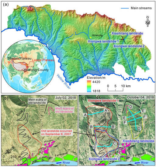
Figure 1.
(a) Locations of the Tibetan Plateau, Loess Plateau, Hualong County, and the three adjacent landslides (Xiongwa landslides 1 and 2 and the Xiashitang landslide). (b) Pre-failure images taken on 2 July 2018. (c) Post-failure images taken on 4 October 2018. The electrical resistivity tomography (ERT) profiles AA’, BB’, and CC’ in Xiongwa landslides 1 and 2 and profiles DD’, EE’, and FF’ in the Xiashitang landslide are shown in (c).
The lithosomes of the three landslides are mainly covered by orange glutenite (interbedding hard and soft clastic rocks), which are categorized as terrigenous clastic sediments (Figure 2a). There is a weathered soil layer covered on top of the substratum with a thickness around 1–2 m, which is the weathering product of orange glutenite. Field investigation revealed that the landslide bodies mainly consist of unweathered substratum (glutenite) and weathered soil (Figure 2b,c). This orange glutenite is characterized by poor physical and mechanical properties and poor weathering resistance. Moreover, the well-developed fissures result in rocks having low strength; thus, the rocks are prone to sliding due to the formation of weak geological structures [40,41]. Thus, the hillslope is prone to sliding under the influence of rainfall.
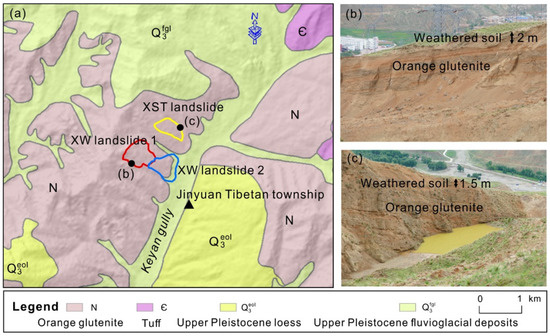
Figure 2.
Lithologic map and field investigation of the three landslides. (a) the lithologic map and location of XW landslides 1 and 2, and XST landslide. (b,c) typical profiles of the XW landslide 1 and XST landslide. A weathered soil layer covered on orange glutenite with a thickness about 1–2 m.
3. Methods
3.1. Measurement of Landslide Surface Movement Distance and Direction
The aerial images of pre-failure and post-failure moments allow us to track the movement of the surface features. Based on the aerial images obtained on 2 July 2018 (SPOT7) and 4 October 2018 (SPOT6), with a resolution of 1.5 m, the locations of the same surface features (e.g., roads) were first identified in different aerial images. Then, the same surface features were connected with lines. The lengths of the lines were measured to quantify movement distance, and the angles between the lines and north were confirmed as the movement direction of the surface features using ArcGIS 10.2 (ArcGIS by Esri). In this manner, a vector displacement field was mapped.
3.2. Time-Series InSAR and DInSAR Analyses
A total of 31 Sentinel-1 ascending orbit interferometric images acquired from 4 September 2017 to 30 August 2018, with a spatial resolution of 20.0 × 5.0 m (Azimuth × Range, A × R), were obtained from the European Space Agency (ESA). The image obtained on 10 October 2017 was chosen as the super master (Figure 3). A Shuttle Radar Topography Mission (SRTM) Digital Elevation Model (DEM) (30 m) with a vertical accuracy of ±10 m was used as the topographic reference (https://earthexplorer.usgs.gov/ (accessed on 11 June 2021)). The small-baseline subset (SBAS) technique was used to obtain cumulative displacements of the three landslides in this study. Forty-five days was taken as the temporal baseline, and 200 m was taken as the spatial baseline. The orbit datasets generated 87 interferometric pairs. We also conducted DInSAR analysis based on two pre-failure interferometric images (acquired on 18 August and 30 August 2018) and one post-failure image (acquired on 11 September 2018) in order to detect sudden movement of the landslides (Figure 4).
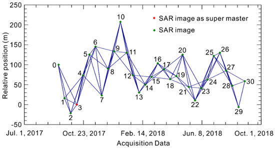
Figure 3.
Spatial and temporal baselines of the selected Sentinel-1 pairs during the period from 4 September 2017 to 30 August 2018.
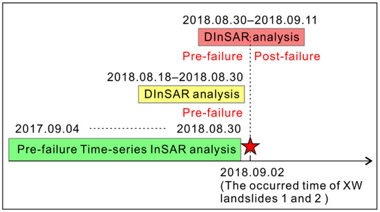
Figure 4.
Temporal coverage of the time-series InSAR analysis and DInSAR analysis.
3.3. UAV Surveys
We carried out UAV photogrammetry on 21 December 2020 and 28 June 2021 (Table 1). The UAV used was a DJI PHANTOM 4 RTK. We designated the flight heights as 300 m on the first survey and 200 m on the second survey. The flight speed was 7.9 m/s for both surveys. We set 6 and 21 ground control points (GCPs) to ensure the accuracy of the orthophotos and the DEMs in the UAV surveys, respectively. The coordinates of each GCP were measured by using a Global Navigation Satellite System Real-Time Kinematic (GNSS RTK) (CHCNAV, i50, China). The orthophoto and DEM were generated by using the Pix4Dmapper software (Pix4Dmapper, 2017). The coordinate system used was the WGS_3_Degree_GK_CM_102E. In this manner, two high-resolution DEMs and orthophotos were generated.

Table 1.
UAV flight parameters for two different surveys.
3.4. Electrical Resistivity Tomography Detection of the Internal Structures of the Landslides
Most landslides have large heterogeneities due to variations in materials and local slope topography. Electrical resistivity tomography can reveal water content distributions at different depths along a profile, which constitutes key evidence for investigating the internal structure of landslide deposits [36]. In this study, we used electrical resistivity tomography to detect the internal structures of the landslides along three profiles in XW landslides 1 and 2 and three profiles in the XST landslide. The ERT instrument used was a GeoERT IP 2401 (Beijing, China). Electrode spacing was set at 5 m, and the effective measuring depth reached about 75 m along profiles AA’, BB’, and CC’ and about 75 m, 55 m, and 55 m along profiles DD’, EE’, and FF’, respectively (Figure 1c). The coordinates of each electrode were measured by using GNSS RTK.
3.5. Effective Antecedent Precipitation
Precipitation is regarded as a key trigger for landslides in most mountainous and hilly areas. It should be noted that hillslope stability is not only influenced by the precipitation on the day of the event but also by the precipitation within a certain period preceding a landslide [42]. This is referred as to the effective antecedent precipitation, and its influence on the soil water content will gradually decay due to evaporation. Thus, we followed the method of Ma et al. [42] and Guo et al. [43] and used the effective antecedent precipitation (EAP) to evaluate the contribution of precipitation to hillslope instability:
where EAP is the effective antecedent precipitation, Pi is the daily precipitation on the ith day before the landslide, n is the number of days before the landslide (1 ≤ i ≤ n), and K is the decay coefficient due to evaporation [42]. Here, following Ma et al. [42], K was set to 0.84.
4. Results and Discussion
4.1. Evolution and Displacement of the Three Adjacent Landslides
4.1.1. Evolution of XW Landslides 1 and 2 and Its Influence
As is shown in Figure 5, road S306 was mainly destroyed by the landslides on 8 September 2007 and 2 September 2018. Historical aerial images revealed that the earlier landslide, which occurred on 8 September 2007, was located in the middle of the hillslope, and it destroyed about 2.7 km of road S306 (Figure 5b). As shown in Figure 5a, the main sliding direction of XW landslides 1 and 2 was east. Due to the fact that road S306 is the key road from Bayan Town to Guanting Town, the government had to repair the damaged road in order to ensure that traffic could pass through, but the risk of future landslides to inhabitants and their houses and farmland remained. On 2 September 2018, about 3.8 km of road S306 was destroyed again by XW landslides 1 and 2 (Figure 5d), which disrupted traffic for 10 days. Then, road S306 was repaired again after the second landslide. It is likely that this portion of road S306 will be destroyed again as the landslide region remains unstable.
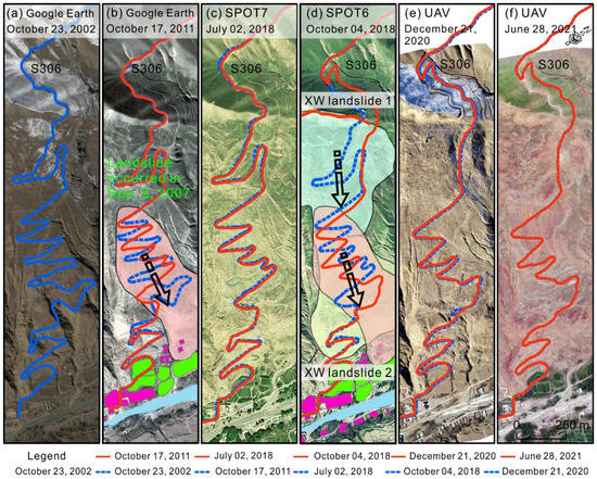
Figure 5.
Road S306 was destroyed by the landslides on 8 September 2007 and 2 September 2018. The images in (a,b) were acquired from Google Earth on 23 October 2002 and 17 October 2011, respectively. The two SPOT images in (c,d) were acquired on 2 July 2018 and 4 October 2018, respectively. The two UAV-based orthophotos in (e,f) were acquired on 21 December 2020 and 28 June 2021, respectively.
Road construction is difficult and expensive, especially in underdeveloped mountainous areas. Thus, even though the road was damaged by landslides several times, the government had to repair the road multiple times over a short period. Short-term evacuation, but not relocation, is feasible for most villages because their property, such as their houses and farmland, cannot be moved. As a result, we have to learn how to live with the risk of landslides. Fortunately, with the development of monitoring techniques, more early warning systems are being used to provide key information for hazard warning announcements.
4.1.2. Landslide Surface Movement Vector Field
Figure 6a shows that only a few points can be treated as reliable ground features and were used to identify the movement direction and distance of XW landslides 1 and 2. The main sliding direction of XW landslide 1 was east, with a mean slip distance of 93.5 m. Moreover, the local topographic features helped us to estimate the slip directions in regions 1 and 2 (black dashed circles 1 and 2 in Figure 6a). Part of the deposits moved downward into the gully, with a S–SE direction in region 1 and a N–NE direction in region 2. The ground features in the middle of the hillslope were completely destroyed, so the displacement in this region could not be identified. The results of the vector fields in XW landslide 2 indicate that the displacement in the right part (with a mean slip distance of 26.0 m) was less than that in the left part (with a mean slip distance of 81.5 m).
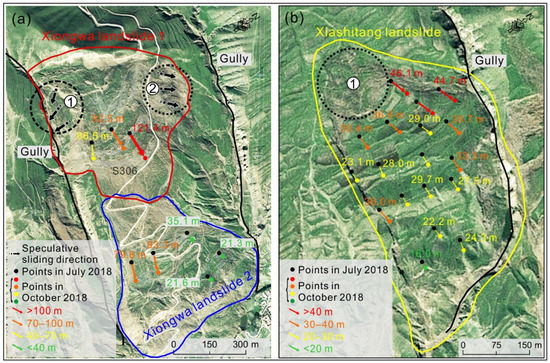
Figure 6.
Vector displacement fields of (a) Xiongwa landslides 1 and 2 and (b) the Xiashitang landslide. The vectors and numbers indicate the direction and distance, respectively, of the landslide surface features mapped via visual interpretation.
The vector displacement field shown in Figure 6b was formed based on 18 pairs of ground features, which were identified in pre-landslide and post-landslide aerial images. The vector fields of the XST landslide were completely different from those of XW landslides 1 and 2. With the exception of region 1 (black dashed circle 1 in Figure 6b), which lacked the reliable ground features needed to confirm the direction and distance of the movement, clear vector fields were obtained for the other parts of the XST landslide. Their displacements ranged from 16.0 to 46.1 m, with a mean distance of 30.9 m. Displacement gradually decreased from the NW to the SE. All of the directions of the vectors showed that the main slip direction of the XST landslide was east. The vector displacement fields demonstrated that the XST landslide was a typical retrogressive landslide; that is, the movement distance in its upper part was greater than that in its lower part. Most of the topography and geomorphology in this region differ from those of a natural hillslope due to the construction of terraced fields. These changes in topography may be the key factors that caused the old landslide and the XST landslide. The entire landslide body, except for the upper part, moved downslope, but the relative spatial positions of the surface features only changed slightly, which is key evidence confirming the movement process of the XST landslide.
4.1.3. Pre-Failure Displacement Detection Revealed by Time-Series InSAR
We used the InSAR technique to determine the pre-failure displacements of the landslides from 4 September 2017 to 30 August 2018. Figure 7 shows the cumulative displacements of the three landslides. We found that only the area along road S306 exhibited a small displacement and that most of the regions did not exhibit significant displacement for XW landslide 1. In particular, the main scarp region of XW landslide 1 was almost stable. Thus, the XW landslide was a sudden landslide, and its short deformation period was less than the Sentinel-1 satellite revisit period (minimum of 6 days). The cumulative displacement of XW landslide 2, except for point L6, was less than 11 mm, illustrating that XW landslide 2 was also still stable, except for the toe region (point P6) (Figure 7b). However, the cumulative deformation of the XST landslide gradually increased from 4 September 2017 to 30 August 2018. Figure 7c–e illustrates that the instability occurred in the upper part of the XST landslide first and then the deformation area gradually increased (Figure 7f–i). From 20 June 2018 to 30 August 2018, except for the upper part of the XST landslide, the main landslide body exhibited clear displacement (Figure 7j,k). The time-series InSAR analysis revealed that the displacement at the top of the XST landslide was negligible since this part did not move downward, but it was cracked by the movement of the main body. This is also key evidence for illustrating that the XST landslide was a retrogressive landslide.
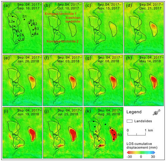
Figure 7.
Cumulative displacement in Xiongwa landslides 1 and 2 and the Xiashitang landslide areas from 4 September 2017 to 30 August 2018. The cumulative displacements of points L1–L6, R1–R4, and S1 were identified and are shown in (a). (b–k) Time-series displacement cumulation in different period.
Figure 8c shows that the displacement at point R2 in the XST landslide was larger than those at points R3 and R4, which were larger than that at point R1. Moreover, the upper part of the XST landslide failed first (Point R2 in Figure 8a). This is consistent with the results of the surface movement vector field based on pre-failure and post-failure aerial images. As cumulative displacement increased, the lower part of the landslide moved downward due to the extrusion of material in the upper part. Thus, the XST landslide was a typical retrogressive landslide.
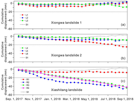
Figure 8.
The cumulative displacement of typical points in (a) Xiongwa landslide 1, (b) Xiongwa landslide 2, and (c) the Xiashitang landslide. The locations of the points are shown in Figure 7a.
4.1.4. Large Displacement Detection Revealed via DInSAR
An obvious phase jump was identified based on the interferograms of two adjacent periods. It corresponds to severe low coherence, which means that a large amount of displacement occurred in a short period of time. It general, this can be treated as the signal of the landslide’s occurrence and can be used to identify where the larger deformation occurred [19]. Figure 9a,b show that most of the parts of XW landslides 1 and 2 did not exhibit significant interferometric fringes and were characterized by a higher correlation. Thus, XW landslides 1 and 2 remained stable until 30 August 2018. However, the significant interferometric fringes (Figure 9c) and low correlation (Figure 9d) indicate that a larger displacement occurred in XW landslides 1 and 2 and part of the XST landslide from 30 August to 11 September 2018. This DInSAR analysis provides key evidence of the occurrences of larger displacements, which means that XW landslides 1 and 2 occurred without significant early deformation until 30 August 2018.
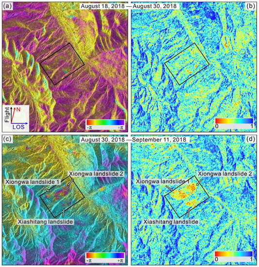
Figure 9.
SAR Interferograms and coherence of Xiongwa landslides 1 and 2 and the Xiashitang landslide based on the ascending image pairs for (a,b) 18–30 August 2018 and (c,d) 30 August–11 September 2018.
Most landslides around the world are preceded by deformations [15,24]. Deformation detection of landslides that remain stable until several days or even one day before their failure is undoubtedly difficult when using time-series InSAR analysis because Sentinel-1 images have a relatively long repeating period (minimum of 6 days). For example, for Shuicheng landslide—which occurred on 23 July 2019, killed 42 people, and destroyed 21 houses in Guizhou, China—even in the latest image, which was acquired on 20 July 2019 (three days before the landslide), the surface deformation process was not detected via multitemporal InSAR [22]. Thus, the InSAR technique can track the movement processes of some potential landslides, but it ignores some unstable slopes that may transform into catastrophic landslides. We have to learn how to live with this risk because natural hazards are unavoidable and numerous landslides still cannot be detected [44]. The early warning of landslides is still a challenge even with the development of the Earth observation system, InSAR, UAV surveys, and in situ monitoring sensors. Determining where and when landslides will occur still requires further study [15].
4.2. Surface and Subsurface Characteristics of the Three Adjacent Landslides
4.2.1. Surface Characteristics Based on UAV and Field Investigations
We conducted field investigations and UAV surveys on 21 December 2020 and 28 June 2021. Figure 10a–d shows that XW landslides 1 and 2 tore apart the hillslope surface. Most of the damage to the road and hillslope surface was X-shaped. A witness reported that XW landslide 1 began as collapses in the main scarp area (Figure 10a) on the morning of 2 September 2018, and the entire hillslope moved slowly downward until the afternoon [45]. The deformation and movement processes of XW landslides 1 and 2 were different from those of the landslides characterized by long-runout distances and great mobility. The unstable material of latter landslides is usually semi-fluid, and it quickly slides along the surface. However, the main body of XW landslides 1 and 2 did not exhibit obvious liquefaction and, thus, moved slowly, which caused most of the parts of the landslide body to deform several times due to interactions between the material and local topography. The entire unstable hillslope length (including XW landslides 1 and 2) was more than 1200 m. Figure 10b,c shows that the damaged road exhibited a different shape, which indicates that the stress conditions varied in different parts of XW landslides 1 and 2.
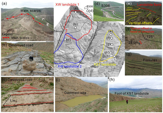
Figure 10.
Field investigation of Xiongwa landslides 1 and 2, as well as the Xiashitang landslide. (a) the main scarps of XW landslide 1. (b,c) the destroyed road due to the XW landslides 1 and 2. (d) the destroyed road S306. (e,f) vertical offsets in head of the XST landslide. (g) typical fissures in the XST landslide. (h) the foot of the XST landslide. (i) the dammed lake in the toe of the XST landslide.
The XST landslide was a reactivated landslide, which was located in an old landslide body (Figure 1c). Figure 10e shows that the head of the XST landslide was cracked and formed several vertical offsets. In contrast, the foot of the XST landslide was not significantly deformed since part of the deposition was transported into the river along the gully. Two dammed lakes formed in the toe the XST landslide, which may become sources of debris flow (Figure 10i). Thus, the houses and farmland located in the toe are still threatened.
High resolution UAV-based DEMs and orthophotos have become powerful methods in landslide surveying and mapping [46,47]. Here, by using a UAV-based DEM obtained on 28 June 2021, which was resampled to a 2.5 m resolution in ArcGIS 10.2, in addition to an Advanced Land Observing Satellite World 3-D Digital Surface Model (AW3D DSM) [48] obtained from 2006 to 2011 with a resolution of 2.5 m, we examined elevation differences during pre-failure and post-failure periods by using the Raster Calculator tool in ArcGIS 10.2. Figure 11a,e show that the upper and middle parts of the hillslope were actually destroyed by two landslides, i.e., XW landslides 1 and 2, respectively. Moreover, the slope (Figure 11c) and hillshade (Figure 11d) clearly show the main scarp of XW landslide 2, which was difficult to identify in the orthophotos (Figure 11b). Although part of the landslide body has been artificial disturbed, the pre-failure and post-failure characteristics of profile A–D still show the erosion and deposition regions of each landslide.
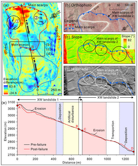
Figure 11.
UAV surveys showing that the failure of XW landslide 1 triggered the XW landslide 2. (a) Elevation differences revealed by AW3D DSM (pre-failure) UAV-based DEM (post-failure). (b) Orthophoto, (c) slope, and (d) hillshade on main scarp of XW landslide 2. (e) Elevation changes along profile A–D during pre-failure and post-failure stages.
4.2.2. Electrical Resistivity Tomography Detection of the Internal Structures of Landslides
We used electrical resistivity tomography to investigate the influence of landslides with different movement processes on internal structures along six profiles (Figure 1c). Figure 10 shows the distribution of the electrical resistivity in the XST landslide along profile DD’ after four iteration calculations. The significant electrical resistivity changes are interpreted as a possible shear surface. The depth of the shear surface varies from 20 to 40 m along the profile. Most of the region above the shear surface is characterized by lower electrical resistivities (<10 Ωm). The region below the shear surface has a higher electrical resistivity than compared to the surrounding area (>60 Ωm) and could be bedrock or compacted soil. In the upper part of the XST landslide (upper 200 m) (red irregular region 1 in Figure 12a), surface cracks promote water infiltration and result in this region having high-water content.
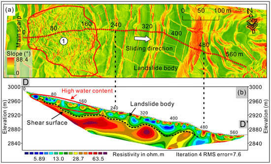
Figure 12.
(a) Slope along profile DD’ in the Xiashitang landslide and (b) internal structure detection of the Xiashitang landslide based on ERT.
Figure 13 shows the distributions of electrical resistivity in the XST landslide along profiles EE’ and FF’ after four and five iteration calculations, respectively. Profile EE’ is nearly perpendicular to the sliding direction and is longer than the landslide’s boundary (Figure 13a). We found that both landslide flank regions (black and blue dashed circles in Figure 13b) are characterized by lower electrical resistivity values than the surrounding areas, which indicates that where soil structure has been disturbed, the water concentration is higher. According to the differences in the electrical resistivity, we speculate that the shear surface along profile EE’ varied from 20 to 25 m in depth. The landslide body has lower electrical resistivities than the bedrock region. The same pattern was found along profile FF’ (Figure 13d), but the shear surface along profile FF’ varied from 15 to 45 m in depth. This indicates that the depth of the XST landslide varied in different parts of the landslide, which may have been caused by local topography and soil properties.
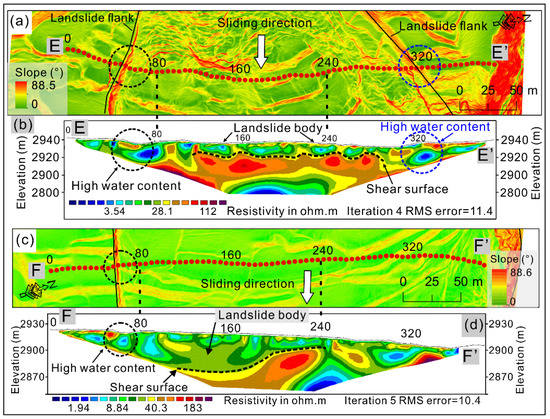
Figure 13.
(a,c) Slope along profiles EE’ and FF’ in the Xiashitang landslide. (b,d) Internal structure detection of the Xiashitang landslide based on ERT.
Figure 14 shows the distribution of electrical resistivities in XW landslides 1 and 2, which are the result of five iteration calculations, along profiles AA’, BB’, and CC’ to a maximum depth of about 70 m. Shear surface recognition of XW landslides 1 and 2 from electrical resistivity tomography was difficult because the landslides are characterized by significant heterogeneities along the profiles and with depth, which makes them difficult to identify in 2D images. The post-failure road repair also changed the surface structure (to a depth of about 5 m) and affected the electrical resistivity of the soil. However, the locations of the road and damaged road are characterized by a larger resistivity (Figure 14).
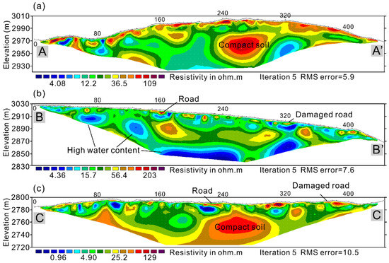
Figure 14.
Internal structure detection of the Xiongwa landslide based on electrical resistivity tomography (ERT) along profiles (a) AA, (b) BB′, and (c) CC’.
Electrical resistivity tomography has been widely used to detect the internal structures of landslides based on 2D or 3D images of the spatial distribution of electrical resistivities [36]. ERT provides us with an opportunity to understand the landslide’s internal structure without using boreholes. However, the internal structure was not speculated based on the exact value of the electrical resistivity but on its spatial distribution characteristics and even on the stratigraphic data from boreholes [34,36]. In our study, the electrical resistivity tomography profiles illustrate that XW landslides 1 and 2 were characterized by cracked surfaces and significant internal heterogeneities. This is the complex result of the influence of multiple deformations between deposition periods and local topography, as well as human activities. Compared with the XW landslides, the XST landslide may have a clear shear surface since it is a retrogressive landslide. Both the time-series InSAR analysis and surface movement vector fields illustrate that the main body flowed down as a whole. Thus, the ERT technique may be more suitable for detecting the internal structure of landslides similar to XST.
4.3. Possible Triggering Factors of the Landslides
4.3.1. Effective Antecedent Precipitation
Precipitation intensity is a common and easily accessible landslide warning signal. It is crucial for hazard warnings in most mountainous and hilly areas, especially in the under-developed regions where there is a lack of ground-based sensors obtaining deformation information of unstable hillslopes [46,47,48,49,50,51,52]. However, daily precipitation on 2 September 2018 (timing of XW landslides 1 and 2) was only 0.4 mm. We suggest that cumulative effective antecedent precipitation (EAP) may have played a key role in the occurrences of these landslides. According to the China Meteorological Administration [53], the number of heavy rainfall days (25 mm < precipitation < 50 mm within 24 h) was seven during the study period (Figure 15). The EAP on 2 September 2018 reached 34.8 mm (n = 7) and 39.0 mm (n = 10). Thus, although the daily precipitation on 2 September 2018 was only 0.4 mm, the landslides occurred due to the effect of the antecedent precipitation. Moreover, this study area is mainly covered by layered clastic rocks (Figure 2). The poor physical and mechanical properties of clastic rocks render them more susceptible to sliding than compared to other hard rocks, such as intrusive rocks [40,41]. The strength of clastic rocks is also significantly influenced by water content. Thus, effective antecedent precipitation played a key role in landslide failure.
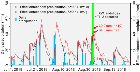
Figure 15.
Daily precipitation and effective antecedent precipitation from 1 July 2018 to 30 September 2018 at the Tuwacang meteorological station. K is the decay coefficient due to evaporation, and n is the days before the landslide. Here, K was identified as 0.84.
In fact, EAP is a key parameter in most landslide early warning systems, which are based on precipitation thresholds, e.g., the daily rainfall in 24 h and the cumulative rainfall in the previous 15 days are used for landslide advisory in Hong Kong [54]. In the Seattle area, USA, the empirical rainfall thresholds for landslides were confirmed to be a result of antecedent precipitation 3–15 days before landslide activity [49,55]. Landslides triggered by EAP are always potentially catastrophic because villagers have lowered their alertness. Thus, longer rainfall durations, even when each daily amount of rainfall is small, always results in a larger EAP for landslide occurrences. More attention should be paid to EAP, especially in under-developed mountainous regions.
4.3.2. Influence of Adjacent Landslides
Rainfall, earthquakes, and anthropogenic activities such as road construction, irrigation, and coal mining are responsible for the occurrences of most landslides [56,57,58,59,60,61,62]. In this study, we found that the deformation of an existing landslide itself can also trigger new adjacent landslides. In fact, many studies have reported that early landslides are likely to cause subsequent landslides in adjacent areas due to local topography and morphology changes caused by earlier landslides [63,64]. The degree of overlap between earlier and later landslides is a key assessment factor for previous landslides triggering later landslides [3,64]. In this study, we calculated the degree of overlap between the old landslide, which occurred on 8 September 2007, and the XW landslides 1 and 2, which occurred on 2 September 2018, following Samia et al. [64]. The result showed that 56.8% of XW landslide 2 spatially overlapped the older landslide (Figure 1 b,c and Figure 5b). Thus, the XW landslide 2 may be reactivated with a larger scale due to the extrusion of the XW landslide 1. Hillslope remained in a critical state after the previous landslide. This means that the topographic instabilities remaining after an earlier landslide need to be removed by further mass movement. In this manner, the failure of XW landslide 1 became a key trigger for the reactivation of the old landslide on a larger scale.
5. Conclusions
In this study, we observed three landslides that occurred on adjacent hillslopes in the same period and were characterized by different movement processes using UAV surveys, time-series InSAR and DInSAR analyses, and electrical resistivity tomography. This combination of methods provided us with the opportunity to obtain a better understanding of the landslide processes in the surface and subsurface regions of these landslides. Road S306 was torn apart by XW landslides 1 and 2 on 2 September 2018. The UAV and field investigations revealed that the hillslope was deformed due to interaction between landslide materials and local topography. Only a few of the surface features could be used to build a surface movement vector field. Based on time-series InSAR and DInSAR analyses, we confirmed that the XW landslides 1 and 2 occurred suddenly without significant early deformations under the effect of effective antecedent precipitation. Moreover, the poor physical and mechanical properties of clastic rocks were also key factors in the formation of multiple landslides. We found that the failure of XW landslide 1 was partly in response to XW landslide 2. This means that a landslide can also trigger another landslide under special topographic and local natural conditions. However, the XST landslide, which occurred on an adjacent hillslope, is a typical retrogressive landslide that occurred through slow creep deformation over about one year and eventually slipped. Our results suggest that InSAR detection of regional potential hazards may have difficulty identifying some catastrophic landslides that lack significant early deformation. We need to learn to live with the risk of landslides because natural hazards are unavoidable.
Author Contributions
Conceptualization, H.Q. and M.C.; methodology, D.Y. and H.Q.; software, Y.Z., Z.L. and Y.L.; investigation, Y.P., S.M., C.D. and H.S.; writing—original draft preparation, D.Y.; writing—review and editing, H.Q. All authors have read and agreed to the published version of the manuscript.
Funding
This work was funded by the Second Tibetan Plateau Scientific Expedition and Research Program (STEP) (Grant No. 2019QZKK0902), Natural Science Basic Research Program of Shaanxi (Grant No. 2021JC-40), and International Science and Technology Cooperation Program of China (Grant No. 2018YFE0100100).
Institutional Review Board Statement
Not applicable.
Informed Consent Statement
Not applicable.
Data Availability Statement
The data presented in this study are available upon request from the corresponding author.
Acknowledgments
We thank the China Meteorological Data Service Center for providing meteorological data.
Conflicts of Interest
The authors declare that there are no conflicts of interest.
References
- Qiu, H.; Cui, P.; Regmi, A.D.; Hu, S.; Wang, X.; Zhang, Y.; He, Y. Influence of topography and volume on mobility of loess slides within different slip surfaces. Catena 2017, 157, 180–188. [Google Scholar] [CrossRef]
- Cogan, J.; Gratchev, I.; Wang, G. Rainfall-induced shallow landslides caused by ex-Tropical Cyclone Debbie, 31 March 2017. Landslides 2018, 15, 1215–1221. [Google Scholar] [CrossRef]
- Yano, A.; Shinohara, Y.; Tsunetaka, H.; Mizuno, H.; Kubota, T. Distribution of landslides caused by heavy rainfall events and an earthquake in northern Aso Volcano, Japan from 1955 to 2016. Geomorphology 2019, 327, 533–541. [Google Scholar] [CrossRef]
- Ma, S.; Xu, C.; Xu, X.; He, X.; Qian, H.; Jiao, Q.; Gao, W.; Yang, H.; Cui, Y.; Zhang, P.; et al. Characteristics and causes of the landslide on July 23, 2019 in Shuicheng, Guizhou Province, China. Landslides 2020, 17, 1441–1452. [Google Scholar] [CrossRef]
- Turner, D.; Lucieer, A.; De Jong, S.M. Time Series Analysis of Landslide Dynamics Using an Unmanned Aerial Vehicle (UAV). Remote Sens. 2015, 7, 1736–1757. [Google Scholar] [CrossRef] [Green Version]
- Booth, A.M.; McCarley, J.C.; Nelson, J. Multi-year, three-dimensional landslide surface deformation from repeat lidar and response to precipitation: Mill Gulch earthflow, California. Landslides 2020, 17, 1283–1296. [Google Scholar] [CrossRef]
- Li, K.; Wang, Y.-F.; Lin, Q.-W.; Cheng, Q.-G.; Wu, Y. Experiments on granular flow behavior and deposit characteristics: Implications for rock avalanche kinematics. Landslides 2021, 18, 1779–1799. [Google Scholar] [CrossRef]
- Pánek, T.; Břežný, M.; Kilnar, J.; Winocur, D. Complex causes of landslides after ice sheet retreat: Post-LGM mass movements in the Northern Patagonian Icefield region. Sci. Total Environ. 2021, 758, 143684. [Google Scholar] [CrossRef] [PubMed]
- Liu, D.; Cui, Y.; Wang, H.; Jin, W.; Wu, C.; Bazai, N.A.; Zhang, G.; Carling, P.A.; Chen, H. Assessment of local outburst flood risk from successive landslides: Case study of Baige landslide-dammed lake, upper Jinsha river, eastern Tibet. J. Hydrol. 2021, 599, 126294. [Google Scholar] [CrossRef]
- Cui, Y.; Zhou, X.J.; Guo, C.X. Experimental study on the moving characteristics of fine grains in wide grading unconsolidated soil under heavy rainfall. J. Mt. Sci. 2017, 14, 417–431. [Google Scholar] [CrossRef]
- Okura, Y.; Kitahara, H.; Kawanami, A.; Kurokawa, U. Topography and volume effects on travel distance of surface failure. Eng. Geol. 2003, 67, 243–254. [Google Scholar] [CrossRef]
- Handwerger, A.L.; Roering, J.J.; Schmidt, D.A. Controls on the seasonal deformation of slow-moving landslides. Earth Planet. Sci. Lett. 2013, 377–378, 239–247. [Google Scholar] [CrossRef]
- Massey, C.; Petley, D.; McSaveney, M. Patterns of movement in reactivated landslides. Eng. Geol. 2013, 159, 1–19. [Google Scholar] [CrossRef]
- Peng, D.; Xu, Q.; Liu, F.; He, Y.; Zhang, S.; Qi, X.; Zhao, K.; Zhang, X. Distribution and failure modes of the landslides in Heitai terrace, China. Eng. Geol. 2018, 236, 97–110. [Google Scholar] [CrossRef]
- Dai, K.; Li, Z.; Xu, Q.; Bürgmann, R.; Milledge, D.G.; Tomas, R.; Liu, J. Entering the era of earth observation-based landslide warning systems: A novel and exciting framework. IEEE Geosci. Remote Sens. Mag. 2020, 8, 136–153. [Google Scholar] [CrossRef] [Green Version]
- Marschalko, M.; Yilmaz, I.; Bednárik, M.; Kubečka, K. Influence of underground mining activities on the slope deformation genesis: Doubrava Vrchovec, Doubrava Ujala and Staric case studies from Czech Republic. Eng. Geol. 2012, 147, 37–51. [Google Scholar] [CrossRef]
- Tao, T.; Liu, J.; Qu, X.; Gao, F. Real-time monitoring rapid ground subsidence using GNSS and Vondrak filter. Acta Geophys. 2018, 67, 133–140. [Google Scholar] [CrossRef]
- European Space Agency. Geophysical Measurements. Available online: https://sentinel.esa.int/web/sentinel/user-guides/sentinel-1-sar/product-overview/geophysical-measurements (accessed on 15 June 2020).
- Xu, Y.; Schulz, W.H.; Lu, Z.; Kim, J.; Baxtrom, K. Geologic controls of slow-moving landslides near the US West Coast. Landslides 2021, 18, 3353–3365. [Google Scholar] [CrossRef]
- Xu, Q.; Peng, D.; Zhang, S.; Zhu, X.; He, C.; Qi, X.; Zhao, K.; Xiu, D.; Ju, N. Successful implementations of a real-time and intelligent early warning system for loess landslides on the Heifangtai terrace, China. Eng. Geol. 2020, 278, 105817. [Google Scholar] [CrossRef]
- Massonnet, D.; Rossi, M.; Carmona, C.; Adragna, F.; Peltzer, G.; Feigl, K.; Rabaute, T. The displacement field of the Landers earthquake mapped by radar interferometry. Nature 1993, 364, 138–142. [Google Scholar] [CrossRef]
- Zhao, W.; Wang, R.; Liu, X.; Ju, N.; Xie, M. Field survey of a catastrophic high-speed long-runout landslide in Jichang Town, Shuicheng County, Guizhou, China, on July 23, 2019. Landslides 2020, 17, 1415–1427. [Google Scholar] [CrossRef]
- Wasowski, J.; Bovenga, F. Investigating landslides and unstable slopes with satellite Multi Temporal Interferometry: Current issues and future perspectives. Eng. Geol. 2014, 174, 103–138. [Google Scholar] [CrossRef]
- Squarzoni, G.; Bayer, B.; Franceschini, S.; Simoni, A. Pre-and post-failure dynamics of landslides in the Northern Apennines revealed by space-borne synthetic aperture radar interferometry (InSAR). Geomorphology 2020, 369, 107353. [Google Scholar] [CrossRef]
- Bardi, F.; Frodella, W.; Ciampalini, A.; Bianchini, S.; Del Ventisette, C.; Gigli, G.; Fanti, R.; Moretti, S.; Basile, G.; Casagli, N. Integration between ground based and satellite SAR data in landslide mapping: The San Fratello case study. Geomorphology 2014, 223, 45–60. [Google Scholar] [CrossRef]
- Intrieri, E.; Raspini, F.; Fumagalli, A.; Lu, P.; Del Conte, S.; Farina, P.; Allievi, J.; Ferretti, A.; Casagli, N. The Maoxian landslide as seen from space: Detecting precursors of failure with Sentinel-1 data. Landslides 2018, 15, 123–133. [Google Scholar] [CrossRef] [Green Version]
- Zhang, Y.; Meng, X.; Dijkstra, T.; Jordan, C.; Chen, G.; Zeng, R.; Novellino, A. Forecasting the magnitude of potential landslides based on InSAR techniques. Remote Sens. Environ. 2020, 241, 111738. [Google Scholar] [CrossRef]
- Ciuffi, P.; Bayer, B.; Berti, M.; Franceschini, S.; Simoni, A. Deformation Detection in Cyclic Landslides Prior to Their Reactivation Using Two-Pass Satellite Interferometry. Appl. Sci. 2021, 11, 3156. [Google Scholar] [CrossRef]
- Peyret, M.; Djamour, Y.; Rizza, M.; Ritz, J.-F.; Hurtrez, J.-E.; Goudarzi, M.; Nankali, H.; Chéry, J.; Le Dortz, K.; Uri, F. Monitoring of the large slow Kahrod landslide in Alborz mountain range (Iran) by GPS and SAR interferometry. Eng. Geol. 2008, 100, 131–141. [Google Scholar] [CrossRef]
- Li, M.; Zhang, L.; Dong, J.; Tang, M.; Shi, X.; Liao, M.; Xu, Q. Characterization of pre- and post-failure displacements of the Huangnibazi landslide in Li County with multi-source satellite observations. Eng. Geol. 2019, 257, 105140. [Google Scholar] [CrossRef]
- Bovenga, F.; Pasquariello, G.; Pellicani, R.; Refice, A.; Spilotro, G. Landslide monitoring for risk mitigation by using corner reflector and satellite SAR interferometry: The large landslide of Carlantino (Italy). Catena 2017, 151, 49–62. [Google Scholar] [CrossRef]
- Lacroix, P.; Bièvre, G.; Pathier, E.; Kniess, U.; Jongmans, D. Use of Sentinel-2 images for the detection of precursory motions before landslide failures. Remote Sens. Environ. 2018, 215, 507–516. [Google Scholar] [CrossRef]
- Zhu, Q.; Zeng, H.; Ding, Y.; Xie, X.; Liu, F.; Zhang, L.; He, H. A review of major potential landslides hazards analysis. Act Geod. Cartogr. Sin. 2019, 48, 1551–1561. (In Chinese) [Google Scholar]
- Popescu, M.; Serban, R.; Urdea, P.; Onaca, A.L. Conventional geophysical surveys for landslide investigations: Two case studies from Romania. Carpath. J. Earth Environ. Sci. 2016, 11, 281–292. [Google Scholar]
- Loke, M.H.; Chambers, J.E.; Rucker, D.F.; Kuras, O.; Wilkinson, P.B. Recent developments in the direct-current geoelectrical imaging method. J. Appl. Geophys. 2013, 95, 135–156. [Google Scholar] [CrossRef]
- Perrone, A.; Lapenna, V.; Piscitelli, S. Electrical resistivity tomography technique for landslide investigation: A review. Earth-Sci. Rev. 2014, 135, 65–82. [Google Scholar] [CrossRef]
- Hallal, N.; Chaouche, A.Y.; Hamai, L.; Lamali, A.; Dubois, L.; Mohammedi, Y.; Hamidatou, M.; Djadia, L.; Abtout, A. Spatiotemporal evolution of the El Biar landslide (Algiers): New field observation data constrained by ground-penetrating radar investigations. Bull. Int. Assoc. Eng. Geol. 2019, 78, 5653–5670. [Google Scholar] [CrossRef]
- Yao, T.; Thompson, L.; Yang, W.; Yu, W.; Gao, Y.; Guo, X.; Joswiak, D. Different glacier status with atmospheric circulations in Tibetan Plateau and surroundings. Nat. Clim. Chang. 2012, 2, 663–667. [Google Scholar] [CrossRef]
- Qin, D.; Yao, T.; Chen, F.; Zhang, T.; Meng, X. Uplift of the Tibetan Plateau and its environmental impacts. Quat. Res. 2014, 81, 397–399. [Google Scholar] [CrossRef]
- Maharaj, R.J. Landslide processes and landslide susceptibility analysis from an upland watershed: A case study from St. Andrew, Jamaica, West Indies. Eng. Geol. 1993, 34, 53–79. [Google Scholar] [CrossRef]
- Duman, T.Y. The largest landslide dam in Turkey: Tortum landslide. Eng. Geol. 2009, 104, 66–79. [Google Scholar] [CrossRef]
- Ma, T.; Li, C.; Lu, Z.; Wang, B. An effective antecedent precipitation model derived from the power-law relationship between landslide occurrence and rainfall level. Geomorphology 2014, 216, 187–192. [Google Scholar] [CrossRef]
- Guo, C.; Zhang, Y.; Montgomery, D.R.; Du, Y.; Zhang, G.; Wang, S. How unusual is the long-runout of the earthquake-triggered giant Luanshibao landslide, Tibetan Plateau, China? Geomorphology 2016, 259, 145–154. [Google Scholar] [CrossRef]
- Del Ventisette, C.; Righini, G.; Moretti, S.; Casagli, N. Multitemporal landslides inventory map updating using space-borne SAR analysis. Int. J. Appl. Earth Obs. Geoinf. 2014, 30, 238–246. [Google Scholar] [CrossRef] [Green Version]
- CCTV.com. Available online: http://news.cctv.com/2018/09/09/VIDEkVACWuCK8ON7CBiIX6uA180909.shtml (accessed on 20 July 2021).
- Al-Rawabdeh, A.; He, F.; Moussa, A.; El-Sheimy, N.; Habib, A. Using an Unmanned Aerial Vehicle-Based Digital Imaging System to Derive a 3D Point Cloud for Landslide Scarp Recognition. Remote Sens. 2016, 8, 95. [Google Scholar] [CrossRef] [Green Version]
- Yang, D.; Qiu, H.; Hu, S.; Pei, Y.; Wang, X.; Du, C.; Long, Y.; Cao, M. Influence of successive landslides on topographic changes revealed by multitemporal high-resolution UAS-based DEM. Catena 2021, 202, 105229. [Google Scholar] [CrossRef]
- Takaku, J.; Tadono, T.; Tsutsui, K.; Ichikawa, M. Validation of’aw3d’global dsm generated from alos prism. ISPRS Ann. Photogramm. Remote Sens. Spat. Inf. Sci. 2016, 3, 25. [Google Scholar] [CrossRef] [Green Version]
- Chleborad, A.F. In Preliminary Evaluation of a Precipitation Threshold for Anticipating the Occurrence of Landslides in the Seattle, Washington, Aarea; US Geological Survey Open-File Report 03-463. 2003. Available online: http://pubs.usgs.gov/of/2003/ofr-03-463/ (accessed on 13 November 2021).
- Devoli, G.; Tiranti, D.; Cremonini, R.; Sund, M.; Boje, S. Comparison of landslide forecasting services in Piedmont (Italy) and Norway, illustrated by events in late spring 2013. Nat. Hazards Earth Syst. Sci. 2018, 18, 1351–1372. [Google Scholar] [CrossRef] [Green Version]
- Liu, Y.; Qiu, H.; Yang, D.; Liu, Z.; Ma, S.; Pei, Y.; Zhang, J.; Tang, B. Deformation responses of landslides to seasonal rainfall based on InSAR and wavelet analysis. Landslides 2021, 1–12. [Google Scholar] [CrossRef]
- Liu, Z.; Qiu, H.; Ma, S.; Yang, D.; Pei, Y.; Du, C.; Sun, H.; Hu, S.; Zhu, Y. Surface displacement and topographic change analysis of the Changhe landslide on 14 September 2019, China. Landslides 2021, 18, 1471–1483. [Google Scholar] [CrossRef]
- CMA. China Meteorological Administration 2019. Available online: http://www.cma.gov.cn (accessed on 12 May 2021). (In Chinese)
- Lumb, P. Slope failures in Hong Kong. Q. J. Eng. Geol. Hydrogeol. 1975, 8, 31–65. [Google Scholar] [CrossRef]
- Godt, J.W.; Baum, R.L.; Chleborad, A.F. Rainfall characteristics for shallow landsliding in Seattle, Washington, USA. Earth Surf. Process. Landf. 2006, 31, 97–110. [Google Scholar] [CrossRef]
- Kamp, U.; Growley, B.J.; Khattak, G.A.; Owen, L.A. GIS-based landslide susceptibility mapping for the 2005 Kashmir earthquake region. Geomorphology 2008, 101, 631–642. [Google Scholar] [CrossRef]
- Xu, L.; Qiao, X.; Wu, C.; Iqbal, J.; Dai, F. Causes of landslide recurrence in a loess platform with respect to hydrological processes. Nat. Hazards 2012, 64, 1657–1670. [Google Scholar] [CrossRef]
- Zhang, F.; Huang, X. Trend and spatiotemporal distribution of fatal landslides triggered by non-seismic effects in China. Landslides 2018, 15, 1663–1674. [Google Scholar] [CrossRef]
- Qiu, H.; Cui, Y.; Pei, Y.; Yang, D.; Hu, S.; Wang, X.; Ma, S. Temporal patterns of nonseismically triggered landslides in Shaanxi Province, China. Catena 2020, 187, 104356. [Google Scholar] [CrossRef]
- Wang, J.; Jin, W.; Cui, Y.-F.; Zhang, W.-F.; Wu, C.-H.; Alessandro, P. Earthquake-triggered landslides affecting a UNESCO Natural Site: The 2017 Jiuzhaigou Earthquake in the World National Park, China. J. Mt. Sci. 2018, 15, 1412–1428. [Google Scholar] [CrossRef]
- Cui, Y.; Cheng, D.; Choi, C.E.; Jin, W.; Lei, Y.; Kargel, J.S. The cost of rapid and haphazard urbanization: Lessons learned from the Freetown landslide disaster. Landslides 2019, 16, 1167–1176. [Google Scholar] [CrossRef] [Green Version]
- Yang, D.; Qiu, H.; Ma, S.; Liu, Z.; Du, C.; Zhu, Y.; Cao, M. Slow surface subsidence and its impact on shallow loess landslides in a coal mining area. CATENA 2022, 209, 105830. [Google Scholar] [CrossRef]
- Yang, D.; Qiu, H.; Hu, S.; Zhu, Y.; Cui, Y.; Du, C.; Liu, Z.; Pei, Y.; Cao, M. Spatiotemporal distribution and evolution characteristics of successive landslides on the Heifangtai tableland of the Chinese Loess Plateau. Geomorphology 2021, 378, 107619. [Google Scholar] [CrossRef]
- Samia, J.; Temme, A.; Bregt, A.; Wallinga, J.; Guzzetti, F.; Ardizzone, F.; Rossi, M. Characterization and quantification of path dependency in landslide susceptibility. Geomorphology 2017, 292, 16–24. [Google Scholar] [CrossRef]
Publisher’s Note: MDPI stays neutral with regard to jurisdictional claims in published maps and institutional affiliations. |
© 2021 by the authors. Licensee MDPI, Basel, Switzerland. This article is an open access article distributed under the terms and conditions of the Creative Commons Attribution (CC BY) license (https://creativecommons.org/licenses/by/4.0/).