Article

Disturbance Mapping in Arctic Tundra Improved by a Planning Workflow for Drone Studies: Advancing Tools for Future Ecosystem Monitoring

1
Department of Arctic and Marine Biology, UiT The Arctic University of Norway, 9037 Tromsø, Norway
2
Fram Centre, Norwegian Polar Institute, 9296 Tromsø, Norway
3
Department of Ecoscience, Aarhus University, 8410 Rønde, Denmark
4
Department of Biology—Ecoinformatics and Biodiversity, Aarhus University, 8000 Aarhus C, Denmark
5
CIRGEO Interdepartmental Research Center of Geomatics, TESAF Department, University of Padova, Viale dell’Università 16, 35020 Legnaro, Italy
*
Author to whom correspondence should be addressed.
Remote Sens. 2021, 13(21), 4466; https://doi.org/10.3390/rs13214466
Submission received: 23 September 2021 / Revised: 27 October 2021 / Accepted: 2 November 2021 / Published: 6 November 2021

Abstract

:
The Arctic is under great pressure due to climate change. Drones are increasingly used as a tool in ecology and may be especially valuable in rapidly changing and remote landscapes, as can be found in the Arctic. For effective applications of drones, decisions of both ecological and technical character are needed. Here, we provide our method planning workflow for generating ground-cover maps with drones for ecological monitoring purposes. The workflow includes the selection of variables, layer resolutions, ground-cover classes and the development and validation of models. We implemented this workflow in a case study of the Arctic tundra to develop vegetation maps, including disturbed vegetation, at three study sites in Svalbard. For each site, we generated a high-resolution map of tundra vegetation using supervised random forest (RF) classifiers based on four spectral bands, the normalized difference vegetation index (NDVI) and three types of terrain variables—all derived from drone imagery. Our classifiers distinguished up to 15 different ground-cover classes, including two classes that identify vegetation state changes due to disturbance caused by herbivory (i.e., goose grubbing) and winter damage (i.e., ‘rain-on-snow’ and thaw-freeze). Areas classified as goose grubbing or winter damage had lower NDVI values than their undisturbed counterparts. The predictive ability of site-specific RF models was good (macro-F1 scores between 83% and 85%), but the area of the grubbing class was overestimated in parts of the moss tundra. A direct transfer of the models between study sites was not possible (macro-F1 scores under 50%). We show that drone image analysis can be an asset for studying future vegetation state changes on local scales in Arctic tundra ecosystems and encourage ecologists to use our tailored workflow to integrate drone mapping into long-term monitoring programs.

Graphical Abstract

1. Introduction

Rapid climate change is altering abiotic and biotic disturbance processes in the Arctic and could therefore lead to ecosystem state changes in tundra ecosystems [1,2,3,4]. Abiotic disturbances to the Arctic tundra may increase due to summer warming, leading to, e.g., permafrost collapse and erosion, whereas changes in the winter climate cause, for instance, rain-on-snow events and ground ice, permafrost thaw and changes of hydrological regimes [2,5,6,7,8,9,10,11]. In addition, climate change can also modify the intensity and frequency of biotic disturbances to tundra, e.g., via herbivore grazing [12,13]. The cumulative effect of changes in multiple drivers can thus alter the state of tundra ecosystems [14]. Ecosystem state changes can be detected by mapping vegetation or tundra surface types, quantifying, for example, increases in forest or shrub cover [15,16], or assessing variables such as vegetation type composition and percentage of bare ground-cover [17,18]. While these examples illustrate that some ecosystem state changes have happened in the Arctic, it remains to be documented by means of long-term monitoring, which ecosystem states continue to develop in an Arctic landscape that is facing rapid environmental change [14].
High Arctic tundra, such as in Svalbard, represents an ecosystem in high demand for monitoring [3,13], as new biotic and abiotic conditions are evolving fast with rapid climate change. In particular, the winter climate in Svalbard has, since the late 1990s, seen a regime shift towards more frequent rain-on-snow events due to mild temperatures and, consequently, more pronounced formation of basal ice [19] that encapsulates and damages plants [20]. This commonly occurs in low-land tundra with, e.g., dwarf shrub vegetation [21]. Additionally, increasing herbivore populations (e.g., goose and reindeer) can cause biotic disturbances [12,22]. In Svalbard, a mode of herbivory with particular importance to the tundra is pink-footed goose (Anser brachyrhynchus) grubbing, which disrupts the vegetation by removing plants and the moss layer [23,24,25]. The population of pink-footed geese has increased dramatically since the 1990s [26], and heavy grubbing can remove enough vegetation to cause patches of bare ground, potentially leading to soil erosion, destabilizing permafrost and changes in the soil-carbon cycle [14,27,28,29]. Warmer summers can destabilize the permafrost further but simultaneously also lead to higher primary production and above-ground biomass [30]. Effects of summer warming, changed winter climate and altered herbivory are expected to change the current state of this high Arctic ecosystem [14]. The disturbances described above commonly cover only small areas but occur frequently across the landscape, resulting in a heterogeneous tundra where the vegetation is interspersed with different types of disturbed patches. Detecting such disturbances at the landscape scale requires new, improved monitoring methods [14].
Drones have become more accessible in recent years and allow researchers to cover larger spatial extents at multiple temporal scales [31]. Drone images provide spatial grain sizes that allow studying ecological processes at local scales in highly heterogeneous landscapes. They can help transferring from local and detailed knowledge to broad-scale environments with more spatial and temporal complexity and can improve the interpretation of satellite imagery [32]. In the Arctic, drones have been used for vegetation mapping [33,34,35], measurements of cryosphere characteristics [36,37,38,39,40,41,42,43,44,45], observations of permafrost thaw [46,47] and to help bridge the gap between field- and satellite-derived data [32,35,48]. Long-term monitoring is stated as a goal in many recently published drone studies (e.g., [49,50]), but as the technology is quite new, few current studies have compared results from drone data between years or even within the same season [32,35].
Ecological monitoring is based on comparable, repeated measurements and requires robust methodology at all steps from data collection to statistical inference. Monitoring that is based on comparisons of drone images across time (seasons, years) or space (between different areas) faces methodological challenges for obtaining consistent and comparable data [51,52,53]. Recent studies have developed guidelines for drone data acquisition, geometric processing and radiometric calibrations [31,53,54]. This helps ecologists obtain high-quality images that would allow for temporal and spatial comparison. There has been less attention on how to systematically analyze these images to extract ecological variables relevant for monitoring an ecosystem state’s changes resulting from environmental drivers. Arctic ecological monitoring programs (e.g., [55,56,57,58]), networks [59] and drone ecologists, in general, are tasked with finding the balance between their scientific interests and technical remote sensing abilities. The use of drones as a tool in ecology will therefore benefit from shared protocols that go beyond the first steps of image acquisition and processing. To better capture ecosystem changes, we need to include further steps in the overall workflow, such as variable selection, layer resolution, ground-cover class selection and model development, including ground calibration and validation [31,53].
The overall aim of our study is to test ways of using drone imagery to collect variables that will be important to describe vegetation state changes resulting from abiotic and biotic disturbance factors that currently frequently occur at our study sites in Svalbard. For this purpose, we develop a method planning workflow with a focus on the steps after image acquisition (Table 1) to serve as guidance for the use of drone images in tundra ecological monitoring.

2. Material and Methods
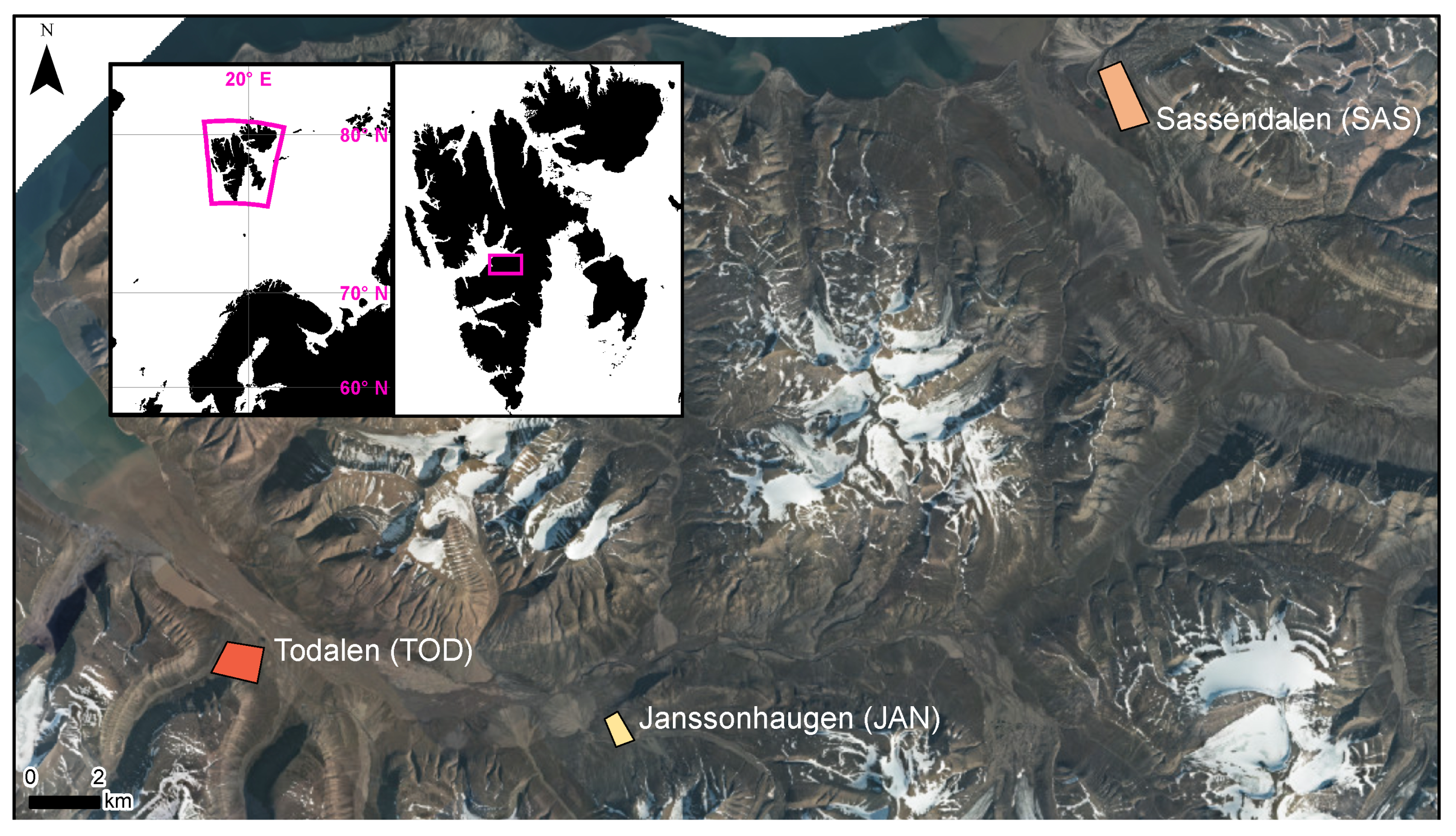
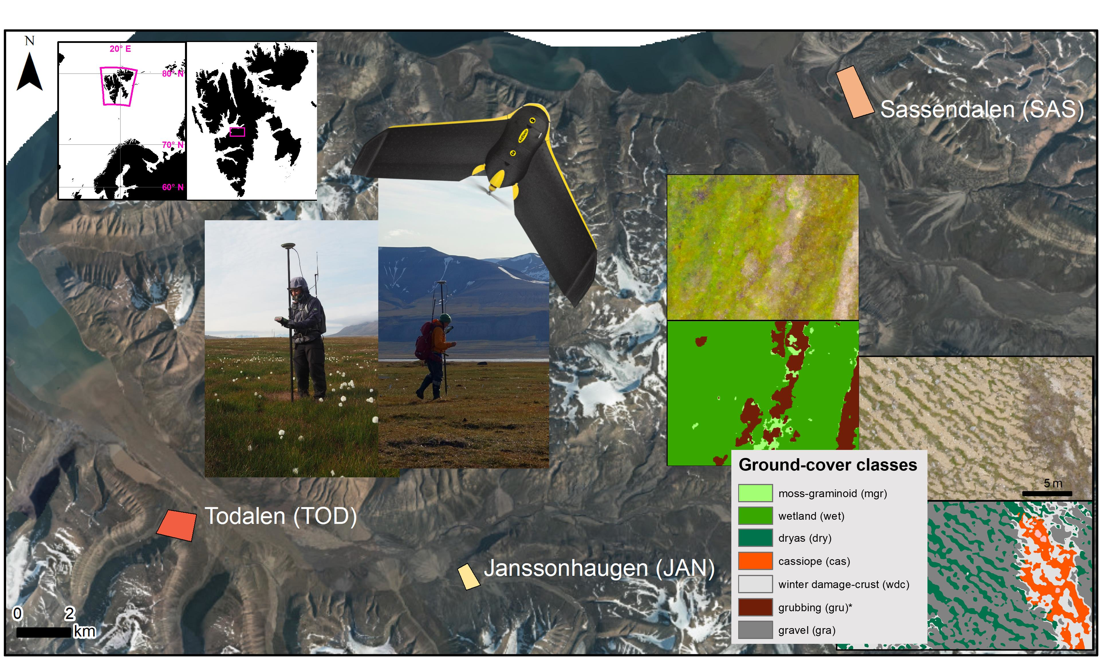
2.1. Study System

Svalbard is a high Arctic archipelago (74 ° –81 ° N, 10 ° –35 ° E), where only 15% of the land is vegetated [71,72]. Our three study sites (Janssonhaugen (JAN), Sassendalen (SAS) and Todalen (TOD)) are located in Nordenskiöld Land in the center of the main island, Spitsbergen (Figure 1). The area is characterized by glacial valleys with continuous vegetation at low elevations and sparse to no vegetation at higher elevations and on mountain slopes [73]. The study sites have similar plant community compositions, and each spans a gradient from moist-mesic tundra mires to dry-mesic ridges [74]. More information on the plant communities can be found in Appendix A. Annual precipitation is around 190 mm [75], and soils range from hyperskeletic cryosols in the moist moss tundra, haplic cryosols in the dry ridges and turbic cryosols where thaw-freeze cycles perturbate the ground (based on descriptions of Migala et al. [76]).

2.2. Study Preparation

We developed a workflow (see Table 1) to systematically plan the data collection and analysis steps of our study.

2.3. Data Collection

Our data collection choices are based on considerations presented in Table 1—(1) Flight planning. We captured aerial images during plant biomass peak season (20–28 July 2019) at the three study sites (Figure 1). We used a fixed wing drone (eBeeX by Sensefly) rigged with an AeriaX RGB camera and Sequoia+ four band camera (red, near infrared, red edge and green bands). As the Sequoia+ camera model is radiometrically calibrated automatically [77], we only took pictures of a spectral calibration target (Zenith Lite—SphereOptics) as backup. Image overlap was 70% or higher for the AeriaX RGB camera, while for the Sequoia+, side overlap was 60% and horizontal overlap 80%. We flew in perpendicular lines to the main slope of the terrain and kept a constant height over the ground (between 70 and 100 m above ground, depending on the camera and site) and speeds between 8–15 m/s).
Ground sampling distance (GSD) varied slightly between sites, see Figure 1. We flew around noon (earliest 10:00 latest 15:00) to have similar light conditions and avoid shadows on sunny days. We only flew on days with stable light conditions, such as blue skies (for study sites TOD, SAS) or continuous overcast (study site JAN), and wind speeds below 7 m/s. We used a Leica GS10 base station (Leica Geosystems) with an in-flight RTK (real time kinematic) link to the drone to obtain camera positions in real time and thus readily georeferenced images. We placed four ground control points (GCPs) in the area to validate spatial location accuracy, for which the maximum error was 5 cm.
We collected ground truth (GT) information, i.e., ground-cover class validation points, with the help of an accurate GPS system (Leica GS10 base station and rover) at 2 cm accuracy and real time correction. We aimed at collecting GT points spread throughout each of the study sites, with ca. 40 GT points per ground-cover class for each site, resulting in a total of 1782 GT points. We identified a total of 17 ground-cover classes, but not all classes were present at all sites. For each GT point, we noted the dominant ground-cover type in a ca. 7.5 cm radius around the point. Figure 2 illustrates the variation of the ground-cover classes. See Appendix A for detailed descriptions of each of the ground-cover classes.

2.4. Data Preparation

Using Pix4D Mapper [78], we generated five orthomosaics with images from the Sequoia+ sensor (four optical bands and the normalized difference vegetation index (NDVI)). With the same software, we created a digital surface model (DSM) using the 3D point cloud from the images of the AeriaX RGB camera. Our AeriaX RGB camera switched from manual to automatic settings during several instances and could therefore not be radiometrically calibrated. As a result, we used RGB images only to generate the DSM. We used the R (version 4.0.0.) software for all further analyses [79], and scripts can be found in the Supplementary Materials. To obtain textural information from our orthomosaics, we calculated gray level co-occurence matrices (GLCMs), as conducted in Wang et al., 2015 [61], using the R package glcm [80]. We calculated seven types of GLCMs for the NDVI, green and red edge orthomosaics and using four different neighborhood sizes (0.3 m, 0.9 m, 1.5 m, 2 m) with equal offsets in all directions as we did not expect any specific directionality in our data. Larger neighborhood sizes for the GLCMs were not computationally feasible with our setup, as processing times per variable reached multiple days. We did not include the DSM in our analysis because we found that the absolute height above sea level is not a useful predictor for generalizing across sites as it is too specific for each study site. Instead, we used it to calculate several of the terrain variables that were tested and discussed in [81]: slope at 1 m, 5 m and 10 m resolution, vector ruggedness, dissection, several curvature functions and terrain ruggedness (R package: SpatialEco [82]), all of the latter at 0.2 m and 1 m resolution using a range of neighborhoods sizes (0.6 m–2.2 m for the 0.2 m resolution, with 0.4 m intervals, and 3 m–131 m for the 1 m resolution, with 10 m intervals). We chose the smaller resolutions to capture the local heterogeneity of the terrain, such as tussocks and grubbing craters, and the larger resolutions to describe more general terrain positioning at the study sites.

2.5. Variable Selection

To reduce the number of drone-imagery-derived variables for further analyses, we used two exclusion criteria. First, we visually investigated the potential of the terrain variables to distinguish ground-cover classes by plotting maps and generating boxplots. This led us to exclude the curvature functions and terrain ruggedness and only continue with slope, vector ruggedness and dissection. Both GLCMs and terrain functions are dependent on the analysis window size (neighborhoods). For each site, we explored the GLCMs and terrain variable neighborhoods in preliminary models to assess their predictive ability for at least one of the ground-cover classes. This way we reduced the number of GLCMs from 84 to 39 and the terrain variables from 61 to 21. More detailed information on variable selection considerations can be found in Table 1—(2) Variable selection.

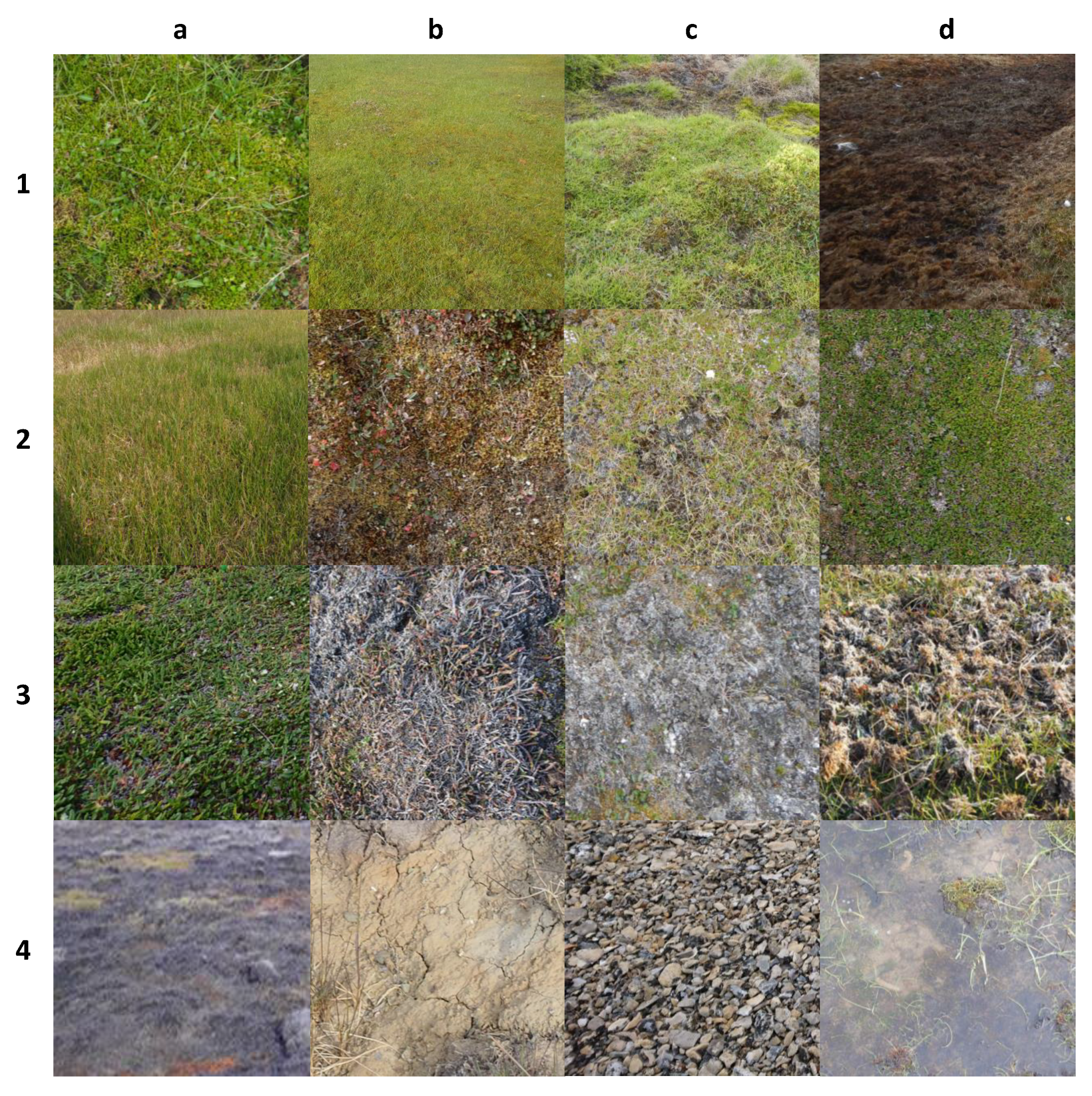
2.6. Ground-Cover Class Selection

We used a research-driven class selection approach (see Table 1—(3) Ground-cover class selection). Since the final ground-cover classes were not pre-defined, we created a flowchart to guide our decision making on how to systematically test our ability to detect ground-cover classes (Figure 3a) at different levels of detail. As a starting point of selecting ground-cover classes, we created two lists of class detail (Figure 3b). Our scheme with initial classes included all the ground-cover classes that we identified as ecologically relevant to characterize the ground. We were mostly interested in detecting disturbance ground-cover classes, and our class selection is oriented towards that. We further created a simplified classes scheme that would fulfill our minimum requirements of detecting the disturbance-related classes (bare ground, grubbing, winter damage, biological crust) and merged all vegetated classes into one. After running the classification algorithm on both schemes and evaluating the results, we created a third, optimized classes list (Figure 3b). The optimized classes differ from initial classes in three ways: (i) heath vegetation is grouped into a single class, (ii) the winter-damage-moss class is excluded as it was a very localized phenomena and challenging to validate, and (iii) the biological crust and winter damage classes are grouped into a single (mixed) class.

2.7. Data Analysis

2.7.1. Disturbance Detection Based on NDVI

In an exploratory examination, we investigated our ability of using drone images and a GSD of approximately 10 cm to detect pink-footed goose grubbing, winter damage (i.e., grey areas of dead vegetation) and bare ground (open soil). We compared the NDVI value differences of the GT points in both disturbed and undisturbed areas within the same vegetation type: For dry-mesic habitats, we compared cassiope and dryas against biological crust and winter damage. For moist-mesic habitats, we compared wetland and graminoid moss against both grubbing and bare ground. We use box-and-whisker plots to show the range of NDVI values for each study site and ground-cover class.

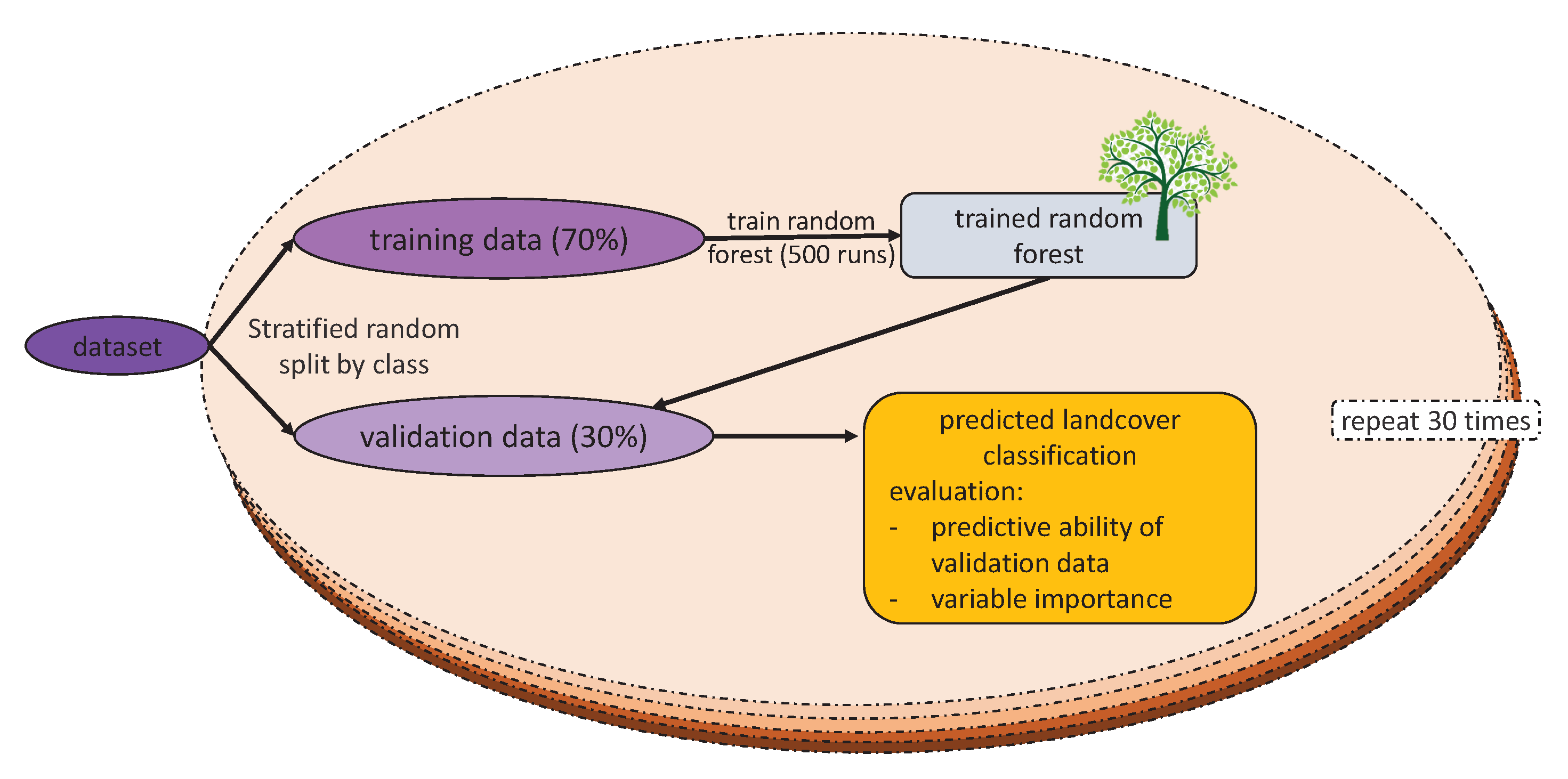
2.7.2. Classifier Development and Validation

See Table 1 for considerations on (4) Classifier development and validation. We used a random forest (RF) classifier [83] to develop ground-cover classification models for each of the study sites. We selected the RF classifier as it has been shown to be successful for spatial vegetation data [84]. For each of the study sites, we generated six RF models using three levels of detail for output classes (initial, simplified and optimized) and two sets of input variables (optical and terrain and optical only). Note that the ground-cover classification schemes differed slightly between study sites as not all classes were present at each site (Figure 3b). We used our field ground truthing (GT) data as training data by extracting the pixel values for each layer that were within the 7.5 cm radius at each GT coordinate. For some classes (snow, water, Carex subspathacea, dryas, cassiope), we lacked sufficient GT points and therefore obtained additional training data from the drone imagery. To do this, we drew polygons of the classes with insufficient training data using the RGB orthomosaics and field recordings and added all pixels within those polygons to our GT dataset.
Each RF model was developed as follows (Figure 4): we first split the extracted GT data 70–30% (stratified random, i.e., random 70–30% split within ground-cover class) into a training dataset and a validation dataset. As each GT coordinate encompassed several pixels, we reduced autocorrelation by not using any of the pixels from the same GT point for both training and validation. We then trained the RF model with the training dataset using the “fit” function (“rminer” package [85]) with ntree = 500 and a default set of mtry = 8. We tested the classifier output on the independent validation dataset using the “predict” function in “rminer”. To assess the robustness of each RF model, we repeated the process (i.e., the dataset split, model fitting and validation) thirty times. We used F1 scores to compare model performances because this measure captures both observation accuracy (recall, i.e., proportion of correctly classified pixels of a ground-cover class among all pixels belonging to that class) and prediction accuracy (precision, i.e., proportion of correctly classified pixels of a ground-cover class among all pixels classified to of that class) in a single score ( F 1 = 2 · p r e c i s i o n · r e c a l l p r e c i s i o n + r e c a l l ). F1 scores range from 0 to 100%, with values close to 100% representing high observation and high prediction accuracy. We calculated mean F1 scores for each ground-cover class and the mean macro-F1 score (arithmetic mean of all ground-cover class F1 scores) to summarize the results of the 30 cross-validation runs. We used confusion matrices to assess in more detail where class mixing occurred. In addition, we assessed the selection of predictor variables by analyzing variable importance in each of the RF models.
We created classified maps for each site with the optical and terrain option with the optimized classes. We then computed maps from these model outputs for each site using the predict function (“raster package” [86]) with parallel processing to speed up the process (ClusterR package [87]). We validated the classification by comparing the classified maps with the drone orthomosaics and hand-held pictures taken in the field.

2.7.3. Spatial Transferability

We tested how accurately a model, trained with the optimized classes developed for one study site, performed at the other two sites. First, we reduced the dataset to the ground-cover classes by excluding classes that were not present in all three sites. Then we ran the training on RF for each layer selection set (optical and terrain and optical only). Finally, we used these models to predict the ground-cover class for each pixel at the two other sites that were left out. We only tested the RF classifier transferability “as is” and did not adjust the RF trees by pruning or using transfer functions. See Table 1—(5) Transferability of classifer for more information. We used macro-F1 scores to compare the prediction outputs with one another. To gain a better understanding of the similarities between the classifiers, we compared their variable importance rankings using the mean decrease accuracy measure.

3. Results

3.1. Disturbance Detection Based on NDVI

Disturbed and associated undisturbed ground-cover types differed in their median normalized difference vegetation index (NDVI) values but had overlapping interquartile ranges. This was consistent for the three study sites (Figure 5). Most of the wetland GT points had NDVI values of 0.75 or higher, and the median of registered moss graminoid points was around 0.7. Most grubbing GT points had NDVI values that were lower than the undisturbed classes and had median values between 0.53 and 0.58. The bare ground class had the lowest NDVI, and none of the values overlapped with the undisturbed classes except for the outliers (Figure 5a). Among the drier ground-cover classes, dryas and cassiope had NDVI value medians between 0.59 and 0.75 across the three sites, whereas the classes winter damage and biological crust had median values between 0.30 and 0.48 (Figure 5b). The difference in NDVI values between the undisturbed and disturbed classes in the dry-mesic habitat was less pronounced in TOD compared to JAN and SAS.

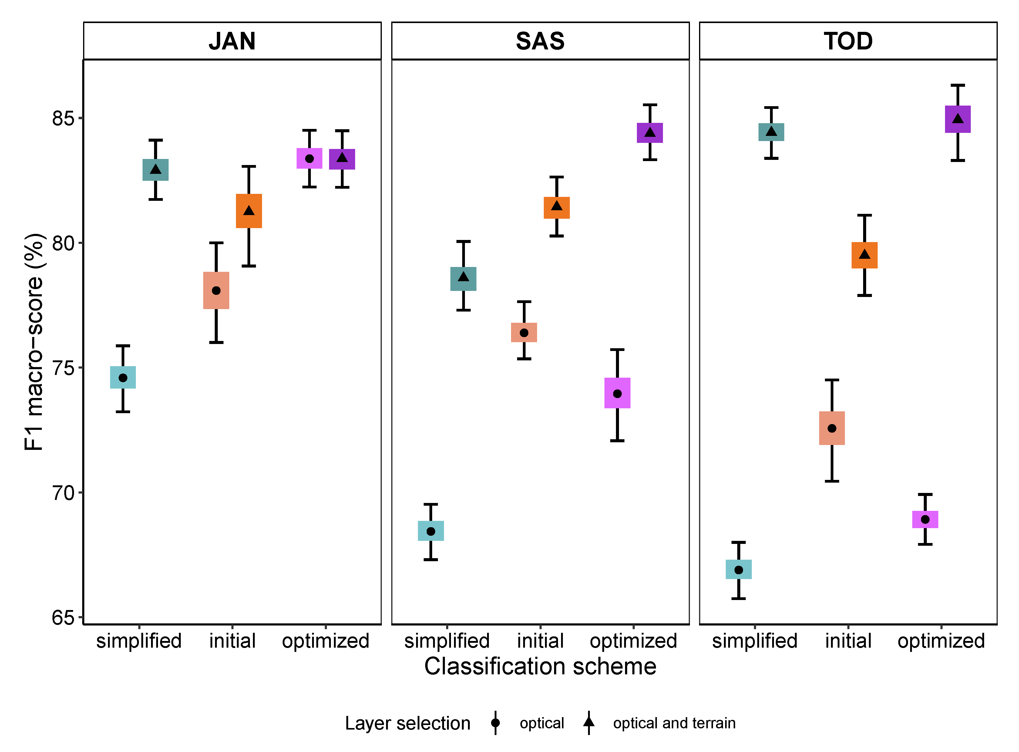
3.2. Class and Layer Selection

Comparisons of the RF classifier performances between the three classification schemes and two sets of variable selections at each site (Figure 6) showed that the ground-cover classifications based on both the terrain and optical layers had higher macro-F1 scores than the ones using only optical layers. The magnitude of the difference depended on the study site and chosen classification scheme. The classifiers using terrain and optical variables showed that: (i) the optimized classification schemes performed similarly (macro-F1 score 82–83%) in all three sites, and (ii) sites differed in terms of performance of the simplified and initial classification schemes. In site TOD, the simplified classification scheme performed better than in the sites JAN and SAS. The optimized classifier improved (compared to the initial and simplified) macro-F1 scores most in TOD.

3.3. Variable Importance

The order of importance values (measured as the mean decrease accuracy for each variable in the RF) varied between the three study sites. Among the optical variables, NDVI-based gray level co-occurence matrices (GLCM) variables were important in all three sites. NDVI was the most important layer for SAS and JAN, but ranked 19th in TOD. The terrain variables that were most important were dissection (especially at large neighborhoods) for JAN and TOD and slope for SAS. Terrain variables that were calculated at 0.2 m resolution were among the least important for predicting ground-cover classes. Complete lists with all importance values can be found in the Supplementary Materials.

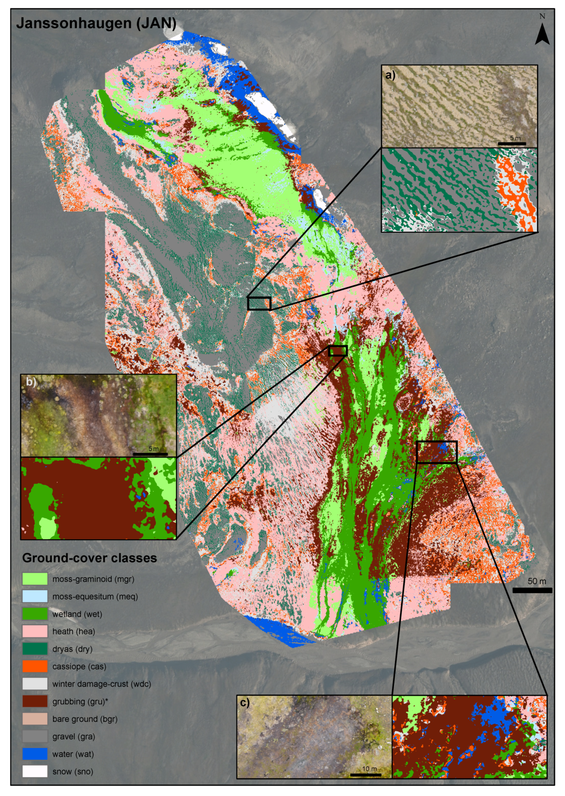
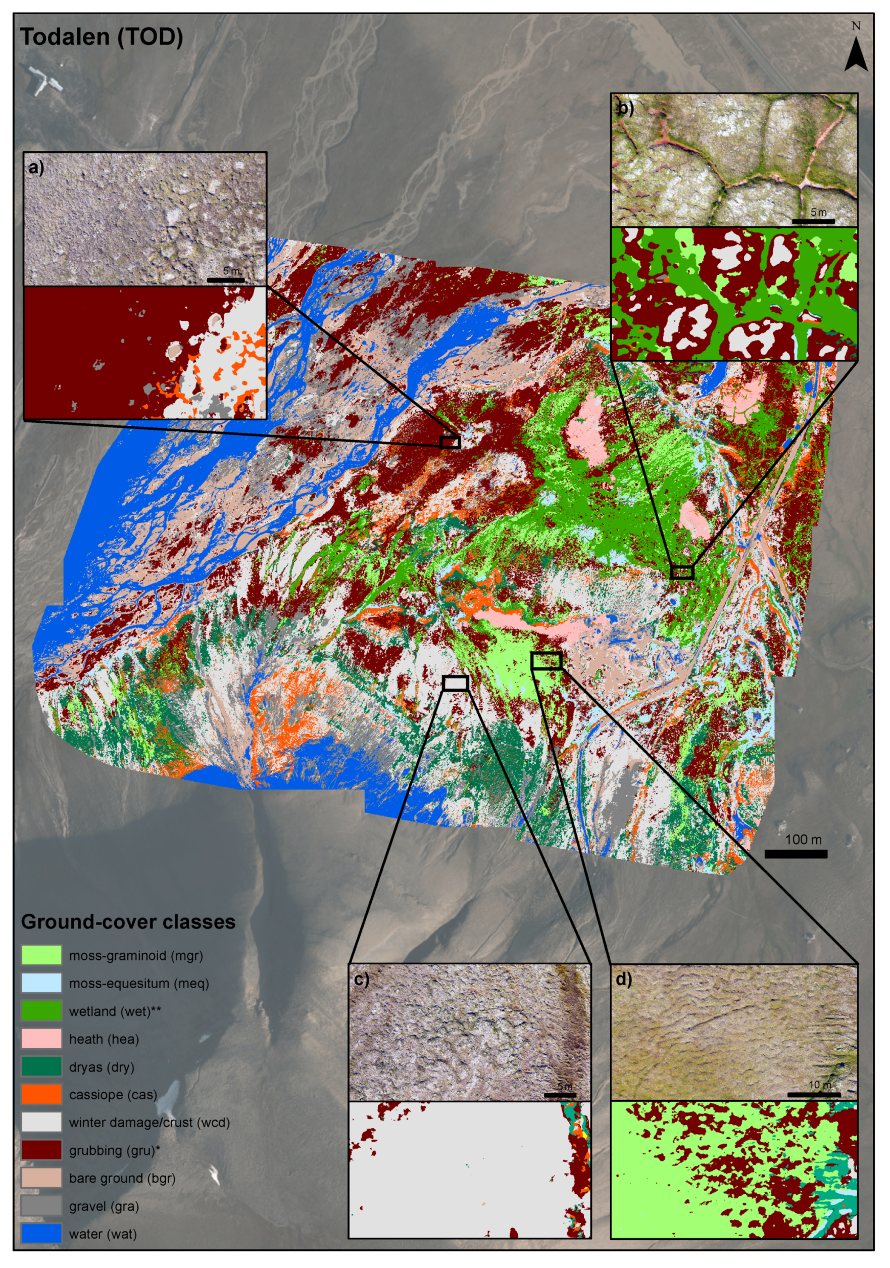
3.4. Ground-Cover Classification

Most ground-cover classes of the optimized classifier had F1 scores of 70% or higher, often over 80–90% (Table 2). The scores were generally highest for the classes snow, Carex subspathacea, water and wetland. The classes heath and gravel had the largest variation in F1 scores between study sites. There was no consistent bias in model-misclassification of the ground-cover classes in the three classifiers. Confusion matrices that show the ground-cover class distributions for each of the classifiers can be found in the Supplementary Materials. The two disturbance classes grubbing and winter damage/crust had higher observation accuracy (recall) than prediction accuracy (precision) in all three sites. Classification errors occurred mainly within the moist-mesic and the dry-mesic habitats: For example, in JAN, the most common example of misclassification was that cassiope (precision: 91.9%, recall: 72.1%) was classified as heath (precision: 67.1%, recall: 83.2%) or winter damage/crust (precision: 80.2%, recall: 87.1%). In TOD, grubbing (precision: 78.6%, recall: 78.3%) was most commonly falsely misclassfied (both directions) with the wetland (precision: 78.6%, recall: 83.0%) and graminoid-moss (precision: 88.8%, recall: 81.4%) classes.

3.5. Visual Evaluation of Predicted Ground-Cover

Based on visual inspection, the classified maps (Figure 7, Figure 8 and Figure 9) captured all ground-cover classes well. The graminoid moss tundra, the wetlands and the drier Dryas and barren classes were predicted as expected from our knowledge of the sites. Pink-footed goose grubbing was detected in graminoid moss tundra and in wetland vegetation (e.g., Figure 8b and Figure 9b,d). Winter damage/crust was detected in dry ridges, within Cassiope belts and on top of polygonal moss tundra (e.g., Figure 8c and Figure 9b). Based on our detailed in-field knowledge of the sites, there were site-specific misclassifications in “brown rugged terrain” (see discussion).

3.6. Spatial Transferability

In all cases, the models provided less accurate ground-cover classifications if trained in another site (transferred models (Figure 10). Transferability was generally highest between the sites JAN and SAS, and using only optical variables was sufficient. The highest macro-F1 score was found when using the model developed for SAS (optical variables only) to predict vegetation at JAN (macro-F1 score of 45.4%, Figure 10). Generally, transferability did not differ between using optical and terrain variables or using optical variables only. Ground-cover classes in TOD had the lowest prediction accuracy using models trained at the other study sites. Likewise, the model trained in TOD did not perform well in either of the other two study sites. The classifiers for JAN and SAS shared more of the top ten variable importance scores (see supplementary materials for details).

4. Discussion

Our case study, using drone imagery in a high Arctic tundra landscape, showed that the classification of images can be reliably used to detect both vegetation types and small-scale disturbances from herbivory and winter weather events. The workflow we developed evaluates which combination of spatial variables and ground-cover classes yields random forest (RF) models with high predictive ability. Our suggested workflow emphasizes steps in drone image processing that have previously received less attention in ecological applications. The poor transferability of models between different sites highlights that RF models are spatially specific and degrade in accuracy when applied in different spatial contexts (sites). A point worth noting is that replicability is related to the method and that each of our RF models needs to be trained with site-specific data and care must be taken when using it in another context.
The lower normalized difference vegetation index (NDVI) values for the disturbed classes winter damage/crust and grubbing compared to their non-disturbed counterparts suggest that small-scale disturbances of tundra vegetation in Svalbard can be detected correctly using drone images. However, a range of NDVI values is commonly not exclusive to a certain vegetation class (see, e.g., Raynolds et al. [88]). This was also the case for the vegetation classes and their disturbed associates in our study that had partly overlapping ranges, especially in the site TOD. A classification approach is therefore needed to distinguish among the different classes, especially in cases where repeated NDVI measurements before and after the disturbance occurred are not available.
The F1 scores for the disturbed classes were generally high (77.5–88.7%), but reaching this classifier performance required merging winter damage and biological crust to one class. More work is thus needed to distinguish the different types of biological crust that have varied coloring from white to gray and dark brown/black from winter damage in the form of dead plants that make up a gray layer on the ground. Consistently higher recall than precision values for the disturbance classes grubbing and winter damage/crust suggest high detection rates coupled with slight but consistent overestimation of these classes. Field assessments supported these findings. We detected the following inconsistencies in the predicted map compared to knowledge from the field. We recognize that grubbing was overestimated in areas with brown-colored mosses where the surface of the tundra has small-scale ruggedness due to soil movements, surface runoffs or reindeer trampling. The overestimation of grubbing also occurs in brown-colored, senescent cassiope areas and in patches of muddy water (e.g., Figure 7b,c, Figure 8a and Figure 9a, Eischeid, Ravolainen, personal observation). Winter damage/crust can be overestimated in areas with small, interspersed patches of healthy vegetation (e.g., Figure 9c, Eischeid, Ravolainen, personal observation). A mountain side shadow in the southern side of TOD was classified as water. These examples illustrate the need for additional ground-truthing and further fine-tuning of classification of the tundra vegetation types, particularly related to small-scale disturbances.
The overall high classification accuracy with macro-F1 values of over 80% for all three sites suggests that the classification performed well, comparable or better than other drone-based classifications in the high Arctic, such as Fraser et al. [89] and Thomson et al. [48]. We found no consistent bias in the misclassification of the ground-cover classes. Those misclassifications that occurred were between classes that are ecologically similar (e.g., within dry or wet habitats). The high detection of the classes moss-graminoid, moss-equisetum, wetland, Carex subspathacea and grubbing suggests that drone classification of tundra vegetation can be used to detect vegetation classes important to monitor future state changes in Svalbard’s tundra ecosystem [14]. Increases in horsetails (Equisetum spp.) and Carex subspathacea abundances were recently reported from a revisit study in central Spitsbergen [90], highlighting the importance of developing image-based methods to support field-surveys to better obtain area estimates of such changes.
Our workflow (Table 1) builds on recent publications that aimed at systematizing the collection of drone images for research in natural systems. Review articles by Aasen et al. [31], Assmann et al. [54] and Tmušic et al. [53] focused on improving reproducibility and quality of drone-based surveys, including spectral calibration, standardized data collection and general quality control. With our workflow, we expanded this set of available guidelines, focusing on variable and class selection in an ecological context of Tundra ecosystems that can help researchers make decisions on drone data processing and image analysis. With our case study, we show how the workflow helped us to make systematic choices in planning our methods, as well as testing the limitations of our data, thereby ensuring ecologically sound research that is suitable for long-term monitoring.
Variable selection can be a very time-consuming process due to the large number of variables that can be retrieved from the original high-resolution layers and requires an understanding of the studied ecosystem to pre-select suitable variables. Relevant neighborhood sizes are an aspect of this process adding to selection/weight given to terrain and optical layers. We adapted the approach of Fan and Wang et al. [61,62], who systematically pre-tested different neighborhood sizes to find the most relevant ones. Analyzing three study sites simultaneously complicated the variable selection process and increased the total number of variables used for our analysis. Common systematic approaches to reducing the number of variables often rely on reruns with lower numbers of variables to find the smallest error rates [91]. These approaches were, however, not suitable when evaluating three classifiers (three study sites) simultaneously, and we, therefore, kept all the variables after the pre-test we determined to be important in at least one of the three study sites. Similarly, we kept the feature set size (mtry = 8) constant for all sites and classifiers to reduce the possible number of model outputs and comparisons. Further work on optimizing the site-specific models would allow us to find the most important predictor variables and optimized feature set.
As part of our workflow, we compared the RF classifier outputs that were based on optical and terrain variables or optical variables only. Using both terrain and optical variables improved in-site classifications compared to using only optical variables. In other contexts, different combinations of variables can lead to the best classification. For instance, drone surveys of structural landscape changes, such as landslides or river morphology, have achieved good results using terrain information only [92,93]. The optimal set of variables will depend on plant community composition, the ground-cover classification detail needed and the types of sensors available [89,94,95,96]. We therefore recommend future drone-based ground-cover classification studies to include a wide range of variables and utilize our suggested selection procedures to find the most suitable ones for analysis.
Ground-cover classification maps have become a key resource in institutional, policy and law-making practice, but so far, there is a lack of conceptual frameworks and agreeable standards for map based monitoring [97]. Structuring ground-cover classes (i.e., in a hierarchical approach) can help with choosing appropriate class level detail and allow transferring across scales [97]. In our study, we found a structured selection approach, in line with adaptive monitoring goals [98], appropriate to find the optimal class level detail. It allowed us to focus on the ecological relevance of each of the ground-cover classes. We can therefore recommend our ground-cover class selection framework as a tool to create purpose-specific maps and find the balance between model accuracy and obtaining classes relevant for the monitoring goals.
Our results indicated low model transferability between study sites. Low regional transferability has also been reported in other RF classification studies [81,99]. Transferability can be improved by either reducing the number of classes [95], applying algorithm transfer functions, such as transformation matrices or tree pruning mechanism [69,70], or using different classifier types (e.g., [100,101]. Some deep learning approaches have recently been shown to provide classifications of drone and satellite data with reasonable transferability across space [102,103]. These approaches were outside the scope of our study as transferability was not the central goal. The right balance between a locally precise or transferable classifier will depend on the site-specific use-case, and a multi-approach framework may be needed to satisfy both local and regional monitoring requirements.

5. Conclusions

This study provides a planning workflow for generating vegetation cover maps with drones for ecological monitoring purposes in high Arctic tundra. Using random forest classifiers, we were able to successfully distinguish up to 15 different ground-cover classes, including two disturbance classes, goose grubbing and winter damage, which had lower NDVI values than their undisturbed counterparts. Although the models indicate a high predictive ability for the disturbance classes, field assessments have shown an overestimation of disturbances in parts of the moss tundra landscape. We show that a direct transfer of the models between study sites was not possible without further fine-tuning of methodologies. Future work might benefit from focusing separately on locally optimized maps and developing more generalized, transferable models. We have shown that it is possible to map the ground-cover classes that will likely be important to study state changes in Svalbard’s tundra ecosystem. Future drone times-series are necessary to work on the detection of state transitions. We encourage closer interdisciplinary collaboration between experts of remote sensing, informatics and ecology to combine the knowledge-base and further improve the quality of map-based ecological monitoring.

Supplementary Materials

The following are available online at https://www.mdpi.com/article/10.3390/rs13214466/s1.

Author Contributions

The following authors contributed with the conceptualization, I.E., R.A.I., J.M., Å.Ø.P., E.M.S. and V.T.R.; methodology: I.E., J.J.A., F.P. and V.T.R.; investigation: I.E. and V.T.R.; formal analysis: I.E., F.P. and V.T.R.; visualization: I.E. and E.M.S.; writing—original draft preparation: I.E., E.M.S., Å.Ø.P. and V.T.R., writing—review and editing: I.E., E.M.S., J.J.A., R.A.I., J.M., Å.Ø.P., F.P., N.G.Y. and V.T.R.; funding acquisition: E.M.S., R.A.I., J.M., Å.Ø.P., N.G.Y. and V.T.R. All authors have read and agreed to the published version of the manuscript.

Funding

This research was funded by the Tromsø Research Foundation and made possible by a grant from the University of Aarhus, and the Norwegian Polar Institute provided personnel and field logistics.

Data Availability Statement

The data presented in this study are available on request from the corresponding author.

Acknowledgments

We thank Stein Tore Pedersen and the Norwegian Polar Institute for providing logistic support for our field work. We thank Ingrid G. Paulsen and Torgeir T. Blæsterdalen for support in the field. We thank the Governor of Svalbard and Hurtigruten for access to field accommodation. Anne Urset and Harald Faste Aas at the NPI mapping section provided valuable support with the GPS equipment. Furthermore, we thank Rolf Andersen at the Arctic University of Norway (UiT) for providing us processing services and support for using large datasets. This publication is a contribution from the Climate-Ecological Observatory for Arctic Tundra (COAT).

Conflicts of Interest

The authors declare no conflict of interest. The funders had no role in the design of the study; in the collection, analyses, or interpretation of data; in the writing of the manuscript; or in the decision to publish the results.

Appendix A. Ground-Cover Class Descriptions

The three sites for the drone flights were chosen so that they include ground-cover classes that are of high importance in tundra plant–herbivore interactions and have effects on plants from extreme winter weather events [14]. The meso-topography of mountainous tundra landscapes causes differentiation in vegetation types within relatively short distances (e.g., Mörsdorf et al. [104]), enabling study of dry, mesic, moist and wet ground-cover classes at the the same sites.
In the high Arctic Svalbard, the drier habitats of convex landscape forms are often dominated by Dryas octopetala heath [105] that is an available and important foraging habitat to the Svalbard reindeer and rock ptarmigan in the winter [106,107]. In a lower belt, below the ridges, in central parts of Spitsbergen, there is often Cassiope tetragona vegetation that is snow-covered during the winter. Winter extreme weather with rain-on-snow events have been shown to cause damage to these dwarf shrubs [20,21], although the area extent of such damage remains to be documented. Mountain sides and slightly sloping parts of the landscapes are often covered with a thick moss layer where herbaceous plants dominate alongside Salix polaris. In the lower parts of the landscapes, the moss tundra gradually changes to wetlands with cotton grasses and grasses adapted to wet conditions. The moss tundra and wetland parts of the landscapes are important summer foraging areas for all the vertebrate herbivores [14].
These landscapes encompass a selection of functionally important habitats with high potential for change due to climate change and the dynamic herbivore populations [14,58]. The expected trajectories of change differ between the dry, moist and wet habitats and between the disturbance types [14]. This highlights the importance of developing tools to quantify changes in areas of vegetation states and areas effected by the disturbances.
Vegetation types in Svalbard have been described in various sources earlier, including a vegetation map based on satellite data [72], plant sociological and classification studies [73,108] in Svalbard’s flora [105] and in other research literature [22,30,109,110]. The previously defined vegetation state or type descriptions differ from each other depending on the purpose of the study. For our purpose of mapping especially the dwarf shrub vegetation types and the moss tundra, in combination with the most important disturbance to them (winter damage and herbivory by goose, respectively), we defined the following initial list of ground-cover classes so that it allowed us to work on vegetation and disturbances in combination.
(1a) Moss-graminoid
A common denominator for this class is a layer of mosses (typically 10–30 cm, or deeper) in moist terrain. Typical vascular plants are grasses in the genera Poa, Festuca, Alopecurus and Dupontia, the deciduous dwarf shrub Salix polaris, forbs in different genera such as Ranunculus, Saxifraga, Micranthes and Pedicularis, as well as some sedges (Carex). Moss flora is diverse, with dominant species from genera Aulacomnium, Tomentypnum and Sanionia.
(1b) Moss-equisetum
This class appears in habitats similar to the class moss-graminoid and in areas transitioning to wetland, but Equisetum arvense and Equisetum scirpoides dominate the vascular plant community.
(1c) Wetland
The wetlands in our study sites are located in slightly sloping areas and intermixed or downslope from the moist moss tundra. This class includes wetland dominated by mosses (such as Drepanocladus spp. and Scorpidium spp.) and graminoids such as Eriophorum spp. and Dupontia fisheri.
(1d) Moss-brown-wetland
This class is a specific type of wetland with less graminoids and mostly covered by wet, brown-colored mosses, giving the patches a potentially different spectral signature from 1c. This class was only mapped in TOD but also occurs in JAN and SAS, although less frequent there. These patches can be covered in water during wet years and dry out during drier years or seasons.
(2a) Carex subspathacea
This class occurs in habitats that otherwise would be classified as wetland but is characterized by a dense cover of C. subspathacea. It is one of the main arctic salt marsh plant species and has been documented to replace graminoids in areas of intensive pink-footed goose grubbing [90]. We only mapped this class in TOD, although it is also present in SAS and to a smaller extent in JAN.
(2b) Heath-moss
This class is typically found in slight depressions between ridges on the slopes and is characterized by a thin (approx. 1–5 cm) and drier moss layer often dominated by Sanionia spp. Vascular plants are usually sparse but include Salix polaris, Saxifraga oppositifolia or Cerastium spp.
(2c) Heath-graminoid
The heath-graminoid class is similar to the heath-moss class, with the difference that the moss layer is covered by graminoids, typically Luzula confusa, or in dry and convex terrain, such as Carex species.
(2d) Dryas
We assigned this class to ridges where open Dryas octopetala vegetation is found. The substrate in our dryas class is of gravel or thin silty soils on mainly alluvial deposits or terraces. Dryas octopetala occurs also in tussock tundra in Svalbard, but such Dryas areas were not common in the study sites.
(3a) Cassiope
We assigned this class if the dominant vegetation was Cassiope tetragona. This class is typically found downslope from the convex Dryas areas but above moss tundra and wetland areas where snow cover is stable in the winter.
(3b) Winter-damage-woody
This class is the disturbed counterpart to the dryas and cassiope classes. Periodic warm periods during winter result in sequential freezing that damages plant tissue, and coupled with rain, encapsulate plants with an ice coat. In addition, extreme winter warming can lead to desiccation when plants leave hibernation but cannot access water due to frozen soils [21]. Freezing temperatures after snow melt can damage plant tissues and decrease flowering success [20]. If the vegetation within a 15 cm circle was more than 80% damaged (gray), it was recorded for this class.
(3c) Biological crust
A layer of micro-organisms can cover bare soils, in which case, it is usually called biotic soil crust [111], but can also grow on damaged plants, in which case, it can be called biotic film. The biotic crust/film that is composed of a variety of bacteria, lichens and algae can grow over areas or that have been opened due to disturbances or over plants that were damaged. In our classification, we combined these two types of cryptogamic cover. The color of biotic crust can vary from almost white to gray or brown and black.
(3d) Grubbing
The grubbing class is the disturbed counterpart to the moss tundra and wetland classes. While grubbing, pink-footed geese often remove large amounts of moss in order to access the desired plant parts and opening up bare ground [27]. Grubbing can occur at different intensities. Our grubbing class describes areas where geese have removed enough moss to result in a continuous surface of dried moss interspersed with holes created by their beaks. We did not record singular holes (lighter intensity than our grubbing class). If grubbing has removed all vegetation and erosion processes have begun (higher intensity than our grubbing class), this would have been recorded as bare ground as it would not be possible to distinguish these patches from other bare areas that may have formed differently.
(4a) Winter-damage-moss
In one of our study sites, we recorded large patches of black/gray, previously moss-covered areas, probably disturbed by winter weather events. The most important process is not known but could include prolonged anaerobic conditions, freeze damage, perhaps combined with drought, but no apparent signs of fungal infections. This class was only recorded for JAN. These areas were black in color and different in appearance from the “winter-damage-woody” class.
(4b) Bare ground
This class encompasses all areas that are not covered with vegetation and have a soil substrate.
(4c) Gravel
This classes describes gravel substrates, pebbles and up over in size. It also includes rocks.
(4d) Water
The class water includes lakes, rivers, streams and surface run-offs. The water can either be clear or (in most cases) enriched with sediments and brown in color.
Snow
A small snow field was only present in JAN.

References

  1. Bhatt, U.; Walker, D.; Raynolds, M.; Comiso, J.; Epstein, H.; Jia, G.; Gens, R.; Pinzon, J.; Tucker, C.; Tweedie, C.; et al. Circumpolar Arctic Tundra Vegetation Change Is Linked to Sea Ice Decline. Earth Interact. 2010, 14, 1–20. [Google Scholar] [CrossRef] [Green Version]
  2. Meredith, M.; Sommerkorn, M.; Cassota, S.; Derksen, C.; Ekaykin, A.; Hollowed, A.; Kofinas, G.; Mackintosh, A.; Melbourne-Thomas, J.; Muelbert, M.M.C.; et al. Polar regions. In The Ocean and Cryosphere in a Changing Climate. A Special Report of the Intergovernmental Panel on Climate Change; Pörtner, H.O., Roberts, D., Masson-Delmotte, V., Zhai, P., Tignor, M., Poloczanska, E., Mintenbeck, K., Alegría, A., Nicolai, M., Okem, A., et al., Eds.; IPCC: Geneva, Switzerland, 2019; pp. 203–320. [Google Scholar]
  3. Taylor, J.; Lawler, J.; Aronsson, M.; Barry, T.; Bjorkman, A.; Christensen, T.; Coulson, S.; Cuyler, C.; Ehrich, D.; Falk, K.; et al. Arctic terrestrial biodiversity status and trends: A synopsis of science supporting the CBMP State of Arctic Terrestrial Biodiversity Report. Ambio 2020, 49, 833–847. [Google Scholar] [CrossRef] [PubMed] [Green Version]
  4. Aronsson, M.; Heiðmarsson, S.; Jóhannesdóttir, H.; Barry, T.; Braa, J.; Burns, C.; Coulson, S.; Cuyler, C.; Falk, K.; Helgason, H.; et al. State of the Arctic Terrestrial Biodiversity Report; Conservation of Arctic Flora and Fauna International Secretariat: Akureyri, Iceland, 2021. [Google Scholar]
  5. AMAP. Snow, Water, Ice and Permafrost. Summary for Policy-Makers. Arctic Monitoring and Assessment Programme (AMAP); AMAP: Oslo, Norway, 2017. [Google Scholar]
  6. Box, J.; Colgan, W.; Christensen, T.R.; Schmidt, N.; Lund, M.; Parmentier, F.J.; Brown, R.; Bhatt, U.; Euskirchen, E.; Romanovsky, V.; et al. Key indicators of Arctic climate change: 1971–2017. Environ. Res. Lett. 2019, 14, 045010. [Google Scholar] [CrossRef]
  7. Niittynen, P.; Heikkinen, R.K.; Aalto, J.; Guisan, A.; Kemppinen, J.; Luoto, M. Fine-scale tundra vegetation patterns are strongly related to winter thermal conditions. Nat. Clim. Chang. 2020, 10, 1143–1148. [Google Scholar] [CrossRef]
  8. Wrona, F.J.; Johansson, M.; Culp, J.M.; Jenkins, A.; Mård, J.; Myers-Smith, I.H.; Prowse, T.D.; Vincent, W.F.; Wookey, P.A. Transitions in Arctic ecosystems: Ecological implications of a changing hydrological regime. J. Geophys. Res. Biogeosci. 2016, 121, 650–674. [Google Scholar] [CrossRef] [Green Version]
  9. Jorgenson, M.; Shur, Y.; Pullman, E. Abrupt increase in permafrost degradation in Arctic Alaska. Geophys. Res. Lett. 2006, 33, L02503. [Google Scholar] [CrossRef]
  10. Rennert, K.J.; Roe, G.; Putkonen, J.; Bitz, C.M. Soil Thermal and Ecological Impacts of Rain on Snow Events in the Circumpolar Arctic. J. Clim. 2009, 22, 2302–2315. [Google Scholar] [CrossRef]
  11. Biskaborn, B.; Smith, S.; Noetzli, J.; Matthes, H.; Vieira, G.; Streletskiy, D.; Schoeneich, P.; Romanovsky, V.; Lewkowicz, A.; Abramov, A.; et al. Permafrost is warming at a global scale. Nat. Commun. 2019, 10, 1–11. [Google Scholar] [CrossRef] [Green Version]
  12. Kerbes, R.H.; Kotanen, P.M.; Jefferies, R.L. Destruction of Wetland Habitats by Lesser Snow Geese: A Keystone Species on the West Coast of Hudson Bay. J. Appl. Ecol. 1990, 27, 242–258. [Google Scholar] [CrossRef]
  13. Hansen, B.B.; Grøtan, V.; Aanes, R.; Sæther, B.E.; Stien, A.; Fuglei, E.; Ims, R.A.; Yoccoz, N.G.; Pedersen, Å.Ø. Climate Events Synchronize the Dynamics of a Resident Vertebrate Community in the High Arctic. Science 2013, 339, 313–315. [Google Scholar] [CrossRef] [Green Version]
  14. Ravolainen, V.; Soininen, E.M.; Jónsdóttir, I.S.; Eischeid, I.; Forchhammer, M.; van der Wal, R.; Pedersen, Å.Ø. High Arctic ecosystem states: Conceptual models of vegetation change to guide long-term monitoring and research. Ambio 2020, 49, 666–677. [Google Scholar] [CrossRef] [Green Version]
  15. Chapin, F.S., III; Woodwell, G.; Randerson, J.; Rastetter, E.; Lovett, G.; Baldocchi, D.; Clark, D.; Harmon, M.; Schimel, D.; Valentini, R.; et al. Reconciling Carbon-cycle Concepts, Terminology, and Methods. Ecosystems 2006, 9, 1041–1050. [Google Scholar] [CrossRef] [Green Version]
  16. Scheffer, M.; Carpenter, S.; Lenton, T.; Bascompte, J.; Brock, W.; Dakos, V.; van de Koppel, J.; van de Leemput, I.; Levin, S.; Nes, E.; et al. Anticipating Critical Transitions. Science 2012, 338, 344–348. [Google Scholar] [CrossRef] [Green Version]
  17. Jefferies, R.L.; Jano, A.P.; Abraham, K.F. A biotic agent promotes large-scale catastrophic change in the coastal marshes of Hudson Bay. J. Ecol. 2006, 94, 234–242. [Google Scholar] [CrossRef]
  18. Van der Wal, R. Do herbivores cause habitat degradation or vegetation state transition? Evidence from the tundra. Oikos 2006, 114, 177–186. [Google Scholar] [CrossRef]
  19. Peeters, B.; Pedersen, Å.; Loe, L.E.; Isaksen, K.; Veiberg, V.; Stien, A.; Kohler, J.; Gallet, J.C.; Aanes, R.; Hansen, B. Spatiotemporal patterns of rain-on-snow and basal ice in high Arctic Svalbard: Detection of a climate-cryosphere regime shift. Environ. Res. Lett. 2019, 14, 015002. [Google Scholar] [CrossRef]
  20. Milner, J.M.; Varpe, Ø.; van der Wal, R.; Hansen, B.B. Experimental icing affects growth, mortality, and flowering in a high Arctic dwarf shrub. Ecol. Evol. 2016, 6, 2139–2148. [Google Scholar] [CrossRef] [PubMed] [Green Version]
  21. Bjerke, J.W.; Treharne, R.; Vikhamar-Schuler, D.; Karlsen, S.R.; Ravolainen, V.; Bokhorst, S.; Phoenix, G.K.; Bochenek, Z.; Tømmervik, H. Understanding the drivers of extensive plant damage in boreal and Arctic ecosystems: Insights from field surveys in the aftermath of damage. Sci. Total Environ. 2017, 599–600, 1965–1976. [Google Scholar] [CrossRef]
  22. Speed, J.D.; Woodin, S.; Tømmervik, H.; Tamstorf, M.; Wal, R. Predicting Habitat Utilization and Extent of Ecosystem Disturbance by an Increasing Herbivore Population. Ecosystems 2009, 12, 349–359. [Google Scholar] [CrossRef]
  23. Speed, J.D.M.; Cooper, E.J.; Jónsdóttir, I.S.; Van Der Wal, R.; Woodin, S.J. Plant community properties predict vegetation resilience to herbivore disturbance in the Arctic. J. Ecol. 2010, 98, 1002–1013. [Google Scholar] [CrossRef]
  24. Pedersen, Å.Ø.; Tombre, I.; Jepsen, J.U.; Eidesen, P.B.; Fuglei, E.; Stien, A. Spatial patterns of goose grubbing suggest elevated grubbing in dry habitats linked to early snowmelt. Polar Res. 2013, 32, 19719. [Google Scholar] [CrossRef]
  25. Pedersen, A.S.; Speed, J.; Tombre, I. Prevalence of pink-footed goose grubbing in the arctic tundra increases with population expansion. Polar Biol. 2013, 36, 1569–1575. [Google Scholar] [CrossRef]
  26. Madsen, J.; Williams, J.H.; Johnson, F.A.; Tombre, I.M.; Dereliev, S.; Kuijken, E. Implementation of the first adaptive management plan for a European migratory waterbird population: The case of the Svalbard pink-footed goose Anser brachyrhynchus. Ambio 2017, 46, 275–289. [Google Scholar] [CrossRef] [PubMed] [Green Version]
  27. Fox, A.; Francis, I.; Bergersen, E. Diet and habitat use of Svalbard Pink-footed Geese Anser brachyrhynchus during arrival and pre-breeding periods in Adventdalen. Ardea 2006, 94, 691–699. [Google Scholar]
  28. Van der Wal, R.; Sjögersten, S.; Woodin, S.J.; Cooper, E.J.; Jónsdóttir, I.S.; Kuijper, D.; Fox, T.A.D.; Huiskes, A.D. Spring feeding by pink-footed geese reduces carbon stocks and sink strength in tundra ecosystems. Glob. Chang. Biol. 2007, 13, 539–545. [Google Scholar] [CrossRef]
  29. Speed, J.; Woodin, S.; Tømmervik, H.; van der Wal, R. Extrapolating herbivore-induced carbon loss across an arctic landscape. Polar Biol. 2010, 33, 789–797. [Google Scholar] [CrossRef]
  30. Van der Wal, R.; Stien, A. High-arctic plants like it hot: A long-term investigation of between-year variability in plant biomass. Ecology 2014, 95, 3414–3427. [Google Scholar] [CrossRef]
  31. Aasen, H.; Honkavaara, E.; Lucieer, A.; Zarco-Tejada, P.J. Quantitative Remote Sensing at Ultra-High Resolution with UAV Spectroscopy: A Review of Sensor Technology, Measurement Procedures, and Data Correction Workflows. Remote Sens. 2018, 10, 1091. [Google Scholar] [CrossRef] [Green Version]
  32. Assmann, J.J.; Myers-Smith, I.H.; Kerby, J.T.; Cunliffe, A.M.; Daskalova, G.N. Drone data reveal heterogeneity in tundra greenness and phenology not captured by satellites. Environ. Res. Lett. 2020, 15, 125002. [Google Scholar] [CrossRef]
  33. Lovitt, J.; Rahman, M.M.; McDermid, G.J. Assessing the Value of UAV Photogrammetry for Characterizing Terrain in Complex Peatlands. Remote Sens. 2017, 9, 715. [Google Scholar] [CrossRef] [Green Version]
  34. Lousada, M.; Pina, P.; Vieira, G.; Bandeira, L.; Mora, C. Evaluation of the use of very high resolution aerial imagery for accurate ice-wedge polygon mapping (Adventdalen, Svalbard). Sci. Total Environ. 2018, 615, 1574–1583. [Google Scholar] [CrossRef]
  35. Siewert, M.B.; Olofsson, J. Scale-dependency of Arctic ecosystem properties revealed by UAV. Environ. Res. Lett. 2020, 15, 094030. [Google Scholar] [CrossRef]
  36. Harder, P.; Schirmer, M.; Pomeroy, J.; Helgason, W. Accuracy of snow depth estimation in mountain and prairie environments by an unmanned aerial vehicle. Cryosphere 2016, 10, 2559–2571. [Google Scholar] [CrossRef] [Green Version]
  37. Pedersen, S.H.; Tamstorf, M.P.; Abermann, J.; Westergaard-Nielsen, A.; Lund, M.; Skov, K.; Sigsgaard, C.; Mylius, M.R.; Hansen, B.U.; Liston, G.E.; et al. Spatiotemporal Characteristics of Seasonal Snow Cover in Northeast Greenland from in Situ Observations. Arct. Antarct. Alp. Res. 2016, 48, 653–671. [Google Scholar] [CrossRef] [Green Version]
  38. Cimoli, E.; Marcer, M.; Vandecrux, B.; Boggild, C.E.; Williams, G.; Simonsen, S.B. Application of Low-Cost UASs and Digital Photogrammetry for High-Resolution Snow Depth Mapping in the Arctic. Remote Sens. 2017, 9, 1144. [Google Scholar] [CrossRef] [Green Version]
  39. Ewertowski, M.W.; Evans, D.J.A.; Roberts, D.H.; Tomczyk, A.M. Glacial geomorphology of the terrestrial margins of the tidewater glacier, Nordenskiöldbreen, Svalbard. J. Maps 2016, 12, 476–487. [Google Scholar] [CrossRef] [Green Version]
  40. Tonkin, T.; Midgley, N.; Cook, S.; Graham, D. Ice-cored moraine degradation mapped and quantified using an unmanned aerial vehicle: A case study from a polythermal glacier in Svalbard. Geomorphology 2016, 258, 1–10. [Google Scholar] [CrossRef] [Green Version]
  41. Phillips, E.; Everest, J.; Evans, D.J.; Finlayson, A.; Ewertowski, M.; Guild, A.; Jones, L. Concentrated, ‘pulsed’ axial glacier flow: Structural glaciological evidence from Kvíárjökull in SE Iceland. Earth Surf. Process. Landforms 2017, 42, 1901–1922. [Google Scholar] [CrossRef] [Green Version]
  42. Nehyba, S.; Hanáček, M.; Engel, Z.; Stachoň, Z. Rise and fall of a small ice-dammed lake—Role of deglaciation processes and morphology. Geomorphology 2017, 295, 662–679. [Google Scholar] [CrossRef]
  43. Jouvet, G.; Weidmann, Y.; Seguinot, J.; Funk, M.; Abe, T.; Sakakibara, D.; Seddik, H.; Sugiyama, S. Initiation of a major calving event on the Bowdoin Glacier captured by UAV photogrammetry. Cryosphere 2017, 11, 911–921. [Google Scholar] [CrossRef] [Green Version]
  44. Jones, C.; Ryan, J.; Holt, T.; Hubbard, A. Structural glaciology of Isunguata Sermia, West Greenland. J. Maps 2018, 14, 517–527. [Google Scholar] [CrossRef] [Green Version]
  45. Jouvet, G.; Weidmann, Y.; Kneib, M.; Detert, M.; Seguinot, J.; Sakakibara, D.; Sugiyama, S. Short-lived ice speed-up and plume water flow captured by a VTOL UAV give insights into subglacial hydrological system of Bowdoin Glacier. Remote Sens. Environ. 2018, 217, 389–399. [Google Scholar] [CrossRef]
  46. Van der Sluijs, J.; Kokelj, S.V.; Fraser, R.H.; Tunnicliffe, J.; Lacelle, D. Permafrost Terrain Dynamics and Infrastructure Impacts Revealed by UAV Photogrammetry and Thermal Imaging. Remote Sens. 2018, 10, 1734. [Google Scholar] [CrossRef] [Green Version]
  47. Cunliffe, A.M.; Tanski, G.; Radosavljevic, B.; Palmer, W.F.; Sachs, T.; Lantuit, H.; Kerby, J.T.; Myers-Smith, I.H. Rapid retreat of permafrost coastline observed with aerial drone photogrammetry. Cryosphere 2019, 13, 1513–1528. [Google Scholar] [CrossRef] [Green Version]
  48. Thomson, E.; Spiegel, M.; Althuizen, I.; Bass, P.; Chen, S.; Chmurzynski, A.; Halbritter, A.; Henn, J.; Jónsdóttir, I.; Klanderud, K.; et al. Multiscale mapping of plant functional groups and plant traits in the High Arctic using field spectroscopy, UAV imagery and Sentinel-2A data. Environ. Res. Lett. 2021, 16, 055006. [Google Scholar] [CrossRef]
  49. Turner, I.L.; Harley, M.D.; Drummond, C.D. UAVs for coastal surveying. Coast. Eng. 2016, 114, 19–24. [Google Scholar] [CrossRef]
  50. Gillan, J.K.; Karl, J.W.; van Leeuwen, W.J.D. Integrating drone imagery with existing rangeland monitoring programs. Environ. Monit. Assess. 2020, 192, 1–20. [Google Scholar] [CrossRef]
  51. Hoffmann, H.; Jensen, R.; Thomsen, A.; Nieto, H.; Rasmussen, J.; Friborg, T. Crop water stress maps for entire growing seasons from visible and thermal UAV imagery. Biogeosci. Discuss. 2016, 13, 6545–6563. [Google Scholar] [CrossRef] [Green Version]
  52. Tirado, S.B.; Hirsch, C.N.; Springer, N.M. UAV-based imaging platform for monitoring maize growth throughout development. Plant Direct 2020, 4, e00230. [Google Scholar] [CrossRef] [PubMed]
  53. Tmušić, G.; Manfreda, S.; Aasen, H.; James, M.R.; Gonçalves, G.; Ben-Dor, E.; Brook, A.; Polinova, M.; Arranz, J.J.; Mészáros, J.; et al. Current Practices in UAS-based Environmental Monitoring. Remote Sens. 2020, 12, 1001. [Google Scholar] [CrossRef] [Green Version]
  54. Assmann, J.J.; Kerby, J.T.; Cunliffe, A.M.; Myers-Smith, I.H. Vegetation monitoring using multispectral sensors—Best practices and lessons learned from high latitudes. J. Unmanned Veh. Syst. 2019, 7, 54–75. [Google Scholar] [CrossRef] [Green Version]
  55. Arctic Long-Term Ecological Research Site. Available online: https://arc-lter.ecosystems.mbl.edu/ (accessed on 23 October 2020).
  56. Bylot Island—Sirmilik National Park Long Term Monitoring Program. Available online: http://www.cen.ulaval.ca/bylot/en/bylothistory.php (accessed on 16 October 2020).
  57. Zackenberg Ecological Research Operations. Available online: https://g-e-m.dk/gem-localities/zackenberg-research-station/ (accessed on 23 October 2020).
  58. Ims, R.; Jepsen, J.U.; Stien, A.; Yoccoz, N.G. Science plan for COAT: Climate-ecological Observatory for Arctic Tundra; Fram Centre Report Series 1; Fram Centre: Tromsø, Norway, 2013. [Google Scholar]
  59. High-Latitude Drone Ecology Network (HiLDEN). Available online: https://arcticdrones.org/ (accessed on 4 September 2020).
  60. Zhou, Y.; Daakir, M.; Rupnik, E.; Pierrot-Deseilligny, M. A two-step approach for the correction of rolling shutter distortion in UAV photogrammetry. ISPRS J. Photogramm. Remote Sens. 2020, 160, 51–66. [Google Scholar] [CrossRef]
  61. Wang, H.; Pu, R.; Zhu, Q.; Ren, L.; Zhang, Z. Mapping health levels of Robinia pseudoacacia forests in the Yellow River delta, China, using IKONOS and Landsat 8 OLI imagery. Int. J. Remote Sens. 2015, 36, 1114–1135. [Google Scholar] [CrossRef]
  62. Fan, H. Land-cover mapping in the Nujiang Grand Canyon: Integrating spectral, textural, and topographic data in a random forest classifier. Int. J. Remote Sens. 2013, 34, 7545–7567. [Google Scholar] [CrossRef]
  63. Weinmann, M.; Jutzi, B.; Hinz, S.; Mallet, C. Semantic point cloud interpretation based on optimal neighborhoods, relevant features and efficient classifiers. ISPRS J. Photogramm. Remote Sens. 2015, 105, 286–304. [Google Scholar] [CrossRef]
  64. Mascaro, J.; Asner, G.P.; Knapp, D.E.; Kennedy-Bowdoin, T.; Martin, R.E.; Anderson, C.; Higgins, M.; Chadwick, K.D. A Tale of Two “Forests”: Random Forest Machine Learning Aids Tropical Forest Carbon Mapping. PLoS ONE 2014, 9, e85993. [Google Scholar] [CrossRef] [PubMed]
  65. Belgiu, M.; Drăguţ, L. Random forest in remote sensing: A review of applications and future directions. ISPRS J. Photogramm. Remote Sens. 2016, 114, 24–31. [Google Scholar] [CrossRef]
  66. Colditz, R.R. An Evaluation of Different Training Sample Allocation Schemes for Discrete and Continuous Land Cover Classification Using Decision Tree-Based Algorithms. Remote Sens. 2015, 7, 9655–9681. [Google Scholar] [CrossRef] [Green Version]
  67. Roberts, D.R.; Bahn, V.; Ciuti, S.; Boyce, M.S.; Elith, J.; Guillera-Arroita, G.; Hauenstein, S.; Lahoz-Monfort, J.J.; Schröder, B.; Thuiller, W.; et al. Cross-validation strategies for data with temporal, spatial, hierarchical, or phylogenetic structure. Ecography 2017, 40, 913–929. [Google Scholar] [CrossRef]
  68. Hastie, T.; Tibshirani, R.; Friedman, J. The Elements of Statistical Learning: Data Mining, Inference and Prediction, 2nd ed.; Springer: Berlin/Heidelberg, Germany, 2009. [Google Scholar]
  69. Segev, N.; Harel, M.; Mannor, S.; Crammer, K.; El-Yaniv, R. Learn on Source, Refine on Target:A Model Transfer Learning Framework with Random Forests. IEEE Trans. Pattern Anal. Mach. Intell. 2015, 39, 1811–1824. [Google Scholar] [CrossRef] [Green Version]
  70. Sukhija, S.; Krishnan, N.C. Supervised heterogeneous feature transfer via random forests. Artif. Intell. 2019, 268, 30–53. [Google Scholar] [CrossRef]
  71. Walker, D.; Raynolds, M.; Daniëls, F.; Einarsson, E.; Elvebakk, A.; Gould, W.; Katenin, A.; Kholod, S.; Markon, C.; Melnikov, E.; et al. The Circumpolar Arctic Vegetation Map. J. Veg. Sci. 2005, 16, 267–282. [Google Scholar] [CrossRef]
  72. Johansen, B.E.; Karlsen, S.R.; Tømmervik, H. Vegetation mapping of Svalbard utilising Landsat TM/ETM data. Polar Rec. 2012, 48, 47–63. [Google Scholar] [CrossRef]
  73. Elvebakk, A. A vegetation map of Svalbard on the scale 1:3.5 mill. Phytocoenologia 2005, 35, 951–967. [Google Scholar] [CrossRef]
  74. Elvebakk, A. A survey of plant associations and alliances from Svalbard. J. Veg. Sci. 1994, 5, 791–802. [Google Scholar] [CrossRef]
  75. Lawrimore, J.; Ray, R.; Applequist, S.; Korzeniewski, B.; Menne, M. Global Summary of the Month (GSOM), Version 1. In NOAA National Centers for Environmental Information. Available online: https://www.ncei.noaa.gov/access/metadata/landing-page/bin/iso?id=gov.noaa.ncdc:C00946 (accessed on 10 September 2021).
  76. Migała, K.; Wojtuń, B.; Szymański, W.; Muskała, P. Soil moisture and temperature variation under different types of tundra vegetation during the growing season: A case study from the Fuglebekken catchment, SW Spitsbergen. Catena 2014, 116, 10–18. [Google Scholar] [CrossRef]
  77. Cubero-Castan, M.; Schneider-Zapp, K.; Bellomo, M.; Shi, D.; Rehak, M.; Strecha, C. Assessment Of The Radiometric Accuracy In A Target Less Work Flow Using Pix4D Software. In Proceedings of the 2018 9th Workshop on Hyperspectral Image and Signal Processing: Evolution in Remote Sensing (WHISPERS), Amsterdam, The Netherlands, 23–26 September 2018; pp. 1–4. [Google Scholar] [CrossRef]
  78. Pix4Dmapper. Available online: https://www.pix4d.com/product/pix4dmapper-photogrammetry-software (accessed on 1 November 2021).
  79. R Core Team. R: A Language and Environment for Statistical Computing; R Foundation for Statistical Computing: Vienna, Austria, 2013. [Google Scholar]
  80. Zvoleff, A. glcm: Calculate Textures from Grey-Level Co-Occurrence Matrices (GLCMs). R Package Version 1.6.5. Available online: https://cran.r-project.org/web/packages/glcm/glcm.pdf (accessed on 1 November 2021).
  81. Maxwell, A.E.; Warner, T.A.; Strager, M.P. Predicting Palustrine Wetland Probability Using Random Forest Machine Learning and Digital Elevation Data-Derived Terrain Variables. Photogramm. Eng. Remote Sens. 2016, 82, 437–447. [Google Scholar] [CrossRef]
  82. Evans, J.S. spatialEco: Spatial Analysis and Modelling Utilities. R Package Version 1.3-2. Available online: https://cran.r-project.org/web/packages/spatialEco/spatialEco.pdf (accessed on 1 November 2021).
  83. Cutler, A.; Cutler, D.R.; Stevens, J.R. Random Forests. In Ensemble Machine Learning: Methods and Applications; Zhang, C., Ma, Y., Eds.; Springer: Boston, MA, USA, 2012; pp. 157–175. [Google Scholar] [CrossRef]
  84. Karami, M.; Westergaard-Nielsen, A.; Normand, S.; Treier, U.A.; Elberling, B.; Hansen, B.U. A phenology-based approach to the classification of Arctic tundra ecosystems in Greenland. ISPRS J. Photogramm. Remote Sens. 2018, 146, 518–529. [Google Scholar] [CrossRef]
  85. Cortez, P. rminer: Data Mining Classification and Regression Methods. R Package Version 1.4.6. Available online: https://cran.r-project.org/web/packages/spatialEco/spatialEco.pdf (accessed on 1 November 2021).
  86. Hijmans, R.J. raster: Geographic Data Analysis and Modeling. R Package Version 3.3-13. Available online: https://cran.r-project.org/web/packages/raster/raster.pdf (accessed on 1 November 2021).
  87. Mouselimis, L. ClusterR: Gaussian Mixture Models, K-Means, Mini-Batch-Kmeans, K-Medoids and Affinity Propagation Clustering. R Package Version 1.2.2. Available online: https://cran.r-project.org/web/packages/ClusterR/ClusterR.pdf (accessed on 1 November 2021).
  88. Raynolds, M.K.; Comiso, J.C.; Walker, D.A.; Verbyla, D. Relationship between satellite-derived land surface temperatures, arctic vegetation types, and NDVI. Remote Sens. Environ. 2008, 112, 1884–1894. [Google Scholar] [CrossRef]
  89. Fraser, R.H.; Olthof, I.; Lantz, T.C.; Schmitt, C. UAV photogrammetry for mapping vegetation in the low-Arctic. Arct. Sci. 2016, 2, 79–102. [Google Scholar] [CrossRef] [Green Version]
  90. Van der Wal, R.; Anderson, H.; Stien, A.; Loe, L.E.; Speed, J. Disturbance, Recovery and Tundra Vegetation Change Final Report project 17/92—to Svalbard Environmental Protection Fund. 2020. Available online: https://aura.abdn.ac.uk/bitstream/handle/2164/16573/SMF_Distrubance_recovery_veg_change.pdf;jsessionid=65802B34A907DB989FF65BD2D7FDB248?sequence=1 (accessed on 13 September 2021).
  91. Hapfelmeier, A.; Ulm, K. A new variable selection approach using Random Forests. Comput. Stat. Data Anal. 2013, 60, 50–69. [Google Scholar] [CrossRef]
  92. Rossi, G.; Tanteri, L.; Tofani, V.; Vannocci, P.; Moretti, S.; Casagli, N. Multitemporal UAV surveys for landslide mapping and characterization. Landslides 2018, 15, 1045–1052. [Google Scholar] [CrossRef] [Green Version]
  93. Özcan, O.; Özcan, O. Multi-temporal UAV based repeat monitoring of rivers sensitive to flood. J. Maps 2021, 17, 163–170. [Google Scholar] [CrossRef]
  94. Chen, J.; Yi, S.; Qin, Y.; Wang, X. Improving estimates of fractional vegetation cover based on UAV in alpine grassland on the Qinghai–Tibetan Plateau. Int. J. Remote Sens. 2016, 37, 1922–1936. [Google Scholar] [CrossRef]
  95. Miranda, V.; Pina, P.; Heleno, S.; Vieira, G.; Mora, C.; Schaefer, C.E. Monitoring recent changes of vegetation in Fildes Peninsula (King George Island, Antarctica) through satellite imagery guided by UAV surveys. Sci. Total Environ. 2020, 704, 135295. [Google Scholar] [CrossRef] [PubMed]
  96. Morgan, B.E.; Chipman, J.W.; Bolger, D.T.; Dietrich, J.T. Spatiotemporal Analysis of Vegetation Cover Change in a Large Ephemeral River: Multi-Sensor Fusion of Unmanned Aerial Vehicle (UAV) and Landsat Imagery. Remote Sens. 2021, 13, 51. [Google Scholar] [CrossRef]
  97. Cullum, C.; Rogers, K.; Brierley, G.; Witkowski, E. Ecological classification and mapping for landscape management and science: Foundations for the description of patterns and processes. Prog. Phys. Geogr. 2015, 40, 38–65. [Google Scholar] [CrossRef] [Green Version]
  98. Lindenmayer, D.B.; Likens, G.E. Adaptive monitoring: A new paradigm for long-term research and monitoring. Trends Ecol. Evol. 2009, 24, 482–486. [Google Scholar] [CrossRef] [PubMed]
  99. Juel, A.; Groom, G.B.; Svenning, J.C.; Ejrnæs, R. Spatial application of Random Forest models for fine-scale coastal vegetation classification using object based analysis of aerial orthophoto and DEM data. Int. J. Appl. Earth Obs. Geoinf. 2015, 42, 106–114. [Google Scholar] [CrossRef]
  100. Kalantar, B.; Mansor, S.B.; Sameen, M.I.; Pradhan, B.; Shafri, H.Z.M. Drone-based land-cover mapping using a fuzzy unordered rule induction algorithm integrated into object-based image analysis. Int. J. Remote Sens. 2017, 38, 2535–2556. [Google Scholar] [CrossRef]
  101. Wessel, M.; Brandmeier, M.; Tiede, D. Evaluation of Different Machine Learning Algorithms for Scalable Classification of Tree Types and Tree Species Based on Sentinel-2 Data. Remote Sens. 2018, 10, 1419. [Google Scholar] [CrossRef] [Green Version]
  102. Zhang, C.; Sargent, I.; Pan, X.; Li, H.; Gardiner, A.; Hare, J.; Atkinson, P.M. Joint Deep Learning for land cover and land use classification. Remote Sens. Environ. 2019, 221, 173–187. [Google Scholar] [CrossRef] [Green Version]
  103. Tong, X.Y.; Xia, G.S.; Lu, Q.; Shen, H.; Li, S.; You, S.; Zhang, L. Land-cover classification with high-resolution remote sensing images using transferable deep models. Remote Sens. Environ. 2020, 237, 111322. [Google Scholar] [CrossRef] [Green Version]
  104. Mörsdorf, M.A.; Ravolainen, V.T.; Yoccoz, N.G.; Thórhallsdóttir, T.E.; Jónsdóttir, I.S. Decades of Recovery From Sheep Grazing Reveal No Effects on Plant Diversity Patterns Within Icelandic Tundra Landscapes. Front. Ecol. Evol. 2021, 8, 502. [Google Scholar] [CrossRef]
  105. Rønning, O.I. Svalbards Flora; Norsk Polarinstitutt: Tromsø, Norway, 1996. [Google Scholar]
  106. Pedersen, Å.Ø.; Overrein, Ø.; Unander, S.; Fuglei, E. Svalbard Rock Ptarmigan (Lagopus Mutus Hyperboreus): A Status Report; Norwegian Polar Institute (Norsk Polarinstitutt): Tromsø, Norway, 2005. [Google Scholar]
  107. Pedersen, Å.; Paulsen, I.; Albon, S.; Arntsen, G.L.; Hansen, B.; Langvatn, R.; Loe, L.E.; Le Moullec, M.; Overrein, Ø.; Peeters, B.; et al. Svalbard Reindeer (Rangifer Tarandus Platyrhynchus): A Status Report; Rapportserie—Norsk Polarinstitutt, Norwegian Polar Institute: Tromsø, Norway, 2019. [Google Scholar]
  108. Vanderpuye, A.W.; Elvebakk, A.; Nilsen, L. Plant communities along environmental gradients of high-arctic mires in Sassendalen, Svalbard. J. Veg. Sci. 2002, 13, 875–884. [Google Scholar] [CrossRef]
  109. Eurola, S.; Hakala, A. The bird cliff vegetation of Svalbard. Aquil. Ser. Bot 1977, 15, 1–18. [Google Scholar]
  110. Jónsdóttir, I.S. Terrestrial ecosystems on Svalbard: Heterogeneity, complexity and fragility from an Arctic island perspective. In Biology and Environment: Proceedings of the Royal Irish Academy (JSTOR); Royal Irish Academy: Dublin, Ireland, 2005; pp. 155–165. [Google Scholar]
  111. Agnelli, A.; Corti, G.; Massaccesi, L.; Ventura, S.; D’Acqui, L.P. Impact of biological crusts on soil formation in polar ecosystems. Geoderma 2021, 401, 115340. [Google Scholar] [CrossRef]
Figure 1. Location of drone flights of the case study in Central Spitsbergen, JAN: 78.16996 ° N, 16.300685 ° E, 0.3 km 2 ; SAS: 78.331412 ° N, 16.974537 ° E, 1 km 2 ; TOD: 78.188762 ° N, 15.82335 ° E, 1 km 2 . Ground sampling distances (GSD) are listed for each site and camera (AeriaX RGB/Sequoia+ 4Band): JAN: 1.9 cm/9.8 cm; SAS: 2.2 cm/13.2 cm; TOD: 1.2 cm/10.3 cm. Aerial orthophoto provided by the Norwegian Polar Institute.
Remotesensing 13 04466 g001
Figure 2. Images of 16 ground-cover classes that were included in the initial classification scheme. row 1: moss-graminoid, moss-equisetum, wetland, moss-brown-wetland; row 2: Carex subspathacea, heath-moss, heath-graminoid, dryas; row 3: cassiope, winter-damage-woody, biological crust, grubbing; row 4: winter-damage-moss, bare ground, gravel, water. The class snow is not shown in this graphic. Detailed information for each class can be found in the Appendix A.
Remotesensing 13 04466 g002
Figure 3. Ground-cover class selection schemes. (a) Stages to determine ground-cover classes balancing class detail and classification accuracy. The first stage includes testing two class schemes: one with the most possible detail and one with the minimum required class detail. In the second stage, the optimal classes are determined by merging the classes that improve the classification accuracy using the simplified class scheme as a guideline for meaningful merges. (b) The initial, simplified and optimized ground-cover classes and class abbreviations used in the case study to classify tundra vegetation on Svalbard.
Remotesensing 13 04466 g003
Figure 4. Data selection process, model validation and evaluation. The classifier was developed using 70% of the dataset as training data and 30% as validation data. The dataset split and classifier was run 30 times. Classifier performance mean and variance as well as variable importance values were calculated from the outputs.
Remotesensing 13 04466 g004
Figure 5. The distribution of NDVI values of selected ground-cover classes and their associated disturbances in the three study sites: The disturbed associates of classes wetland and moss graminoid are grubbing and bare ground, and the associated disturbed classes of dryas and cassiope are winter damage and biological crust. The boxes denote the interquartile ranges of NDVI values around the median for all registered ground-truthing pixels for each ground-cover class, and dots represent outliers. The order of the images (up-down) follows the x-axis from left to right for each plot. (a) Moist-mesic habitat; (b) Dry-mesic habitat.
Remotesensing 13 04466 g005
Figure 6. Comparison of site, classification scheme and layer selection. Black symbols represent mean macro-F1 scores after 30 runs, the colored boxes indicate confidence intervals of 0.5 and the bars represent the interval at 0.95.
Remotesensing 13 04466 g006
Figure 7. Classified map of Janssonhaugen (JAN). Zoomed areas highlight examples of classifications: (a) The classification of dry-mesic habitat with dryas, cassiope, gravel and winter damage/crust. (b) Wet, brown-colored mosses classified as grubbing. (c) Winter-damaged moss, classified as grubbing and water.
Remotesensing 13 04466 g007
Figure 8. Classified map of Sassendalen (SAS). Zoomed areas highlight examples of classifications. (a) Dry and moist habitats: On the left, classification of dry-mesic habitat with gravel and a cassiope belt. On the right, moist habitat, classified as wetland and moss-graminoid, brown and rugged mosses classified as grubbing. (b) Grubbing detection in wetland area. (c) Zonation of dry-mesic ground-cover classes along a gravel ridge.
Remotesensing 13 04466 g008
Figure 9. Classified map of Todalen (TOD). Zoomed areas highlight examples of classifications. (a) Cassiope classified as grubbing. (b) Grubbing and winter damage/crust on ice wedge polygons. (c) A dry-mesic habitat with dryas, gravel and winter damage/crust classified as winter damage/crust. (d) Grubbing in moss-graminoid habitat.
Remotesensing 13 04466 g009
Figure 10. Classifier transferability between the three sites using the optimized classification scheme. Numbers inside the squares show the mean macro-F1 scores for in-site classifiers.The arrows indicate the direction and macro-F1 scores of using the classifier on the other sites. (a) Optical variables and (b) optical and terrain variables.
Remotesensing 13 04466 g010
Table 1. Method planning workflow for drone flight campaigns and image classifications in a tundra landscape. Studies for the steps where guidance has been published are referenced. Asterisks indicate the steps we included in our study.
TopicSolution
(1) Flight planning
What to consider when planning field work?Choose appropriate image overlap and camera angles for desired final product. *
Ensure that the type of the drone, the camera and flight speeds integrate well with one another to obtain high-quality images of suitable resolution and avoid blurring due to slow rolling shutter speeds [60]. *
Follow appropriate radiometric calibration guidelines. See guidelines from Aasen et al. [31], Assmann et al. [54] and Tmušic et al. [53] with advice for choices of flight line, (image) overlap, camera type, drone type, weather and sun, radiometric calibration, geolocation, ground control points and ground truthing. *
Ensure accurate geolocation of images and groundtruthing data. *
(2) Variable selection
Which variables to derive from the drone images?A priori knowledge of the landscape is important to select appropriate data layers and resolutions that represent ecologically explainable heterogeneity in the terrain. *
How to assess which of the available variables to include in a classifier?Variable importance can be ranked in a preliminary classifier using a subset of the available data [61,62]. *
Which variables best discriminate between ground-cover classes?Exploratory data analysis via visual inspection of data via plotting to detect patterns important for the classification. *
What neighborhood size to select?Neighborhood size can be ranked in a preliminary classifier using a subset of the available data [61,62]. *
Appropriate neighborhood sizes for secondary layers can be computationally derived using a minimum entropy approach [63].
Computational limits may define the minimum resolution or maximum possible neighborhood sizes [64]. *
(3) Ground-cover class selection
How to define the first choice of ground-cover classes for the classifier?Data-driven—Cluster analysis to see the separability of data without human input (unsupervised classification).
Research-driven—Considering data-driven results define classes that are present in the area of interest for monitoring or expected to change over time (supervised classifications). *
How to choose between classifier robustness and ground-cover class detail?Pre-define the ecological context of the ground-cover classes to determine which ones are meaningful to merge due to ecological similarities. *
How to increase transparency on class selection and its effects on classification accuracy?Define documentation of how the final classes, explain class merges and the research consequences of mixing classes. *
(4) Classifier development and validation
How to choose groundtruthing points?Choose areas that are representative for the ground-cover classes and large enough sample sizes [65]. *
Aim for a training data cover of approximately 0.25% of the study site [66] (recommendation based on medium-coarse grain satellite data).
Avoid spatial autocorrelation of groundtruthing points by stratified random sampling in a blocked design [67]
How to avoid overfitting the classifier?Split the dataset into training and validation datasets (such as K-fold mechanism or using random resampling) [64]. *
How to assess classifier robustness?Use an independent validation dataset for external validation [68]
If an independent dataset is not available, repeat runs of the classifier though multiple K-fold runs or repeat sampling of training and validation dataset [68]. *
Additional map validation by local experts can help discover issues that go undetected by classifier evaluation statistics. This can be conducted, for example, by visually comparing the classified map with the drone images, pictures or revisits to the site. *
(5) Transferability of classifier
How to assess the potential for transferability?Exploratory data analysis via visual inspection of data via plotting to detect trends/shifts in values across sites or time intervals. *
How to test the transferability of the classifier?Repetition of data collection in new area, creation of independent classifier and test in other area. *
How to improve the transferability of the classifier?Tree pruning, simplification of the classifier, transferability functions [69,70]
Table 2. Macro-F1 scores of ground-cover classifications at the three study sites on Svalbard using the optimized classes and all variables (optical and terrain). Explanations to the class abbreviations can be found in Figure 3b.
Class
sitemgrmeqwetmbwcsuheadrycaswdcgrubgrgrawatsno
JAN70.582.391.4--57.993.780.681.983.884.290.783.6100
SAS75.083.892.8--77.380.292.088.786.175.084.093.4-
TOD84.785.980.886.497.795.680.774.777.578.388.974.098.9-
Publisher’s Note: MDPI stays neutral with regard to jurisdictional claims in published maps and institutional affiliations.

