Article

Identifying Surface Urban Heat Island Drivers and Their Spatial Heterogeneity in China’s 281 Cities: An Empirical Study Based on Multiscale Geographically Weighted Regression

1
School of Public Administration and Policy, Renmin University of China, Beijing 100872, China
2
State Key Laboratory of Resources and Environment Information System, Institute of Geographic Sciences and Natural Resources Research, Chinese Academy of Sciences, Beijing 100101, China
3
University of Chinese Academy of Sciences, Beijing 100049, China
4
College of Management and Economics, Tianjin University, Tianjin 300072, China
5
Key Laboratory of Agricultural Remote Sensing, Ministry of Agriculture and Rural Affairs, Institute of Agricultural Resources and Regional Planning, Chinese Academy of Agricultural Sciences, Beijing 100081, China
6
Department of Chemical and Biochemical Engineering, Iowa Technology Institute, Center for Global and Regional Environmental Research, University of Iowa, Iowa City, IA 52242, USA
*
Author to whom correspondence should be addressed.
Remote Sens. 2021, 13(21), 4428; https://doi.org/10.3390/rs13214428
Submission received: 26 September 2021 / Revised: 24 October 2021 / Accepted: 1 November 2021 / Published: 3 November 2021

Abstract

:
The spatially heterogeneous nature and geographical scale of surface urban heat island (SUHI) driving mechanisms remain largely unknown, as most previous studies have focused solely on their global performance and impact strength. This paper analyzes diurnal and nocturnal SUHIs in China based on the multiscale geographically weighted regression (MGWR) model for 2005, 2010, 2015, and 2018. Compared to results obtained using the ordinary least square (OLS) model, the MGWR model has a lower corrected Akaike information criterion value and significantly improves the model’s coefficient of determination (OLS: 0.087–0.666, MGWR: 0.616–0.894). The normalized difference vegetation index (NDVI) and nighttime light (NTL) are the most critical drivers of daytime and nighttime SUHIs, respectively. In terms of model bandwidth, population and Δfine particulate matter are typically global variables, while ΔNDVI, intercept (i.e., spatial context), and NTL are local variables. The nighttime coefficient of ΔNDVI is significantly negative in the more economically developed southern coastal region, while it is significantly positive in northwestern China. Our study not only improves the understanding of the complex drivers of SUHIs from a multiscale perspective but also provides a basis for urban heat island mitigation by more precisely identifying the heterogeneity of drivers.

1. Introduction

Urbanization is a significant phenomenon of human activity that alters land use and cover [1,2,3]. One of the most widespread human-induced environmental influences of urbanization is the emergence of urban heat islands, described as higher temperature urban areas compared to rural references [4,5]. Urban heat islands (UHIs) have been widely observed worldwide in recent decades. Existing literature shows that temperature rise is closely related to energy consumption [6,7,8], air pollution [9,10], biodiversity [11,12], and the health of residents [13,14,15]. Therefore, the impacts of urban heat islands are a significant concern in urban environmental research.
Urban heat islands can be classified as canopy (CUHI) and surface (SUHI) UHIs [16,17,18]. Typically, CUHIs are quantified using observations from meteorological stations, while SUHIs are determined based on satellite remote sensing data [19]. Previous research has shown that the influence of local surface type on CUHIs obtained from stations cannot be ignored. This finding indicates that CUHIs are characterized by high spatial heterogeneity, thus reducing the reference value of point-based CUHIs to represent the thermal difference among urban and rural regions [20,21]. SUHIs are gradually attracting the attention of an increasing number of researchers due to the continued development of satellite technology.
The increasing accessibility of remote sensing data has dramatically enhanced satellite-based research of SUHI controls [22,23,24,25,26,27]. Peng et al. [28] analyzed the drivers of SUHIs on a global scale for the first time and found that vegetation was significantly correlated with reduced diurnal and nocturnal SUHIs. Zhao et al. [29] analyzed the effect of aerodynamic drag on SUHIs using 65 large cities in North America as the study area. A coarse-grained model connecting population, background climate, and UHI intensity was recently developed [30], indicating that the urban–rural differences in evapotranspiration and convection efficiency were the primary factors of warming. Priyankara et al. [31] analyzed an SUHI in the Seoul metropolitan area from the perspective of spatial processes and verified the mechanism of urban greening on the SUHI. The above studies have provided comprehensive and in-depth attribution analyses of SUHIs from multiple perspectives in different regions and at different times. However, two crucial issues have been ignored: the spatial heterogeneity and the scale of SUHI drivers.
Scale is an essential geographic concept. The general agreement by scholars in current research is that various processes can work at multiple spatial scales that are different from one another. Previous studies often distinguish between micro and macro processes and local and global processes [32,33]. For example, various processes operating at largely independent scales determine the weather and tides in a certain area [34]. SUHIs are also complex phenomena driven by multiple factors in the social economy and the ecological environment. Therefore, it is necessary to distinguish the spatial scales of the various driving factors in SUHI attribution analysis.
Previous empirical research models for SUHI driver analysis can generally be divided into two main categories. The first type includes global-scale analysis methods, such as correlation coefficients [28,35,36], ordinary least square (OLS) [37,38,39], generalized additive model (GAM) [40], and various models for machine learning [41,42,43]. The biggest problem with these methods is that they cannot adequately analyze the spatial variations of SUHI drivers, making them feasible for small regional studies but leading to obvious bias at large spatial scales, such as in China. The second category is the classical geographically weighted regression method (GWR), which has long been employed as a local regression model to address the heterogeneity problems of spatial processes [44,45,46]. However, each spatial parameter in the GWR model is assumed to arise from the same spatial scale, likely resulting in an inaccurate evaluation of spatial scale. The multiscale geographically weighted regression (MGWR) provides a more appropriate identification of SUHI drivers by allowing different bandwidths (instead of a sole global bandwidth used in the GWR model to be assigned to each variable) [34]. MGWR is considered a major innovation in spatial analysis. It is currently the only analytical tool providing both the spatial scale information of how drivers influence the dependent variable and the quantification of contextual effects in the determination of SUHI [47].
Studying the spatial heterogeneity and scales of SUHI drivers can help develop a basic theory of UHI effects and provide a valuable reference basis for urban planning and environmental policy formulation. China is an ideal location to explore the impact of anthropogenic mechanisms on the regional thermal environment for two predominant reasons. Firstly, China encompasses a vast territory and has abundant resources, with significant variation in natural ecosystems and socioeconomics. Secondly, the majority of Chinese cities have undergone rapid urbanization in the past decades, and a large number of previous studies have reported that significant urban heat island phenomena are widespread in China [48,49].
This paper analyzes the SUHI drivers from a spatial multiscale perspective and critiques previous regression applications in SUHI modeling to facilitate more specific UHI mitigation policies. To carry out this work, we employ multisource satellite remote sensing data, including a Moderate Resolution Imaging Spectroradiometer (MODIS), to calculate the SUHI intensity of 281 cities in China. The multiple SUHI drivers are then analyzed based on the MGWR model to answer the following questions: (i) What are the critical drivers of daytime and nighttime SUHIs in China? (ii) What are the spatiotemporal heterogeneity and spatial scale of the relationship between these drivers and SUHIs? (iii) What new insights can MGWR provide compared to ordinary least square (OLS) and classical GWR methods?
The remaining paper is organized as follows. Section 2 introduces the study region and the data used. Section 3 briefly describes the SUHI calculation method and the principles of MGWR. Section 4 presents the results of the OLS and MGWR models. Section 5 discusses the performance of the MGWR model and further analyzes the pattern of vegetation and socioeconomic factors influencing SUHIs. Section 6 clarifies the conclusions of this paper and provides potential policy suggestions.

2. Study Area and Data

2.1. Study Area

Given the missing data, 281 prefecture-level urban groups (containing the four municipalities, Beijing, Shanghai, Tianjin, and Chongqing) are selected in this study (Figure 1). These cities are widely distributed in various regions across China, including the Northwest (30 cities), North (33 cities), Northeast (34 cities), East (76 cities), South (78), and Southwest (30 cities). It can essentially be assumed that the entirety of mainland China is included in the study area because over 94% of the Chinese population resides in these cities.

2.2. Data

2.2.1. CSUHI Dataset

Niu et al. [50] developed the long-term clear sky China surface urban heat island (CSUHI) dataset, using the MODIS land surface temperature (LST) product and the European Space Agency’s Climate Change Initiative (ESA CCI) land cover data, in which the quality control flags of LST and the influence of elevation, water, and permanent snow on the SUHI are all considered. The following data were used to develop the CSUHI dataset:
  • The LST data from 2001 to 2018 were provided by the Terra/Aqua MODIS 8-day 1 km LST/LSE products (MOD11A2 for Terra MODIS and MYD11A2 v006 for Aqua MODIS and the data of MYD11A2 are from 2003) [51].
  • The European Space Agency’s Climate Change Initiative (ESA CCI) land cover data at 300 m resolution from 2001 to 2018 [52] were employed to delineate urban and rural areas.
  • Shuttle Radar Topography Mission (SRTM) data at 90 m resolution from 2000 was employed to determine the elevation of urban and rural areas.
  • The above 281 cities’ administrative areas were defined based on data from the National Geomatics Center of China (NGCC).
Due to the lack of data and the fact that the MGWR could only handle cross-sectional data, daytime and nighttime SUHI intensity data from the CSUHI dataset for 2005, 2010, 2015, and 2018 were employed for long-term analysis. The daytime and nighttime SUHI intensities were consolidated values from the Terra and Aqua platforms.

2.2.2. Variable Selection and Data Source

A core objective of this study is to analyze the bias caused by spatial heterogeneity being neglected in studies on the driving factors of SUHIs. Therefore, the following two principles were employed for selecting variables: (i) They were mentioned frequently in the existing literature and were significant. (ii) They were as concise as possible. Both the ecology and socioeconomic level of a city can significantly influence SUHIs. Therefore, based on the conclusions of previous literature (see the last column of Table 1) on the drivers of SUHI, five indicators, including vegetation, precipitation, air pollution, economic development, and population, were selected in this paper. The corresponding variables were the urban–rural differences of NDVI (ΔNDVI), urban–rural differences of precipitation (ΔPre), urban–rural differences of fine particulate matter (ΔPM2.5), urban nighttime light (NTL), and the population at the end of the year for each city (Pop), respectively.
Values of these driving factors were determined by using the following data:
  • ΔNDVI was derived from the 16-day 1 km MODIS NDVI products (MYD13A2 v006) in 2005, 2010, 2015, and 2018 [53].
  • ΔPre was derived from the monthly 1 km precipitation raster product (National Tibetan Plateau Data Center. Available online: http://data.tpdc.ac.cn (accessed on 21 October 2021)) in 2005, 2010, 2015, and 2018, which was spatially downscaled from the Climatic Research Unit (CRU) time-series dataset combined with the climatology dataset of WorldClim [54].
  • ΔPM2.5 was derived from the yearly 1 km ChinaHighAirPollutants (CHAP) dataset, which was constructed from the MODIS/Terra+Aqua multiangle implementation of atmospheric correction (MAIAC) aerosol optical depth products together with abundant natural and human factors using the Space–Time Extra-Trees (STET) model [55,56].
  • An integrated and consistent annual NTL product was employed from a harmonized global nighttime light dataset [57] for 2005, 2010, 2015, and 2018. This dataset employed Defense Meteorological Satellite Program (DMSP) data and simulated DMSP-like NTL observations from Visible Infrared Imaging Radiometer Suite (VIIRS) data to harmonize the intercalibrated NTL observations and showed consistent temporal trends. This study only used pixels with more than seven digital number (DN) values to improve the data’s reliability.
  • Population data was extracted from the China Urban Statistical Yearbook for 2005, 2010, 2015, and 2018.
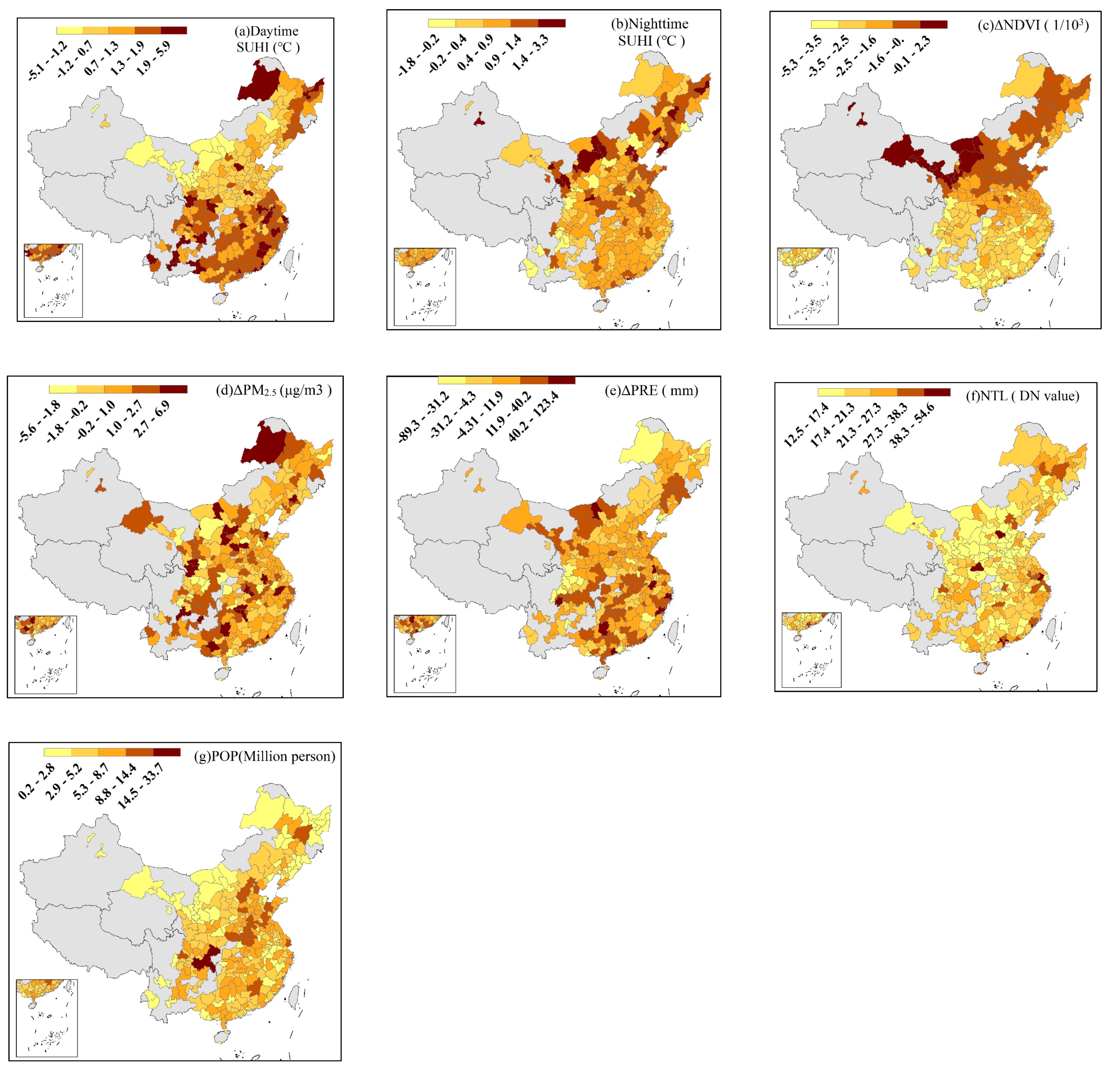
The statistical description and spatial distribution of the variables employed in the estimations are presented in Table 1 and Figure 2, respectively.

3. Methods

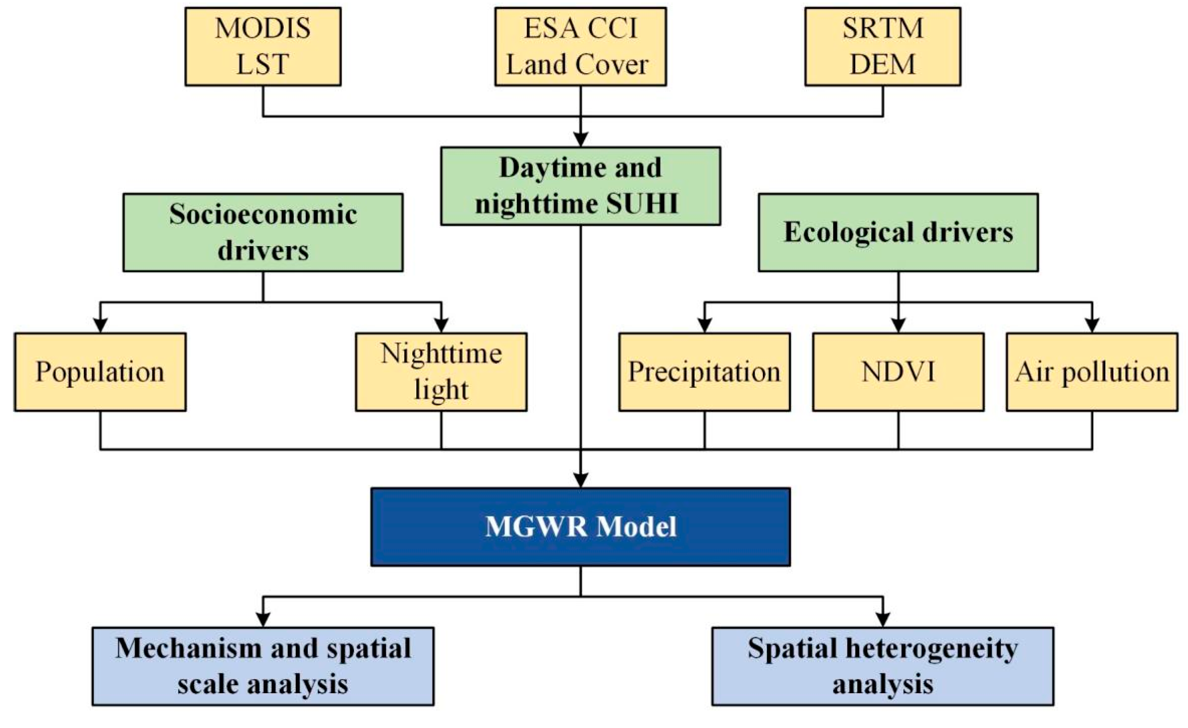
Figure 3 shows the overall framework used in this paper. The first step is SUHI calculation based on multisource remote sensing data, the second step is the construction of the driving factor index system, and the last step is driving factor analysis based on the MGWR model.

3.1. SUHI Intensity Calculation

A large amount of uncertainty in selecting rural references in the SUHI intensity calculations makes it challenging to compare the conclusions of related literature [38,64]. In contrast, taking administrative boundaries (AB) as a rural reference is considered an appropriate SUHI standardized calculation scheme and has been widely used in SUHI studies around the world, including China and the United States [19,65]. The AB method avoids the difference in SUHI intensity due to rural reference buffer delineation and keeps both remotely sensed and socioeconomic data at the same aggregation level. The above two aspects of the AB method illustrate its clear advantages in the analysis of SUHI drivers.
In this study, we delineated urban and rural areas using the ESA CCI land cover data. We first removed certain types of pixels within each city’s administrative borders: the pixels classified as snow and ice and the pixels in extraordinarily high or low positions (pixels with elevations higher or lower than 50 m of the built-up pixel average). Removing such pixels was necessary to eliminate the possible effects of temperature from water bodies and extreme positions. Pixels classified as built-up among the remaining pixels were then flagged as urban areas for each city with its administrative borders. Accordingly, the remaining pixels were referred to as rural areas. After the above processing, we used Equation (1) to calculate the SUHI intensity as follows:
SUHI = U L S T R L S T
where SUHI represents the city’s surface urban heat island intensity, ULST is the average land surface temperature in the urban area, and RLST is the average temperature of the pixels in the rural area. We also processed the three variables NDVI, precipitation, and PM2.5 in the same way to investigate how their differences between urban and rural areas affect SUHIs.

3.2. Ordinary Least Square Model

Typically, linear regression is relatively suitable for describing how a dependent variable is related to several explanatory variables. The equation given below can thus be used to describe an ordinary linear regression model:
Y i = α 0 + k = 1 p α k X i k + ε i , i = 1 , , n
where the dependent variable Y is described by a linear combination of Xk, k = 1, …, p; Ɛi indicates independent error terms, following a zero-mean normal distribution. The OLS is adopted to evaluate the global regression parameters and the multicollinearity of the dataset. The estimated parameters are constant over space during the OLS model calibration process:
α = ( X T X ) 1 X T Y
The MGWR model is then employed for the removal of this constraint.

3.3. Multiscale Geographically Weighted Regression Model

The spatial autocorrelation observed in previous research may be caused by the following: (i) the highly significant regional heterogeneities in China, mainly for coastal and interior areas [66]; (ii) in neighboring regions, the difference between urban climate and environment may be highly significant due to their unique planning pattern and nature. Thus, besides the original global regression method, we take a further step to analyze the relationship between SUHI intensity and several driven factors with the assistance of MGWR, which is an improved method of geographically weighted regression traditionally applied by researchers [67]. MGWR allows different bandwidths (instead of a sole global bandwidth) to be assigned to each variable. The parameters of MGWR are estimated for each observation; thus, the spatially varied correlation between the SUHI intensity and drivers is more exhaustively and intuitively visualized.
When applied to spatial data, a typical linear regression model should assume a relatively stationary process, i.e., when stimuli are the same or similar, the response in each component of the study area will all be the same or similar. However, data that must be applied by spatially variant processing remain where spatial nonstationarity is exhibited. The GWR can be used to overcome this problem and is formulated as follows:
Y i = α 0 ( i ) + k = 1 p α k ( i ) X i k + ε i , i = 1 , , n
Considering that the model parameters are variant across different locations i, then the GWR can be estimated as:
α ( i ) = ( X T W X ( i ) ) 1 X T W ( i ) Y
where W(i) denotes a matrix of weights that is subject to the change of position i (longitude and latitude), considering that the observations closer to i should have more significant weights than distant ones.
In GWR, the data for the current location is estimated based on the neighboring locations. Typically, the weighting matrix can be determined via numerous weighting schemes, although those schemes tend to be Gaussian and reflect the dependency type that usually occurs in most spatial processes. Weighting methods can be categorized into adaptive or fixed approaches. In a fixed Gaussian kernel-based local regression model, the parameter Wij is used to refer to the continuous function for the data location j and local regression location i:
W i j = exp [ ( d i j / h ) 2 2 ]
where dij represents the distance between locations i and j, and h stands for the bandwidth; that is to say, when h grows, the steepness of the kernel gradient reduces, and the local calibration can contain additional data points. The optimum value of h can be derived in the GWR calibration. A choice between variance and bias is required to choose the optimal bandwidth. We obtain the optimal bandwidth via an iterative process in each GWR calibration to minimize the corrected Akaike information criterion (AICC) value.
GWR can capture all spatial heterogeneity in relationships. However, it is assumed that all of these relationships change with a similar spatial scale across any covariate. Since MGWR relaxes the assumption that variables have the same spatial scale and thus makes it possible to optimize the covariate-specific bandwidths, it can improve the GWR significantly. It is formulated as:
log Y i = β b w ( U i , V i ) + j β b w ( U i , V i ) log X i j + ε i
where bw * describes the particular optimum bandwidth employed within the estimation of the * th conditional relationship, while various processes can work at multiple spatial scales using MGWR to respectively derive the bandwidth for certain conditional relationships between the response variable and different predictor ones.
The back-fitting algorithm presented by Fotheringham et al. [34] can be employed to calibrate the MGWR. In this work, MGWR 2.2.1 software was used for calibration (more information can be found at the homepage of MGWR. Available online: https://sgsup.asu.edu/sparc/multiscale-gwr (accessed on 21 October 2021)).

4. Results

4.1. Results of the OLS Analysis

According to the results presented in Table 2, only ΔNDVI and NTL variables always have statistical importance. The coefficients of daytime NTL and Pop and nighttime ΔNDVI, ΔPre, and Pop increase within the study interval, and there is no consistent pattern in the remaining variables’ coefficients. Moreover, the ΔNDVI variable exhibits significant negative orientation in daytime models and positive orientation at nighttime, indicating that, in the global model, the control of SUHIs by vegetation shows opposite patterns during the day and night, i.e., ΔNDVI mitigates urban heat islands during the day and exacerbates them at night. In contrast, the NTL and Pop variables have a positive orientation in both daytime and nighttime models, indicating that the socioeconomic conditions of the city always increase SUHIs. Pre and PM2.5 variables do not exhibit stable driving patterns over the study period, indicating that climate and air pollution factors influence SUHIs in complex ways, and an accurate conclusion is difficult to obtain. However, the above two points are likely inaccurate conclusions due to the global model’s inability to capture the heterogeneity of spatial context and geographic locations.
For diagnostic information, the R2 of the daytime model is significantly higher than that of the nighttime. The highest R2 is acquired from the daytime 2015 data (0.666), and the lowest R2 is observed in the nighttime 2005 data (0.087). Thus, the daytime OLS models have reasonable R2 values. However, a direct comparison of AICc among different models with various datasets is of little necessity. Therefore, RSS and AICc are taken for comparison with the MGWR model for improvement. We employ the distribution of OLS standard residuals in Figures S1 and S2 to obtain a primary observation of the spatial autocorrelation. The residual maps show that high standard residuals exist in many municipalities, while their corresponding distributions are relatively clustered within the years 2005, 2010, 2015, and 2018. A multicollinearity test is also performed with variance inflation factor (VIF) numbers as the diagnostic data to determine multicollinearity. A relatively ideal value of the VIF for a predictor variable cannot be greater than 10. For every model, the VIFs are all below 2, which means there is no significant multicollinearity between variables.
In addition to these analyses, Moran’s criterion for all three time periods (see Table 3) is utilized to verify the existence of spatial autocorrelation in the SUHIs. The test results indicate that SUHI intensities in this study have a likelihood lower than 1% (p-value < 0.01) in all years, demonstrating a significant spatial autocorrelation of SUHI intensity. Combined with the maps of residual distribution, the clustered patterns can be generated randomly, indicating significant spatial heterogeneity in the OLS model.

4.2. MGWR Results

The dependent and independent variables of the MGWR model are similar to those employed by the OLS model. Local model results are presented in Tables S1–S4. Comparing the diagnostic data of the OLS results, the MGWR model achieves superior efficiency considering its lower RSS and AICc values and its higher regulated R2. This enhancement is more significant in the nighttime than in the daytime. Furthermore, the MGWR models can allocate various bandwidths for variables. Thus, the bandwidths are changed according to the variables (see Tables S1–S4).
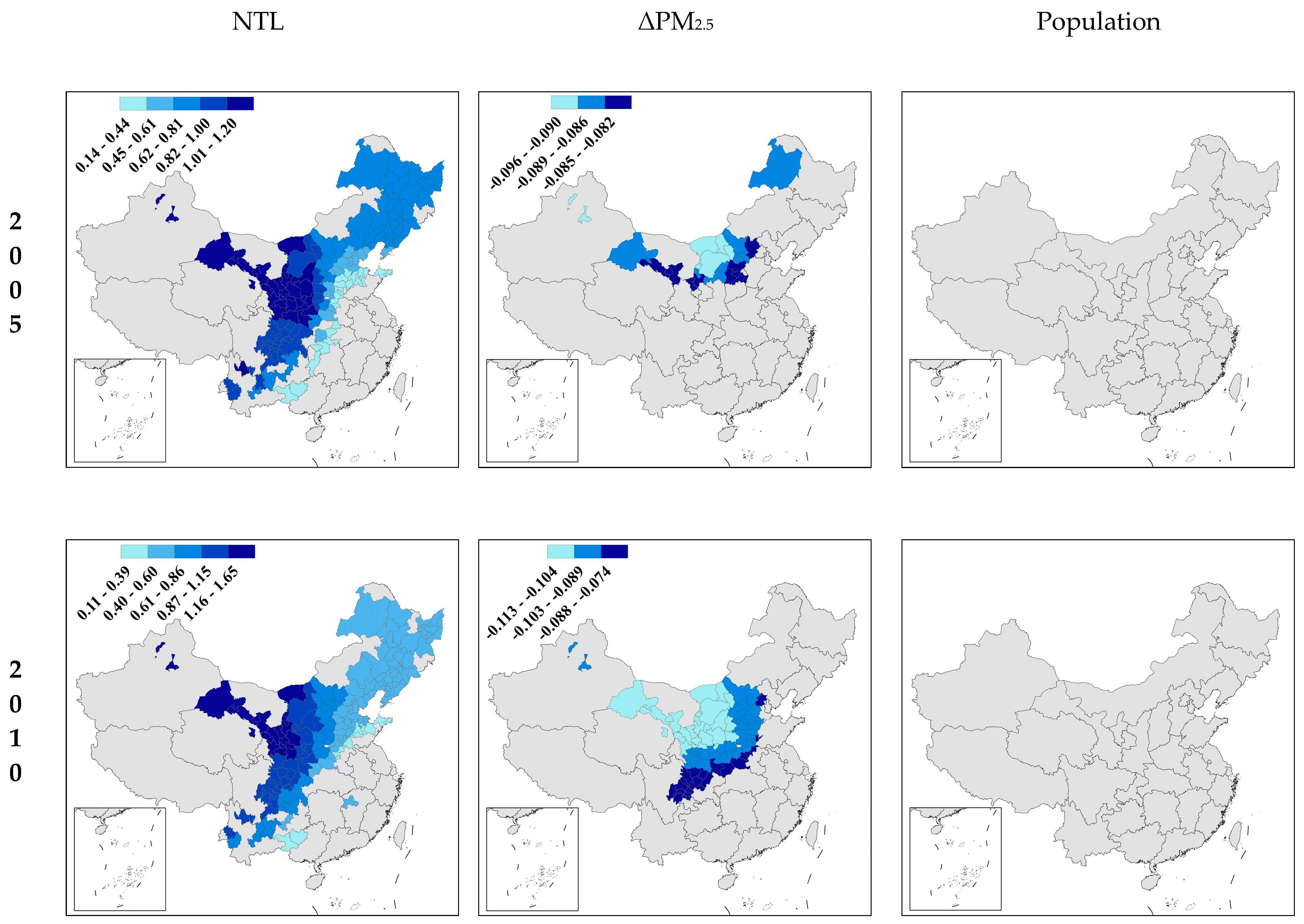
Both ΔPM2.5 and Pop can be considered as global variables (bandwidths are between 252–281), which means they control SUHIs in the same way globally. However, the remaining four variables show significant spatial variations (bandwidths are between 43 and 124), further illustrating the necessity of applying the MGWR model. The bandwidths of the vast majority of variables in the nighttime model are typically larger than those in the daytime, suggesting that the spatial heterogeneity of daytime SUHI drivers is stronger than that of the nighttime. While spatial data and spatial processes are two different concepts, in this study, they display a similar spatial heterogeneity pattern (daytime greater than nighttime).
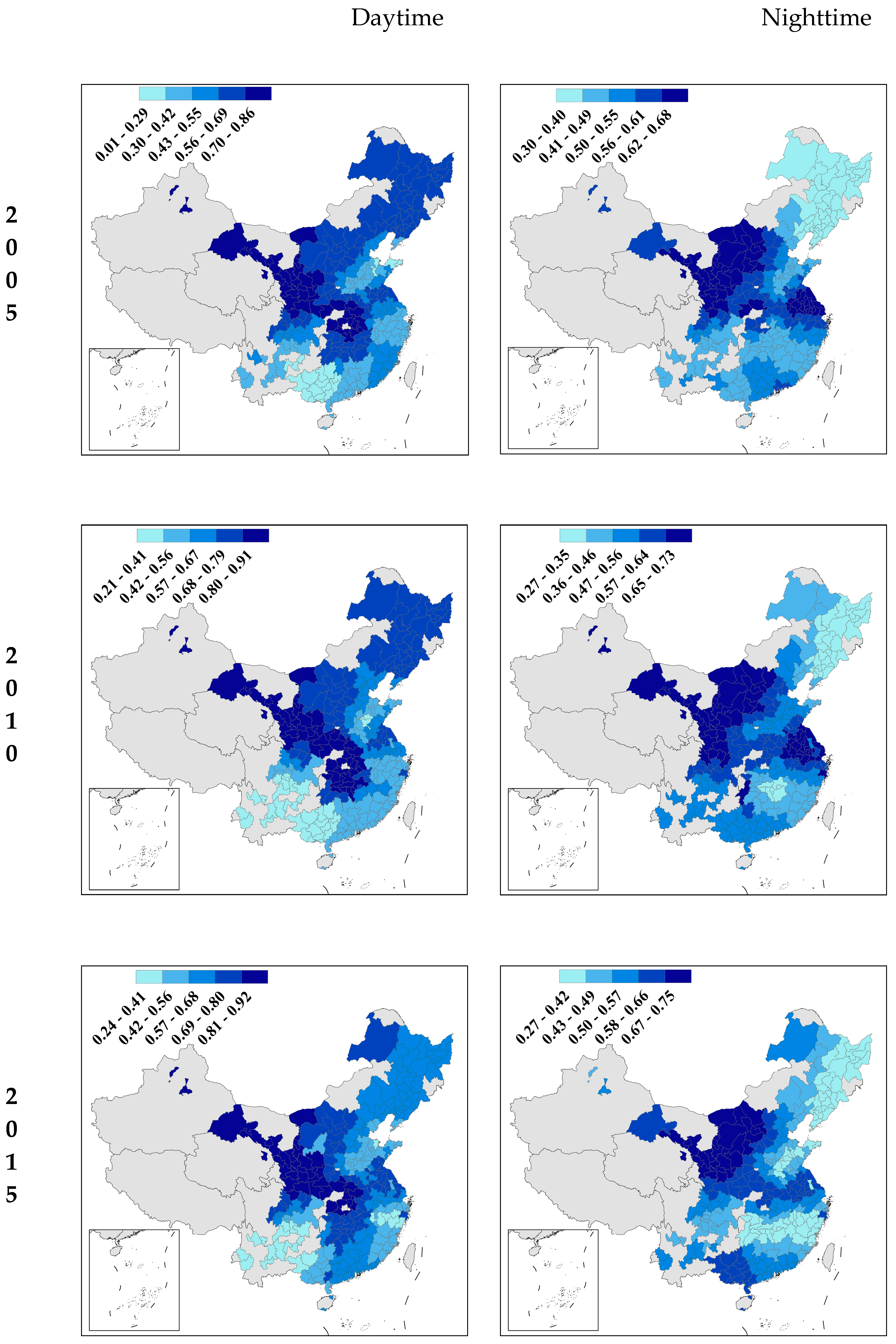
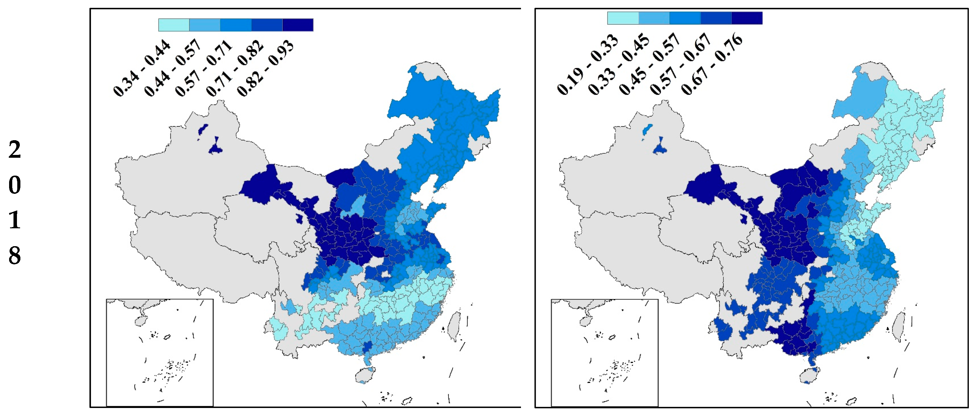
Figure 4 shows the variations of local R2 distribution in the analyzed duration. A higher local R2 for a city indicates a higher explainable level of correlation. The relatively lower R2 are usually localized in the Southwest region in the daytime and are concentrated in the Northeast at night. From 2005 to 2018, the spatiotemporal distribution pattern of R2 does not change much, but the explanation rate of the model increases. This result indicates that the explanatory variables selected in this paper cover the main drivers of SUHIs, which become increasingly important as a city expands. The comprehensive parameters leading to the mentioned variations are presented subsequently.
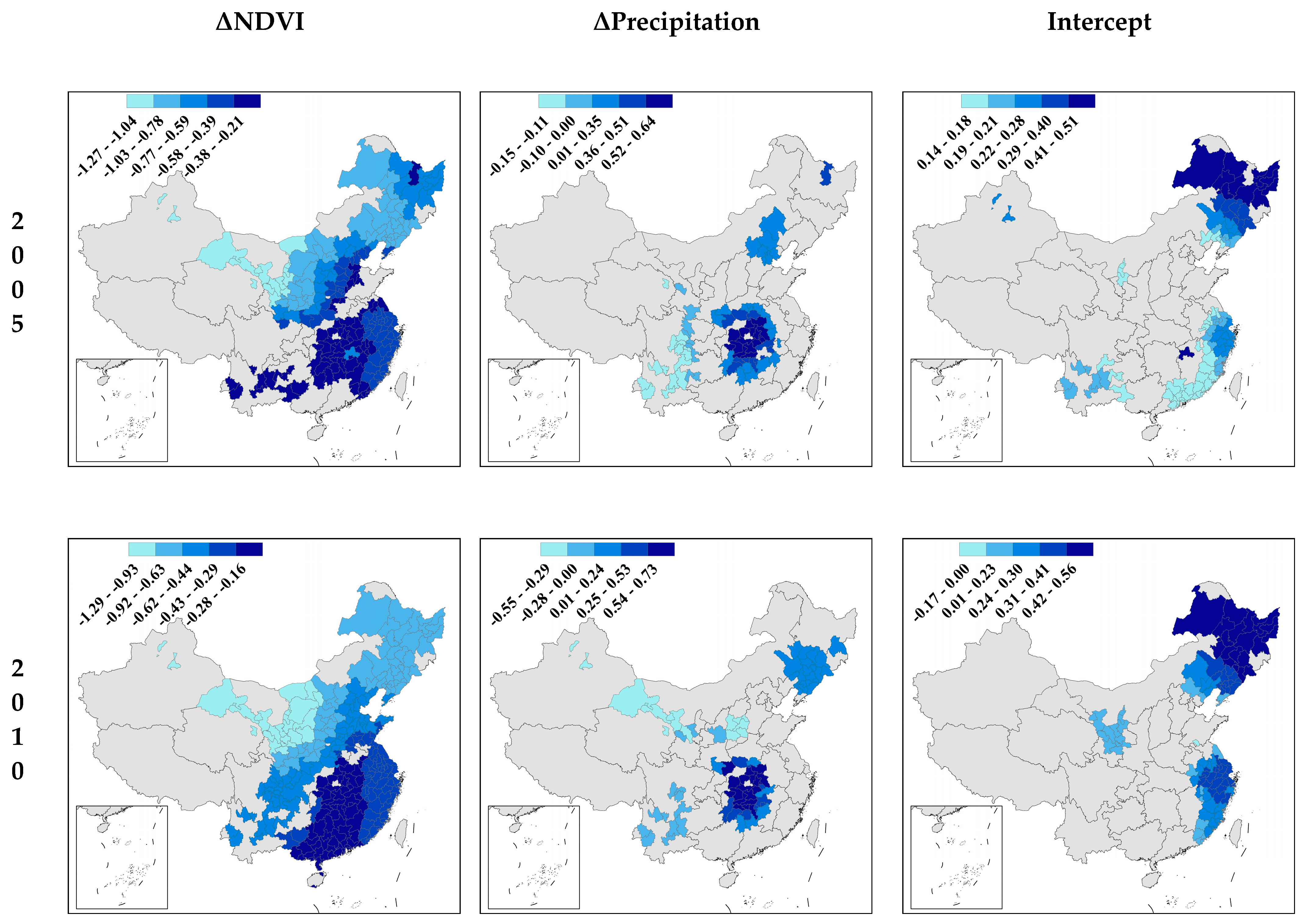
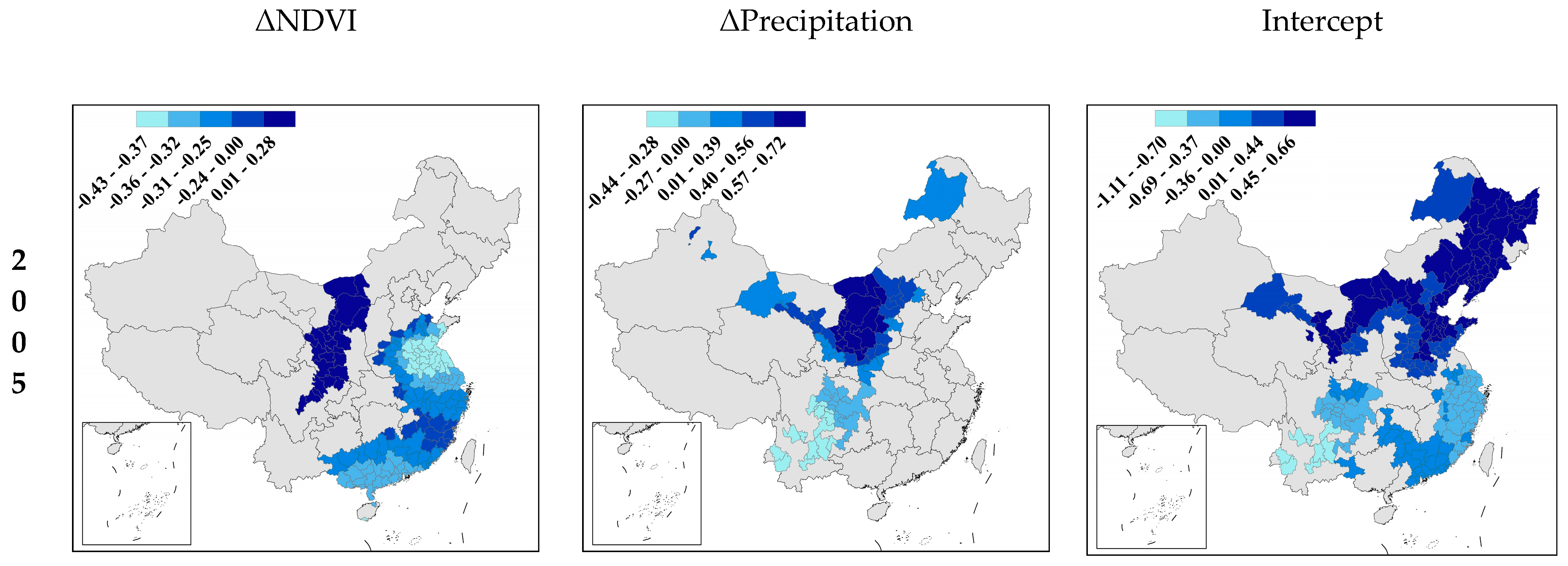
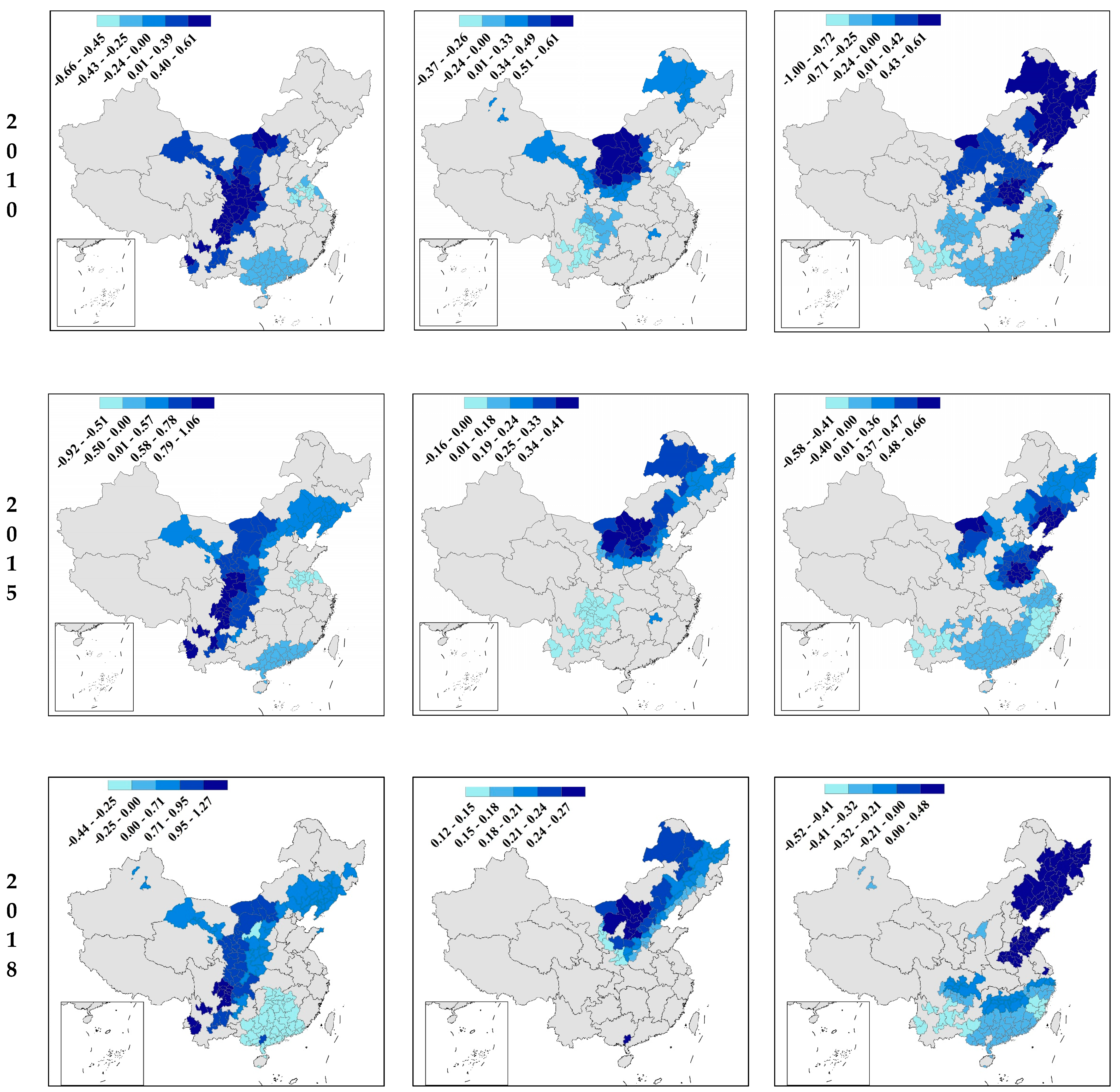
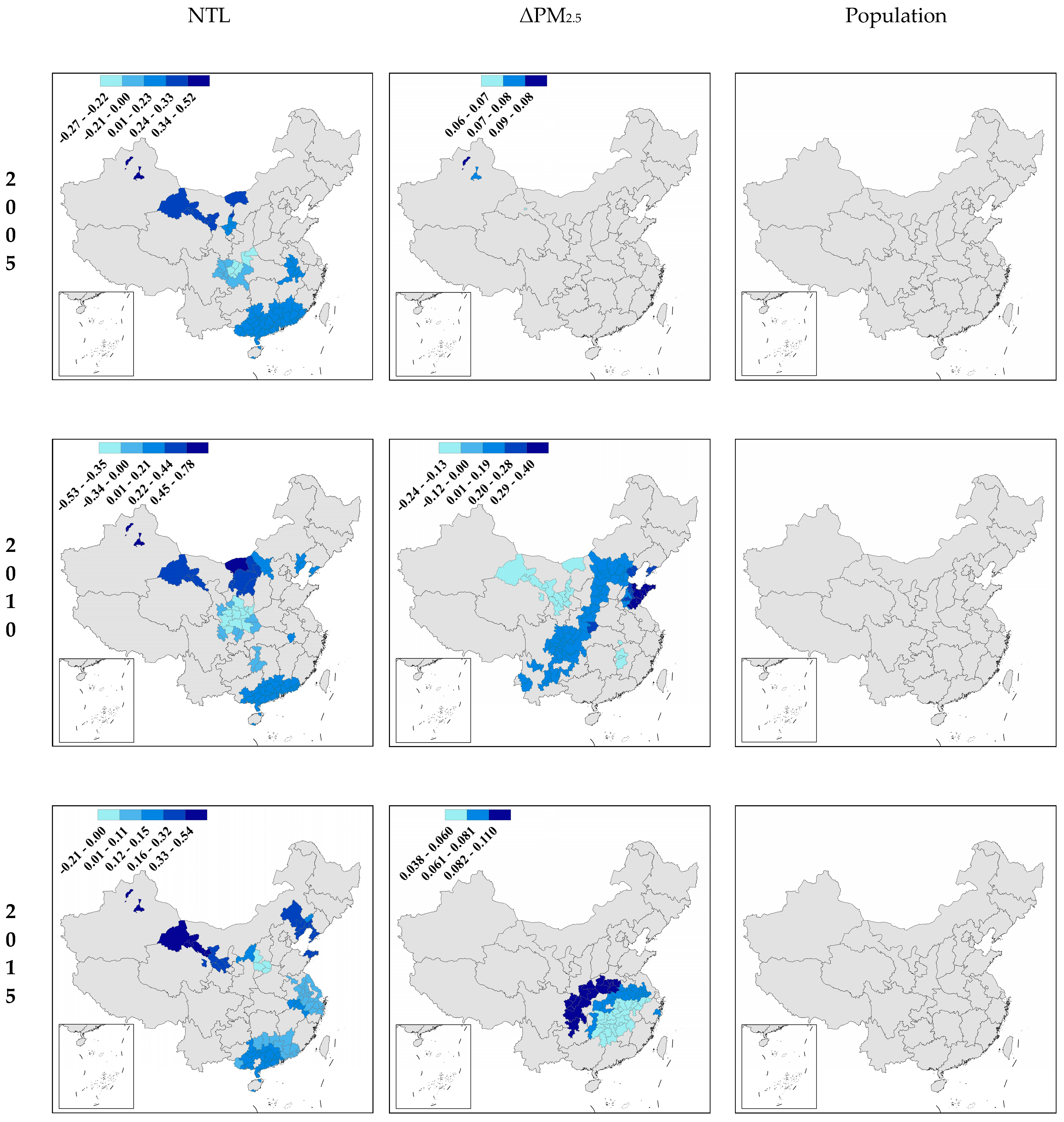
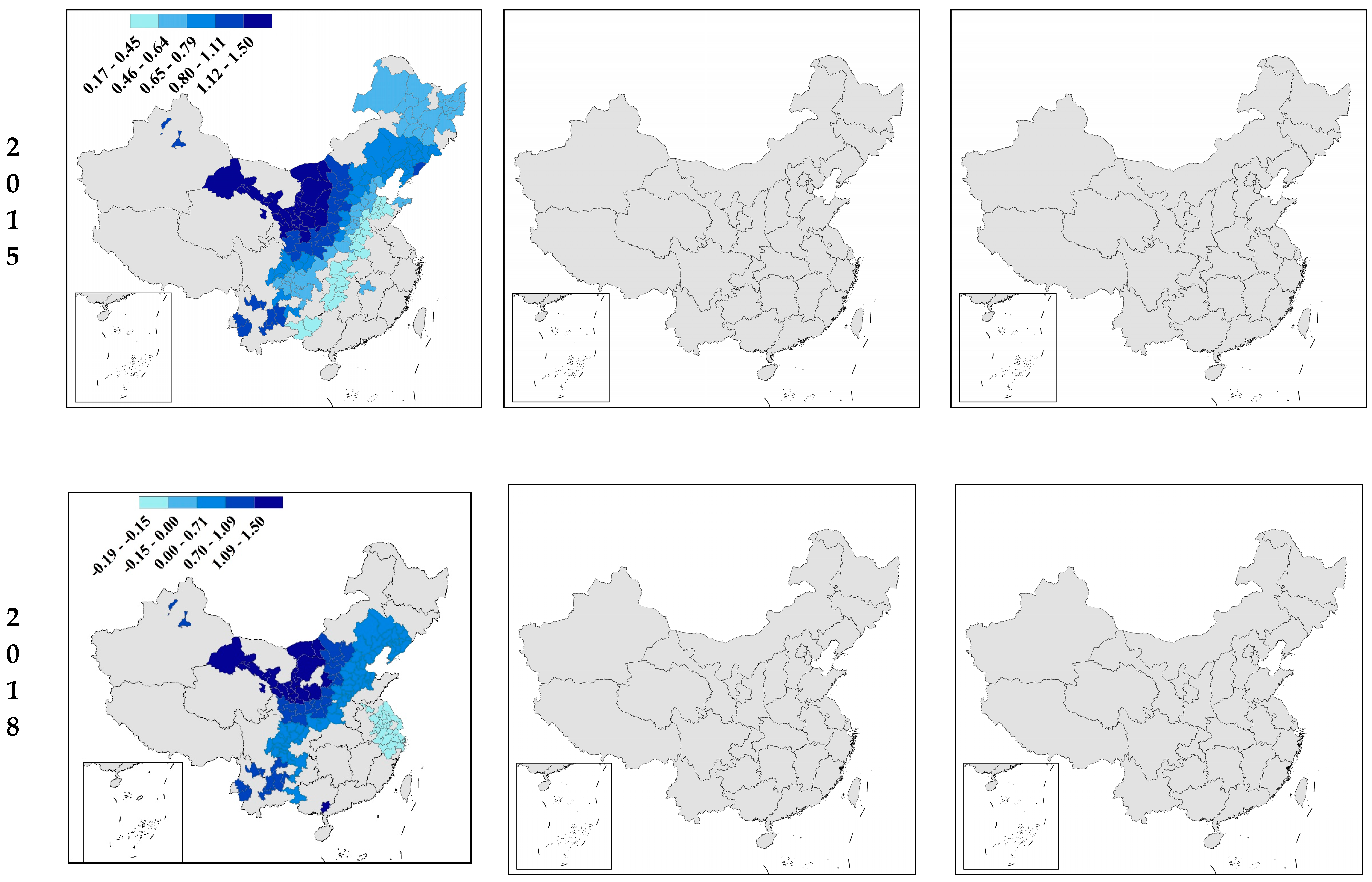
Figure 5, Figure 6, Figure 7 and Figure 8 show the change of local significance and the variable’s coefficients from 2005 to 2018. Only the municipalities with a notable dependency between SUHIs and variables are colored (p-value < 0.1). Various patterns and characteristics can be determined from the results, including: (i) Figure 5 and Figure 6 show that the daytime ΔNDVI variable’s coefficient is negative in all cities. Still, the effect is generally higher in the Northwest than in the Southeast. Conversely, the nighttime situation produces significant differences, with largely negative coefficients in the Southeast and positive coefficients in the Northwest. This suggests that the control of SUHIs by vegetation indeed differs considerably between the day and night but differently from the coarse pattern expressed by the global model (i.e., the OLS model). Since vegetation is the most crucial driver of SUHIs, it is discussed further in Section 5.2. (ii) As also illustrated in Figure 5 and Figure 6, the effect of the ΔPre variable on SUHIs is positive in the Northwest, both during the night and day. Apart from this, there is a strongly negative effect in the central region during the daytime and in the North during the nighttime. This revealed that there was a strong spatial heterogeneity in the impact of precipitation on SUHI. (iii) In addition, Figure 5 and Figure 6 demonstrate the influence of spatial context on SUHIs. Along with the covariate-specific optimized bandwidths, the intercept’s local estimates are perhaps the most compelling output from the MGWR. These indicate the intrinsic levels of the dependent variable holding everything else in the model constant. In this case, the local intercept estimates indicate the inherent impact of cities on SUHIs. In essence, this is a measure of spatial context. The spatial context may include some urban features that are difficult to quantify on a large scale, including the architectural style or drainage structure of the city itself. The effect of spatial context on SUHIs is significantly positive only in the Northeast and Southeast during the daytime and nighttime. At night, the regional extent of the effect increases significantly and is positive in the North and negative in the South. (iv) Air pollution has often been considered a critical SUHI driver in previous studies. However, according to Figure 7 and Figure 8, air pollution does not appear to have a significant influence, particularly in 2015 and 2018. This result may be related to a series of public strategies (such as the Air Pollution Prevention and Control Action Plan) enacted by the Chinese government targeting PM2.5 reduction. (v) The NTL and Pop variables together characterize the city’s socioeconomic level. Interestingly, the Pop variable is insignificant in almost all models, and the effect of NTL on SUHIs differs significantly between daytime and nighttime.

5. Discussion

5.1. Multiscale Extensions of Geographically Weighted Regression

The respective bandwidths produced by MGWR can more intuitively interpret geographical scale [34]. MGWR could also enhance policy-making by framing UHI determinants using a possible combination of global, regional, and local spatial contexts.
Several past studies have investigated the drivers of urban heat islands using classical GWR models [44,45,46], which inevitably ignore the fact that different relationships may occur at different scales. To address this issue, we analyze the same variables utilized in the GWR model to compare the differences between the GWR and MGWR models (Table 4).
Results indicate that the GWR bandwidth can be considered an intermediate value of the MGWR bandwidth, i.e., it ignores the global robustness of some variables and fails to capture the spatial heterogeneity of some variables. Thus, GWR models typically have lower R2 and higher AICC and RSS than MGWR models and produce specific local parameters that are difficult to interpret. For example, the results of MGWR’s analysis show that the effect of vegetation on SUHIs is very localized (bandwidths are small) compared to air pollution, and the development of UHI mitigation policies from these two perspectives should focus on inter-regional characteristics.
It is worth noting that previous studies usually mention that MGWR models can better handle the problem of multicollinearity. However, all models in this study do not have significant multicollinearity (VIF < 1.5 in the OLS model, local condition index < 15 in MGWR and GWR models, see Table S5). There is no discussion of multicollinearity in the different models.

5.2. Seasonal Variation of SUHIs and Vegetation

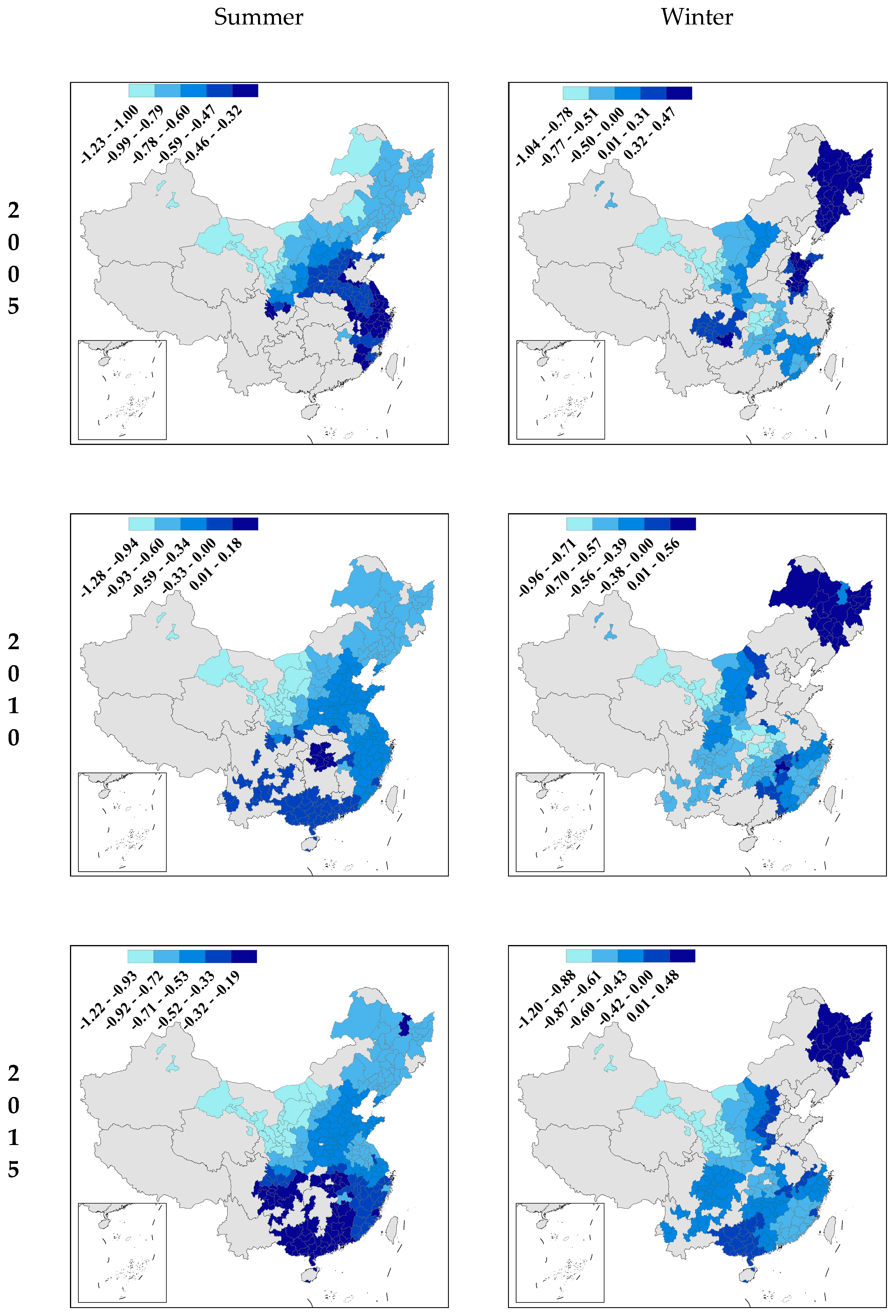
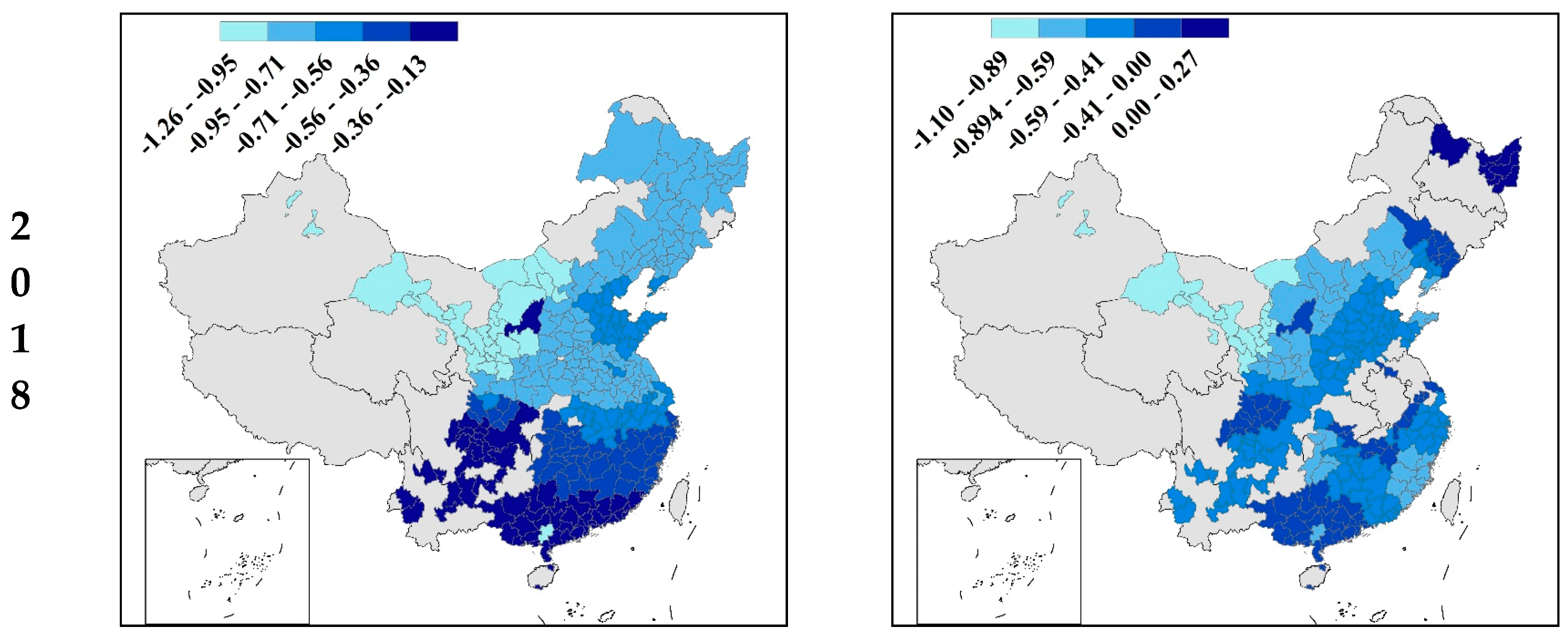
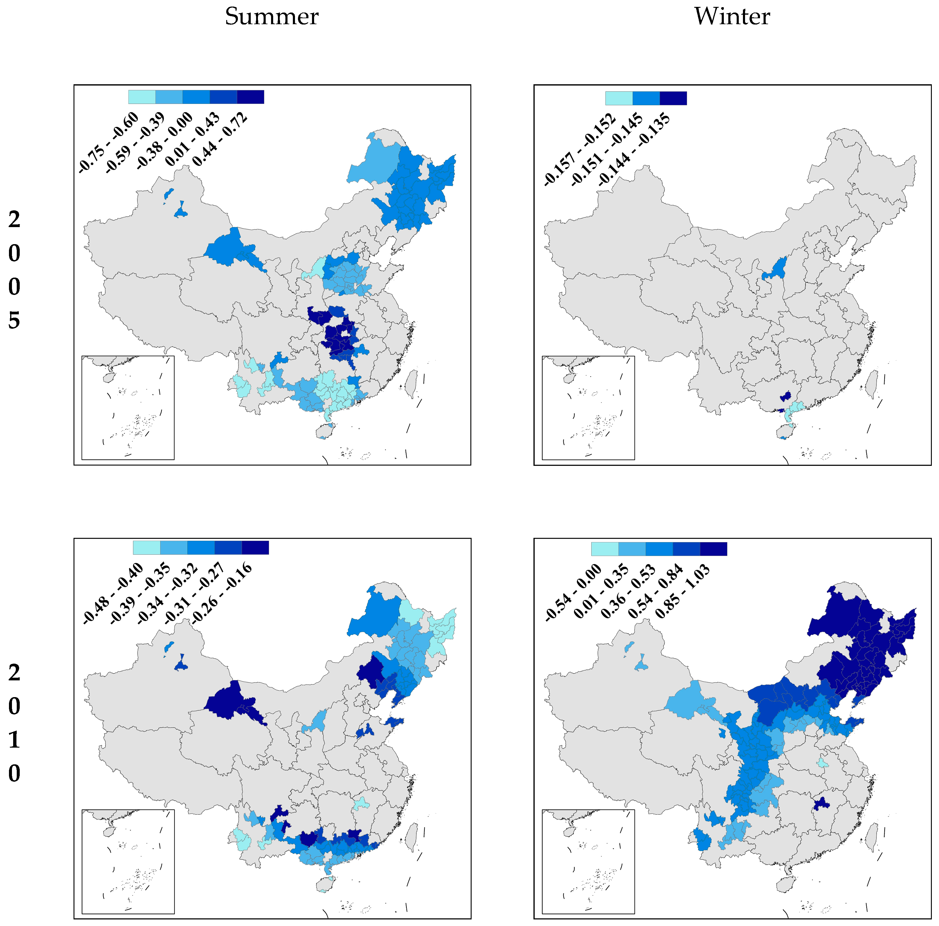
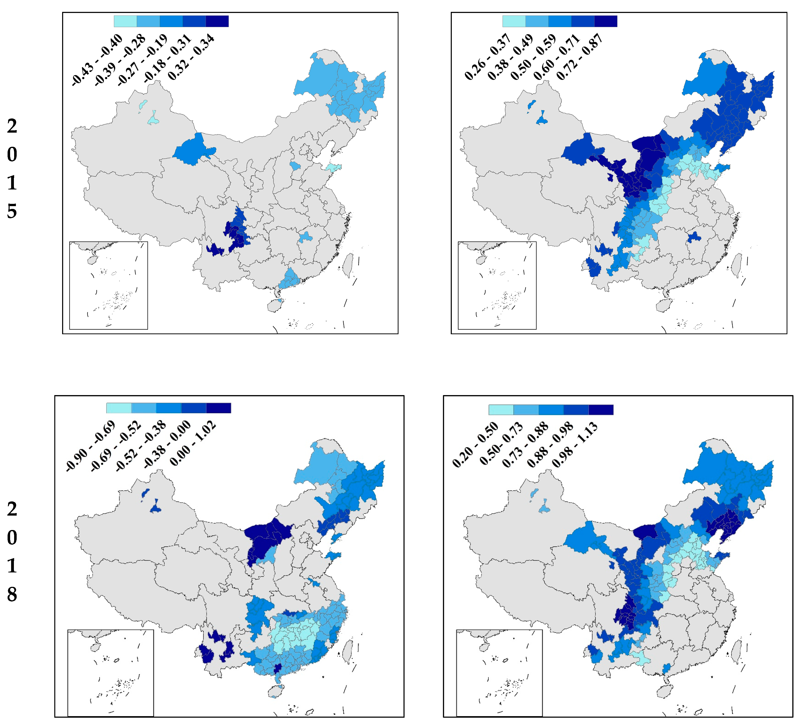
In all models used in this study, vegetation differences among urban and rural areas are the most critical drivers of SUHIs, and previous studies have come to a similar conclusion [14,20,30,53]. However, in the present study, in some areas, larger ΔNDVI increases SUHIs at night. This phenomenon seems to contradict the classical theory that “vegetation is a regulator of urban temperature” [68]. The areas with positive ΔNDVI effects on nighttime urban heat islands are concentrated in China’s most economically dynamic Shenzhen metropolitan region. In contrast, those with negative effects are concentrated in the less economically developed Northwest region. The significant socioeconomic and climatic differences between the two areas result in significantly different vegetation types. The Shenzhen metropolitan region has a substantially higher proportion of artificial vegetation than the Northwest. Therefore, we speculate that the difference in vegetation types may affect how vegetation controls SUHIs to some extent. To further test this hypothesis, we keep the remaining variables inconvenient and analyze the relationship between SUHI and ΔNDVI in summer and winter, respectively, using the MGWR model (Figure 9 and Figure 10).
Results show that the contribution of ΔNDVI to SUHIs is negative in almost all cities during the summer daytime and negative during the winter daytime except for in the Northeast area. During summer nights, the coefficient of ΔNDVI remains positive in the GBA region, while it is mainly negative in the rest of the region. Most interestingly, during winter nights, the coefficients of ΔNDVI are primarily positive across the country and are significant only in the Northwest, Northeast, and Southwest regions (except for in 2005). The above results suggest that differences in vegetation type may indeed lead to changes in the mechanism of vegetation influence on nighttime SUHIs and that such changes are more likely to occur in summer.

5.3. Spatial Context and Population

Unlike the global mode, the MGWR does not statistically intercept at zero, and the spatial heterogeneity identifies hot spots of SUHIs in the parameter estimates after the applied variables have been controlled. Both geographical effects associated with the remaining and omitted variables may be included in these spatial patterns. For instance, spatial context may make a noticeable contribution to the city’s architectural style, the consumption structures of residents and further alter the thermal environment of the city. Alternatively, the intercept may help in policy formation, informing follow-up investigations and additional determinants. For example, in this study, the effects of intercept variables on SUHIs are all positive during the daytime and positive in the North and negative in the South in the nighttime. This result indicates that urban characteristics, such as latitude, architecture, and urban planning, significantly affect nighttime north–south SUHIs. Further research on these findings is essential for the mitigation of nighttime SUHIs.
The MGWR has another advantage in exploring the robustness of abstractions applied in the definition of explanatory variables. While population variables have received extensive attention in previous studies [30,40], no statistically nonzero local associations with SUHIs are observed in our study. Comparing this study to prior studies reveals that the effect of population indicators on SUHI may not be robust. This implies that more indicators of drivers need to be developed in the study of SUHIs to obtain more meaningful analysis results. For example, more appropriate indicators to characterize the impact of human activities on the urban thermal environment should be considered rather than simply employing the population within an administrative boundary as the indicator.

6. Conclusions

While previous studies have examined the drivers of SUHIs in detail using multiple temporal and spatial dimensions, driver spatial heterogeneity and spatial scale have received little attention. This study provided a comprehensive and in-depth analysis of SUHIs in China for 2005, 2010, 2015, and 2018 using the MGWR model. According to the obtained results, the MGWR model outperformed the OLS and classical GWR models in terms of both diagnostic indicators and model coefficient interpretability. The MGWR model had significantly enhanced explanatory power during the daytime than during the nighttime, with ΔNDVI and NTL variables being the most important during the daytime and nighttime, respectively. The control pattern of vegetation on SUHIs was significantly different at night, and even positive effects were observed in Northwest and Northeast regions. By further analyzing the seasonal variability of vegetation and SUHIs, we found that differences in vegetation types due to socioeconomic and urban development patterns may be the main reason for spatial heterogeneity as the driving force of vegetation on SUHIs.
This paper also provided some potential references for the development of regionally targeted SUHI mitigation policies. For example, the results from the MGWR model suggested that air pollution management is also of considerable value in improving the thermal environment of urban agglomerations in North and Central China. In addition, the increase of vegetation in urban areas played an essential role in urban environmental management in the daytime in northern regions and during the night in southern areas. According to the analysis of the influence patterns of spatial context on SUHIs, managing the urban thermal environment at night was much more challenging than vegetation planting and air pollution controls in the daytime, especially in eastern China. From the spatial scale of drivers, a joint prevention and control approach should be adopted to manage air pollution and thus mitigate SUHI because PM2.5 as a global variable has a widespread effect on SUHIs. The mitigation of SUHIs through the control of other local variables requires a more tailored approach. Furthermore, because China covers various climate zones, our research has a specific global reference value.
We acknowledge that the relevant conclusions of this study are confined to obvious sky situations. The MGWR model in this study explains 62% (nighttime) to 87% (daytime) of the inter-regional variations in SUHI intensity. However, despite its excellent performance, the inevitable problem of omitted variables remains in the present model, which is largely due to variable measurements. For example, urban drainage structures may affect SUHIs by changing urban evapotranspiration, but it is challenging to find a suitable and accurate indicator to quantify it. It will also be valuable to add more driving factors and extend the research time (for example, combining simulation data to quantify future SUHIs under multiple scenarios) in future research.
Nevertheless, the current work provides valuable insights into the attribution analysis of SUHIs by systematically investigating the spatiotemporal patterns of SUHI driving factors from a multiscale perspective. Accordingly, it provides a full explanation and realization of SUHIs and references for developing urban environmental governance policies.

Supplementary Materials

The following are available online at https://www.mdpi.com/article/10.3390/rs13214428/s1, Figure S1: Spatial distributions of standard residuals of daytime OLS regression and MGWR model in 2005; Figure S2: Spatial distributions of standard residuals of nighttime OLS regression and MGWR model in 2005; Table S1. Results of multiscale geographically weighted regression model between SUHI intensity and drivers in 2005; Table S2. Results of multiscale geographically weighted regression model between SUHI intensity and its drivers in 2010; Table S3. Results of multiscale geographically weighted regression model between SUHI intensity and drivers in 2015; Table S4. Results of multiscale geographically weighted regression model between SUHI intensity and drivers in 2018; Table S5. Local condition index of each city in MGWR mode (take daytime 2015 as an example).

Author Contributions

Conceptualization, L.N. and Z.Z.; methodology, L.N.; software, L.N.; validation, Y.L.; formal analysis, Z.P.; data curation, J.W.; writing—original draft preparation, L.N.; writing—review and editing, M.L.; visualization, Y.J.; supervision, Z.Z. and R.T.; project administration, Z.Z.; funding acquisition, Z.Z. All authors have read and agreed to the published version of the manuscript.

Funding

This work is supported by the National Natural Science Foundation of China (Grant Nos. 42077433 and 71874196), the Fundamental Research Funds for the Central Universities, and the Research Funds of Renmin University of China (Project No. 21XNH037).

Data Availability Statement

The data are freely available upon request.

Conflicts of Interest

The authors declare no conflict of interest.

References

  1. Zhou, L.; Dickinson, R.E.; Tian, Y.; Fang, J.; Li, Q.; Kaufmann, R.K.; Tucker, C.J.; Myneni, R.B. Evidence for a significant urbanization effect on climate in China. Proc. Natl. Acad. Sci. USA 2004, 101, 9540–9544. [Google Scholar] [CrossRef] [Green Version]
  2. Kalnay, E.; Cai, M. Impact of urbanization and land-use change on climate. Nature 2003, 423, 528–531. [Google Scholar] [CrossRef]
  3. Deng, J.S.; Wang, K.; Hong, Y.; Qi, J.G. Spatio-temporal dynamics and evolution of land use change and landscape pattern in response to rapid urbanization. Landsc. Urban Plan. 2009, 92, 187–198. [Google Scholar] [CrossRef]
  4. Oke, T.R. City size and the urban heat island. Atmos. Environ. 1973, 7, 769–779. [Google Scholar] [CrossRef]
  5. Howard, L. Climate of London deduced from meteorological observation. Harvey Darton 1833, 1, 1–24. [Google Scholar]
  6. Kolokotroni, M.; Ren, X.; Davies, M.; Mavrogianni, A. London’s urban heat island: Impact on current and future energy consumption in office buildings. Energy Build. 2012, 47, 302–311. [Google Scholar] [CrossRef] [Green Version]
  7. Kikegawa, Y.; Genchi, Y.; Kondo, H.; Hanaki, K. Impacts of city-block-scale countermeasures against urban heat-island phenomena upon a building’s energy-consumption for air-conditioning. Appl. Energy 2006, 83, 649–668. [Google Scholar] [CrossRef]
  8. Parker, J. The Leeds urban heat island and its implications for energy use and thermal comfort. Energy Build. 2021, 235, 110636. [Google Scholar] [CrossRef]
  9. Sarrat, C.; Lemonsu, A.; Masson, V.; Guedalia, D. Impact of urban heat island on regional atmospheric pollution. Atmos. Environ. 2006, 40, 1743–1758. [Google Scholar] [CrossRef]
  10. Li, H.; Meier, F.; Lee, X.; Chakraborty, T.; Liu, J.; Schaap, M.; Sodoudi, S. Interaction between urban heat island and urban pollution island during summer in Berlin. Sci. Total Environ. 2018, 636, 818–828. [Google Scholar] [CrossRef] [PubMed]
  11. Čeplová, N.; Kalusová, V.; Lososová, Z. Effects of settlement size, urban heat island and habitat type on urban plant biodiversity. Landsc. Urban Plan. 2017, 159, 15–22. [Google Scholar] [CrossRef]
  12. Géron, C.; Lembrechts, J.J.; Nijs, I.; Monty, A. Shielded environments reduce stress in alien Asteraceae species during hot and dry summers along urban-to-rural gradients. Ecol. Evol. 2021, 11, 10613–10626. [Google Scholar] [CrossRef]
  13. Tan, J.; Zheng, Y.; Tang, X.; Guo, C.; Li, L.; Song, G.; Zhen, X.; Yuan, D.; Kalkstein, A.J.; Li, F. The urban heat island and its impact on heat waves and human health in Shanghai. Int. J. Biometeorol. 2010, 54, 75–84. [Google Scholar] [CrossRef]
  14. Goggins, W.B.; Chan, E.Y.; Ng, E.; Ren, C.; Chen, L. Effect modification of the association between short-term meteorological factors and mortality by urban heat islands in Hong Kong. PLoS ONE 2012, 7, e38551. [Google Scholar]
  15. He, B.-J.; Wang, J.; Liu, H.; Ulpiani, G. Localized synergies between heat waves and urban heat islands: Implications on human thermal comfort and urban heat management. Environ. Res. 2021, 193, 110584. [Google Scholar] [CrossRef]
  16. Oke, T.R. The energetic basis of the urban heat island. Q. J. R. Meteorol. Soc. 1982, 108, 1–24. [Google Scholar] [CrossRef]
  17. Stewart, I.; Mills, G. The Urban Heat Island: A Guidebook; Elsevier: Amsterdam, The Netherlands, 2021. [Google Scholar]
  18. Clinton, N.; Gong, P. MODIS detected surface urban heat islands and sinks: Global locations and controls. Remote Sens. Environ. 2013, 134, 294–304. [Google Scholar] [CrossRef]
  19. Lai, J.; Zhan, W.; Huang, F.; Voogt, J.; Bechtel, B.; Allen, M.; Peng, S.; Hong, F.; Liu, Y.; Du, P. Identification of typical diurnal patterns for clear-sky climatology of surface urban heat islands. Remote Sens. Environ. 2018, 217, 203–220. [Google Scholar] [CrossRef]
  20. Runnalls, K.; Oke, T. Dynamics and controls of the near-surface heat island of Vancouver, British Columbia. Phys. Geogr. 2000, 21, 283–304. [Google Scholar] [CrossRef]
  21. De Faria Peres, L.; de Lucena, A.J.; Rotunno Filho, O.C.; de Almeida França, J.R. The urban heat island in Rio de Janeiro, Brazil, in the last 30 years using remote sensing data. Int. J. Appl. Earth Obs. Geoinf. 2018, 64, 104–116. [Google Scholar] [CrossRef]
  22. Imhoff, M.L.; Zhang, P.; Wolfe, R.E.; Bounoua, L. Remote sensing of the urban heat island effect across biomes in the continental USA. Remote Sens. Environ. 2010, 114, 504–513. [Google Scholar] [CrossRef] [Green Version]
  23. Schwarz, N.; Lautenbach, S.; Seppelt, R. Exploring indicators for quantifying surface urban heat islands of European cities with MODIS land surface temperatures. Remote Sens. Environ. 2011, 115, 3175–3186. [Google Scholar] [CrossRef]
  24. Bhang, K.J.; Park, S.-S. Evaluation of the surface temperature variation with surface settings on the urban heat island in Seoul, Korea, using Landsat-7 ETM+ and SPOT. IEEE Geosci. Remote Sens. Lett. 2009, 6, 708–712. [Google Scholar] [CrossRef]
  25. Khamchiangta, D.; Dhakal, S. Physical and non-physical factors driving urban heat island: Case of Bangkok Metropolitan Administration, Thailand. J. Environ. Manag. 2019, 248, 109285. [Google Scholar] [CrossRef] [PubMed]
  26. Stewart, I.D.; Oke, T.R. Local climate zones for urban temperature studies. Bull. Am. Meteorol. Soc. 2012, 93, 1879–1900. [Google Scholar] [CrossRef]
  27. Li, Z.-L.; Si, M.; Leng, P. A Review of Remotely Sensed Surface Urban Heat Islands from the Fresh Perspective of Comparisons Among Different Regions (Invited Review). Prog. Electromagn. Res. C 2020, 102, 31–46. [Google Scholar] [CrossRef]
  28. Peng, S.; Piao, S.; Ciais, P.; Friedlingstein, P.; Ottle, C.; Bréon, F.-M.; Nan, H.; Zhou, L.; Myneni, R.B. Surface Urban Heat Island Across 419 Global Big Cities. Environ. Sci. Technol. 2012, 46, 696–703. [Google Scholar] [CrossRef]
  29. Zhao, L.; Lee, X.; Smith, R.B.; Oleson, K. Strong contributions of local background climate to urban heat islands. Nature 2014, 511, 216–219. [Google Scholar] [CrossRef]
  30. Manoli, G.; Fatichi, S.; Schläpfer, M.; Yu, K.; Crowther, T.W.; Meili, N.; Burlando, P.; Katul, G.G.; Bou-Zeid, E. Magnitude of urban heat islands largely explained by climate and population. Nature 2019, 573, 55–60. [Google Scholar] [CrossRef]
  31. Priyankara, P.; Ranagalage, M.; Dissanayake, D.; Morimoto, T.; Murayama, Y. Spatial process of surface urban heat island in rapidly growing Seoul metropolitan area for sustainable urban planning using Landsat data (1996–2017). Climate 2019, 7, 110. [Google Scholar] [CrossRef] [Green Version]
  32. Moellering, H.; Tobler, W. Geographical variances. Geogr. Anal. 1972, 4, 34–50. [Google Scholar] [CrossRef]
  33. Liverman, D. Who governs, at what scale and at what price? Geography, environmental governance, and the commodification of nature. Ann. Assoc. Am. Geogr. 2004, 94, 734–738. [Google Scholar]
  34. Fotheringham, A.S.; Yang, W.; Kang, W. Multiscale geographically weighted regression (MGWR). Ann. Am. Assoc. Geogr. 2017, 107, 1247–1265. [Google Scholar] [CrossRef]
  35. Yang, Q.; Huang, X.; Li, J. Assessing the relationship between surface urban heat islands and landscape patterns across climatic zones in China. Sci. Rep. 2017, 7, 1–11. [Google Scholar] [CrossRef]
  36. Zhou, D.; Zhao, S.; Zhang, L.; Liu, S. Remotely sensed assessment of urbanization effects on vegetation phenology in China’s 32 major cities. Remote Sens. Environ. 2016, 176, 272–281. [Google Scholar] [CrossRef] [Green Version]
  37. Sun, R.; Lü, Y.; Yang, X.; Chen, L. Understanding the variability of urban heat islands from local background climate and urbanization. J. Clean. Prod. 2019, 208, 743–752. [Google Scholar] [CrossRef]
  38. Niu, L.; Tang, R.; Jiang, Y.; Zhou, X. Spatiotemporal patterns and drivers of the surface urban heat island in 36 major cities in China: A comparison of two different methods for delineating rural areas. Sustainability 2020, 12, 478. [Google Scholar] [CrossRef] [Green Version]
  39. Zhou, D.; Zhao, S.; Liu, S.; Zhang, L.; Zhu, C. Surface urban heat island in China’s 32 major cities: Spatial patterns and drivers. Remote Sens. Environ. 2014, 152, 51–61. [Google Scholar] [CrossRef]
  40. Li, Y.; Sun, Y.; Li, J.; Gao, C. Socioeconomic drivers of urban heat island effect: Empirical evidence from major Chinese cities. Sustain. Cities Soc. 2020, 63, 102425. [Google Scholar] [CrossRef]
  41. Liu, S.; Zhang, J.; Li, J.; Li, Y.; Zhang, J.; Wu, X. Simulating and mitigating extreme urban heat island effects in a factory area based on machine learning. Build. Environ. 2021, 202, 108051. [Google Scholar] [CrossRef]
  42. Yoo, S. Investigating important urban characteristics in the formation of urban heat islands: A machine learning approach. J. Big Data 2018, 5, 1–24. [Google Scholar] [CrossRef] [Green Version]
  43. Li, K.; Chen, Y.; Wang, M.; Gong, A. Spatial-temporal variations of surface urban heat island intensity induced by different definitions of rural extents in China. Sci. Total Environ. 2019, 669, 229–247. [Google Scholar] [CrossRef] [PubMed]
  44. Szymanowski, M.; Kryza, M. Local regression models for spatial interpolation of urban heat island—An example from Wrocław, SW Poland. Theor. Appl. Climatol. 2012, 108, 53–71. [Google Scholar] [CrossRef] [Green Version]
  45. Zhao, C.; Jensen, J.; Weng, Q.; Weaver, R. A geographically weighted regression analysis of the underlying factors related to the surface urban heat island phenomenon. Remote Sens. 2018, 10, 1428. [Google Scholar] [CrossRef] [Green Version]
  46. Li, L.; Zha, Y.; Zhang, J. Spatially non-stationary effect of underlying driving factors on surface urban heat islands in global major cities. Int. J. Appl. Earth Obs. Geoinf. 2020, 90, 102131. [Google Scholar] [CrossRef]
  47. Stewart Fotheringham, A.; Li, Z.; Wolf, L.J. Scale, Context, and Heterogeneity: A Spatial Analytical Perspective on the 2016 US Presidential Election. Ann. Am. Assoc. Geogr. 2021, 111, 1602–1621. [Google Scholar]
  48. Li, J.-J.; Wang, X.-R.; Wang, X.-J.; Ma, W.-C.; Zhang, H. Remote sensing evaluation of urban heat island and its spatial pattern of the Shanghai metropolitan area, China. Ecol. Complex. 2009, 6, 413–420. [Google Scholar] [CrossRef]
  49. Peng, S.; Feng, Z.; Liao, H.; Huang, B.; Peng, S.; Zhou, T. Spatial-temporal pattern of, and driving forces for, urban heat island in China. Ecol. Indic. 2019, 96, 127–132. [Google Scholar] [CrossRef]
  50. Niu, L.; Peng, Z.; Tang, R.; Zhang, Z. Development of a long-term dataset of China surface urban heat island for policy making: Spatio-temporal characteristics. In Proceedings of the 2021 IEEE International Geoscience and Remote Sensing Symposium IGARSS, Brussels, Belgium, 11–16 July 2021; pp. 6928–6931. [Google Scholar]
  51. Wan, Z. New refinements and validation of the MODIS land-surface temperature/emissivity products. Remote Sens. Environ. 2008, 112, 59–74. [Google Scholar] [CrossRef]
  52. Bontemps, S.; Defourny, P.; Radoux, J.; Van Bogaert, E.; Lamarche, C.; Achard, F.; Mayaux, P.; Boettcher, M.; Brockmann, C.; Kirches, G. Consistent global land cover maps for climate modelling communities: Current achievements of the ESA’s land cover CCI. In Proceedings of the ESA Living Planet Symposium, Edinburgh, UK, 9–13 September 2013; pp. 9–13. [Google Scholar]
  53. Lunetta, R.S.; Knight, J.F.; Ediriwickrema, J.; Lyon, J.G.; Worthy, L.D. Land-cover change detection using multi-temporal MODIS NDVI data. Remote Sens. Environ. 2006, 105, 142–154. [Google Scholar] [CrossRef]
  54. Peng, S.; Ding, Y.; Liu, W.; Li, Z. 1 km monthly temperature and precipitation dataset for China from 1901 to 2017. Earth Syst. Sci. Data 2019, 11, 1931–1946. [Google Scholar] [CrossRef] [Green Version]
  55. Wei, J.; Li, Z.; Cribb, M.; Huang, W.; Xue, W.; Sun, L.; Guo, J.; Peng, Y.; Li, J.; Lyapustin, A. Improved 1 km resolution PM2.5 estimates across China using enhanced space–time extremely randomized trees. Atmos. Chem. Phys. 2020, 20, 3273–3289. [Google Scholar] [CrossRef] [Green Version]
  56. Wei, J.; Li, Z.; Lyapustin, A.; Sun, L.; Peng, Y.; Xue, W.; Su, T.; Cribb, M. Reconstructing 1-km-resolution high-quality PM2.5 data records from 2000 to 2018 in China: Spatiotemporal variations and policy implications. Remote Sens. Environ. 2021, 252, 112136. [Google Scholar] [CrossRef]
  57. Li, X.; Zhou, Y.; Zhao, M.; Zhao, X. A harmonized global nighttime light dataset 1992–2018. Sci. Data 2020, 7, 1–9. [Google Scholar] [CrossRef] [PubMed]
  58. Chen, X.L.; Zhao, H.M.; Li, P.X.; Yin, Z.Y. Remote sensing image-based analysis of the relationship between urban heat island and land use/cover changes. Remote Sens. Environ. 2006, 104, 133–146. [Google Scholar] [CrossRef]
  59. Rani, M.; Kumar, P.; Pandey, P.C.; Srivastava, P.K.; Chaudhary, B.; Tomar, V.; Mandal, V.P. Multi-temporal NDVI and surface temperature analysis for Urban Heat Island inbuilt surrounding of sub-humid region: A case study of two geographical regions. Remote Sens. Appl. Soc. Environ. 2018, 10, 163–172. [Google Scholar] [CrossRef]
  60. Yang, Y.; Zheng, Z.; Yim, S.Y.; Roth, M.; Ren, G.; Gao, Z.; Wang, T.; Li, Q.; Shi, C.; Ning, G. PM2.5 pollution modulates wintertime urban heat island intensity in the Beijing-Tianjin-Hebei Megalopolis, China. Geophys. Res. Lett. 2020, 47, e2019GL084288. [Google Scholar] [CrossRef] [Green Version]
  61. Pandey, P.; Kumar, D.; Prakash, A.; Masih, J.; Singh, M.; Kumar, S.; Jain, V.K.; Kumar, K. A study of urban heat island and its association with particulate matter during winter months over Delhi. Sci. Total Environ. 2012, 414, 494–507. [Google Scholar] [CrossRef]
  62. Zhong, S.; Qian, Y.; Zhao, C.; Leung, R.; Wang, H.; Yang, B.; Fan, J.; Yan, H.; Yang, X.-Q.; Liu, D. Urbanization-induced urban heat island and aerosol effects on climate extremes in the Yangtze River Delta region of China. Atmos. Chem. Phys. 2017, 17, 5439–5457. [Google Scholar] [CrossRef] [Green Version]
  63. Peng, J.; Liu, Q.; Xu, Z.; Lyu, D.; Du, Y.; Qiao, R.; Wu, J. How to effectively mitigate urban heat island effect? A perspective of waterbody patch size threshold. Landsc. Urban Plann. 2020, 202, 103873. [Google Scholar] [CrossRef]
  64. Chakraborty, T.; Lee, X. A simplified urban-extent algorithm to characterize surface urban heat islands on a global scale and examine vegetation control on their spatiotemporal variability. Int. J. Appl. Earth Obs. Geoinf. 2019, 74, 269–280. [Google Scholar] [CrossRef]
  65. Chakraborty, T.; Hsu, A.; Manya, D.; Sheriff, G. A spatially explicit surface urban heat island database for the United States: Characterization, uncertainties, and possible applications. ISPRS J. Photogramm. Remote Sens. 2020, 168, 74–88. [Google Scholar] [CrossRef]
  66. Cui, W.; Li, J.; Xu, W.; Güneralp, B. Industrial electricity consumption and economic growth: A spatio-temporal analysis across prefecture-level cities in China from 1999 to 2014. Energy 2021, 222, 119932. [Google Scholar] [CrossRef]
  67. Fotheringham, A.S.; Brunsdon, C.; Charlton, M. Geographically Weighted Regression: The Analysis of Spatially Varying Relationships; John Wiley & Sons: Hoboken, NJ, USA, 2003. [Google Scholar]
  68. Paschalis, A.; Chakraborty, T.; Fatichi, S.; Meili, N.; Manoli, G. Urban forests as main regulator of the evaporative cooling effect in cities. AGU Adv. 2021, 2, e2020AV000303. [Google Scholar] [CrossRef]
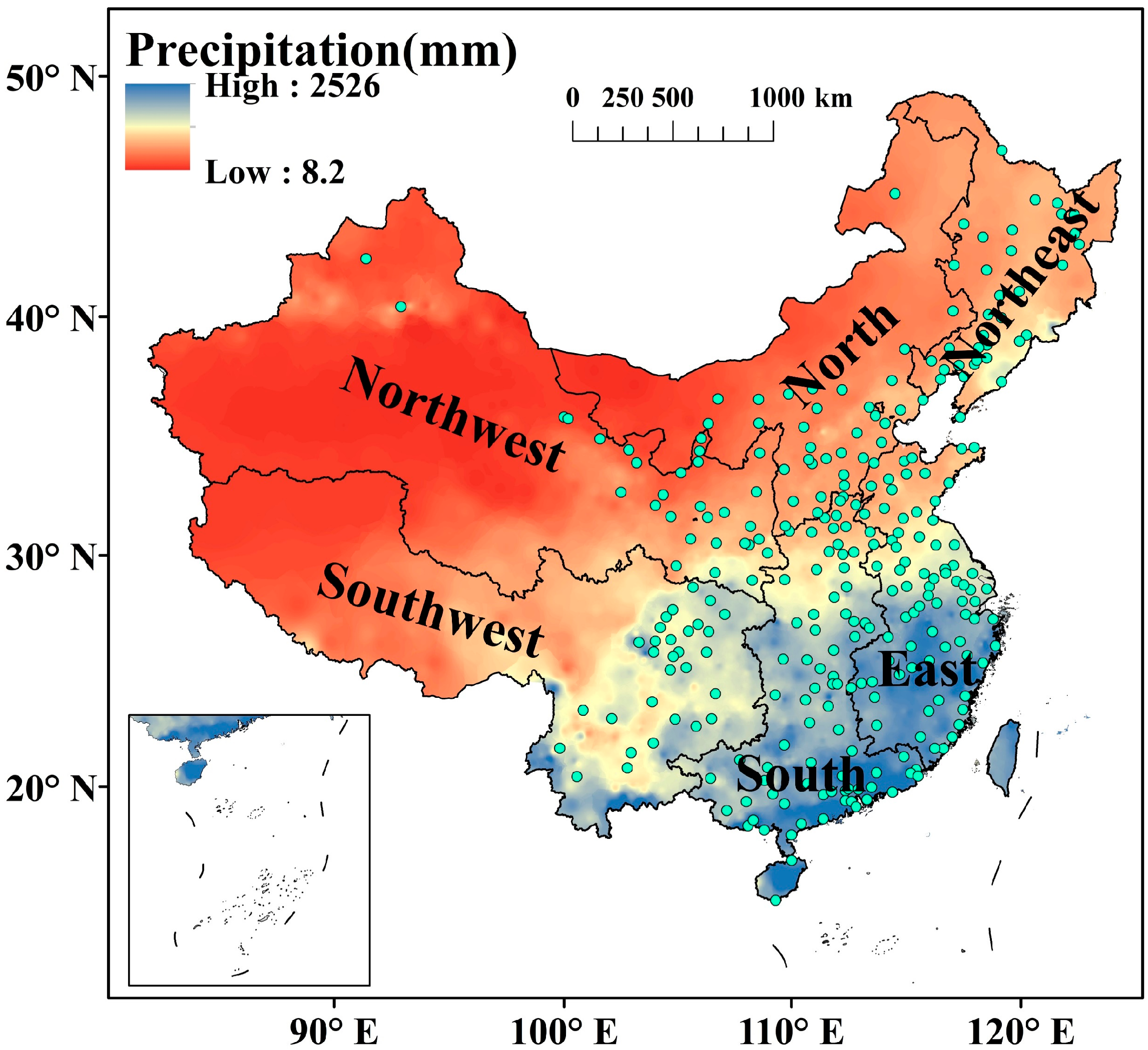
Figure 1. Geolocation of the selected 281 cities and six regions (Northwest, North, Northeast, East, South, and Southwest) of China in this study. The background information is annual precipitation across China.
Remotesensing 13 04428 g001
Figure 2. Spatial distributions of the variables used in the present study (using 2015 as an example). Note: SUHI = surface urban heat island intensity; ΔNDVI = urban−rural differences of NDVI; ΔPM2.5 = urban−rural differences of fine particulate matter; ΔPre = urban−rural differences of precipitation; NTL = urban nighttime light; Pop = the population at the end of the year.
Remotesensing 13 04428 g002
Figure 3. The overall framework of the study. Note: SUHI = surface urban heat island intensity; NDVI = normalized difference vegetation index; MODIS LST = Moderate Resolution Imaging Spectroradiometer land surface temperature; ESA CCI = European Space Agency’s Climate Change Initiative; SRTM DEM = Shuttle Radar Topography Mission Digital Elevation Model; MGWR = the population at the end of the year.
Remotesensing 13 04428 g003
Figure 4. Spatial distributions of MGWR’s local R2 in 2005, 2010, 2015, and 2018.
Remotesensing 13 04428 g004aRemotesensing 13 04428 g004b
Figure 5. Spatial distributions of the coefficients of ΔNDVI, ΔPrecipitation, and Intercept for the daytime MGWR model in 2005, 2010, 2015, and 2018.
Remotesensing 13 04428 g005aRemotesensing 13 04428 g005b
Figure 6. Spatial distributions of the coefficients of ΔNDVI, ΔPrecipitation, Intercept for the nighttime MGWR model in 2005, 2010, 2015, and 2018.
Remotesensing 13 04428 g006aRemotesensing 13 04428 g006b
Figure 7. Spatial distributions of the coefficients of NTL, ΔPM2.5, and Population for the daytime MGWR model in in 2005, 2010, 2015, and 2018.
Remotesensing 13 04428 g007aRemotesensing 13 04428 g007b
Figure 8. Spatial distributions of the coefficients of NTL, ΔPM2.5, and Population for the nighttime MGWR model in 2005, 2010, 2015, and 2018.
Remotesensing 13 04428 g008aRemotesensing 13 04428 g008b
Figure 9. Spatial distributions of the coefficients of ΔNDVI for the daytime MGWR model in the summer and winter of 2005, 2010, 2015, and 2018.
Remotesensing 13 04428 g009aRemotesensing 13 04428 g009b
Figure 10. Spatial distributions of the coefficients of ΔNDVI for the nighttime MGWR model in the summer and winter of 2005, 2010, 2015, and 2018.
Remotesensing 13 04428 g010aRemotesensing 13 04428 g010b
Table 1. Descriptive statistics for variables in this study.
VariableNumber of
Observations
MeanSTD1st Quartile2nd Quartile3rd QuartileReference
SUHI (°C)Daytime2810.8561.1250.4701.0331.465-
Nighttime2810.7030.5710.4390.7020.966
ΔNDVI (1/103)281−2.2181.171−3.027−2.377−1.502[58,59]
ΔPM2.5 (μg/m3)2810.3032.108−0.7570.2411.319[60,61]
ΔPre (mm)2814.93924.033−5.3155.21815.210[30,62]
NTL (DN value)28120.705.60717.50219.25521.968[28,63]
Pop (104 Person)2814.3283.0732.3823.6645.675[4,40]
Note: SUHI = surface urban heat island intensity; ΔNDVI = urban–rural differences of NDVI; ΔPM2.5 = urban–rural differences of fine particulate matter; ΔPre = urban–rural differences of precipitation; NTL = urban nighttime light; Pop = the population at the end of the year.
Table 2. Results of the ordinary least squares regression model applied to SUHI intensity and drivers in 2005, 2010, 2015, and 2018.
2005201020152018
DaytimeNighttimeDaytimeNighttimeDaytimeNighttimeDaytimeDaytime
ΔNDVI−0.735 ***0.208 ***−0726 ***0.337 ***−0.790 ***0.399 ***−0.776 ***0.386 ***
ΔPRE−0.013−0.0140.068 *0.0630.0370.100−0.0080.132 **
NTL0.082 **0.205 ***0.083 **0.056 **0.121 ***0.139 ***0.131 ***0.059
ΔPM2.50.000−0.012−0.036−0.0430.068−0.020.092 ***0.055
POP0.0030.0010.0190.0120.0340.060.040.074
R20.5450.0870.5400.1350.6660.1810.6580.176
Adj. R20.5370.0710.5320.1200.6600.1660.6520.161
AICC592.758788.989595.728773.649505.325758.541510.183757.353
RSS128.370257.435129.729243.80694.14823196.043231.459
Note: Coefficients provided in this table have all been standardized; ***, **, * refer to the respective significance at 1%, 5%, and 10% levels, respectively; AICc = corrected Akaike’s information criterion; RSS = residual sum of squares; Adj. R2 = adjusted coefficient of determination.
Table 3. Spatial autocorrelation statistics results for the SUHI intensity in each of the four time periods.
2005201020152018
DayNightDayNightDayNightDayNight
Moran’s Index0.4080.2610.4750.3340.5440.2460.5460.260
Z-score17.3111.0620.1916.0622.9310.40222.0810.538
p-value<0.001<0.001<0.001<0.001<0.001<0.001<0.001<0.001
Table 4. Diagnostics information for the classical GWR model in each of the three time periods.
2005201020152018
DaytimeNighttimeDaytimeDaytimeNighttimeNighttimeDaytimeNighttime
Bandwidth7388638674988378
R20.8040.5880.8510.8680.6320.6090.8610.619
Adj. R20.7560.5080.8100.8420.5450.5430.8320.535
AICC479.856662.772421.886342.88652.109634.155362.921655.341
RSS55.396116.22441.91936.968103.365110.24139.175107.310
Note: AICc = corrected Akaike’s information criterion; RSS = residual sum of squares; Adj. R2 = adjusted coefficient of determination.
Publisher’s Note: MDPI stays neutral with regard to jurisdictional claims in published maps and institutional affiliations.