Abstract
Remote sensing applications of change detection are increasingly in demand for many areas of land use and urbanization, and disaster risk reduction. The Sendai Framework for Disaster Risk Reduction and the New Urban Agenda by the United Nations call for risk monitoring. This study maps and assesses the urban area changes of 23 Mexican-USA border cities with a remote sensing-based approach. A literature study on existing studies on hazard mapping and social vulnerability in those cities reveals a need for further studies on urban growth. Using a multi-modal combination of aerial, declassified (CORONA, GAMBIT, HEXAGON programs), and recent (Sentinel-2) satellite imagery, this study expands existing land cover change assessments by capturing urban growth back to the 1940s. A Geographic Information System and census data assessment results reveal that massive urban growth has occurred on both sides of the national border. On the Mexican side, population and area growth exceeds the US cities in many cases. In addition, flood hazard exposure has grown along with growing city sizes, despite structural river training. These findings indicate a need for more risk monitoring that includes remote sensing data. It has socio-economic implications, too, as the social vulnerability on Mexican and US sides differ. This study calls for the maintenance and expansion of open data repositories to enable such transboundary risk comparisons. Common vulnerability variable sets could be helpful to enable better comparisons as well as comparable flood zonation mapping techniques. To enable risk monitoring, basic data such as urban boundaries should be mapped per decade and provided on open data platforms in GIS formats and not just in map viewers.
1. Introduction
At the international level, the call for monitoring urban growth and monitoring disaster risk led to a series of strategies in urban development and disaster risk reduction [1,2]. Findings have shown that urban areas often grow into areas of increased disaster risk, such as coastal or fluvial hazard zones [3]. Global attention to a related topic of population dynamics, the migration topic [4], has lately been expanded on so-called environmental drivers of migration [5]. Cross-border assessments are in demand, too, since natural hazards such as floods do not stop at administrative boundaries [6,7]. However, human planning and activity influence risk exposure, vulnerability, and resilience differently within different administrative boundaries [8]. These differences often become most apparent along national borders, for example, by the different extents of urban development. However, what is missing so far are cross-border urban change assessments that combine urban growth and natural hazard aspects. These assessments are important since hazards such as floods, earthquakes or storms do not stop at administrative borders. However, exposure, vulnerability and preparedness vary at national borders on each side, resulting in different risk patterns. Understanding natural hazard and risk patterns cannot only help to save human lives but also can contribute to solving conflicts. For example, migration is an additional factor to consider at national borders. In 2021, between 14–16,000 immigrants from Haiti and other countries had to camp under a bridge at a Mexican-USA border city, Del Rio, a major transportation and trade hub [9,10,11]. If a flood or tornado had occurred during this time, that binational event would have become an additional human crisis. Another constraint often is data availability to warn people of hazards on both sides of a national border or to include such knowledge into spatial planning. Therefore, it is important to utilize spatial assessment capabilities to inform the public and decision-makers about the risk of natural hazards and how this risk varies across borders and develops over time.
The Mexican-US border receives media attention due to the influx of migrants and associated problems with it. While this cross-border region experiences urban growth, the exposure to natural hazards such as riverine floods also may grow. All major cities covered here are along rivers. Social vulnerability is at the highest levels in these border areas on the US side [12], while on the Mexican side it is low to medium [13]. At segments, the Mexican-US border is a limitrophe, where the river defines the international boundary. River courses are subject to change due to flooding, due to natural or man-made reasons [14], which is another reason flood monitoring along international borders is of high national interest. Illegal border crossing and tunneling activities have modified drainage patterns during monsoonal floods [15]. Floods do not stop at borders or even flood the areas directly along a border wall, for example, in Nogales [16]. This has led to cross-border cooperation between scientists developing joint assessments and cooperation between administrations to build joint flood defenses.
Urban growth studies using remote sensing data have become a standard approach [17,18,19]. However, combining it with growth into natural hazard-prone areas is less common. There is an increasing interest in multi-hazard and multi-risk assessments, utilizing demographic data in spatial assessments for aspects of resilience [20] or vulnerability [21]. However, aspects of urban growth that are linked to risks and vulnerabilities, such as slum areas and poorer populations, are already analysed using remote sensing at different time intervals [22]. Another gap is the utilization of declassified satellite data for change detection. There are few studies yet using such data for change detection of coastlines [23], glacier changes [24,25], forest cover change [26], land-use change in general [27], or urban growth [18,28,29,30]. Some recent developments have analyzed constraints of image interpretation by humans [29,30] and opportunities by multitemporal and multi-criteria assessments of urban change and urban risks [31,32].
This article aims at analyzing urban growth and its dynamics along cross-border cities as a starting point to understand and document natural hazard exposure growth. International programs such as the Sendai Framework [2] and its related monitoring [33] encourage disaster risk monitoring using spatial assessment. This assessment and information may, later on, be expanded to analyze different social vulnerability and resilience profiles and include other natural and man-made hazards, too. Remote sensing-related international bodies such as UNSPIDER underline the demands and opportunities remote sensing data provide for a more comprehensive risk monitoring.
Urban growth assessments using remote sensing data are widely applied for individual Mexican cities [34] or US counties [35]. However, what is novel in this article is the assessment of all major cities along the border in one assessment. Moreover, the typical time span covered by most studies ranges back to the earliest Landsat data, which is expanded by this study on the range back to the 1940s using aerial imagery, and CORONA satellite imagery starting from the 1970s, where available. In addition, the assessment also investigates how urban growth varies between the Mexican and US sides of the border and how this growth expands into flood hazard exposed areas differently.
The main research question guiding this article is: How did Mexican-US border cities develop over time and concerning flood hazards?
2. State of the Art
2.1. Using Documented Search Terms
Systematic assessment of the existing literature identifies studies on this thematic area. The focus follows the main research question above, identifying Mexican and US cities and related studies on urban growth, usage of remote sensing in those studies, and relations to disaster risk. Many synonyms were considered and documented in the literature search, such as urban growth or sprawl or expansion (Table A1). Another term with many variations identified in this local context is ‘twin cities’ of the border [36] or ‘sister cities’, ‘cross-border towns’, ‘transboundary’ urban areas, etc., along the Mexican-US border, have long been a topic of investigation [37], using remote sensing data supported such assessments, especially after Landsat satellite imagery became publicly available.
2.2. Urban Growth Analysis along the Mexican-US Border
Research on border cities or urban areas at the northern border of Mexico concentrates on the amount of urban growth (see Table 1) and disparities of socio-economic conditions [38,39,40] or related marginality in terms of access to basic services [41]. Studies on individual (twin) cities go more in-depth on topographic, demographic, and infrastructure factors contributing to or showcasing growth [42,43].
2.3. Usage of Aerial and Satellite Imagery for Measuring Urban Growth Related to Hazards
Aerial imagery has been used to capture land cover change, for individual local areas such as Tijuana, with data ranging back to 1938 [44]. Satellite imagery is frequently used to analyze and document urban growth or model future urban growth [45,46]. For individual cities or transboundary cities along the area of interest, urban growth analyses using remote sensing include studies on Tijuana [47], Ciudad Juarez and El Paso [48], Mexicali [49], Agua Prieta, and Douglas [50]. No individual study on urban growth, sprawl, or expansion could be found for a few cities using remote sensing, including San Diego, Calexico, Ciudad Acuna, Del Rio, Piedras Negras, and Eagle Pass, San Luis Rio Colorado, or San Luis. No single study could be found for a few cities, either as individual study or in conjunction with other cities, for example, Ciudad Acuna, Del Rio, San Luis Rio Colorado, San Luis, Reynosa, Hidalgo, or Matamoros. These remote sensing studies probably exist but have not been identified using several search terms (see Table A1). Few studies have analyzed several cross-border cities along this border regarding urban growth, and if so, not always their twin cities and not all major cities together [51]. Few other studies investigated several cities along the border but only in one country [52,53].
2.4. Flood Hazard and Risk Research
Water availability is a topic in this area due to water scarcity in arid regions and occasional floods. Land-use change and urban growth often exacerbate water scarcity, different on each side of the border, depending on different growth rates [54]. A watershed analysis is conducted as a basis for identifying flood zones in Nogales [16]. Research on climate change adaptation covers the interrelation between urbanization and water scarcity [55] and related flood or landslide hazards [47]. Social vulnerability in conjunction with flood hazard has been analyzed using census data for Ciudad Acuna and Del Rio [56].
2.5. State-of-the-Art Classification Models
Spatial mapping of urban features and growth using remote sensing images has a long tradition of classification methods [57,58]. Recently, many machine or deep learning forms have been applied [59,60,61], using neural networks for quite some time already [62,63]. Support vector machine or random forest are common approaches [64,65]. Developments in the past years include multi-temporal, multi-spectral, and multi-modal analyses in different areas of application concerning land use [60,66,67,68,69]. Time series analysis is a field especially useful for urban growth detection [70,71], even despite cloud coverage [72]. Image fusion to enhance spatial resolution is also an established field and has been long applied with Landsat images and other multi-spectral data [73,74,75], but has lately been advanced by modern approaches with hyperspectral data [76]. Object-based classification often targets building extraction and contributes to urban object-based image analysis [77,78]. Another emerging field is radar satellite data applied for urban studies [79]. LiDAR data is also increasingly used for both urban and natural hazard assessments [80,81]. Night-time light or emission is another idea capturing urban features with remote sensing [82,83] and dates back to early applications of thermal information, too [84]. NDVI is also used for urban vegetation, but can also be used for other urban feature identification [58,82].
2.6. Summary of Major Gaps Identified
Table 1 shows several studies on individual cities along the Mexican-US border concerning urban growth, of whom many are using remote sensing. There are fewer studies on multiple cities at once, and by our search terms (see Table A1), no comprehensive study covering all cities was identified. Individual city analyses often are covered by the same or similar author teams for successive studies. The covered data range varies much, complicating direct comparisons and underlines the need for a study that uses a uniform approach. Of course, this is dependent on data availability. The data time ranges go back to the 1970s and are mostly conducted using early Landsat data. Even earlier CORONA satellite data or aerial imagery are missing. Few findings combine urban growth with flood hazard assessment, and even fewer cover social vulnerability.

Table 1.
Literature for individual cities of the Mexican-US border covering urban growth with mapping, and other analysis.
Table 1.
Literature for individual cities of the Mexican-US border covering urban growth with mapping, and other analysis.
| Authors | Abstract or Full-Text | Cities | Remote Sensing (and Data Range) | Hazard | Social Vulnerability |
|---|---|---|---|---|---|
| Korbulic 2012 | Full-text | Tijuana & San Diego; Mexicali & Calexico; San Luis RC & San Luis; El Centro; Yuma | Yes, 1985–2010 | No | No |
| Sánchez Rodríguez & Morales Santos, 2018 | Full-text | Tijuana | Yes, 1972–2014 | Climate Change, flood, landslides | Yes |
| Leyva–Camacho et al., 2010 | Full-text | Mexicali | Yes, 1990–2005 | No | No |
| Norman et al., 2004 | Full-text | Agua Prieta & Douglas | Yes, 1973–2000 | No | No |
| Myint et al., 2014 | Abstract | Nogales & Nogales | Yes, 1984–2004 | - | - |
| Norman et al., 2009 | Full-text | Nogales & Nogales | Yes, 1975–2002 | No | No |
| Norman et al., 2010 | Full-text | Nogales & Nogales | Yes | Flood | No |
| Mubako et al., 2018 | Full-text | Ciudad Juarez & El Paso, Las Cruzes | Yes, 1990–2015 | No | No |
| Zhao et al., 2017 | Abstract | Nuevo Laredo & Laredo | Yes | - | - |
| Zhao et al., 2020 | Full-text | Nuevo Laredo & Laredo | Yes, 1985–2014 | No | No |
| Pena 2012 | Full-text | Rio Grande City-Roma, McAllen-Edinburg-Mission, Harlingen-Brownsville | Yes, 1990–2010 | No | No |
| Leigh et al., 2009 | Full-text | Counties Cameron, El Paso, Hidalgo, Maverick, Willacy | Yes, 1996–2006 | No | No |
3. Method
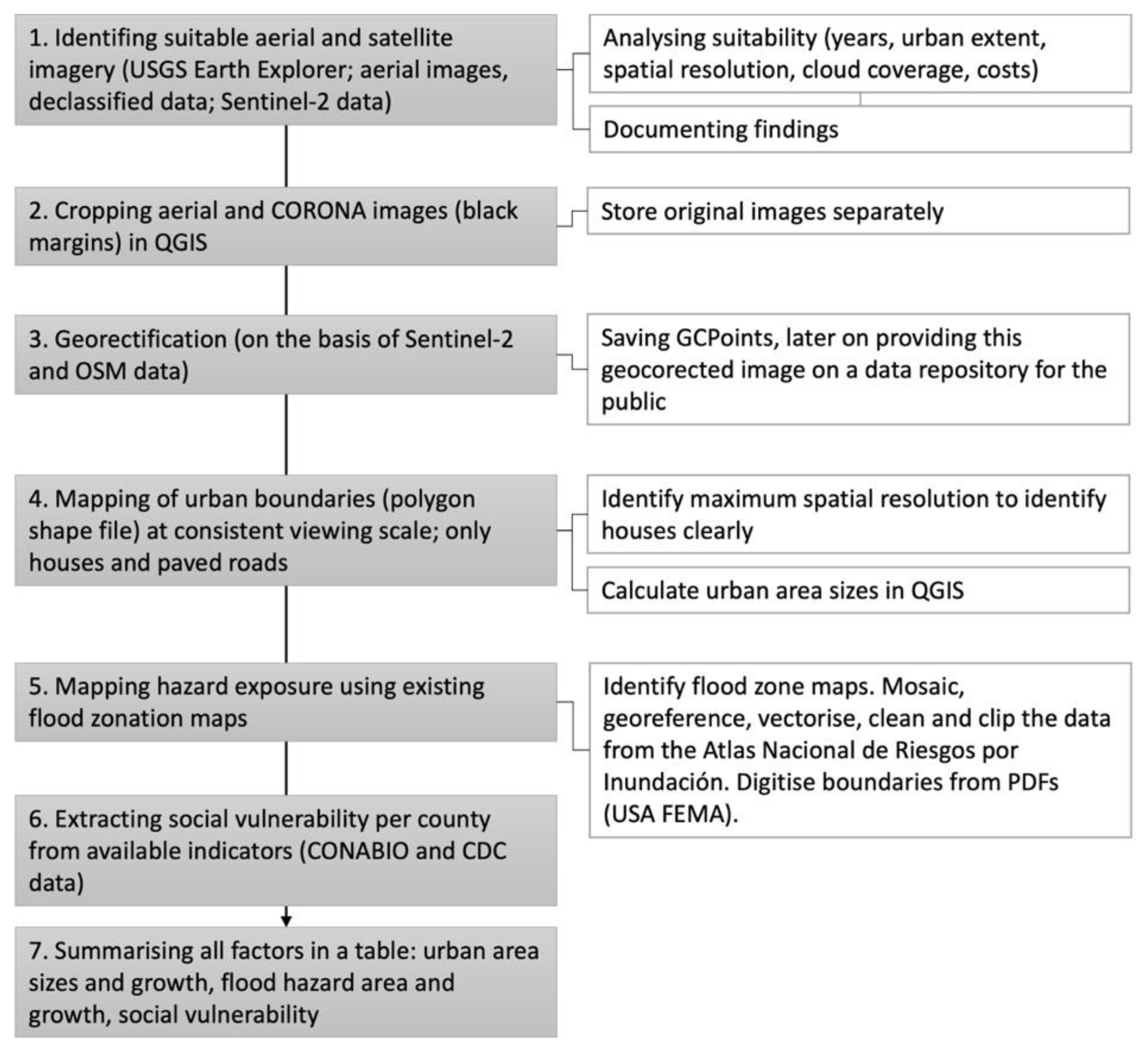
A spatial assessment using a Geographic Information System (GIS) combines aerial and satellite imagery, open-source maps, and demographic information. The approach is a spatial risk assessment that analyzes hazard and impact features: spatial signatures and growth of settlements, hazard zones, and information about social vulnerabilities. The stepwise assessment approach first identifies suitable remote sensing data from multiple temporal phases of urban development, then conducts cropping and georectification to enable further analysis in a GIS (Figure 1). Next, urban boundaries are mapped, and flood exposure and social vulnerability are extracted from official sources. Finally, all information is integrated into a table that compares important spatial risk features: of urban exposure, flood zones, and their respective growth rates, and spatial differences in social vulnerability.

Figure 1.
Flowchart of methodological steps in this article.
3.1. Data Used
Literature sources have been searched on google scholar using specific key search terms documented in the table in Table A1. Census statistics were obtained from public websites, which appeared to be official governmental and, therefore, relatively reliable statistics (see the table in Table A2).
Spatial data on urban extent were analyzed from satellite, and aerial images (see Table 2 and Table A2) since existing urban footprint data or urban boundaries were not found to reach back into the past far enough to capture the massive growth that occurred. The USGS Earth Explorer data portal was used since it is one of the most comprehensive data archives, a reliable source for decades, and provides rare data reaching back into the past. Aerial images have been accessed to the earliest date accessible, and 23 image tiles have been manually selected, downloaded, and georectified. In areas where those imageries were not available, additional old satellite imagery has been obtained from this platform; 9 images of CORONA satellite data have been manually selected, downloaded, and georectified. Images of Sentinel 2 satellite data have been used via a WMS service in QGIS to capture the most recent urban perimeters.

Table 2.
Aerial and satellite imagery used for this study.
The aerial imagery we used has a scale of 1:12,000–1:60,000, with one exception (1:130,000). However, in most places, only one set of data was available. Only for selected locations such as El Paso, aerial imagery in different scales was available; the oldest data from 1:3120 (1950) to 1:50,000 (1942). Since the images from 1942 were of relatively bad quality, we used aerial images from 1956 for these two border cities (Ciudad Juarez and El Paso) and as a compromise between good quality, resolution, and frame size to make the manual download, georectification, and digitization work feasible within a reasonable time.
3.2. Methodological Steps
The case study areas are selected according to urban settlements on both sides of the Mexican-US border, which also have an assumed natural hazard exposure due to rivers nearby. Due to the number of possible locations, only major twin cities are selected, with at least around 100,000 inhabitants combined. Tecate, MX is excluded for this reason, for example.
Using less known older aerial and satellite imagery (declassified data from CORONA, GAMBIT, HEXAGON programs), the pre-existing land surface from the 1940/1950s and 1970s is mapped and compared with areas recently overgrown by settlement and infrastructure (using Sentinel 2 data). This is conducted in QGIS, an open-source software, so that the results can later be shared with the public. QGIS also allows computing on different computers (Microsoft, Apple, Linux). From aerial images, the black frames were cut to enable mosaics better. The images were georectified, ground control points saved, to later on sharing this processed data publicly. The aerial images, in scales between 1:20,000 and 1:130,000) were manually georectified to WGS84 UTM zone 14N and EPSG 32614 in QGIS at scales below 1:2500 using Sentinel 2 satellite data. Ground control points are documented, and polynomial transformations 1–3 were compared to identify the best fit (Table with details provided in our open data repository). Since arid lands and semi-desert areas are involved, georectification in these areas was rather difficult. The amount of GCP was therefore focused and maximized within urban areas.
A maximum spatial resolution of different scales and products was identified (see data sub-sections below) and then consistently used for georectification and digitization of urban built-up areas. Visual and manual mapping was conducted since the grayscale images’ spatial resolution is often not sufficient for supervised or object-based classification. Polygon shapefiles are created to enable area calculation later on. The urban area coverage from the aerial images was mapped at a scale of 1:2000 to 1:5000. Suburban areas or single houses at the city perimeter were excluded when the distances between the perimeter and the adjacent urban area signature exceeded 100 m.
The recent urban land use coverage from the year 2020 was mapped using Sentinel 2 data. At a scale between 1:10,000 to 1:25,000, urban boundaries were mapped according to the visibility of buildings, airports and runways, and industrial sites. Road and rail infrastructure were only taken into account within the city boundaries. Urban parks were included when they were surrounded by the urban features described before. Golf courses were excluded as well as city areas with roads only such as new designated urban areas. Urban features of suburban development were excluded when the distance to the core city area exceeded 1 km. The guiding idea was to cover urban areas that could potentially receive flood damage. River embankments were excluded from mapping when not covered by the built environment to enable mapping of flood risk more precisely. Each city received one separate shape boundary. Since we were mapping 23 cities, the time factor played an important role, and manually creating the boundaries was more time-efficient than the classification methods we tried.
The mapping of urban areas via aerial and satellite images using GIS also permits calculating the growth of urban areas. This enables a comparison of relative growth but is not understood to be exact. Limitations of aerial size calculations can be due to several reasons such as missed built-up areas due to image quality, the skill of the visual interpretation, or re-projection [85]. Exceptional growth rates such as for San Luis are due to the tiny area in the 1950s and the spatial resolution of the images and therefore are not to be understood as absolute, only relative indications of growth rates.
Flood exposure analysis is conducted using publicly available data as a GIS file for download (see data sections and Table A2). The flood area polygons are clipped with the mapped urban areas for each time period. Area sizes are calculated in the GIS. Data for flood zones in Mexico were identified in the Atlas Nacional de Riesgos por Inundación (ANRI, see Table A2) but were unavailable as shapefiles. An email was sent to CENAPRED to request the data, but no reply was received. Therefore, the respective best available flood scenarios (100 years, except for Ciudad Juarez, where 50 years and 100 years were combined) were mapped for each city using screenshots of the Atlas. Two different scenario types are available, with better modeling resolutions for selected cities. These were mosaiced, georeferenced, vectorized, cleaned, and then clipped with the urban areas in QGIS.
Social vulnerability data were retrieved from public platforms of official institutions, too.
Data processed and generated were provided to the public on a data repository: (https://riskncrisis.wordpress.com/data accessed on 31 October 2021). At the end of all methodological steps, the factors contributing to urban area, growth, hazard, and vulnerability were summarized in a table that allows for comparison.
4. Results
The results of the mapping and literature search were documented in the maps and tables below.
4.1. Urban Area Size and Growth
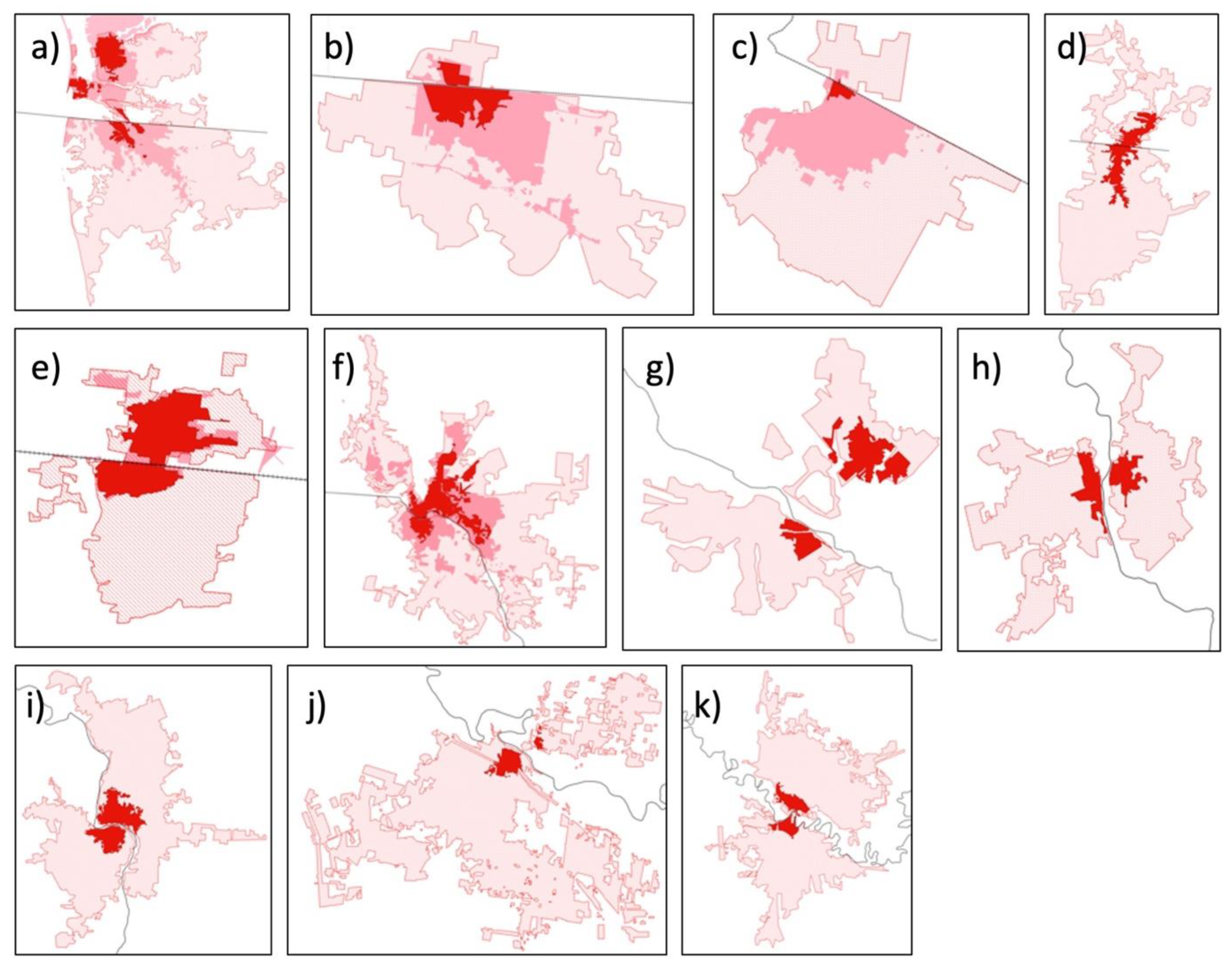
The cities were presented from west to east, starting with Tijuana and San Diego in the west, and ending with Matamoros and Brownsville in the east (Figure 2). The contrast of urban development at the national border is visible in the urban shapes that were mapped. The border makes an artificial divide limiting urban connectivity but also urban expansion, which is especially the case for Tijuana/San Diego, Mexicali/Calexico, or San Luis R.C./San Luis. All cities presented here are located directly at or close to a river. In several cases, the river provides the natural border, which is visible by the border signature in the maps.
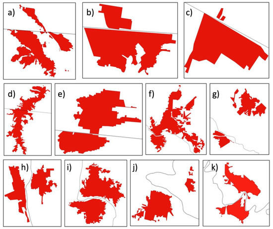
Figure 2.
Urban areas in the 1940s–1950s extracted from aerial images; (a) San Ysidro and Tijuana 1955, (b) Mexicali and Calexico 1953, (c) San Luis Rio C./San Luis 1949, (d) Nogales 195; (e) Agua Prieta and Douglas 1958, (f) Ciudad Juárez and El Paso 1956, (g) Ciudad Acuna and Del Rio 1950, (h) Piedras Negras and Eagle Pass 1947; (i) Nuevo L. and Laredo 19, (j) Reynosa and Hidalgo 1946, (k) Matamoros and Brownsville 1946.
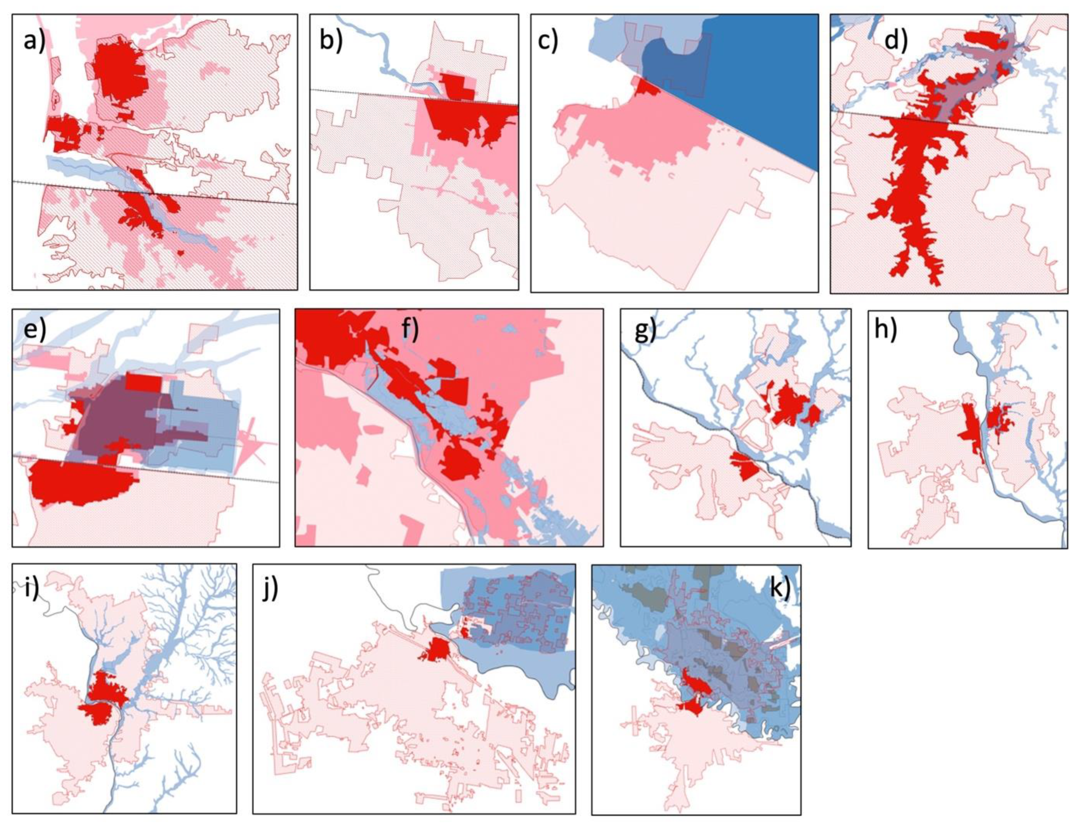
As visible from the aerial mappings (Figure 2), the urban areas in the past were smaller on the Mexican side compared to the USA side of the border for Agua Prieta, Ciudad Juárez, and Ciudad Acuna. On the US side, the cities of San Ysidro and Imperial Beach city (San Diego area), Calexico, San Luis (Yuma is close by), and Hidalgo (McAllen is close by) were smaller than their Mexican counterparts. This pattern has remained consistent during massive urban growth in the 1970s and up to the 2020s, only for Ciudad Acuna (Figure 3). Agua Prieta and Ciudad Juárez have grown in size more than their US counterparts. San Ysidro is now part of the San Diego metropolitan area, which is difficult to delimit to the north. Calexico, San Luis, and Hidalgo on the US side have remained smaller than their Mexican counterparts. However, their hinterland cities, Yuma and McAllen, have grown massively, which is not shown here since they are not the direct border counterparts.
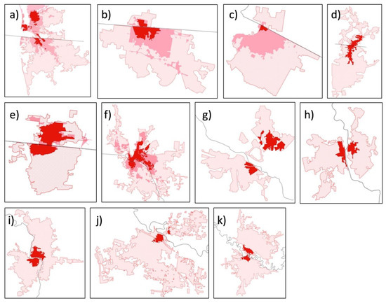
Figure 3.
Urban areas and urban growth from the 1940s to 2020 extracted from aerial images, CORONA, and Sentinel 2 satellite images; (a) San Diego area and Tijuana 1955, 1972, 2020, (b) Mexicali and Calexico 1953, 1976, 2020, (c) San Luis Rio C./San Luis 1949, 1972, 2020, (d) Nogales 1951, 1976, 2020, (e) Agua Prieta and Douglas 1958, 1976, 2020 (f) Ciudad Juarez and El Paso 1956, 2020, (g) Ciudad Acuna and Del Rio 1950, 1978, 2020 (h) Piedras Negras and Eagle Pass 1947, 2020, (i) Nuevo L. and Laredo 1947, (j) Reynosa and Hidalgo 1946, (k) Matamoros and Brownsville 1946.
As taken from census data (Table 3), urban growth rates indicate relatively higher growth rates of almost all Mexican cities compared to their US neighbor cities, except for Brownsville. Tijuana, San Luis Rio Colorado, and Ciudad Juárez had the highest growth rates. This may indicate the importance of investigating a higher percentage of growth into potential hazard zones as well.

Table 3.
Analyzing urban growth of the cities along the Mexican-US border, based on census data (data sources: microregiones.gob.mx; inegi.org.mx; census.gov; texasalmanac.com, all accessed on 30 September 2021).
Data limitations occur for data from the past for some cities or counties. Therefore, the cities of Hidalgo and McAllen have to be presented by merged population numbers. Data from the 1950s was not available for San Luis in the USA, and therefore, the already very low population data from 1970 were used. San Luis was built as a border post in the 1930s. For Imperial Beach city, data from 1960 were available and not from 1950, which may infer an error that may underestimate the growth rate a bit.
4.2. Analysing Urban Area Sizes from Remote Sensing Data
The urban areas were calculated from the aerial and satellite images (Table 4). Urban growth has happened in all cities but varies in area and population growth factors.

Table 4.
Area sizes and growth as calculated from the aerial and satellite images.
4.3. Flood Hazard Exposure Mapping
While potential exposure areas in total have grown in all cities, even their relative share of the urban area has increased in 5 US and 4 Mexican cities (last two columns in Table 5 and Table 6).

Table 5.
Development of hazard exposure as calculated by the flood zones from the Atlas Nacional de Riesgos por Inundación overlapping with the urban areas mapped on the Mexican side.

Table 6.
Development of hazard exposure as calculated by the flood zones from FEMA overlapping with the urban areas mapped.
For the USA, hazard exposure was analysed using FEMA flood zone data (dates vary between 1980–2020), conducting a GIS analysis of urban areas overlapping with the flood zones (Table 6).
Flood hazard zones were obtained for the US cities from FEMA online (see Table A2) and downloaded as shapefiles. Only for Hidalgo and Laredo, were the maps available as printed versions only, and thus we digitized the flood areas. For the other cities, from the shapefile S_FLD_HAZ_AR, the potential flood zones were extracted by selecting the tiles marked with FLD_ZONE AE, AH, AO, AR, A99, manually from the map for the respective river sections, and tiles marked with 2 PCT Flood Chance (Zone X, extreme flood), separately (Figure 4). However, a visual check with the print version of the FEMA maps was necessary to adjust to the local context, where not always all those categories made sense to include.
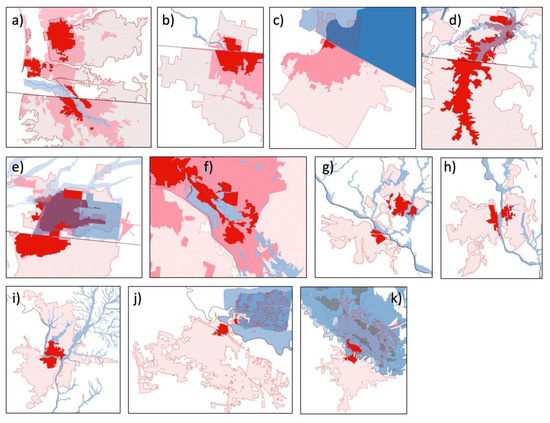
Figure 4.
Flood zones (FEMA) on the US side; (a) San Diego area: Tijuana river, (b) Calexico: Rio Nuevo, (c) San Luis: Rio Colorado, (d) Nogales: Arroyo, (e) Douglas: Whitewater Draw, (f) El Paso: Rio Grande, (g) Del Rio: Rio Grande, (h) Eagle Pass: Rio Grande, (i) Laredo: Rio Grande, (j) Hidalgo: Rio Grande, (k) Brownsville: Rio Grande (data sources: Table A2).
Hazard exposure cannot be directly compared between both countries because of different modeling and mapping approaches (see discussion). In addition, hazard exposure cannot be directly compared between the 1940s and today due to major river training measures conducted, such as along the Tijuana River or the Rio Grande River in Reynosa. That means that for the San Diego area, our flood area exposure estimation for the 1950s might be inaccurate in terms of absolute area. In addition, in some areas such as in San Luis, we assumed overtopping or breach of existing flood protection measures, which would need further analysis in more detail. However, the overall assessment looks at cross-regional and relative risk growth, where such error margins still do not change the overall picture.
4.4. Comparing Existing Social Vulnerability Data
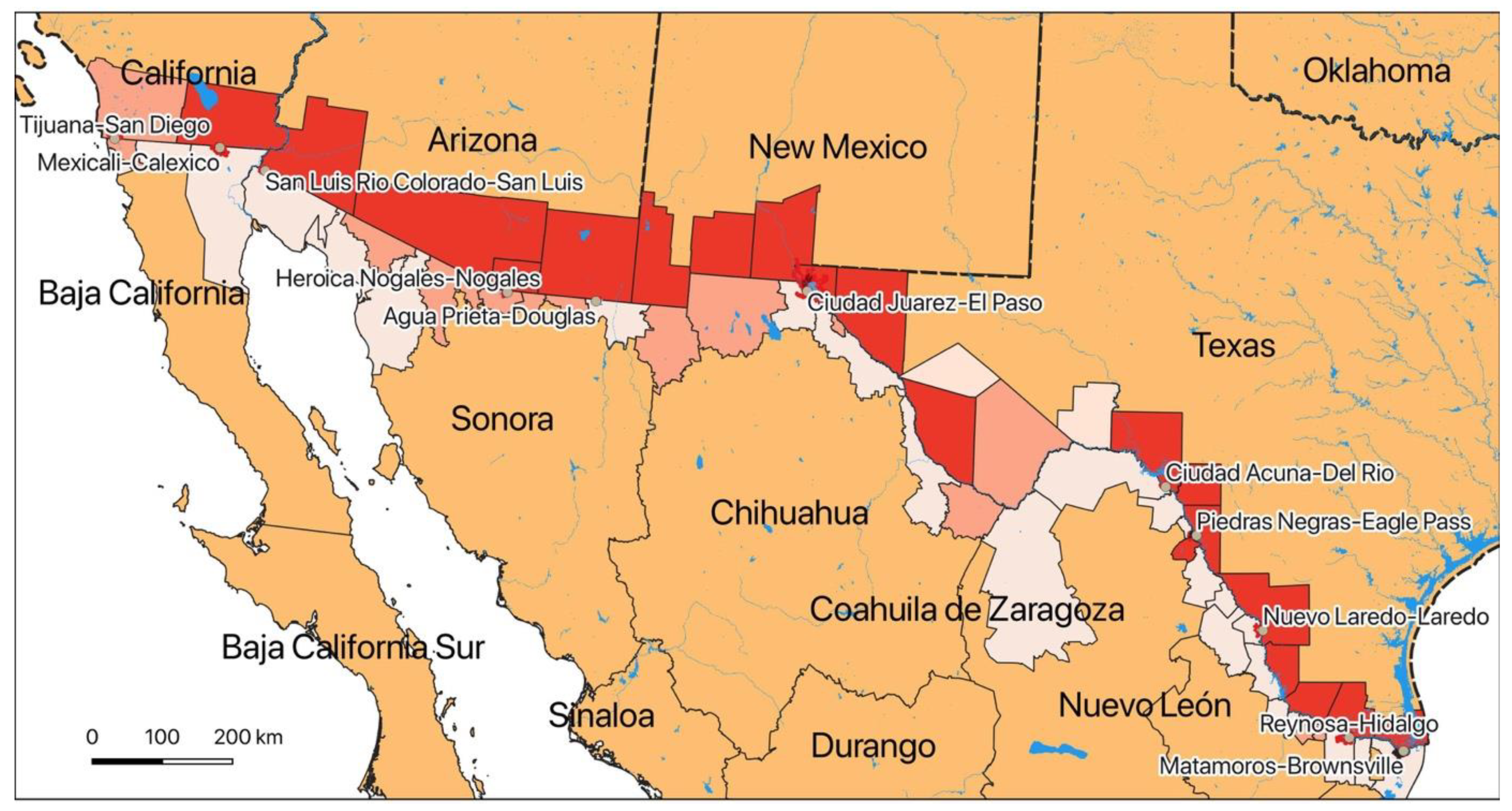
The SVI of the US CDC reveals that almost all southern US states exhibit a relatively high social vulnerability (CDC 2021: Table A2). Along the US-Mexican border, almost all counties are within the highest social vulnerability scores for the year 2000, except San Diego County, which is moderate to high, and Jeff Davis County (TX), which is low to moderate. Comparing the SVI at its earliest availability (2000) with its most recent (2018) reveals few changes in this pattern. The SVI index shows changes to lower levels of vulnerability for Brewster and Terrel counties, both located in Texas. The CDC SVI themes reveal that all counties exhibit high minority and language-related vulnerabilities. Social vulnerability differs for housing and transportation, which may indicate interesting areas for further analysis. The SVI for the Mexican side reveals a different picture. Vulnerability is quite heterogeneous along the Mexican-US border; medium and low to medium social vulnerability levels prevailed in 2010. Medium vulnerability is most prevalent along the Arizona and New Mexico border. While in the USA, vulnerability levels have decreased in two counties, in Mexico, SVI has been low to medium in 2000 for all counties, except for Janos county in Chihuahua. The map shows the SVI for 2010 on both sides of the border (Figure 5). This is the latest year for which both countries have produced the index. More recent indices are published as resilience indices in Mexico and can therefore not directly be compared. Different compositions of variables selected further constrain direct comparison of the Mexican and US SVI, and while the Mexican SVI is represented in 5 classes, the US index is presented in 4 classes. Even the original variables differ, and requests for obtaining original data were not answered. The latest SVI data at higher spatial resolution was obtained for the USA using CDC census tract data from 2018 (see Table 7 for results, Table A2 for data sources).
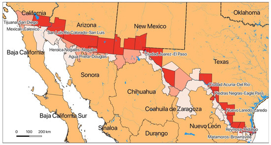
Figure 5.
SVI 2010 for municipios in Mexico (CONABIO) and counties in the USA (CDC) along the shared border of both countries. Darker colors (red) represent higher vulnerability (data sources: Table A2).
More detailed and context-specific SVI or social vulnerability analyses would be of interest for the specific cities themselves. However, such analyses are somewhat fragmented and available by individual studies of researchers for a few of those cities yet. Another constraint comparing the Mexican and US SVI is a composition of variables, the aggregation method, and other aspects of SVI indicator methodology [86,87]. Therefore, a comparison of both sides of the border would warrant more research and is limited here.
An additional aspect adding to social vulnerability is the high mobility and migration at the border. Statistics show that around half a million encounters have been registered on the US side, (as of March 2021, per one fiscal year) with half of the migrating people crossing the Mexican-US border from Mexico (CBP 2021, see Table A2). Ratios were highest for the Rio Grande Valley region, followed by Tucson, El Paso, Del Rio, San Diego, and Laredo. They were lower for El Centro, Yuma, and Big Bend. Of the 159,470 persons registered at the Rio Grande Valley, 20,964 were single minors, indicating a population group with a specific social vulnerability. However, these numbers do not show the number of persons illegally crossing the border, which must be added to the numbers of populations potentially exposed to natural hazards such as riverine, pluvial flood, or storms.
4.5. Summary of Urban and Flood Exposure Growth Factors Contributing to Overall Disaster Risk
The spatial and statistical analysis provides some indications for disaster risk and for capturing its dynamics. Table 7 lists some main results from the previous analysis steps. In selecting the top 3 cities for Mexico and the US, those with the highest population sizes in 2010 also have the highest urban areas in 2020. However, these cities do not necessarily exhibit the highest relative social vulnerability or flood exposure. On the Mexican side, Tijuana is not only is the biggest city with the high area and population growth rates, but it also lies in an administrative area (Mexican: municipio) with a social vulnerability that had increased between 2000 to 2010. This puts Tijuana highest in the categories related to existing static flood risk and highest in the dynamic development of disaster risk. Of course, these few categories only indicate disaster risk, out of many more aspects that would have to be considered for a holistic risk assessment. Ciudad Juarez also exhibits high growth rates, as well as San Luis Rio Colorado and Ciudad Acuna on the Mexican side. On the US side, the San Diego area, El Paso, and Laredo are the biggest agglomerations, whereas the growth dynamic is higher in San Luis, Nogales, and McAllen/Hidalgo. Social vulnerability varies across county/municipio levels. The highest rates at the city level in the USA are in Nogales, Calexico, and Eagle Pass. Census tracts reveal wider disparities, with the lowest rates in Imperial Beach and highest rates in El Paso (Table A3). Flood exposure by area size is highest for 2020 for Tijuana, Matamoros, Ciudad Juarez, Brownsville, Hidalgo, and Laredo. Flood exposed area has grown fastest in San Luis on both sides of the border, Hidalgo, but is also significant for Reynosa, Matamoros, and Brownsville.

Table 7.
Summary of urban growth and risk factors analyzed in this study.
Table 7.
Summary of urban growth and risk factors analyzed in this study.
| City in Mexico | Population 2010 | City Area 2020 (km2) | Area Growth Factor | Population Growth Factor | SVI 2010 (Municipio/County) | SVI 2018 Census Tract (Mean Value) | Flood Exposure 2020 (km2) | Flood Exposure Growth Factor 1940–2020 |
|---|---|---|---|---|---|---|---|---|
| Tijuana | 1559,683 | 388 | 46 | 24 | medium | - | 87 | 23 |
| Mexicali | 936,826 | 194 | 18 | 8 | low | - | 50 | 17 |
| San Luis Rio Colorado | 178,380 | 65 | >100 | 13 | low | - | 16 | >100 |
| Nogales | 220,292 | 44 | 14 | 8 | medium | - | 7 | 6 |
| Agua Prieta | 79,138 | 26 | 9 | 6 | low | - | 5 | 4 |
| Ciudad Juarez | 1332,131 | 313 | 23 | 10 | low | - | 62 | 15 |
| Ciudad Acuna | 134233 | 37 | 16 | 10 | low | - | 15 | 10 |
| Piedras Negras | 150178 | 45 | 1 | 5 | low | - | 7 | 10 |
| Nuevo Laredo | 384,033 | 96 | 1 | 6 | low | - | 35 | 13 |
| Reynosa | 589,466 | 120 | 1 | 8 | low | - | 51 | 53 |
| Matamoros, Mexico | 449,815 | 109 | 0 | 4 | low | - | 76 | 34 |
| City in USA | ||||||||
| San Ysidro | 28,008 | 8 | 7 | 3 | high | 0.803 | 2 | 0 |
| Imperial Beach city | 51,332 | 49 | 8 | 3 | high | 0.650 | 1 | 0 |
| Calexico | 38,573 | 16 | 7 | 6 | highest | 0.923 | 0 | 0 |
| San Luis | 27,909 | 9 | >100 | >100 | highest | 0.837 | 9 | >100 |
| Nogales | 20,839 | 18 | 8 | 8 | highest | 0.927 | 5 | 5 |
| Douglas | 17,509 | 13 | 2 | 2 | highest | 0.902 | 9 | 2 |
| El Paso | 648,245 | 712 | 8 | 5 | highest | 0.686 | 0 | 1 |
| Del Rio | 35,591 | 28 | 4 | 3 | highest | 0.794 | 4 | 4 |
| Eagle Pass | 26,248 | 33 | 1 | 4 | highest | 0.916 | 5 | 10 |
| Laredo | 235,780 | 162 | 1 | 5 | highest | 0.825 | 17 | 15 |
| Hidalgo | 141,075 | 23 | 1 | 7 | highest | 0.887 | 21 | >100 |
| Brownsville | 175,023 | 135 | 0 | 5 | highest | 0.865 | 134 | 23 |
5. Discussion
The results are a preliminary insight into opportunities for mapping border-city risks. The mapping has been conducted using multiple sources and types of remote sensing data, such as aerial images, declassified grayscale, and recent multi-spectral data. In addition, GIS and demographic data have been analyzed and combined for multiple temporal phases. Therefore, this research is in line with current approaches on multi-modal, multi-spectral, and multi-temporal remote sensing approaches [60,66,68]. Since mapping and data precision is relatively coarse, the results in numbers are instead useful for a relative, not exact comparison. Nevertheless, they display ways to derive hazard, exposure, and vulnerability indicators that are in demand in disaster risk studies [81,86,88]. This may be used for monitoring at a cross-regional level by institutions such as the UN or others interested in transboundary disaster risk management [2,89,90,91].
5.1. Data Availability
Data limitations included missing satellite information for the cities Nuevo Laredo/Laredo and the northern areas of San Diego. Another caveat is that some border towns have a nearby larger city in the immediate vicinity, such as Yuma, which is close to San Luis, USA, or McAllen, which is close to Hidalgo. They have not been mapped since they are not the direct border cities, but the overall population and settlement area in those regions is higher than depicted by the border post towns in the maps here. Data for Reynosa and Hidalgo 1946, Matamoros and Brownsville 1946 had to be used from aerial images from the 1940s only since data from the 1970s satellite images were not available without cloud coverage.
Historic flood events were searched in Google and collected (dates and death tolls) from newspaper reports). However, since the findings were quite heterogeneous, we decided that this needs more time and a separate analysis.
Flood extent maps were searched on the Dartmouth flood observatory, using their Flood Map Index, and the Master Index of DFO Rapid Response Inundation Maps—2000 to 2008 and searched all entries manually for ‘USA’ and ‘Mexico’. No results were found, but the search contained many hyperlinks that were not functional anymore. The international charter ‘space and major disasters’ was also searched but did not yield any useful results. Topographic maps on the US side were obtained from USGS websites, but the resolution of contour lines around 3 feet was insufficient because the flood zones identified in studies differ much from the zones to be derived from those contour lines.
It was more difficult than expected to identify potential or historic flood extent maps and assessments on both sides of the border or even historic flood event documentation. Therefore, this study remains at a preliminary stage, where the first objective is to map urban growth and subsequent analysis of growth into flood hazard zones at selected examples in a descriptive way and not in a comprehensive quantitative approach for all cities. However, there are ample urban change detection studies utilizing remote sensing to help monitor urban growth and sprawl, and this study contributes to it, too [58,92].
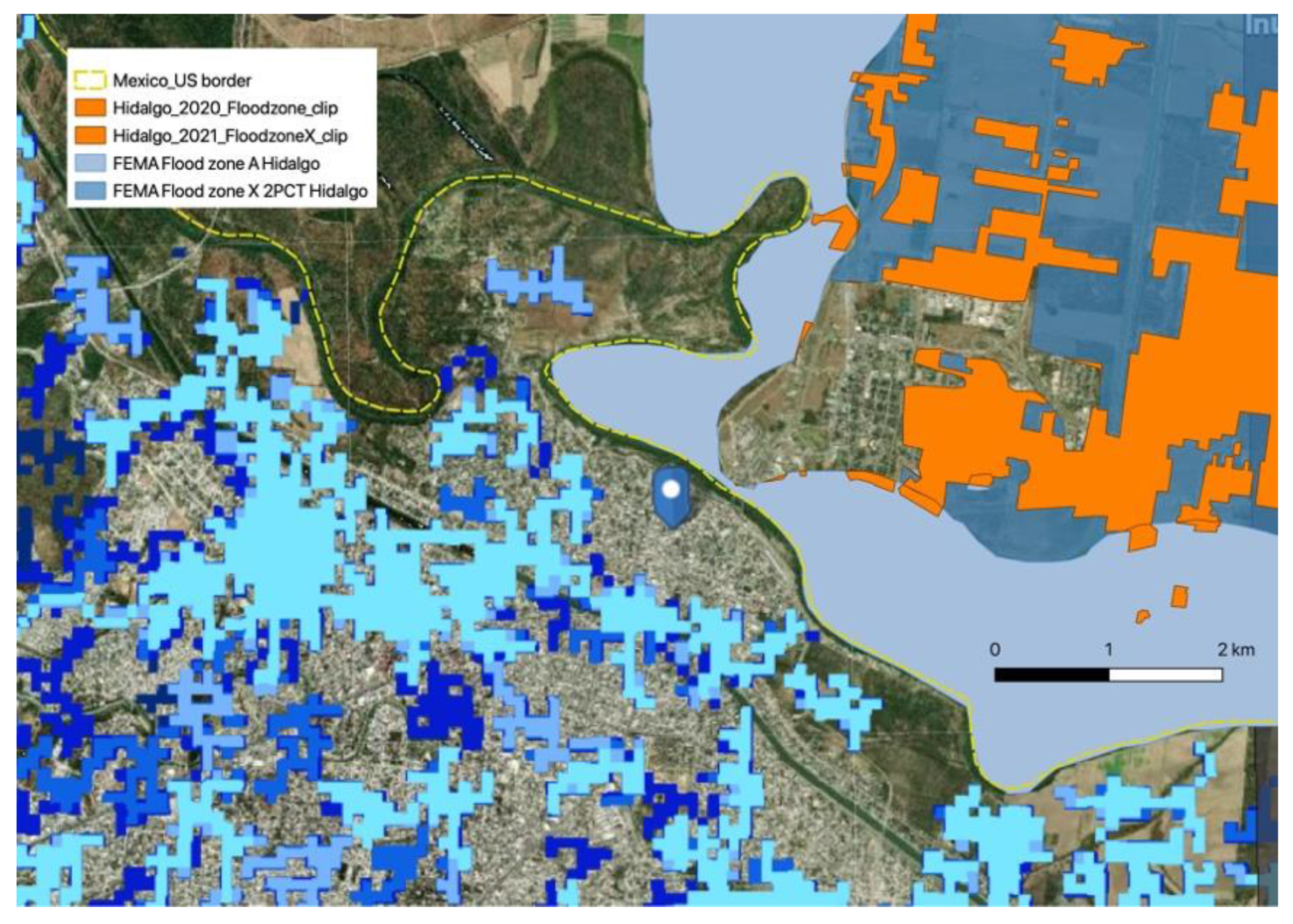
Some additional limitations need to be described for fellow researchers or international bodies interested in monitoring urban growth disaster risk. First, it was not easy to identify data for both countries for all aspects. In some categories, such as old aerial or satellite imagery, this is not surprising. Moreover, this is not the only case where studies using remote sensing and other data are hampered by data scarcity [93,94]. We were a bit surprised about the lack of cross-border studies, lack of public repositories of georectified imagery, urban boundary shapefiles, or urban population data in the past. Some cross-border assessments have found solutions for data gaps, however [95]. Nevertheless, it cannot be forgotten to state how laudable both countries provide public data; the US and also Mexico are forerunners and made this assessment possible for outsiders in the first place. Still, the assessment revealed some constraints for international researchers, such as the problem of identifying hazard or vulnerability data that can directly be compared. For example, the flood zones provided by the US CDC and FEMA on an open platform is paralleled by the Mexican government and their Atlas with similar flood hazard and social vulnerability data. Both repositories are excellent, but the SVI is composed of different variables, and the flood zones in Mexico are calculated and provided in a different format and for different types of floods; not as a GIS file and based on a different computation approach that makes it difficult to compare with the US data (Figure 6).
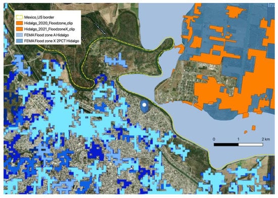
Figure 6.
Hidalgo urban area (orange) exposed to floods in 2020. Note that flood hazard mapping styles and methods differ between Mexico (Atlas Gob) and the USA (FEMA). See Table A2 for data sources.
Availability of public spatial data sources and repositories is still a gap, even more so for most other countries, or even continents, Africa especially [96,97]. Land surveyors and flood risk analysts have much more detailed knowledge and care taken during mapping than we have conducted here. They will also often have done ground-truthing by fieldwork. Drone-truthing could be a promising future alternative [98]. However, many aerial images are not available for public usage, especially when georectified. Maintaining public data repositories such as those used here is important to support, and hopefully, more data will become available for long-term monitoring. This would ideally include urban boundary mapping at regular intervals as well as hazard zones or vulnerability information.
There appear to exist relatively few studies on urban growth or flood risk in these Mexican-US border cities using spatial assessments. There are studies on each city, often by similar author groups who seem to have an individual interest, yet overview studies on several cities are still missing. There are, however, change detection studies using remote sensing for twin cities [99,100] or multi-cities [101] in other regions. Cross-border SVI or flood risk mapping using cities or county units at the cross-regional level could be an interesting upcoming research field.
5.2. Opportunities by Exploring Old Aerial and Satellite Imagery—Urban Growth into Hazard Areas Detected by Comparison to the Previous Land Surface
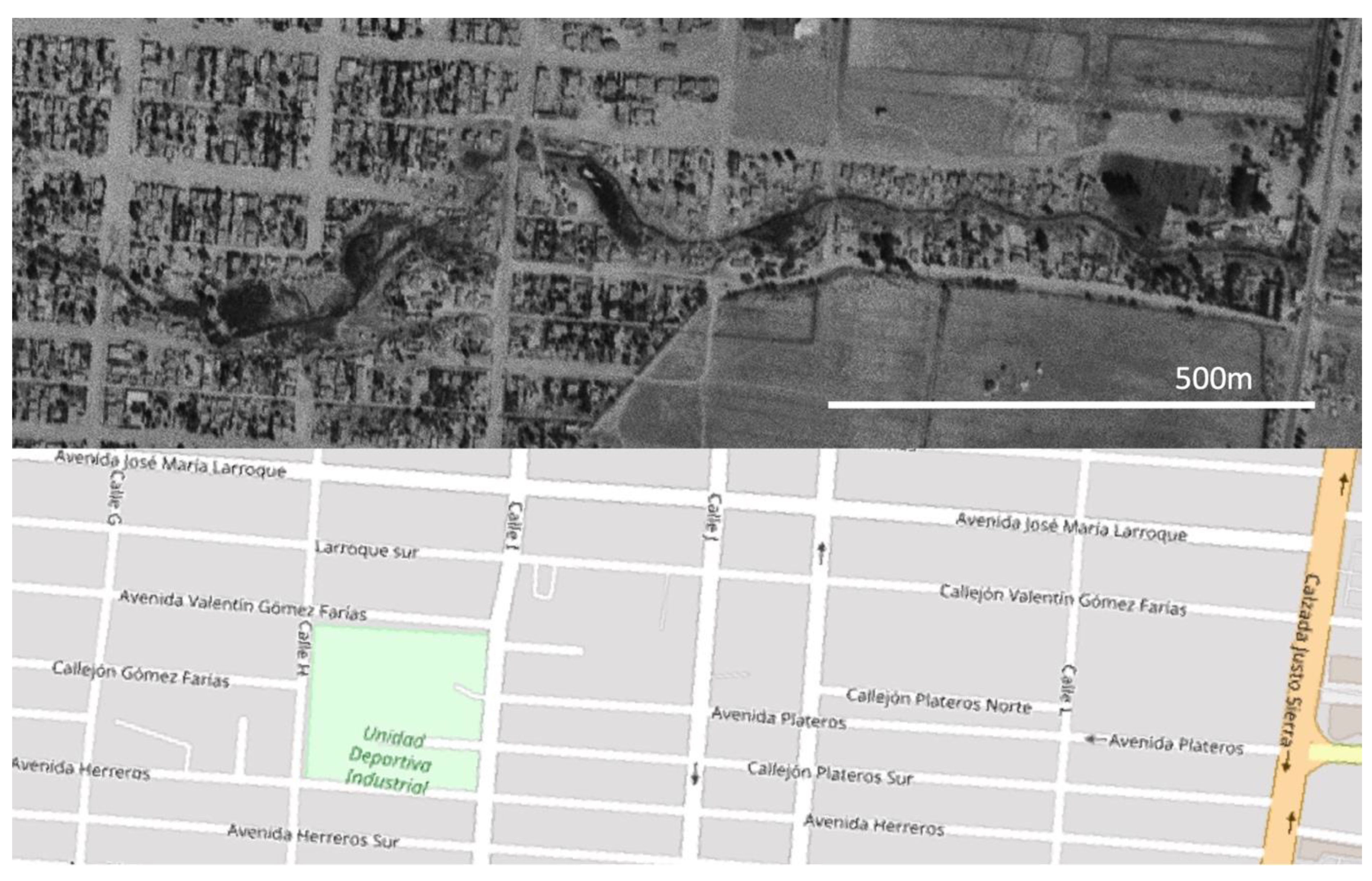
Old declassified espionage satellite imagery such as CORONA seems hardly been used for urban growth in conjunction with disaster risk or hazard mapping [102]. For this study, no examples were identified (see search term list in Table A1). Aerial imagery also is hardly used, even when it ranges back much further. One major advantage is that such old data are often the only witnesses of former land cover at such a scale. This enables capturing former natural environments that can indicate recent natural hazards, such as riverine floods or landslides. Urban growth and river training have often massively changed the land use of former river beds (Figure 7). While flood damage has been reduced according to the engineered safety level, history has proven early on that human adjustment to hazards is limited [103], for example, when extreme floods take old river beds in.
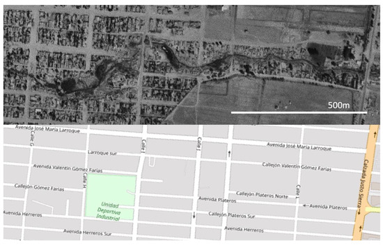
Figure 7.
Mexicali 1953 on the aerial image (above) and 2021 on the OSM map (below) show an old river covered by a settlement area.
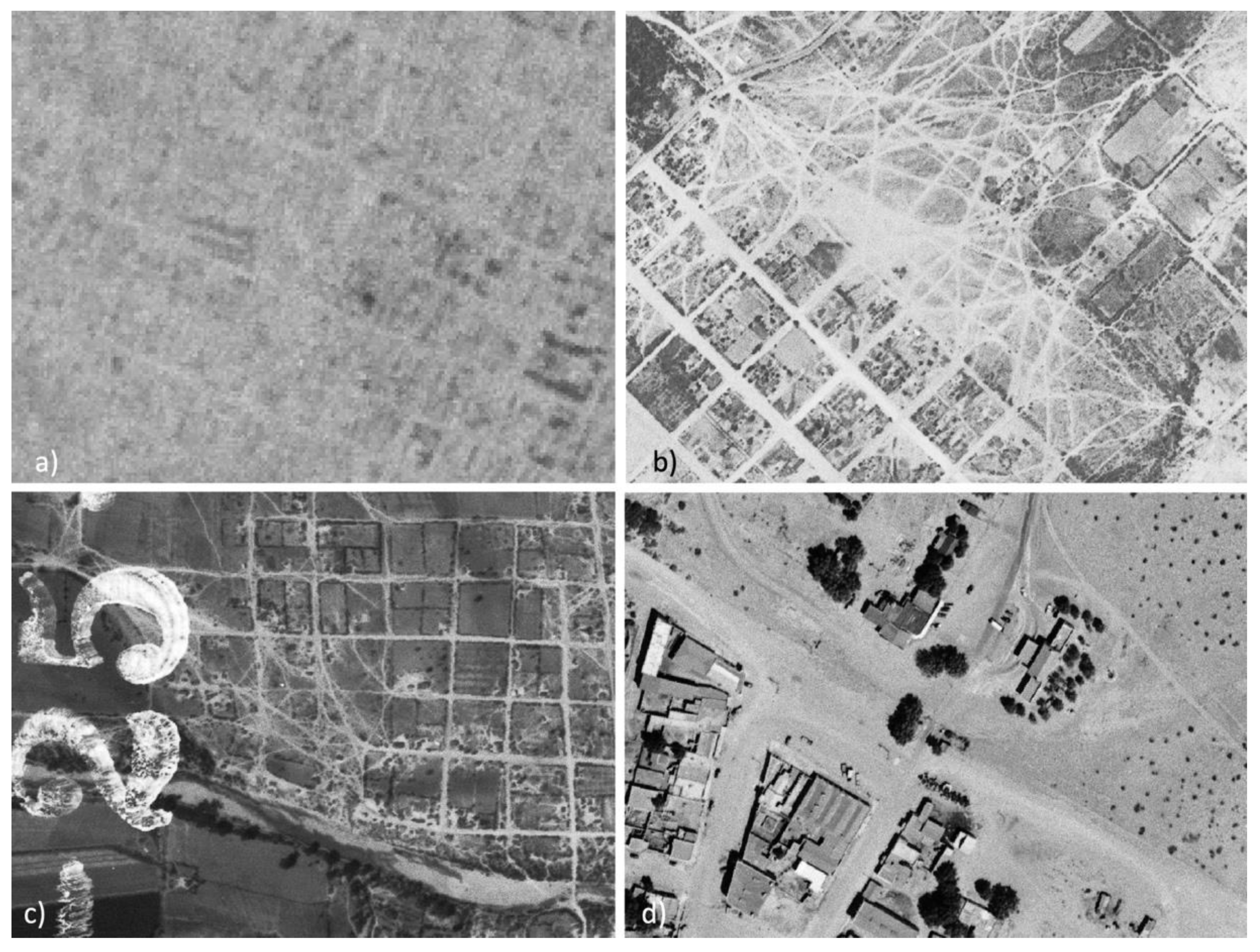
However, certain limitations of spatial resolution or specific aspects of film satellite data also have to be mentioned. This is in terms of transparency to inform other studies on constraints for applications in other areas. For example, the spatial resolution of some of the CORONA satellite images constrains urban feature identification [104]. Of course, this can be the case for aerial images of low resolution just as well [105]. Figure 8a is an example where mapping has become difficult due to the constraints in spatial resolution and greyscale depth. We also identified this to be a constraint for automatized classification. The image in Figure 8a is an aerial image with an original spatial scale of 1:130,000. The higher resolution of the other three aerial images in Figure 8 is due to a better spatial scale of 1:46,000. This enables better identification of objects such as streets and buildings Figure 8b,d). At a viewing scale of 1:2500, individual land plots, streets, houses, and trees can be identified and mapped (Figure 8a–c), but zooming in more can reveal even more details when the resolution permits (Figure 8d). Markings at the margins at the aerial images (Figure 8c) or lower resolution at the corners due to lens distortions can be a constraint, too. The national border itself can be difficult to identify when border fences were not established yet, and border posts such as in San Luis were still very small (Figure 8d).

Figure 8.
Four examples and close-ups of aerial images used and their original mapping resolutions; (a) Ciudad Juarez 1956 1:130,000, (b) 1950 Del Rio 1:46,000, (c) 1950 Ciudad Acuna 1:46,000, (d) San Luis 1946 1:12,000.
6. Conclusions
This study replied to the main research question guiding this article, “How did Mexican-US border cities develop over time and concerning flood hazards?” by providing a mapping and statistical comparison of 23 cities. The findings show that the border is a zone where urban growth is high in both population and area growth, but flood hazard exposure zones have also grown. Furthermore, growth and vulnerability develop heterogeneously within each country, but especially between sister cities on both sides. In Mexico, it seems that more cities have grown at a more rapid pace than their US counterparts, and the border stands out as a stark visual demarcation when mapped from space.
Based on the literature review conducted, this appears to be one of the first studies to compare that many cross-border cities along the Mexican-US border by capturing both urban growth and flood exposure while ranging back to the 1940s. Thereby it addresses an important data gap in change detection assessments. The results look promising to expand this study and conduct similar assessments along other national and natural borders. This paper demonstrates how old aerial images and satellite data can be used to expand the temporal assessment of urban growth. State-of-the-art spatial assessments often rely on Landsat data, which only ranges back to the early 1970s and provides much coarser spatial resolution. While limited by their grayscale information, they are often unique to providing information about the previous land cover before settlement.
As an outlook, the findings also demonstrate the challenges for international bodies such as the Sendai monitoring process to conduct long-term spatial risk assessments. It seems necessary to thank those institutions for maintaining public data repositories as used here. At the same time, this calls for more public data platforms in other areas and countries and expanding exiting platforms on georectified images and urban border shapefiles. Finally, using the same set of core variables for similar social vulnerability or resilience assessments and using the same classes would be great for transboundary comparisons. This is important not only for flood hazards but also for other hazards in the region, such as hurricanes that can force people to evacuate, which underlines the demand for better informed decision-making [106]. Another area is migration which can suddenly develop into an additional humanitarian conflict, as recently has been shown and where remoter sensing information also helped to survey the situation [9]. The combination of such risks is increasingly becoming a research topic, for example, under the terms ‘multi-risk assessment’ [107,108,109,110], ‘cascading effects’ [111,112,113], or ‘compounding events’ [114,115]. These are all areas in high demand of big data and where remote sensing studies can help provide baseline data for monitoring hazard areas and dynamical developments leading to an increase in risk.
Author Contributions
Conceptualization, A.F.; methodology, A.F.; software, A.F. and P.P.; formal analysis, A.F.; investigation, A.F. and P.P.; data curation, A.F. and P.P.; writing—original draft preparation, A.F.; writing—review and editing, A.F. and P.P.; visualization, A.F. and P.P. All authors have read and agreed to the published version of the manuscript.
Funding
This research received no external funding.
Data Availability Statement
We host data we have developed such as urban coverage, or georectified imagery at our open data repository at: (https://riskncrisis.wordpress.com/data accessed on 31 October 2021).
Conflicts of Interest
The authors declare no conflict of interest.
Appendix A

Table A1.
List of search terms used.
Table A1.
List of search terms used.
| Search Term | Search Engine | Date of Search | Comment |
|---|---|---|---|
| social vulnerability index mexico | Google Scholar | 18 April 2021 | |
| mexico vulnerabilidad social | Google Scholar | 18 April 2021 | |
| mexico USA border cities flood | Google Scholar | 18 April 2021 | |
| Urban growth border Mexic | Google Scholar | 18 April 2021 | Many hits |
| Urban sprawl border Mexic | Google Scholar | 20 April 2021 | Very few additional hits |
| Urban sprawl border Mexic remote sensing | Google Scholar | 20 April 2021 | Few additional hits |
| border Mexic “CORONA satellite” | Google Scholar | 20 April 2021 | No significant hits |
| Mexic border flood analysis | Google Scholar | 20 April 2021 | Very few additional hits |
| Urban growth (city name) remote sensing | Google Scholar | 20 April 2021 | Some hits |
| Urban growth (city name) | Google Scholar | 20 April 2021 | Few relevant hits |
| Urban growth OR sprawl OR expansion (city name) | Google Scholar | 20 April 2021 | Few relevant hits |
| Urban growth OR sprawl OR expansion (city name) remote sensing | Google Scholar | 20 April 2021 | Few relevant hits |
| City name AND flood | Google Scholar | 2 May 2021 | Hits depending on city |
| City name AND flood map OR flood plain | Google Scholar | 3 May 2021 | |
| City name AND flood map | 3 May 2021 | ||
| City name ANDinundación OR aluvión AND mapa | 3 May 2021 | ||
| Cross-border flood risk map | Google Scholar | 15 May 2021 | Few hits, mostly for European cross-border river basins |
| Zonas de riesgo por desbordamiento | 20 May 2021 | Works for some cities |

Table A2.
List of data used.
Table A2.
List of data used.
| Description | File Type | Provider/Author | File Name | File Date | Access Date | Link |
|---|---|---|---|---|---|---|
| Admin. boundaries, municipios Mexico | Shapefile | CONABIO | División política municipal, 1:250000. 2018 | 10 Feb 2021 | 13 May 2021 | http://www.conabio.gob.mx/informacion/gis/ |
| SVI 2010 Mexico | Shapefile | CONABIO | Grado de vulnerabilidad social por municipio, 2010 | 10 Feb 2021 | 13 May 2021 | http://www.conabio.gob.mx/informacion/gis/ |
| Flood risk MX | Shapefile | CONABIO/CENAPRED | Grado de riesgo por inundaciones por municipio | 12 Sep 2007 | 13 May 2021 | http://www.conabio.gob.mx/informacion/gis/ |
| Rivers_MX | Shapefile | CONABIO/Maderey-R, L. E. y Torres-Ruata, C. | Hidrografía | 1990 | 13 May 2021 | http://www.conabio.gob.mx/informacion/gis/ |
| SVI 2010 USA | Geodatabase | CDC | CDC/ATSDR SVI Data and Documentation Download. Counties or Census tract (RPL_Themes) | 2010, 2018 | 13,26 May 2021 | https://www.atsdr.cdc.gov/placeandhealth/svi/data_documentation_download.html |
| Admin boundaries, counties, USA | US census/MAF/TIGER | County and Equivalent | 2020 | 13 May 2021 | https://www.census.gov/geographies/mapping-files/time-series/geo/carto-boundary-file.html | |
| Floodzones USA | Shapefile | FEMA’s National Flood Hazard Layer (NFHL) Viewer | FEMA’s National Flood Hazard Layer (NFHL) Viewer/S_FLD_HAZ_AR.shp | varies | 13 May 2021 | https://hazards-fema.maps.arcgis.com/apps/webappviewer/index.html?id=8b0adb51996444d4879338b5529aa9cd |
| Floodzones Mexico | KMZ | Gobierno de Mexico/CENAPRED | Atlas Nacional de Riesgos por Inundacion (ANRI) | 13 May 2021 | http://atlasnacionalderiesgos.gob.mx/archivo/visor-capas.html | |
| Aerial images; CORONA satellite date | TIFF | USGS Earth Explorer | Aerial Photo Single Frames; Declassified Data | varies | 1 December 2020–31 May 2021 | https://earthexplorer.usgs.gov |
| Basemap | WMS | Open Street Map | 1 December 2020 | https://tile.openstreetmap.org/ | ||
| Sentinel 2 satellite data | WMS | EOX::Maps | Sentinel-2 cloudless layer for 2020 by EOX-4326 | 2020 | 20 April 2021 | https://tiles.maps.eox.at/wms? |
| Border, US states | Shapefile | US census/MAF/TIGER | State and Equivalent | 2020 | 14 May 2021 | https://www.census.gov/geographies/mapping-files/time-series/geo/carto-boundary-file.html |
| Border encounters | Table | US Customs and Border Protection | Southwest Land Border Encounters (By Component) | 2021 | 14 May 2021 | https://www.cbp.gov/newsroom/stats/southwest-land-border-encounters-by-component |

Table A3.
SVI at census tract level in the USA.
Table A3.
SVI at census tract level in the USA.
| City in USA | SVI 2010 (Municipium/Counties) | SVI Change (2000–2010) | SVI 2018 Census Tract (Mean Value) * | SVI Census Tract (Min) | SVI Census Tract (Max) |
|---|---|---|---|---|---|
| San Ysidro | high | no change | 0.803 | 0.412 | 0.993 |
| Imperial Beach city | high | no change | 0.650 | 0.050 | 0.978 |
| Calexico | highest | no change | 0.923 | 0.770 | 0.995 |
| San Luis | highest | no change | 0.837 | 0.745 | 0.958 |
| Nogales | highest | no change | 0.927 | 0.655 | 0.998 |
| Douglas | highest | no change | 0.902 | 0.773 | 0.990 |
| El Paso | highest | no change | 0.686 | 0.051 | 1.000 |
| Del Rio | highest | no change | 0.794 | 0.549 | 0.974 |
| Eagle Pass | highest | no change | 0.916 | 0.801 | 0.990 |
| Laredo | highest | no change | 0.825 | 0.297 | 1.000 |
| Hidalgo | highest | no change | 0.887 | 0.752 | 0.975 |
* false entries removed, such as −999 (airports etc.)
References
- UN/HABITAT. New urban agenda. In Proceedings of the United Nations, Habitat III Secretariat, Quito, Ecuador, 20 October 2016; p. 65. [Google Scholar]
- United Nations. Sendai Framework for Disaster Risk Reduction 2015–2030; United Nations Office for Disaster Risk Reduction: Geneva, Switzerland, 2015. [Google Scholar]
- Bogardi, J.J. Hazards, risks and vulnerabilities in a changing environment: The unexpected onslaught on human security? Glob. Environ. Chang. 2004, 14, 361–365. [Google Scholar] [CrossRef]
- Guadagno, L. Human Mobility in the Sendai Framework for Disaster Risk Reduction. Int. J. Disaster Risk Sci. 2016, 7, 30–40. [Google Scholar] [CrossRef] [Green Version]
- Warner, K.; Hamza, M.; Oliver-Smith, A.; Renaud, F.; Julca, A. Climate change, environmental degradation and migration. Nat. Hazards 2010, 55, 689–715. [Google Scholar] [CrossRef]
- Wachtendorf, T. When Disaster Defy Borders: What We can Learn from the Red River Flood about Transnational Disasters. Aust. J. Emerg. Manag. 2000, 15, 36–41. [Google Scholar]
- Berchtold, C.; Vollmer, M.; Sendrowski, P.; Neisser, F.; Müller, L.; Grigoleit, S. Barriers and Facilitators in Interorganizational Disaster Response: Identifying Examples Across Europe. Int. J. Disaster Risk Sci. 2020, 11, 46–58. [Google Scholar] [CrossRef] [Green Version]
- Hannigan, J. Disasters across borders: Borderlands as spaces of hope and innovation in the geopolitics of environmental disasters. In Crossing Borders: Governing Environmental Disasters in a Global Urban Age in Asia and the Pacific; Miller, M.A., Douglass, M., Garschagen, M., Eds.; Springer: Singapore, 2018; pp. 79–94. [Google Scholar]
- Chute, N. See Drone Footage, Satellite Images Showing Thousands of Haitian Migrants Gathered at Del Rio Border. Available online: https://eu.elpasotimes.com/story/news/2021/09/20/del-rio-bridge-drone-video-texas-border-photos-haiti-migrants/8418312002/ (accessed on 22 October 2021).
- Roberts, K. Haitians Under Its Bridge, Del Rio Ranks Among Top 25% of Nation’s Trade Gateways. Available online: https://www.forbes.com/sites/kenroberts/2021/09/22/haitians-under-its-bridge-del-rio-ranks-among-top-25-of-nations-trade-gateways/?sh=1164daec1847 (accessed on 22 October 2021).
- Villarreal, A. ‘Sleeping in the Dust’: Migrants Face Harsh Conditions in Del Rio as 5000 Remain. Available online: https://www.theguardian.com/us-news/2021/sep/24/haitian-migrants-del-rio-border-camp (accessed on 22 October 2021).
- Flanagan, B.E.; Hallisey, E.J.; Adams, E.; Lavery, A. Measuring community vulnerability to natural and anthropogenic hazards: The Centers for Disease Control and Prevention’s Social Vulnerability Index. J. Environ. Health 2018, 80, 34. [Google Scholar]
- Gobierne De México. Atlas Nacional De Riesgos. Indicadores. Grado De Vulnerabilidad Social (Indicadores Socioeconómicos). Available online: http://atlasnacionalderiesgos.gob.mx/archivo/visor-capas.html (accessed on 1 October 2021).
- Mueller, E.R.; Schmidt, J.C.; Topping, D.; Grams, P.E. Geomorphic change in the limitrophe reach of the Colorado River in response to the 2014 delta pulse flow, United States and Mexico. In Proceedings of the SEDHYD 2015, Reno, NV, USA, 19–23 April 2015. [Google Scholar]
- Sadasivam, N. Fenced in and Flooded out. The US-Mexico Border Wall’s Dangerous, Costly Side-Effect: Enormous Floods. Available online: https://qz.com/1353798/the-us-mexico-border-walls-dangerous-costly-side-effect-enormous-floods/ (accessed on 1 November 2021).
- Norman, L.M.; Huth, H.; Levick, L.; Shea Burns, I.; Phillip Guertin, D.; Lara-Valencia, F.; Semmens, D. Flood hazard awareness and hydrologic modelling at Ambos Nogales, United States–Mexico border. J. Flood Risk Manag. 2010, 3, 151–165. [Google Scholar] [CrossRef]
- Bagan, H.; Yamagata, Y. Landsat analysis of urban growth: How Tokyo became the world’s largest megacity during the last 40years. Remote Sens. Environ. 2012, 127, 210–222. [Google Scholar] [CrossRef]
- Masek, J.; Lindsay, F.; Goward, S. Dynamics of urban growth in the Washington DC metropolitan area, 1973–1996, from Landsat observations. Int. J. Remote Sens. 2000, 21, 3473–3486. [Google Scholar] [CrossRef]
- Song, X.-P.; Sexton, J.O.; Huang, C.; Channan, S.; Townshend, J.R. Characterizing the magnitude, timing and duration of urban growth from time series of Landsat-based estimates of impervious cover. Remote Sens. Environ. 2016, 175, 1–13. [Google Scholar] [CrossRef]
- Asadzadeh, A.; Kötter, T.; Weiss, D. The multi-scale patterns of urban disaster resilience: Case study of Tehran City, Iran. In Proceedings of the Extended Abstract. IDRC DAVOS 2016 “Integrative Risk Management—Towards Resilient Cities”, Davos, Switzerland, 28 August–1 September 2016; pp. 62–65. [Google Scholar]
- Contreras Mojica, D.M.; Chamorro, A. A socio-economic vulnerability to natural hazards: A spatial model including dependencies to critical urban infrastructure. In Proceedings of the Deutscher Kongress für Geographie 2019, Kiel, Germany, 25 September–1 October 2019. [Google Scholar]
- Kraff, N.J.; Wurm, M.; Taubenböck, H. The dynamics of poor urban areas-analyzing morphologic transformations across the globe using Earth observation data. Cities 2020, 107, 102905. [Google Scholar] [CrossRef]
- Bayram, B.; Bayraktar, H.; Helvaci, C.; Acar, U. Coastline change detection using CORONA, SPOT and IRS 1D images. Int. Arch. Photogramm. Remote Sens. 2004, 35, 437–441. [Google Scholar]
- Bolch, T.; Buchroithner, M.; Pieczonka, T.; Kunert, A. Planimetric and volumetric glacier changes in the Khumbu Himal, Nepal, since 1962 using Corona, Landsat TM and ASTER data. J. Glaciol. 2008, 54, 592–600. [Google Scholar] [CrossRef] [Green Version]
- Narama, C.; Kääb, A.; Duishonakunov, M.; Abdrakhmatov, K. Spatial variability of recent glacier area changes in the Tien Shan Mountains, Central Asia, using Corona (~1970), Landsat (~2000), and ALOS (~2007) satellite data. Glob. Planet. Chang. 2010, 71, 42–54. [Google Scholar] [CrossRef]
- Song, D.-X.; Huang, C.; Sexton, J.O.; Channan, S.; Feng, M.; Townshend, J.R. Use of Landsat and Corona data for mapping forest cover change from the mid-1960s to 2000s: Case studies from the Eastern United States and Central Brazil. ISPRS J. Photogramm. Remote Sens. 2015, 103, 81–92. [Google Scholar] [CrossRef] [Green Version]
- Tappan, G.G.; Hadj, A.; Wood, E.C.; Lietzow, R.W. Use of Argon, Corona, and Landsat imagery to assess 30 years of land resource changes in west-central Senegal. Photogramm. Eng. Remote Sens. 2000, 66, 727–736. [Google Scholar]
- Stewart, D.J.; Yin, Z.-Y.; Bullard, S.M.; MacLachlan, J.T. Assessing the spatial structure of urban and population growth in the Greater Cairo area, Egypt: A GIS and imagery analysis approach. Urban Stud. 2004, 41, 95–116. [Google Scholar] [CrossRef]
- Cecchini, M.; Zambon, I.; Pontrandolfi, A.; Turco, R.; Colantoni, A.; Mavrakis, A.; Salvati, L. Urban sprawl and the ‘olive’landscape: Sustainable land management for ‘crisis’ cities. GeoJournal 2019, 84, 237–255. [Google Scholar] [CrossRef]
- Hepcan, S.; Hepcan, C.C.; Kilicaslan, C.; Ozkan, M.B.; Kocan, N. Analyzing landscape change and urban sprawl in a Mediterranean coastal landscape: A case study from Izmir, Turkey. J. Coast. Res. 2013, 29, 301–310. [Google Scholar]
- Moghadas, M.; Asadzadeh, A.; Vafeidis, A.; Fekete, A.; Ktter, T. A multi-criteria approach for assessing urban flood resilience in Tehran, Iran. Int. J. Disaster Risk Reduct. 2019, 35, 101069. [Google Scholar] [CrossRef]
- Criado, M.; Santos-Francés, F.; Martínez-Graña, A.; Sánchez, Y.; Merchán, L. Multitemporal Analysis of Soil Sealing and Land Use Changes Linked to Urban Expansion of Salamanca (Spain) Using Landsat Images and Soil Carbon Management as a Mitigating Tool for Climate Change. Remote Sens. 2020, 12, 1131. [Google Scholar] [CrossRef] [Green Version]
- UNISDR. Technical Guidance for Monitoring and Reporting on Progress in Achieving the Global Targets of the Sendai Framework for Disaster Risk Reduction, New ed.; United Nations: Geneva, Switzerland, 2017; p. 179. [Google Scholar]
- Taubenböck, H.; Esch, T.; Wurm, M.; Thiel, M.; Ullmann, T.; Roth, A.; Schmidt, M.; Mehl, H.; Dech, S. Urban structure analysis of mega city Mexico City using multisensoral remote sensing data. In Proceedings of the Remote Sensing for Environmental Monitoring, GIS Applications, and Geology VIII, Cardiff, Wales, 16 September 2008; p. 71100E. [Google Scholar]
- Cutter, S.L.; Emrich, C.T.; Morath, D.P.; Dunning, C.M. Integrating social vulnerability into federal flood risk management planning. J. Flood Risk Manag. 2013, 6, 332–344. [Google Scholar] [CrossRef]
- Chatfield, W.H. The Twin Cities (Brownsville, Texas; Matamoros, Mexico) of the Border and the Country of the Lower Rio Grande; Harbert Davenport Memorial Fund, E.P. Brandao: New Orleans, LA, USA, 1893. [Google Scholar]
- Dillman, C.D. Border Town Symbiosis Along the Lower Rio Grande as Exemplified by the Twin Cities, Brownsville, Texas and Matamoros, Tamaulipas. Rev. Geográfica 1969, 71, 93–113. [Google Scholar]
- Dillman, C.D. Urban growth along Mexico’s northern border and the Mexican national border program. J. Dev. Areas 1970, 4, 487–508. [Google Scholar]
- Arbeláez, M.S.; Arreola, D.D.; De Baca, J.C.; De Baca, V.C.; Du Bry, T.; Hayman, J.M.; Macías-González, V.M.; Pilcher, J.M.; Schantz, E.M.; Taylor, L.D. On the Border: Society and Culture between the United States and Mexico; Rowman & Littlefield Publishers: Lanham, MD, USA, 2004. [Google Scholar]
- Herzog, L.A. Where North Meets South: Cities, Space, and Politics on the United States-Mexico Border; University of Texas: Richardson, TX, USA, 1990. [Google Scholar]
- Peña, S. Recent developments in urban marginality along Mexico’s northern border. Habitat Int. 2005, 29, 285–301. [Google Scholar] [CrossRef]
- Zhao, C.; Jensen, J.; Zhan, B. A comparison of urban growth and their influencing factors of two border cities: Laredo in the US and Nuevo Laredo in Mexico. Appl. Geogr. 2017, 79, 223–234. [Google Scholar] [CrossRef]
- Zhao, C.; Jensen, J.L.R.; Weaver, R. Global and Local Modeling of Land Use Change in the Border Cities of Laredo, Texas, USA and Nuevo Laredo, Tamaulipas, Mexico: A Comparative Analysis. Land 2020, 9, 347. [Google Scholar] [CrossRef]
- Biggs, T.W.; Atkinson, E.; Powell, R.; Ojeda-Revah, L. Land cover following rapid urbanization on the US–Mexico border: Implications for conceptual models of urban watershed processes. Landsc. Urban Plan. 2010, 96, 78–87. [Google Scholar] [CrossRef]
- Norman, L.M.; Feller, M.; Phillip Guertin, D. Forecasting urban growth across the United States–Mexico border. Comput. Environ. Urban Syst. 2009, 33, 150–159. [Google Scholar] [CrossRef]
- Myint, S.W.; Jain, J.; Lukinbeal, C.; Lara-Valencia, F. Simulating urban growth on the US-Mexico border: Nogales, Arizona, and Nogales, Sonora. Can. J. Remote Sens. 2010, 36, 166–184. [Google Scholar] [CrossRef]
- Sánchez Rodríguez, R.A.; Morales Santos, A.E. Vulnerability assessment to climate variability and climate change in Tijuana, Mexico. Sustainability 2018, 10, 2352. [Google Scholar] [CrossRef]
- Mubako, S.; Belhaj, O.; Heyman, J.; Hargrove, W.; Reyes, C. Monitoring of land use/land-cover changes in the arid transboundary middle Rio grande basin using remote sensing. Remote Sens. 2018, 10, 2005. [Google Scholar] [CrossRef] [Green Version]
- Leyva-Camacho, O.; Venegas-Cardoso, R.; Rojas-Caldelas, R.; Ranfla-Gonzalez, A.; Pena-Salmon, C. Urban expansion and change of land uses: City of Mexicali 1990–2005. WIT Trans. Ecol. Environ. 2010, 129, 547–558. [Google Scholar]
- Norman, L.; Donelson, A.J.; Pfeifer, E.L.; Lam, A.H.; Osborn, K.J. Monitoring colonias development along the United States–Mexico border: A process application using GIS and remote sensing in Douglas, Arizona, and Agua Prieta, Sonora. USGS Menlo Park USGS Open-File Rep. 2004, 1212, 1–100. [Google Scholar]
- Korbulic, Q.P. Tracking Urban Growth and Composition along the Western Portion of the US-Mexico Border: 1985–2010. 2012. Available online: https://scholarworks.unr.edu/bitstream/handle/11714/3611/Korbulic_unr_0139D_10991.pdf?sequence=1&isAllowed=y (accessed on 1 November 2021).
- Peña, E.N. Using Census Data, Urban Land-Cover Classification, and Dasymetric Mapping to Measure Urban Growth of the Lower Rio Grande Valley, Texas; University of Southern California: Los Angeles, CA, USA, 2012; p. 46. [Google Scholar]
- Leigh, E.; Barroso, M.; Fipps, G. Expansion of Urban Area in Irrigation Districts of the Rio Grande River Basin, 1996–2006: A Map Series. Available online: https://oaktrust.library.tamu.edu/handle/1969.1/94956 (accessed on 22 October 2021).
- Bohn, T.J.; Vivoni, E.R.; Mascaro, G.; White, D.D. Land and water use changes in the US–Mexico border region, 1992–2011. Environ. Res. Lett. 2018, 13, 114005. [Google Scholar] [CrossRef] [Green Version]
- Wilder, M.; Scott, C.A.; Pablos, N.P.; Varady, R.G.; Garfin, G.M.; McEvoy, J. Adapting Across Boundaries: Climate Change, Social Learning, and Resilience in the U.S.–Mexico Border Region. Ann. Assoc. Am. Geogr. 2010, 100, 917–928. [Google Scholar] [CrossRef]
- Tiefenbacher, J.P. The Role of Internacional Boundaries in Flood Hazard, Social Vulnerability and Disaster: A Bi-National Case Study of Ciudad Acuña, Coahuila and Del Rio, Texas. Nóesis Rev. De Cienc. Soc. Y Humanid. 2006, 15, 68–92. [Google Scholar]
- Bhatta, B. Analysis of Urban Growth and Sprawl from Remote Sensing Data; Springer Science & Business Media: Heidelberg, Germany, 2010. [Google Scholar]
- Patino, J.E.; Duque, J.C. A review of regional science applications of satellite remote sensing in urban settings. Comput. Environ. Urban Syst. 2013, 37, 1–17. [Google Scholar] [CrossRef]
- Maxwell, A.E.; Warner, T.A.; Fang, F. Implementation of machine-learning classification in remote sensing: An applied review. Int. J. Remote Sens. 2018, 39, 2784–2817. [Google Scholar] [CrossRef] [Green Version]
- Stiller, D.; Wurm, M.; Stark, T.; Angelo, P.; Stebner, K.; Dech, S.; Taubenböck, H. Spatial parameters for transportation: A multi-modal approach for modelling the urban spatial structure using deep learning and remote sensing. J. Transp. Land Use 2021, 14, 777–803. [Google Scholar] [CrossRef]
- Di Pilato, A.; Taggio, N.; Pompili, A.; Iacobellis, M.; Di Florio, A.; Passarelli, D.; Samarelli, S. Deep learning approaches to Earth Observation change detection. Remote Sens. 2021, 13, 4083. [Google Scholar] [CrossRef]
- Paola, J.D.; Schowengerdt, R.A. A review and analysis of backpropagation neural networks for classification of remotely-sensed multi-spectral imagery. Int. J. Remote Sens. 1995, 16, 3033–3058. [Google Scholar] [CrossRef]
- Al-Hameedi, W.M.M.; Chen, J.; Faichia, C.; Al-Shaibah, B.; Nath, B.; Kafy, A.-A.; Hu, G.; Al-Aizari, A. Remote Sensing-Based Urban Sprawl Modeling Using Multilayer Perceptron Neural Network Markov Chain in Baghdad, Iraq. Remote Sens. 2021, 13, 4034. [Google Scholar] [CrossRef]
- Sheykhmousa, M.; Mahdianpari, M.; Ghanbari, H.; Mohammadimanesh, F.; Ghamisi, P.; Homayouni, S. Support vector machine vs. random forest for remote sensing image classification: A meta-analysis and systematic review. IEEE J. Sel. Top. Appl. Earth Obs. Remote Sens. 2020, 13, 6308–6325. [Google Scholar] [CrossRef]
- Mountrakis, G.; Im, J.; Ogole, C. Support vector machines in remote sensing: A review. ISPRS J. Photogramm. Remote Sens. 2011, 66, 247–259. [Google Scholar] [CrossRef]
- Qiming, Z. Review on Change detection using multi-temporal remotely sensed imagery. Geomat. World 2011, 9, 28–33. [Google Scholar]
- Plank, S. Rapid damage assessment by means of multi-temporal SAR—A comprehensive review and outlook to Sentinel-1. Remote Sens. 2014, 6, 4870–4906. [Google Scholar] [CrossRef] [Green Version]
- Brito, P.; Quintanilha, J. A literature review, 2001–2008, of classification methods and inner urban characteristics identified in multispectral remote sensing images. In Proceedings of the 4th GEOBIA, Rio de Janeiro, Brazil, 7–9 May 2012; pp. 586–591. [Google Scholar]
- Hong, D.; Gao, L.; Yokoya, N.; Yao, J.; Chanussot, J.; Du, Q.; Zhang, B. More Diverse Means Better: Multimodal Deep Learning Meets Remote-Sensing Imagery Classification. IEEE Trans. Geosci. Remote Sens. 2021, 59, 4340–4354. [Google Scholar] [CrossRef]
- Acevedo, W.; Masuoka, P. Time-series animation techniques for visualizing urban growth. Comput. Geosci. 1997, 23, 423–435. [Google Scholar] [CrossRef]
- Li, X.; Zhou, Y.; Zhu, Z.; Liang, L.; Yu, B.; Cao, W. Mapping annual urban dynamics (1985–2015) using time series of Landsat data. Remote Sens. Environ. 2018, 216, 674–683. [Google Scholar] [CrossRef]
- Lawton, M.N.; Martí-Cardona, B.; Hagen-Zanker, A. Urban Growth Derived from Landsat Time Series Using Harmonic Analysis: A Case Study in South England with High Levels of Cloud Cover. Remote Sens. 2021, 13, 3339. [Google Scholar] [CrossRef]
- Ghassemian, H. A review of remote sensing image fusion methods. Inf. Fusion 2016, 32, 75–89. [Google Scholar] [CrossRef]
- Bai, L.; Xu, C.; Wang, C. A review of fusion methods of multi-spectral image. Optik 2015, 126, 4804–4807. [Google Scholar] [CrossRef]
- Pohl, C.; Van Genderen, J.L. Review article multisensor image fusion in remote sensing: Concepts, methods and applications. Int. J. Remote Sens. 1998, 19, 823–854. [Google Scholar] [CrossRef] [Green Version]
- Gao, L.; Hong, D.; Yao, J.; Zhang, B.; Gamba, P.; Chanussot, J. Spectral superresolution of multispectral imagery with joint sparse and low-rank learning. IEEE Trans. Geosci. Remote Sens. 2020, 59, 2269–2280. [Google Scholar] [CrossRef]
- Blaschke, T. Object based image analysis for remote sensing. ISPRS J. Photogramm. Remote Sens. 2010, 65, 2–16. [Google Scholar] [CrossRef] [Green Version]
- Kucharczyk, M.; Hay, G.J.; Ghaffarian, S.; Hugenholtz, C.H. Geographic object-based image analysis: A primer and future directions. Remote Sens. 2020, 12, 2012. [Google Scholar] [CrossRef]
- Soergel, U. Review of radar remote sensing on urban areas. In Radar Remote Sensing of Urban Areas; Springer: Dordrecht, The Netherlands, 2010; pp. 1–47. [Google Scholar]
- Yan, W.Y.; Shaker, A.; El-Ashmawy, N. Urban land cover classification using airborne LiDAR data: A review. Remote Sens. Environ. 2015, 158, 295–310. [Google Scholar] [CrossRef]
- Wedajo, G. LiDAR DEM Data for flood mapping and assessment; opportunities and challenges: A Review. J. Remote Sens. Gis 2017, 6, 2015–2018. [Google Scholar] [CrossRef]
- Wentz, E.A.; Anderson, S.; Fragkias, M.; Netzband, M.; Mesev, V.; Myint, S.W.; Quattrochi, D.; Rahman, A.; Seto, K.C. Supporting global environmental change research: A review of trends and knowledge gaps in urban remote sensing. Remote Sens. 2014, 6, 3879–3905. [Google Scholar] [CrossRef] [Green Version]
- Zhao, M.; Zhou, Y.; Li, X.; Cao, W.; He, C.; Yu, B.; Li, X.; Elvidge, C.D.; Cheng, W.; Zhou, C. Applications of satellite remote sensing of nighttime light observations: Advances, challenges, and perspectives. Remote Sens. 2019, 11, 1971. [Google Scholar] [CrossRef] [Green Version]
- Voogt, J.A.; Oke, T.R. Thermal remote sensing of urban climates. Remote Sens. Environ. 2003, 86, 370–384. [Google Scholar] [CrossRef]
- Glass, C.E. Interpreting Aerial Photographs to Identify Natural Hazards; Elsevier: Amsterdam, The Netherlands, 2013. [Google Scholar]
- Rufat, S.; Tate, E.; Burton, C.G.; Maroof, A.S. Social vulnerability to floods: Review of case studies and implications for measurement. Int. J. Disaster Risk Reduct. 2015, 14, 470–486. [Google Scholar] [CrossRef] [Green Version]
- Tate, E. Social vulnerability indices: A comparative assessment using uncertainty and sensitivity analysis. Nat. Hazards 2012, 63, 325–347. [Google Scholar] [CrossRef]
- Birkmann, J. Measuring Vulnerability to Natural Hazards: Towards Disaster Resilient Societies, 2nd ed.; United Nations University Press: Tokyo, Japan, 2013; p. 460. [Google Scholar]
- Stevens, D. Geospatial Information, Sustainable Development and Decision Making in Developing Countries. In Geoinformation for Development; Zeil, P., Ed.; Herbert Wichmann Verlag: Heidelberg, Germany, 2007. [Google Scholar]
- Zollner, K. United Nations Platform for Space-based Information for Disaster Management and Emergency Response (UN-SPIDER). In Satellite-Based Earth Observation; Springer: Berlin/Heidelberg, Germany, 2018; pp. 235–241. [Google Scholar]
- Post, J.; de Léon Villagrán, J.C.; St-Pierre, L. Some remarks on making remote sensing-based mapping of elements at risk usable in international development cooperation. Nat. Hazards 2017, 86, 189–191. [Google Scholar] [CrossRef]
- Singh, A. Review article digital change detection techniques using remotely-sensed data. Int. J. Remote Sens. 1989, 10, 989–1003. [Google Scholar] [CrossRef] [Green Version]
- Karimi, P.; Bastiaanssen, W.G. Spatial evapotranspiration, rainfall and land use data in water accounting–Part 1: Review of the accuracy of the remote sensing data. Hydrol. Earth Syst. Sci. 2015, 19, 507–532. [Google Scholar] [CrossRef] [Green Version]
- Jiang, D.; Wang, K. The role of satellite-based remote sensing in improving simulated streamflow: A review. Water 2019, 11, 1615. [Google Scholar] [CrossRef] [Green Version]
- Donaubauer, A.; Fichtinger, A.; Schilcher, M.; Straub, F. Model driven approach for accessing distributed spatial data using web services-demonstrated for cross-border gis applications. In Proceedings of the XXIII International FIG Congress, Munich, Germany, 8–13 October 2006; pp. 8–13. [Google Scholar]
- Guigoz, Y.; Giuliani, G.; Nonguierma, A.; Lehmann, A.; Mlisa, A.; Ray, N. Spatial Data Infrastructures in Africa: A Gap Analysis. J. Environ. Inform. 2017, 30, 53–62. [Google Scholar] [CrossRef]
- Osuteye, E.; Johnson, C.; Brown, D. The data gap: An analysis of data availability on disaster losses in sub-Saharan African cities. Int. J. Disaster Risk Reduct. 2017, 26, 24–33. [Google Scholar] [CrossRef]
- Suir, G.M.; Saltus, C.L.; Sasser, C.E.; Harris, J.M.; Reif, M.K.; Diaz, R.; Giffin, G. Evaluating drone truthing as an alternative to ground truthing: An example with wetland plant identification. 2021. Available online: https://erdc-library.erdc.dren.mil/jspui/bitstream/11681/42201/1/ERDC-TN%20APCRP-MI-9.pdf (accessed on 1 November 2021).
- Yuan, F.; Sawaya, K.E.; Loeffelholz, B.C.; Bauer, M.E. Land cover classification and change analysis of the Twin Cities (Minnesota) Metropolitan Area by multitemporal Landsat remote sensing. Remote Sens. Environ. 2005, 98, 317–328. [Google Scholar] [CrossRef]
- Ban, Y.; Yousif, O. Change detection techniques: A review. Multitemporal Remote Sens. 2016, 20, 19–43. [Google Scholar]
- Liu, M.; Liu, S.; Ning, Y.; Zhu, Y.; Valbuena, R.; Guo, R.; Li, Y.; Tang, W.; Mo, D.; Rosa, I. Co-Evolution of Emerging Multi-Cities: Rates, Patterns and Driving Policies Revealed by Continuous Change Detection and Classification of Landsat Data. Remote Sens. 2020, 12, 2905. [Google Scholar] [CrossRef]
- Fekete, A. CORONA High-Resolution Satellite and Aerial Imagery for Change Detection Assessment of Natural Hazard Risk and Urban Growth in El Alto/La Paz in Bolivia, Santiago de Chile, Yungay in Peru, Qazvin in Iran, and Mount St. Helens in the USA. Remote Sens. 2020, 12, 3246. [Google Scholar] [CrossRef]
- White, G.F. Human Adjustments to Floods; Research Paper 29; University of Chicago Press: Chicago, IL, USA, 1945. [Google Scholar]
- Day, D.A.; Logsdon, J.M.; Latell, B. Eye in the Sky: The Story of the CORONA Spy Satellites; Smithsonian Institution: Washington, DC, USA, 1998. [Google Scholar]
- Fischler, M.A.; Tenenbaum, J.M.; Wolf, H.C. Detection of roads and linear structures in low-resolution aerial imagery using a multisource knowledge integration technique. In Readings in Computer Vision; Elsevier: Amsterdam, The Netherlands, 1987; pp. 741–752. [Google Scholar]
- Kyne, D.; Lomeli, A.S.; Donner, W.; Zuloaga, E. Who Will Stay, Who Will Leave: Decision-Making of Residents Living in Potential Hurricane Impact Areas During a Hypothetical Hurricane Event in the Rio Grande Valley. J. Homel. Secur. Emerg. Manag. 2018, 15, 20170010. [Google Scholar] [CrossRef] [Green Version]
- Gallina, V.; Torresan, S.; Critto, A.; Sperotto, A.; Glade, T.; Marcomini, A. A review of multi-risk methodologies for natural hazards: Consequences and challenges for a climate change impact assessment. J. Environ. Manag. 2016, 168, 123–132. [Google Scholar] [CrossRef]
- Greiving, S. Multi-risk assessment of Europe’s regions. In Measuring Vulnerability to Natural Hazards: Towards Disaster Resilient Societies; Birkmann, J., Ed.; United Nations University Press: Tokyo, Japan, 2006. [Google Scholar]
- Harb, M.M.; Dell’Acqua, F. Remote sensing in multirisk assessment: Improving disaster preparedness. IEEE Geosci. Remote Sens. Mag. 2017, 5, 53–65. [Google Scholar] [CrossRef]
- Terzi, S.; Torresan, S.; Schneiderbauer, S.; Critto, A.; Zebisch, M.; Marcomini, A. Multi-risk assessment in mountain regions: A review of modelling approaches for climate change adaptation. J. Environ. Manag. 2019, 232, 759–771. [Google Scholar] [CrossRef]
- Pescaroli, G.; Alexander, D. A definition of cascading disasters and cascading effects: Going beyond the ‘toppling dominos’ metaphor. Planet@ Risk 2015, 3, 58–67. [Google Scholar]
- Robert, B. A method for the study of cascading effects within lifeline networks. Int. J. Crit. Infrastruct. 2004, 1, 86–99. [Google Scholar] [CrossRef]
- Kirschbaum, D.; Watson, C.S.; Rounce, D.R.; Shugar, D.H.; Kargel, J.S.; Haritashya, U.K.; Amatya, P.; Shean, D.; Anderson, E.R.; Jo, M. The state of remote sensing capabilities of cascading hazards over High Mountain Asia. Front. Earth Sci. 2019, 7, 197. [Google Scholar] [CrossRef] [Green Version]
- Zscheischler, J.; Westra, S.; van den Hurk, B.J.J.M.; Seneviratne, S.I.; Ward, P.J.; Pitman, A.; AghaKouchak, A.; Bresch, D.N.; Leonard, M.; Wahl, T.; et al. Future climate risk from compound events. Nat. Clim. Chang. 2018, 8, 469–477. [Google Scholar] [CrossRef]
- Rogers, L.; Borges, D.; Murray, J.; Molthan, A.; Bell, J.; Allen, T.; Bekaert, D.; Loftis, J.D.; Wang, H.; Cohen, S. NASA’s mid-atlantic communities and areas at intensive risk demonstration: Translating compounding hazards to societal risk. In Proceedings of the OCEANS 2018, Charleston, SC, USA, 22–25 October 2018; MTS/IEEE. pp. 1–5. [Google Scholar]
Publisher’s Note: MDPI stays neutral with regard to jurisdictional claims in published maps and institutional affiliations. |
© 2021 by the authors. Licensee MDPI, Basel, Switzerland. This article is an open access article distributed under the terms and conditions of the Creative Commons Attribution (CC BY) license (https://creativecommons.org/licenses/by/4.0/).

