Article

National-Scale Cropland Mapping Based on Phenological Metrics, Environmental Covariates, and Machine Learning on Google Earth Engine

by
Abdelaziz Htitiou
1,2,*,
Abdelghani Boudhar
2,3,
Abdelghani Chehbouni
3,4 and
Tarik Benabdelouahab
2
1
Faculty of Sciences and Techniques, Sultan Moulay Slimane University, Beni Mellal 23023, Morocco
2
Department of Environment and Natural Resources, National Institute of Agronomic Research, Rabat 10090, Morocco
3
Center for Remote Sensing Applications, Mohammed VI Polytechnic University, Ben Guerir 43150, Morocco
4
Centre d’Etudes Spatiales de la Biosphère (CESBIO), Institut de Recherche pour le Développement (IRD), UMR CNES-CNRS-INRAE-UPS, Université de Toulouse, CEDEX 9, 31401 Toulouse, France
*
Author to whom correspondence should be addressed.
Remote Sens. 2021, 13(21), 4378; https://doi.org/10.3390/rs13214378
Submission received: 13 September 2021 / Revised: 25 October 2021 / Accepted: 26 October 2021 / Published: 30 October 2021

Abstract

:
Many challenges prevail in cropland mapping over large areas, including dealing with massive volumes of datasets and computing capabilities. Accordingly, new opportunities have been opened at a breakneck pace with the launch of new satellites, the continuous improvements in data retrieval technology, and the upsurge of cloud computing solutions such as Google Earth Engine (GEE). Therefore, the present work is an attempt to automate the extraction of multi-year (2016–2020) cropland phenological metrics on GEE and use them as inputs with environmental covariates in a trained machine-learning model to generate high-resolution cropland and crop field-probabilities maps in Morocco. The comparison of our phenological retrievals against the MODIS phenology product shows very close agreement, implying that the suggested approach accurately captures crop phenology dynamics, which allows better cropland classification. The entire country is mapped using a large volume of reference samples collected and labelled with a visual interpretation of high-resolution imagery on Collect-Earth-Online, an online platform for systematically collecting geospatial data. The cropland classification product for the nominal year 2019–2020 showed an overall accuracy of 97.86% with a Kappa of 0.95. When compared to Morocco’s utilized agricultural land (SAU) areas, the cropland probabilities maps demonstrated the ability to accurately estimate sub-national SAU areas with an R-value of 0.9. Furthermore, analyzing cropland dynamics reveals a dramatic decrease in the 2019–2020 season by 2% since the 2018–2019 season and by 5% between 2016 and 2020, which is partly driven by climate conditions, but even more so by the novel coronavirus disease 2019 (COVID-19) that impacted the planting and managing of crops due to government measures taken at the national level, like complete lockdown. Such a result proves how much these methods and associated maps are critical for scientific studies and decision-making related to food security and agriculture.

Graphical Abstract

1. Introduction

Operational agricultural monitoring products have become increasingly popular among planners and resource managers in quick decision making, tracing, and understanding the associated impacts of threats (e.g., droughts, floods, socio-economic shocks, or pandemics) on crop production and food security [1]. In any accurately monitoring related to agriculture, whether directly or indirectly (e.g., crop inventory, crop status assessment, and yield forecasting), an in-depth understanding of the detailed spatial patterns and the temporal dynamics of the cropland areas is highly needed [2].
In this regard, remote sensing provides the best opportunity to accurately and repeatedly map this relevant information, as it offers timeliness, global coverage, and objective observation. Nevertheless, the task of mapping cropland areas is not a straightforward and simple matter since it requires specific data and particular analysis techniques, meant to extract the exact required information, especially over highly heterogeneous and fragmented regions [3]. Thus, a reliable cropland monitoring system requires satellite datasets with both high spatial and temporal resolutions [4].
For a long time, agricultural research has traditionally relied on satellite data with high temporal frequency and coarse spatial resolution, particularly over large areas. For example, numerous global land cover products have been developed at moderate resolution such as GLC2000 [5], GlobCover [6], GLC-SHARE [7], and MODIS Land Cover [8]. These products are extremely useful for gaining a preliminary understanding of the spatial production patterns and characteristics of agricultural croplands, such as crop dominance and intensities [9]. However, due to their relatively coarse resolution and considerably low accuracies, these kinds of products are far from satisfactory for describing and capturing the process of land use and land cover changes and consequently capturing the cropland information, especially at the field scale [10,11]. Since the free release of Landsat archive data and the launch of Landsat 8 and Sentinel-2, medium to high-resolution data have shown unprecedented capabilities of producing high-frequency temporal information that was previously available only with coarse-resolution data [12]. Recent studies, although they focus on small areas and a particular growing season, have started to take advantage of this potential in crop classification and cropland mapping [13,14].
Historically, performing such kinds of analysis on large scales, such as national or state/province equivalents, with high resolution (30-m or better) imagery, high-volume storage, and without limiting to a given period, or a particular year, tends to be expensive, slow, and cumbersome (“Big Data” problem), regardless of how efficient the commercial imaging processing software or workstation computer-based systems are. The only notable exceptions to this rule are a few research institutions and qualified individuals who have access to sophisticated resources [15].
Fortunately, the recent emergence of new efficient cloud-based computing systems, such as Google Earth Engine (GEE) [16], has enabled the development of complex remote sensing analyses such as the generation of large-scale cropland inventories, taking advantage of its high-performance computation service, associated data, and state-of-the-art methods, including machine learning algorithms from the field of artificial intelligence [17], that have rapidly progressed and received considerable attention due to their advantages of being easy to process high-dimensional data and having strong generalization capabilities compared to traditional statistical methods [18].
Up to now, GEE has been explored in several studies to establish large-scale cropland classifications. Xiong et al. [19] deployed an automated cropland mapping algorithm (ACMA) in GEE to produce a 30-m cropland extent product over the entire continent of Africa by integrating Landsat 8 and Sentinel-2 data. Moreover, Teluguntla et al. [20] mapped another excellent 30-m cropland extent for all of China and Australia from Landsat-8 data by using a pixel-based supervised random forest machine learning algorithm executed on the GEE. Several other studies across the world have also used Landsat and Sentinel-2 imagery available in GEE to map agricultural areas at 30 m resolution [21,22,23]. Nevertheless, only a very few studies have produced large annual 10-m land use/land cover (LULC) maps via GEE [24,25]. These studies produced very excellent maps. However, they were focused on LULC, in which mapping croplands in detail is not always the primary objective. Where also, in some cases, cropland is not a single land cover class but contained within different LULC types [26].
Therefore, understanding the seasonal and interannual variations in cropland intensity according to their specific phenological cycle is pivotal for addressing such research questions [27]. Agriculturally, crop phenology information, such as crop planting, life cycle, and harvest stage, has already been shown to be an effective alternative for agricultural management practices and determining crop types and yields [28,29,30]. More specifically, the nature, magnitude, and timing of land surface phenology (LSP) dynamics give a plethora of relevant information that may assist distinguish rather subtle differences between morphologically similar crop classes such as cereals that can easily be confused with natural grasslands at some periods of the cycle [31].
For this purpose, a variety of approaches and models may be used to extract so-called phenological metrics. TIMESAT software, for example, allows for the production of smoother vegetation indices curve for each year of study by employing three filtering functions: Savitzky–Golay, Double Logistic, and Asymmetric Gaussian [32]. In addition, the software allows for the extraction of thirteen phenological metrics from vegetation indices, like the beginning, peak, and length of the growing season, by common extraction methods, such as the simplest threshold method, which assumes that the phenological stage starts when the smoothed vegetation index values reach a specific value [33,34].
One important shortcoming of such research tools is that users lack the ability to migrate them to a cloud computing application for rapid phenological metrics extraction and large-scale applications such as at the national scale. However, such information at such a spatial level and even larger has been proved to be very effective as inputs in several environmental applications where rapid decision making is important, such as agricultural monitoring and land-cover characterization, and land-cover/use change detection [35,36].
Moreover, the cropland mapping accuracy based on phenological retrievals is influenced not just by the type or the philosophy of the data acquired, but also by the classification techniques used in such a process. Prior research has generally focused on traditional “hard” classifications of cropland, where pixels are labeled in a binary fashion, as either cropland or non-cropland. These traditional hard classifications may appear more appealing and effective in most parts of the world. However, in regions such as Africa, where arable land is often irregularly shaped and difficult to differentiate, it may be worth considering also a soft classification technique or probabilistic outcomes so that the results can be evaluated, filtered, and refined to improve the algorithm’s detection in terms of cropland mapping capabilities and thus effectively address the complexity of fragmented agricultural landscapes [37].
To deal with the challenges raised above, our overarching goal here is to take a step forward by establishing a fully automated and scalable satellite-based approach in the GEE environment that employs high-resolution remote sensing images and hard/soft machine learning techniques to give a more accurate national-scale cropland classification and its probabilities across different years at 10-m spatial resolution based on extracted relevant phenological features in combination with some added bioclimatic and topographic variables. Based on the findings of this study, our consistent cropland and its probabilities maps can facilitate the task of monitoring crop dynamics and assessing the effects of land-use policies on a very large scale.

2. Materials and Methods
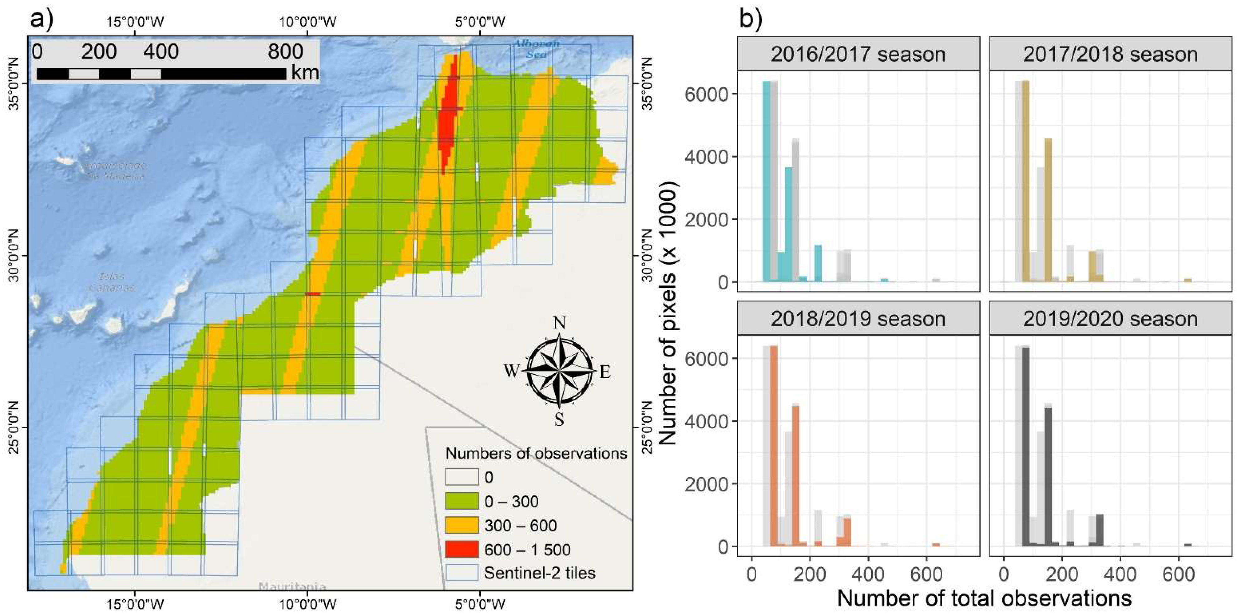
2.1. Study Area

In this study, the scale of research was country level, and the Kingdom of Morocco, spread over 710,850 km2, was chosen as our study area. The country is located in the north-western corner of the African continent between latitudes 21° and 36° N, and longitudes 1° and 17° W (Figure 1). Topographically, Morocco comprises a rugged mountainous interior, where the Atlas Mountains separate the northern part of the country from the wide desert areas in the south. Climatologically, the country has a wide variety of climates, ranging from the Mediterranean along the coasts, with mild winters and dry warm summers, to the continental in the interior, with colder winters and hot and dry summers. The southern part of the country as well as the east, contrary to the rest, are affected by the extreme dry climate of the Sahara Desert [38]. Morocco’s economy is largely dependent on agriculture, which accounts for about 15% of the country’s GDP as the first source of employment. The country produces many agricultural commodities. They include winter and spring crops (cereals and pulses) based in rainfed areas, and industrial crops (citrus, olive, sugar beets, sugarcane, cotton, and vegetable oils) located in irrigated areas and favorable rainfed zones. The main growing regions that can be used for crop production lie along the agricultural plains located between the Atlantic Ocean and the western side of the Atlas Mountains.

2.2. Software Tools and Processing Platforms

Because of the large study area, any type of remote sensing process was never going to be simple as it involves massively huge data volumes with highly variable compute and storage workloads (running into tera-to peta-bytes). This makes data processing highly difficult or impractical in regular systems. Therefore, a cloud computing platform for image processing is needed to handle efficiently the storage and exploitation of such large datasets. Google Earth Engine (GEE) has enabled us to overcome these constraints gradually by allowing petabyte- and planetary scale exploration and analysis of geospatial data. GEE provides public access to the most freely accessible satellite datasets, including the entire Landsat archives from 4 to 8, Sentinel missions, MODIS, and many other openly available weather and climate datasets, as well as digital elevation models. For the spatial and temporal manipulation of these datasets, GEE provides both JavaScript and Python application programming interfaces (API), which allow us to easily develop algorithms that work in parallel on the Google data computer facilities. Another open-source software tool that has been utilized in our work is the Collect Earth Online (CEO), which is a cost-effective tool that promotes consistency in locating, interpreting, and labeling reference data plots with high-resolution imagery (0.5 m, WorldView) for use in classifying and monitoring land cover/land-use change [39].

2.3. Methodology

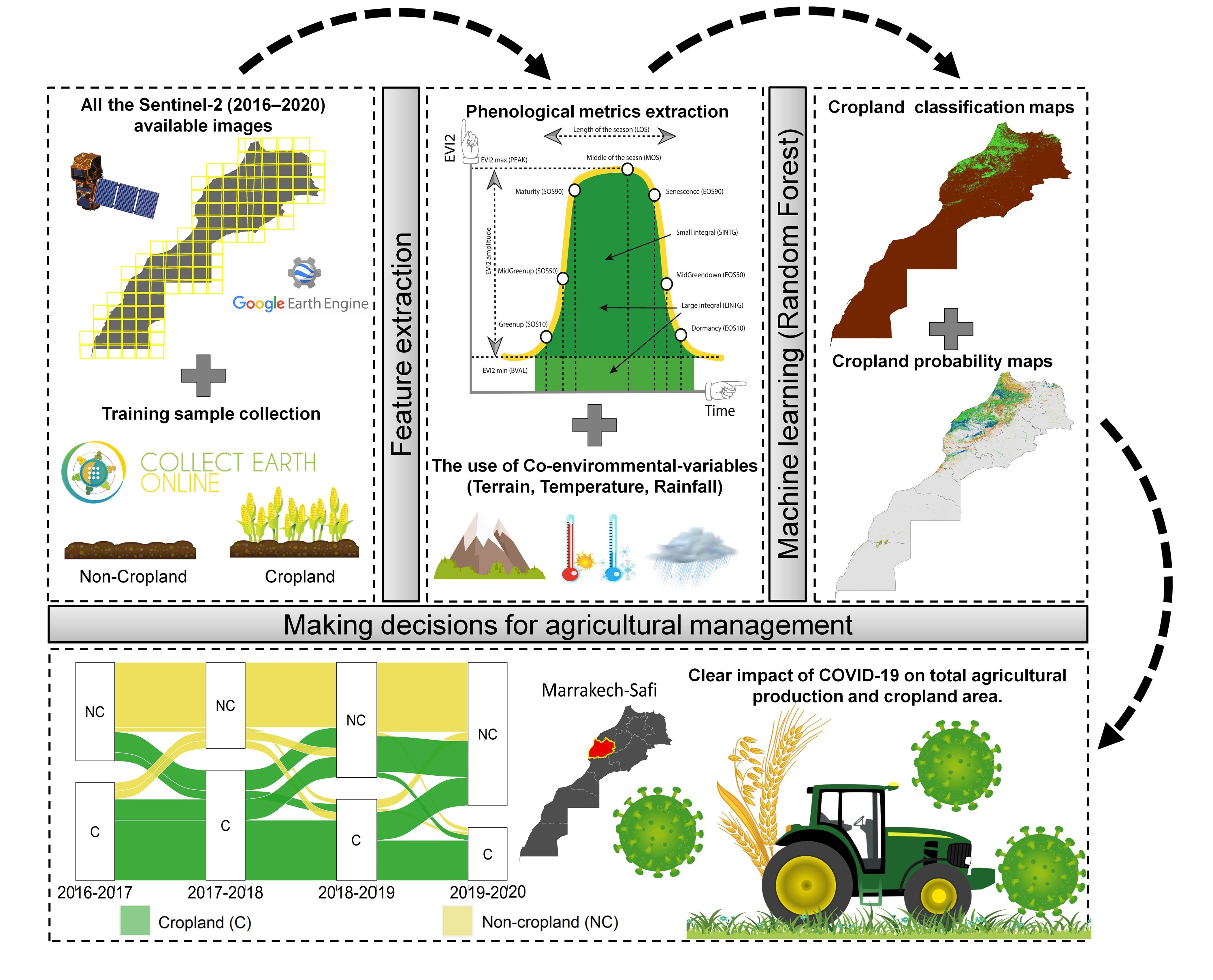
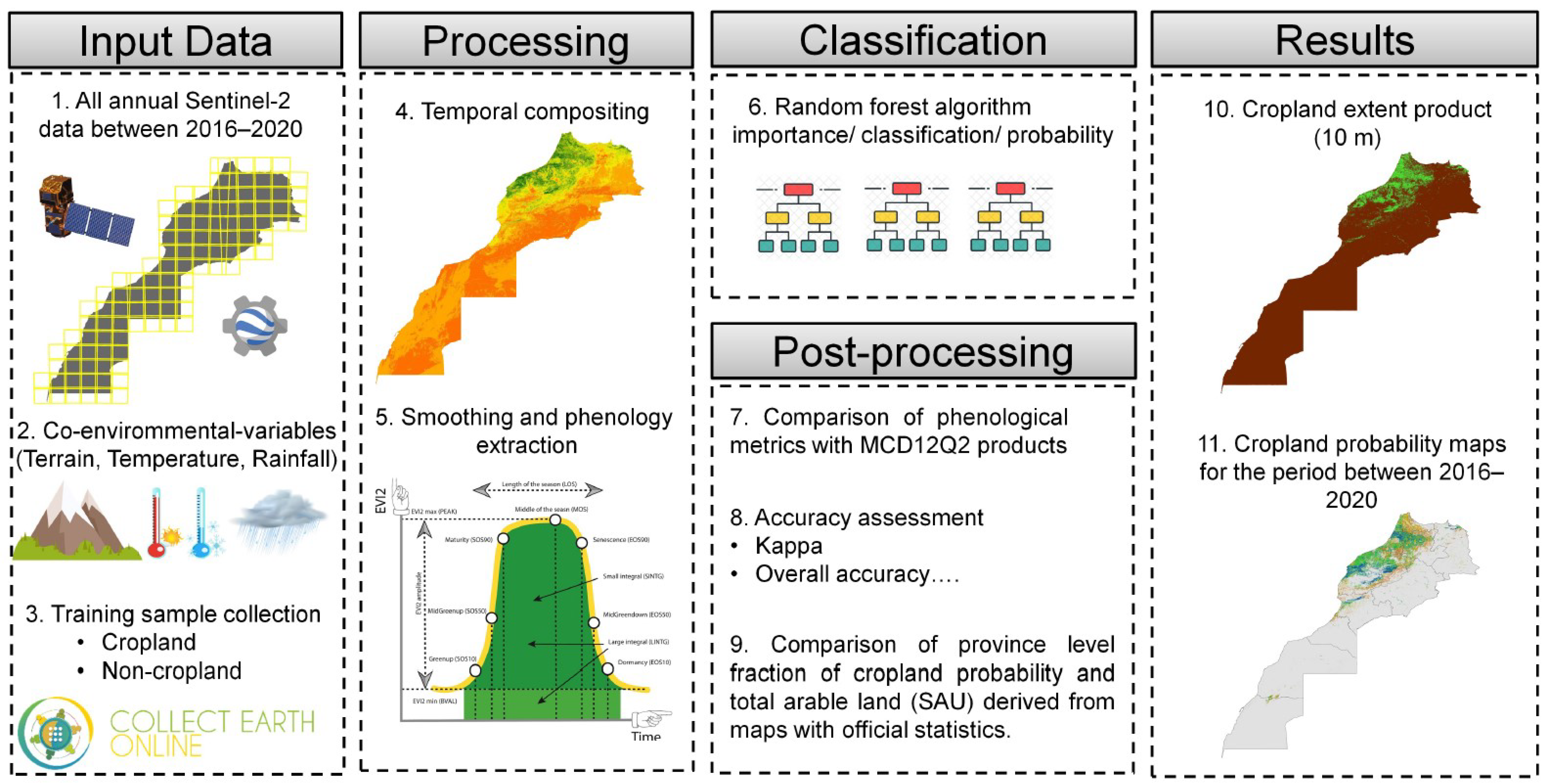
2.3.1. Workflow Description

Figure 2 shows an overview of the methodology followed in this research, outlining the steps (preprocessing, compositing, smoothing, phenological information extraction, classification, etc.) employed in mapping cropland extent based on the derived phenological information data.

2.3.2. Definition of Cropland Extent

It’s indispensable to any successful mapping to have a comprehensive and clear definition of what is being mapped. Thus, we adopted a cropland definition, which defines the croplands from a remote sensing perspective as “lands cultivated with plants harvested for food, feed, and fiber, including both annual crops as well as continuous plantations (e.g., coffee, tea, rubber, cocoa, oil palms) [40].

2.3.3. Data Preparation

Satellite Data

The primary datasets for this study came from the twin Sentinel-2A and Sentinel-2B satellites developed by the European Commission and the European Space Agency for global land observation within the Copernicus Program. Both satellites allow the availability of free multispectral imagery at high spatial resolution (10–60 m), with a revisiting cycle of up to 5 days. Two spectral bands were used in the current study: band 4 (665 nm) and band 8 (842 nm), with a spatial resolution of 10 m.
Overall, 56,258 Sentinel-2 scenes were acquired over the study area for the observation period from 2016 to 2020. This database was used to derive the cropland extent for a typical agricultural season that was regarded as starting on 1 September and ending on 31 August of the following year. Figure 3 illustrates the spatial distribution of the Sentinel-2 observations varies across Morocco from 2016 to 2020.
All Sentinel-2 images acquired using the GEE platform were Level-1C products (Top-Of-Atmosphere, TOA), meaning they were geometrically-corrected and radiometrically-calibrated, so they did not require any further preprocessing. These images, which have been atmospherically corrected (Level 2A), have also been included in GEE. However, for most parts of the study area in our present research, certain Level-2A assets prior to 2019 had not yet been processed and were held aside for future iterations.
Additionally, the EVI2 (two-band EVI, similar to the three-band EVI but blue band is not used) [41], was employed for detecting phenological features and capturing the change of vegetation cover in the period studied.
The two-band EVI was chosen in this study because, compared to the other more commonly used vegetation indices, it is less sensitive to soil background brightness and atmospheric scattering contamination and does not saturate over moderate-to-high densely-vegetated areas [41]. All these things explained why the EVI2 had the best performance in characterizing vegetation properties, estimating crop gross primary productivity and detecting more accurate phenological metrics than its traditional counterparts [42,43]. Thus, EVI2 has been successfully used to generate operational LSP products covering the entire globe and more comparable to in situ PhenoCam observations from both MODIS (MCD12Q2) and VIIRS data (VNP22Q2), which are the only global operational land surface phenology products currently available in the world for the scientific community [44,45,46].
It is computed as follows:
EVI 2 = 2.5 × ρ nir     ρ r ρ nir   + 2.4 ×   ρ r   + 1
where ρnir, and ρr stand for the atmospherically-corrected surface reflectance of the near-infrared and red (visible) bands.

Ancillary Features

Remote sensing-based land cover or vegetation classification accuracy can greatly benefit from including multiple types of ancillary data sources in a classification procedure. The term ancillary data refers to any data or information obtained from sources apart from remote sensing images [47], and which are used specifically in an interconnected way to support the process of image classification by increasing the separability between the classes. The ancillary spatial data used in this study is the slope of the topography extracted using a digital elevation model of the study area. Theoretically, it could point out regions of high elevation or steep slopes where cropland cover is not likely to exist.
In addition to this terrain feature, WorldClim V2 Bioclimatic variables [48] have been incorporated to account for the relationship between climatic conditions and cropland extent. These comprise 19 bioclimatic variables originally derived from long-term normal monthly climate data on temperature and rainfall collected from weather stations for the period of 1950–2000 and with a spatial resolution of 1 km2.
Lastly, two single layers of forest cover and water provided by GEE were employed to mask forest and water bodies and thus prevent class confusion and minimize processing time. Water surfaces, such as rivers and lakes, were masked out using the 30-m water body mask from [49], while forest was masked out using the Global PALSAR-2/PALSAR 30 m binary forest/non-forest map (JAXA FNF, Tokyo Japan) [50].
Before analysis, all auxiliary variables were reprojected and resampled to 10 m to match the spatial resolution of Sentinel-2 using the nearest neighbor interpolation in GEE platform.

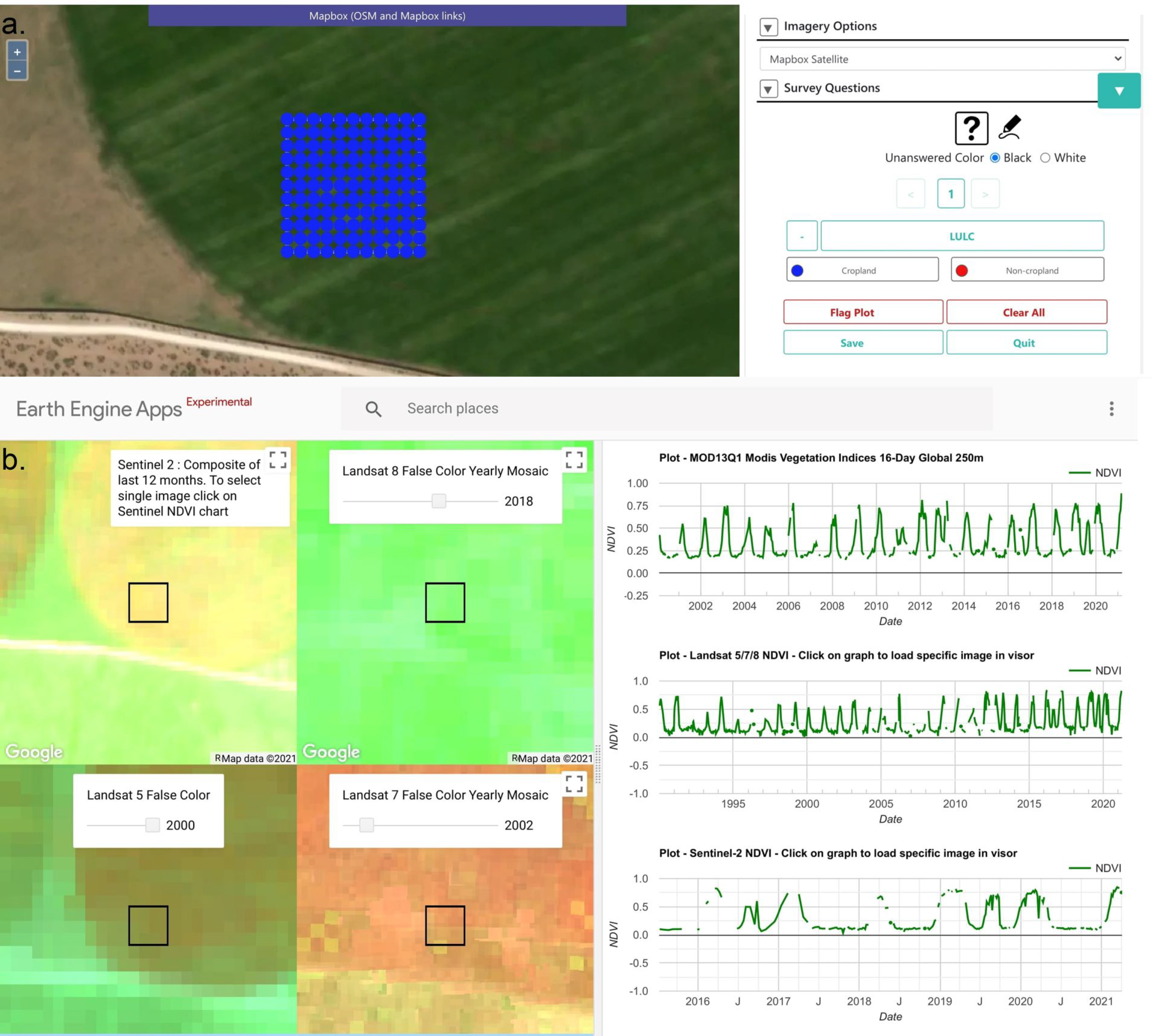
Collecting Training Data

Collecting cropland and non-cropland reference observations is often a complicated task because an agricultural activity is a constant phase that must be monitored over a long period of time. Satellite images with high spectral resolution have been a crucial option in this context. However, they are not sufficient to reconstruct the landscape’s historical dynamics. This study thus employs Collect Earth Online (CEO), whose full integration with Google Earth, Google Earth Engine, and other archives of freely accessible satellite imagery enables “augmented visual interpretation”, a process in which users assess very high spatial resolution imagery (0.5 m, World-View) in conjunction with geo-synchronized Landsat and Sentinel 2 images and a graphical user interface [39].
The reference data were therefore labelled according to observed land cover type using the CEO tool, where 1192 square-shaped sample plots were randomly distributed throughout the study area (Figure 1). In order to be as compatible as possible with the specific properties of Sentinel-2 data used in this analysis, each sample plot has a width of 100 m with sampling points positioned within at 10-m intervals for 121 points per plot (Figure 4).

2.3.4. Sentinel 10-Day Composite Images Construction

Temporal synthesis by image compositing with regular time intervals represents a valuable tool to overcome the spatial heterogeneity of observation images and generate consistent time series. The efficiency and simplicity of this technique make it extremely important for monitoring approaches targeting large areas, as it offers a range of advantages for data integration and analysis. Methodologically, there are a range of existing and established compositing approaches. To do so, an approach based on a general following of the best-pixel selection strategy was adopted, which picks the observation with the highest maximum observed value of the spectral index within a given regular temporal window that should be narrow enough to capture phenology information at field level. As a result, the calculated Sentinel-2 EVI2 data in this study was composited to construct a regular time series of EVI2 data at a 10-day interval for the period 2016–2020.

2.3.5. Smoothing and Phenological Metrics Extraction

A smoothing filter method is a necessary prerequisite step to reduce the noise of the involved input EVI2, which is most likely unrelated to real vegetation change or management practices [51,52]. Recalling the existence of several curve fitting methods, the Savitzky–Golay method (shortened to S-G) [53] was applied within the GEE platform as the filter function since it is able to denoise and attenuate the effect of cloudy and missing pixels particularly well compared to other well-known filters. The S-G method maintains and preserves the vegetation index profile by using a locally adaptive moving window that eliminates the outliers and corrects the errors present in the original time series [43]. The general Equation (2) of the filter is:
g i = n n C j f i + j      
where f i represents the original EVI2 value in the time series, g i is the filtered EVI2 value, and the weights are C j = 1 / 2 n + 1 , while the smoothing window size is 2n + 1, and wherein n is the half-width of the smoothing window.
The principle of this filter is to preserve high moments within the data [54]. Therefore, in Equation (3), the c n is not a constant, but a quadratic polynomial function that depends on the user’s preference and is used to fit each data value f i in the moving window:
c n t = c 1 + c 2   t + c 3   t 2
where t corresponds to the day of the year in the EVI2 time-series.
Selecting the appropriate size of the smoothing window and the degree of polynomial fitting is critical for the model’s ability to minimize the effect of outliers and simultaneously preserve the temporal detail in the EVI2 time-series. Hence, the half window size was set to 4, as suggested by Chen et al. [51] who have shown that this value is appropriate to better fit the time-series data. The result of the S-G smoothing method was a fitted EVI2 time series consisting of new values after noise removal, as shown in Figure 5.
Once the smoothed EVI2 time-series were generated, a phenology-retrieving technique should be used to extract key seasonality parameters in the study area. There are currently several approaches for retrieving phenology from time series of vegetation indexes [55].
In our study, we used the well-known dynamic threshold method, where the threshold is proportional to the seasonal amplitude of the vegetation index time series [33,56,57,58]. This technique is commonly used because it typically keeps dates within a certain reasonable range by assuming that a specific phenology, whether the start of season (SOS) or end of season (EOS), will start if the EVI2 ratio crosses a certain threshold during the EVI2 rising stage or decline stage, respectively. The EVI2 ratio ranges from 0 to 1 for each pixel and is defined as follows:
  EVI 2 ratio = EVI 2 t BVAL PEAK BVAL
where EVI 2 ratio is the EVI2 ratio; the EVI 2 t denotes the EVI2 at time t; while the PEAK and BVAL are the seasonal maximum and minimum EVI2 observations, respectively.
In this study, we used three thresholds (0.1, 0.5, and 0.9) corresponding to 10%, 50%, and 90% of the seasonal amplitude of EVI2 (AMPL= PEAK-BVAL) in spring and fall to extract SOS10, SOS50, SOS90, EOS10, EOS50, and EOS90 respectively (Figure 6).
In addition to these key phenophases, a variety of phenological metrics were extracted from the reconstructed satellite-derived EVI2 time series such as the small integral of the growing season (SINTG) which is effectively the sum of the integral functions fitted to each respective growing season occurring throughout a respective year, minus the area below the base level (this is a measure of the productivity within the growing season). In addition, it includes the large integral of the growing season (LINTG) which is the area under the curve of the fitting function from the start to the end of the growing period (an estimate of the total vegetation productivity in the annual cycle).
Our resultant metrics are shown graphically in Figure 6 and described in Table 1.

2.3.6. Comparison to MODIS Collection 6 MCD12Q2 Data

Based on our extracted vegetation phenology metrics, we performed a number of analyses to visually assess whether the resulting spatial patterns are smoother or whether there are any undesirable artifacts and patches, as well as comparing the resulted phenological metrics with the MODIS Collection 6 MCD12Q2 phenology product. As described before, those data are currently the only operational global land cover dynamics products that include the timing of vegetation phenology at global scales at a 500 m spatial resolution and annual time step.
In order not to inflate the number of explanatory pheno-variables, only three main metrics that relate well to biomass and seasonal timing productivity (Midgreenup, Midgreendown, and SINTG) were selected to be the basis for data validation in this study. Given that MCD12Q2 products were only available at yearly intervals from 2001 to 2018, we selected the season 2017–2018 to serve as the basis for phenology retrievals validation. The three Sentinel-2 derived phenological metrics for the same corresponding period were resampled to 500 m resolution to more closely fit MCD12Q2 spatial resolution for the purpose of statistically comparing our findings with MODIS’s phenological metrics. This aggregation was accomplished by taking the average Sentinel-2-derived phenological data of all 10 m resolution pixels for which the center is located within the geometry of a 500 m Modis grid cell. Furthermore, we assessed the relationship between resampled Sentinel-2 and MCD12Q2 metrics based on Pearson correlation coefficients (r) and the root mean squared error (RMSE).

2.3.7. Random Forest Machine Learning Algorithm

The classification algorithm employed for this research was the random forest (RF) technique, which is an ensemble learning method for classification (and regression) tasks that operates by constructing a large number of decision trees at the training phase and outputting the class that is the mode of the classes of the individual trees [59].
Owing to its higher accuracy, the RF algorithm has proven itself to be one of the more effective classifications approaches in several remote sensing applications, including cropland and crop type mapping, in which it achieves good results, as demonstrated by many recent papers [60,61].
Fortunately, the RF algorithm is included in the GEE platform, where, the function “ee.Classifier.smileRandomForest” was used to represent the classifier. The main RF‘s two tuning-parameters, mtry (number of different predictors tested at each node) and ntree (the number of trees) were set to the square root of available input variables (default) and to 250, respectively. Moreover, we calculated the variable importance of RF in GEE as a way to quantify the contribution that each feature variable has to improve the classification performance. The result of this classification is a map of cropland and non-cropland land cover for the nominal year 2019–2020 based on phenological features and environmental covariates of the same period.
The trained classification RF model for the 2019–2020 cropping season was run using the same input features for each remaining seasonal year in a probability mode instead of the classification mode option. In this last mode, RF applies majority voting to all trees for class prediction by default. However, in probability mode, the fraction of trees that vote for a certain class is calculated. This resulted in a yearly estimate of the probability (probability maps (0–100%)) of every pixel on whether it belongs to the cropland area or not.

2.3.8. Validation of the Cropland Extent Maps

The accuracy assessment in this study was based on cross-validation with repeated leave-p-out cross-validation method where 80% of the crop/non-crop samples (i.e., the training samples) were randomly assigned to training data and the remaining 20% were used as test data. The results were tabulated in a confusion matrix from which the widely applied overall accuracy (OA), producer’s accuracy (PA), and user’s accuracy (UA), Kappa coefficient, and the F1-score were computed and used to assess the quality of the derived cropland extent map [62].
In addition to the previous statistical accuracy assessment, and since the 10-m cropland classification and probability products are of high-spatial resolution, areas were calculated also at provincial units. We tried to perform a regression analysis for our derived areas and compared them with the area statistics available to us from the official agriculture statistics.
However, doing so is a challenge, because in many regions, including Morocco, agricultural statistics are outdated, of doubtful quality, or missing adequate sub-national historical inventory data. The only such data available is the Utilized Agricultural Land (Surface Agricole Utile—SAU), which is the sum of independent kinds of land which were really exploited in the growing season for agricultural and crop production.
To approach these statistics, and since they are available per province, it was decided to compute these areas by selecting only pixels that have a probability of more than 60% of being cropland to be classified as SAU areas, whilst all pixels having a probability of less than 60% of being cropland are classified as non-cropland class. The areas computed per province were compared with official statistics of provincially utilized agricultural land.

3. Results

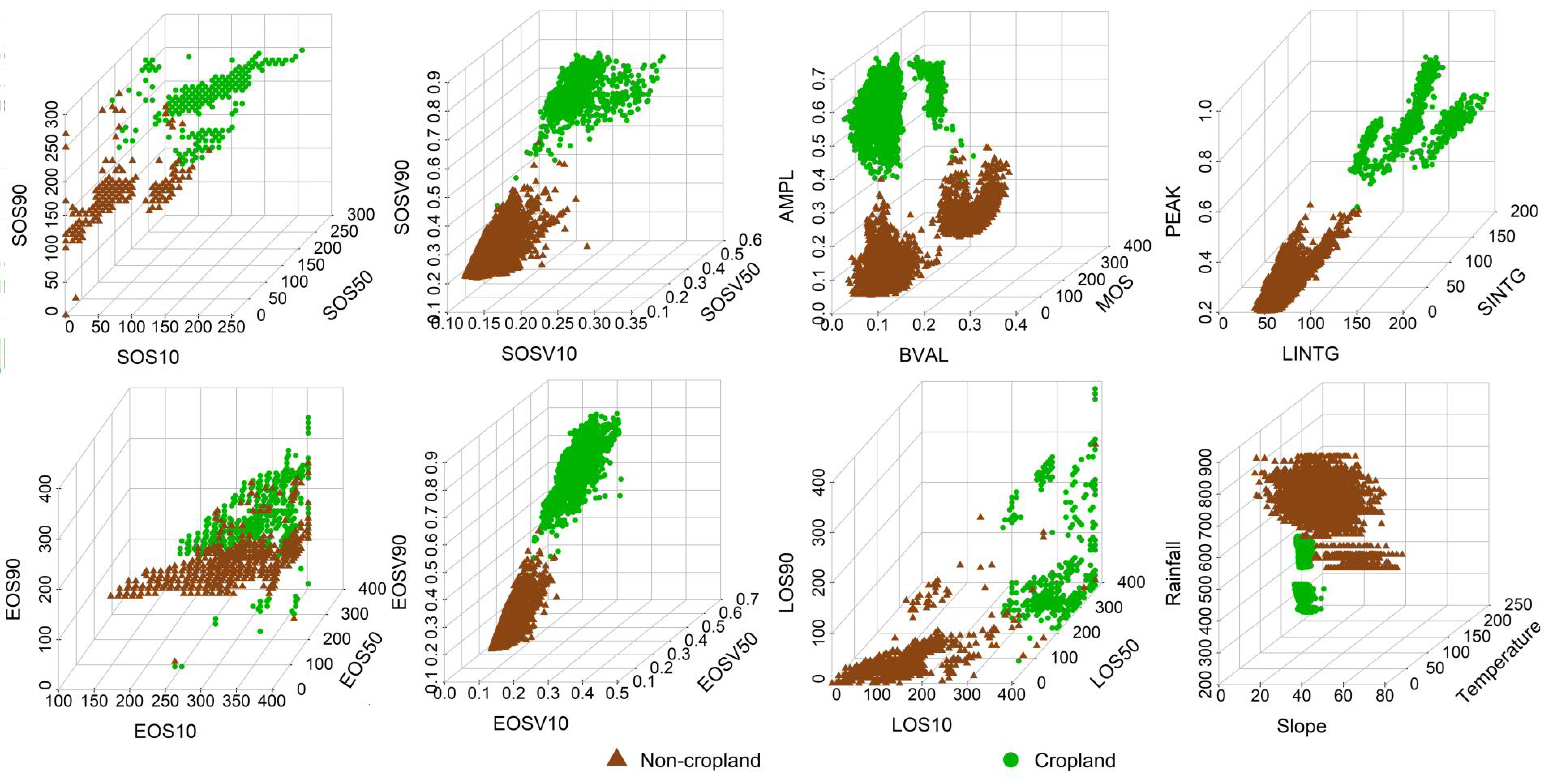
3.1. Verification of the Vegetation Phenology Results

Figure 7 shows national maps of three key phenological metrics (SOS50, EOS50, and SINTG) extracted by our GEE-based approach for the four years considered. The three phenological metrics derived appear to be generally spatially smooth and visually appealing. Moreover, their spatial patterns vary depending on the metric type and growing season’s properties. A point to consider is the patterns in the timing of midgreenup and midgreendown, as well as the integral of the EVI2 curve (Figure 7) show in general strong geographic variation related to climate forcing, land cover, and associated environmental variables.
It can be seen that the seasons 2016–2017, 2018–2019, and 2019–2020 have nearly the same yearly spatial pattern as Midgreenup (SOS50), whereas the year 2017–2018 was characterized by later SOS estimates in most parts of the country, with the exception of some irrigated areas in the central plains. Topographically, the timing of SOS50 values in higher elevation mountain areas were later (DOY > 200) than in lower elevation, flat areas with DOY ~100 (Figure 7). In addition to topography, this difference is most likely controlled by climatic conditions (temperature and precipitation), as can be deduced from the grey areas where no SOS data is detected; those areas are either too cold and frequently frozen to support sufficient crop growth (high elevations) or too dry to accommodate crop production without irrigation (the desert regions in the south and east of the country).
Geographic variation in mid-green-down timing (EOS50) is similar to SOS50 estimates, with the same relationship to climate forcing and associated environmental variables geographically and temporally across the studied years. It is clear that most areas exhibit a later EOS, with the exception of irrigated areas in the central plains and dense forest in the mountains, where a tendency for an earlier SOS and later EOS are shown. Similar to SOS, EOS dates can still not be estimated in the southern part of the country because the EOS dates in these regions were recorded prior to BVAL being selected for both EOS and SOS estimates in this study.
The annual national-scale patterns in SINTG reflect geographic patterns in vegetation productivity, across the country (Figure 7). For example, EVI2 SINTG associated with irrigated areas in the north and east part is clearly evident. In contrast, and as expected, EVI2 SINTG represents low to no vegetation productivity, and was measured in the mountainous regions and in the desert areas of the country in the south and east, although localized patches of high EVI2 SINTG associated with the presence of oasis in these latter regions are clearly evident as well.
Figure 8 presents a fine-scale spatial comparison of the selected sites in Figure 7 and between the three Sentinel-2 phenological metrics for the 2017–2018 agricultural season.
As expected, the 10 m spatial resolution of Sentinel-2 phenological images has allowed it faithfully to capture more detailed spatial distributions of phenology (Figure 8). In comparison to Figure 7, the detailed view of the GEE-based approach and Sentinel-2 results clearly illustrate the amount of field-to-field variation, enabling crop phenology retrievals to be measured and assessed at the field and finer scales over very large areas. It’s worth mentioning that each field is likely to exhibit a different phenological status due to different field conditions, farmer’s practices, and the particular crop type cultivated.
To illustrate statistically the character and quality of phenology metrics provided by our approach, Figure 9 shows a statistical summary that compares our results with the MCD12Q2 retrievals for SOS50, EOS50 dates, and SINTG curve area based on a random sample of pixels over every one of the two sets selected across the study area.
Overall, inter-observer correspondence was excellent for measurements between our results versus MCD12Q2 within the SOS, the EOS, and the SINTG (r = 0.81, r = 0.89, r = 0.79, respectively), which indicates a comparable phenology retrieval and a relatively consistent temporal pattern. The RMSE results confirm that Sentinel-2 correctly matched the observations derived from MCD12Q1, with the generally smallest errors for EOS and SINTG (RMSE = 10 days, RMSE = 4.60, respectively). However, the RMSE value of SOS estimates was slightly larger compared to EOS (RMSE = 15 days).

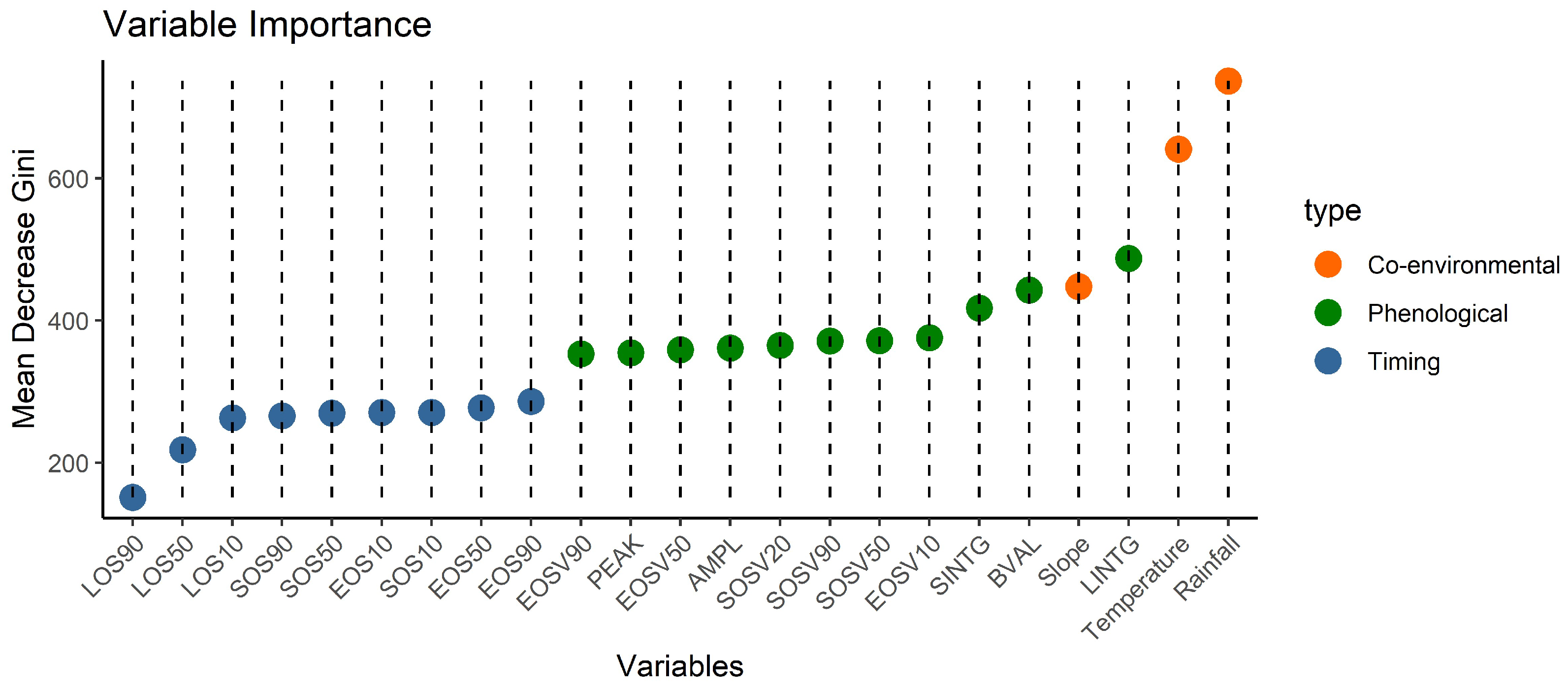
3.2. Phenological Feature Importance

In order to assess the power of phenological and environmental covariates to distinguish between cropped and non-cropped lands, we used a 3D approach to provide a descriptive analysis between the cropland classes and phenological features by looking at the shape of the pixel distribution in Figure 10. The figure shows a series of three-dimensional scatter diagrams of the two classes of cropland and non-cropland created using all the phenological and co-environmental variables integrated into the classification process.
In general, both classes appear to be well segregated and separable in the data space of all features. Consequently, all variables are able to separate croplands from non-croplands. In particular, the productivity metrics such as LINTG, SINTG, AMPL, PEAK, BVAL, and EVI2 value metrics (e.g., SOSV and EOSV) as well as the environmental covariates that configure good separability between the two classes. On the other hand, only a very small part of one particular class may be misclassified as the other class due to the existence of similar characteristics in timing metrics (e.g., SOS, EOS, and LOS) that show less power discrimination among other features.
These assumptions can be supported by results obtained through one of the strengths of RF models when compared to the more traditional supervised classification techniques, which is the ability to measure and assess the contribution of each predictor variable used within the classification (Figure 11). The variables’ importance was calculated based on the mean decrease in the Gini index.
According to this index, the environmental covariates (rainfall and temperature) were identified as being of utmost relevance for discriminating between cropland and non-cropland, closely followed by other productivity and EVI2 value metrics (i.e., LINTG, BVAL, SINTG, and vegetation index values at particular times; Figure 11). Another predictor that seemed to be playing a major role in the classification model as shown in Figure 11 was the slope as a topographical separator of cropland in its distribution. The contribution of timing metrics (i.e., SOS, EOS, and LOS) was again less strong than the contribution of the productivity metrics, as already described in Figure 10.

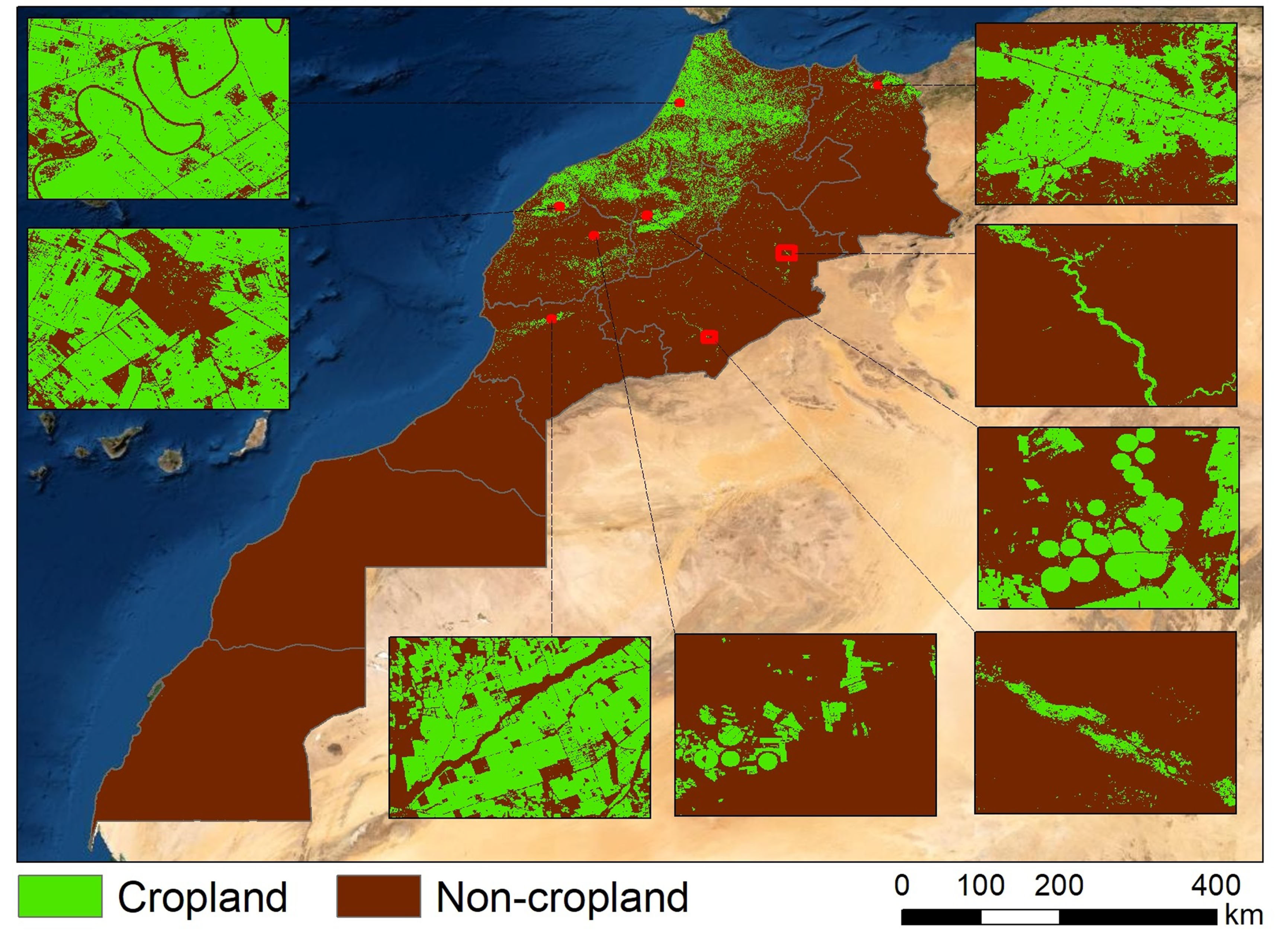
3.3. Cropland Extent Map and Accuracy Assessment

Based on the phenological and co-environmental features derived from GEE, a supervised classification for the nominal year of 2019–2020 was implemented using the RF trained model to separate croplands versus non-croplands as mentioned in Section 2.3.7 and assessed in Section 2.3.8. Figure 12 presents the 10 m country’s cropland map extent generated for the nominal 2019–2020 agricultural season using all the phenological and environmental covariate features. The cropland area is displayed in totality, with highlighted zoom-in views for some selected locations to show details.
A visual inspection of the national-scale cropland map depicts the typical patterns of the country’s cropland, where regional differences in cropping practices can be easily observed across the territory. The cropland seems to be concentrated near the coast and in the uplands, where precipitation is higher. However, some oasis-based cereal production and date harvesting can be identified just in the middle of the desert where precipitation is scarce. The eight zooms provided show croplands in great detail at a fine spatial resolution (1 pixel = 0.01 ha) over different landscapes, ranging from intensive large fields in the western part of the country to fields under pivot irrigation in the central plains and oasis areas in the desert that often surround a water source. Table 2 reports the classification accuracy values and the confusion matrix derived from the analysis of the validation dataset.
The overall accuracy of the cropland classification was found to be 97.86% with a Kappa coefficient of 0.95 (Table 2). According to these findings, it is clear that using phenological metrics in conjunction with topographic and climatic variables can help with cropland type identification.

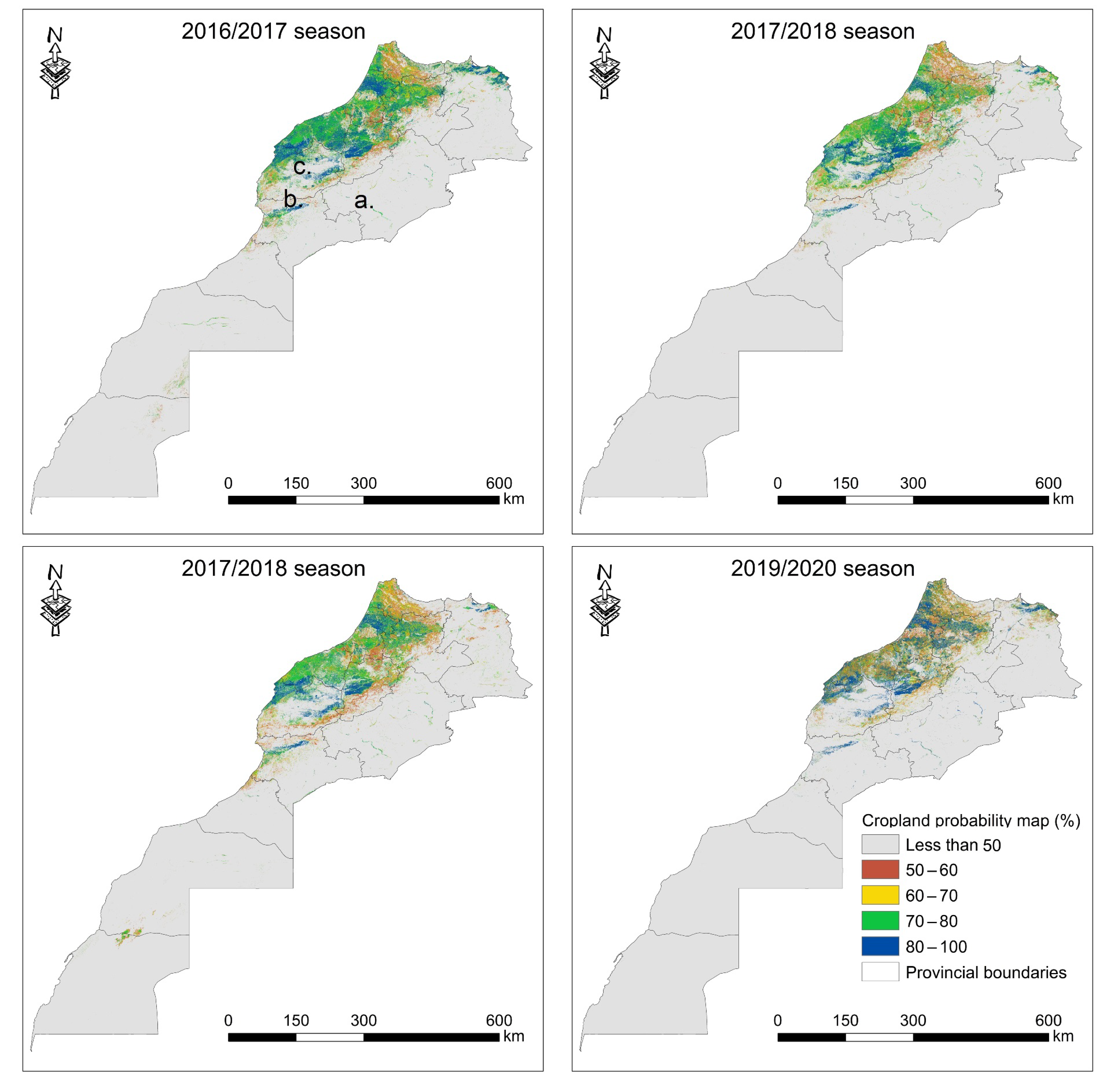
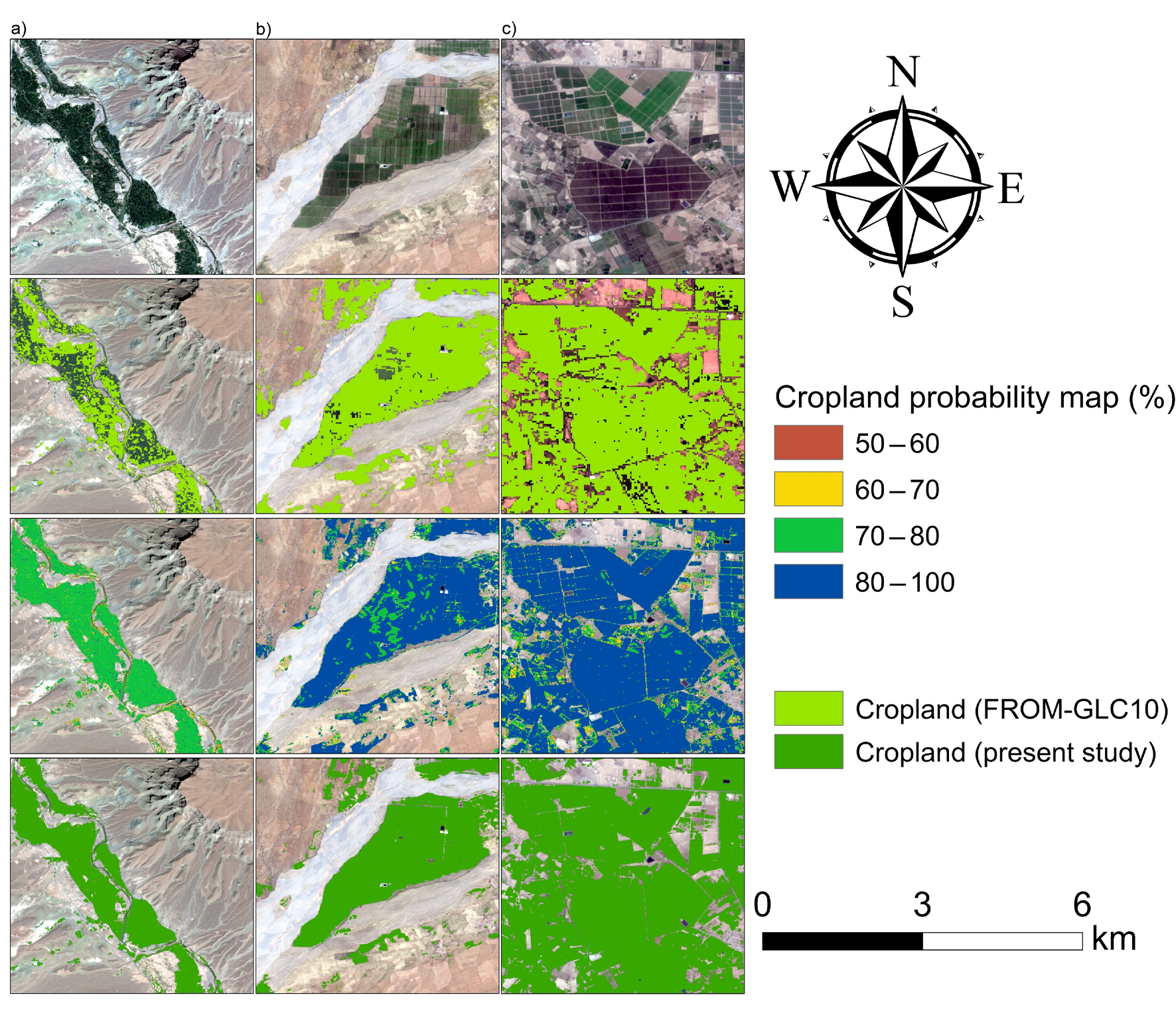
3.4. Probability-Based Cropland Maps

When classifying images using random forest classification, probability maps can be computed and generated as well. In order to do that, we apply the RF-based classifiers trained in the 2019–2020 agricultural season to the other seasons using the same derived features. As previously described, we chose the “probability” mode for GEE’s RF algorithm this time. The output is the probability that the classification is correct so that the results can be evaluated, filtered, and refined to improve the algorithm’s detection capabilities. Figure 13 shows the probability of each pixel belonging to a cropland class over the four studied seasons.
Similar to classification results, it is notable that the north-eastern corner of Morocco has the highest probability of cropland compared to the western and southern parts. Figure 14 shows a detailed view of the three selected sites highlighted in Figure 13 for the season of 2016–2017. Our produced probability and cropland maps in these areas were compared and are shown alongside very high-resolution images and the 2017 10-m FROM-GLC10 products with 10 land cover types, including the cropland classes (Figure 14).
In the three study areas, it can be seen that the proposed approach was able to successfully identify the cropland distribution corresponding to areas with a high probability (60%<) whereas non-cropland areas exhibit a low probability of being classified as cropland. This happened to be consistent with the reference image, with nearly no salt–pepper effect or noise that significantly affected the inaccuracy of the mapping.

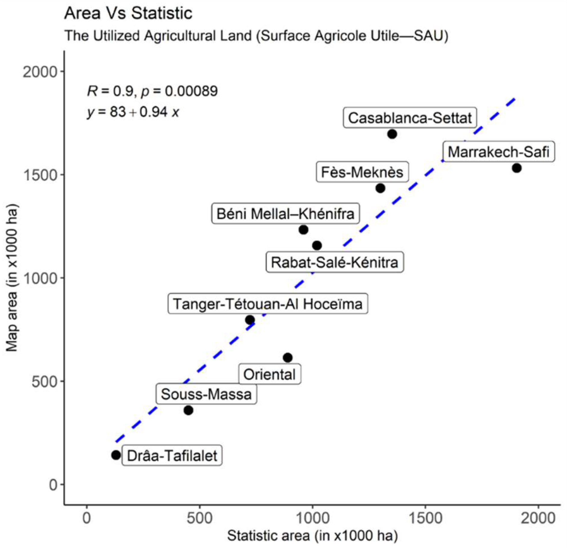
3.5. Comparison with National Statistics

Apart from producing a map, the calculation of cropland area statistics is an important resource for local governments when they seek to monitor cropland changes. For that reason, a validation exercise, which reveals the overall error structure of the derived cropland areas must be considered. However, we must mention that one of the limitations of such things has been the lack of updated statistics on cropped areas on a national scale, especially in Morocco. The only such data available is the total arable land or utilized agricultural land (Surface Agricole Utile—SAU). To approach these statistics, a selected threshold value of 60% (“probability filter”) was used to reclassify the probability maps into categorical maps distinguishing between SAU and non-SAU areas. Figure 15 compares the maximum province-level SAU proportions (%) from our results during the studied period with the reported statistics of the provincial utilized agricultural land.
The results show that our approach provides an accurate areal estimate of cultivated SAU areas across Morocco at both national and regional scales regarding the linear regression that revealed a high correlation of r = 0.9 with most provinces falling reasonably close to the 1:1 line (Figure 15). However, differences were observed in some regions, in which our classification identifies fewer SAU and cropland areas compared to official statistics.

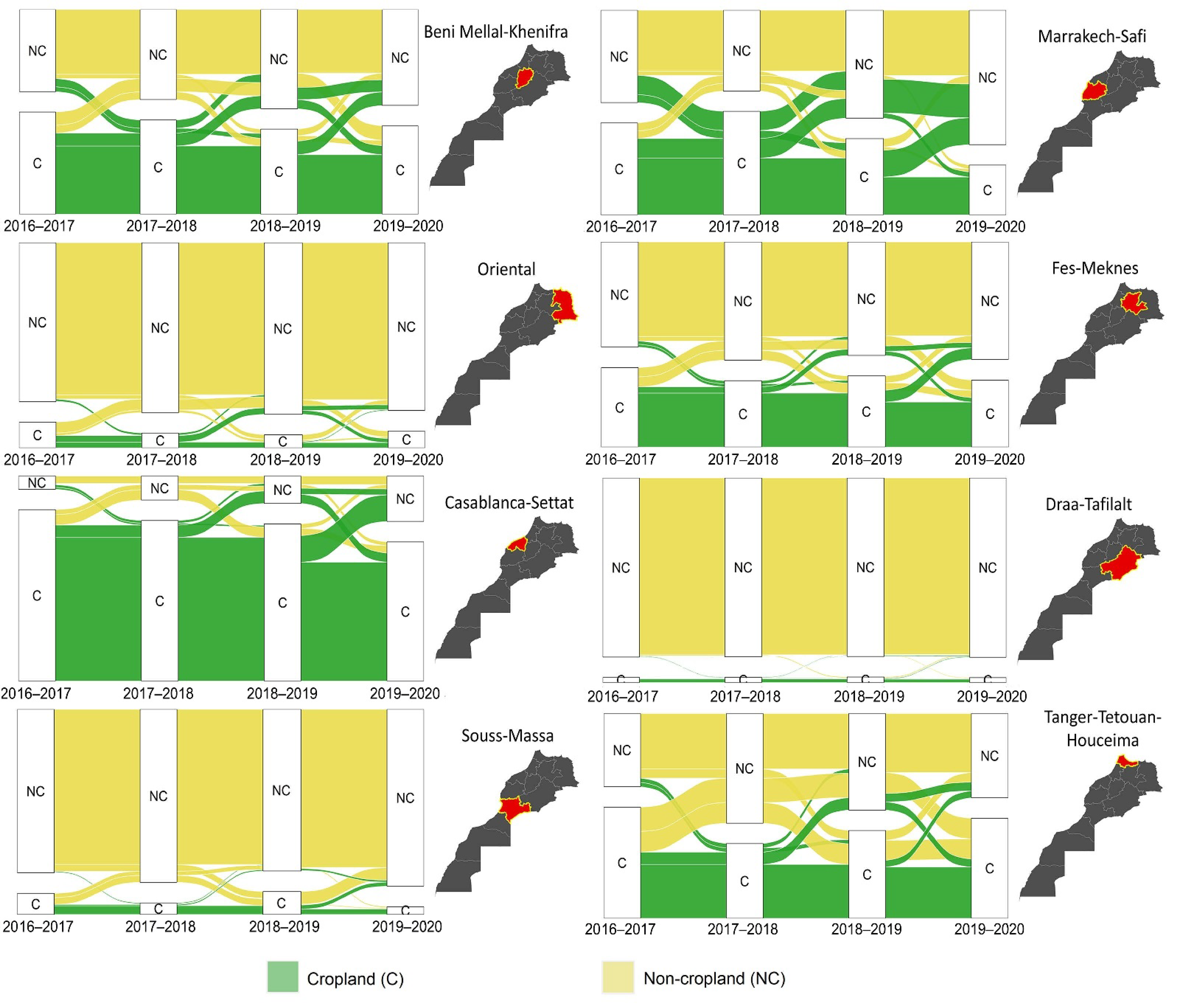
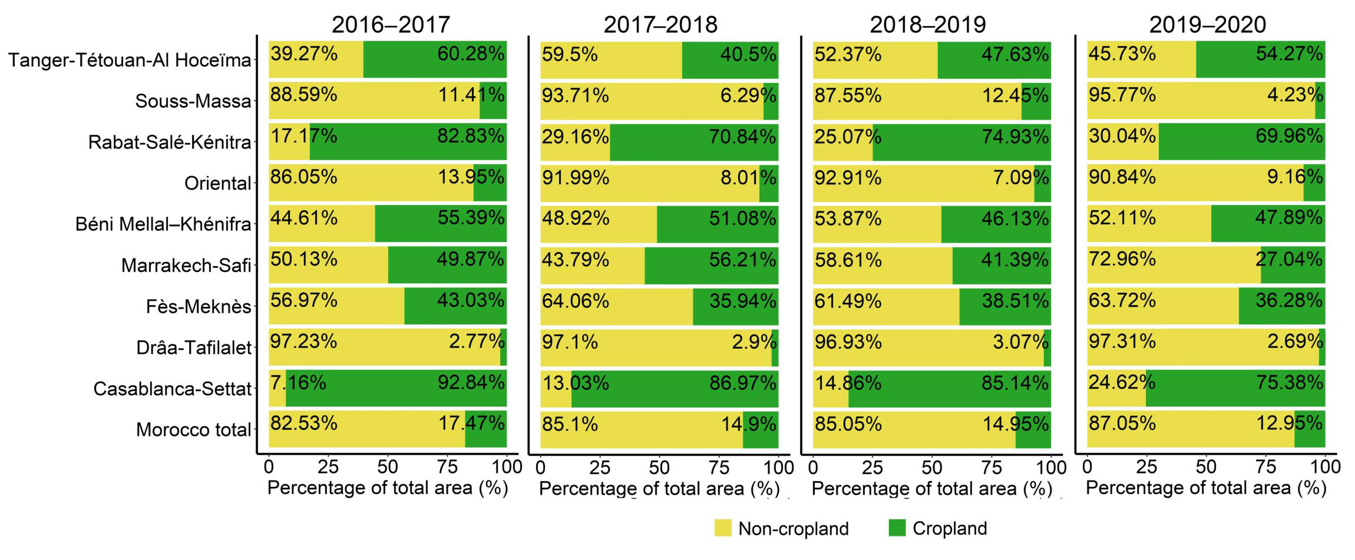
3.6. Cropland Dynamics in the Area

The Sankey diagram (Figure 16) depicts the fluxes of cropland and non-cropland classes derived from the probability maps with a 60% threshold filter to visualize from-to cropland change transitions in the area of Morocco between 2016 and 2020. Each column of colored nodes represents a seasonal year and each node within the columns represents a land cover type. The height of a node is proportional to the area of that particular land cover type for a given year. The transitions of a proportion of the landscape from one class type to another are represented by colored lines of differing thickness linking nodes, so that one can trace back from 2016 to 2020 to assess how areas have been changed.
This graph effectively summarizes the percentage of cropland areas with the highest probability in each region over the four years studied. As depicted in the figure, a permanent flow (i.e., pixels assigned to a given class in one year remaining the same in the next year) towards cropland areas in 2019–2020 per all the region originated from its own class from 2016 to 2018. This means that they do not indicate transitions, but their maintenance over time. However, when the flows from the same class are discarded, the cropland areas with the highest probability have experienced a great absolute change in surface area between 2016 and 2019 in all regions except Draa-tafilalet, where a small amount of net change is found.
We can see a significant decrease in cropland areas in 2019–2020 that is noticed to be largely converted to non-cropland areas (thicker lines) compared to the trend of change for the rest of the years. This flow is not unique to a region but is being repeated in all the other regions, specifically in Marrakech Safi and Casblanca-Settat, where this area has decreased by approximately half since 2016–2017, which implies a higher cropland cover loss in these regions. Another flow that occurs in cropland transitions is that certain areas mapped as cropland in 2016–2017 transitioned to non-cropland class the following season and then half of these returned to cropland, with the other half remaining non-cropland in 2018–2019.

4. Discussion

For sustainable agriculture production and food security, having up-to-date national-scale cropland maps that are detailed, accurate, and at high spatial resolution is more than critical [40]). This study examined the potential of a phenology-based algorithm to map and identify cropland areas within GEE and at high spatial resolution. In this context, the GEE cloud platform was found to be a valid tool and processing environment to produce a precise and accurate cropland extent product, and all its computational power and well-integrated analysis techniques on a large scale were done in a matter of minutes, as has been reported by other authors [63].
Among the resource satellites currently available, Sentinel-2 was chosen as a base to classify and map cropland distribution at the field scale due to its exceptional revisit frequency of 5 days (twin satellites S2A and S2B) and its spatial resolution of 10 m per pixel. Sentinel-2 is, therefore, more adequate to the diversity of the agro-ecological context, landscape patterns, and agricultural practices present in Morocco and such regions, where fields and farms are on average 0.9 hectares in size and only such high spatial resolution data can provide enough information for efficient and detailed crop monitoring and classification.
Our approach is based essentially on the use of extracted phenological characteristics (metrics) for cropland type mapping as they have already proved their efficacy and usefulness for monitoring and discriminating different vegetation cover over different scales [64].
Our findings show that cropland phenology data can be reliably detected in GEE using high temporal and spatial resolution satellite imagery. The SOS, EOS, and SINTG estimates using GEE’s Sentinel-2 data were strongly correlated with corresponding estimates from combined MCD12Q2 products (r > 0.80). This finding was also reported by Descals et al. [58], who found very good agreement between SOS and EOS estimates of Sentinel-2 and MODIS metrics in the arctic regions.
Interesting to note as well, is that most phenological retrieval software or products focus on major phenological metrics only, while our approach has no such limitation and can extract more than 20 metrics from the phenological profile. This wealth of phenological data is devoted to ensuring the greatest degree of separability between croplands and various types of land-cover types, as shown in Figure 10. Moreover, the use of ancillary data such as slope, temperature, and rainfall information were effective in improving classification and the quality of results that seem to be consistent with other research that found that these environmental covariates helped class separability significantly. By using all phenological metrics coupled with ancillary data, we were able to map the cropland distribution within the nominal year of 2019–2020 with an accuracy of 97.86% using the RF classifier. These findings clearly imply a high degree of confidence in identifying croplands versus non-croplands across large areas such as Morocco, which supports evidence from previous observations such as the GFSAD30AFCE dataset achieved relatively higher mapping accuracy in Africa because it took into consideration phenological information [19].
The results also proved the robustness of RF implemented in GEE to obtain accurate cropland extent over a very large area. The RF classifier was chosen because it needs few parameters to tune, gives more accurate results than most of the state-of-the-art methods, is computationally efficient in handling large-scale data, and generates a probability for each label [60,65]. This last benefit acts to provide a soft classification (probability estimation), which is particularly helpful in Africa’s fragmented and complex landscapes because hard classification will have higher uncertainties that arise when multiple classes occupy the same pixel at the same time [37,66]. The resulting probability maps captured by our approach correspond well with high resolution images (Figure 14). The probability maps were converted into “hard” results, considering a 60% probability threshold, in relation to which a given pixel was assigned to the cropland or non-cropland classes. Such results proven to be a significant improvement compared to existing products as shown in the same figure, this superiority lies in the incorporation of phenological data in our proposed framework, which serve as an important and powerful asset to map cropland and its change compared to traditional image stacking approach that could misses important phenological events thus makes cropland or crop type much difficult. Another shortcoming of existing products is their emphasis on LULC, where detailed mapping of croplands is not always the primary goal. Aside from that, they are only available for certain years and are not updated regularly [67].
The produced results were used to calculate the cropland areas of Morocco at the sub-national level for nine provinces and compare them with the total arable land (SAU) areas as shown in Figure 15. The relationship between province wise areas from both sources shows a very high correlation with an r value of 0.9, which demonstrated the ability of our approach to compute efficiently sub-national province level cropland area statistics and SAU.
Figure 16 and Figure 17 depict cropland distribution and dynamics over Morocco between 2016 and 2020. The remote sensing analysis shows a dramatic change in cropland areas that decreased significantly in the season of 2019–2020 compared to the remaining years in almost all the provinces. In particular, the areas of cropland decreased in Morocco by almost 5%, as they fell by 35,550 km2 from 2016 to 2020 (Figure 17).
It has to be noted that these significant decreases could be due to climate conditions. These assumptions are backed by the particularity of agriculture in Morocco, which depends strongly on rainfall distribution [68]. However, other factors accounted for the dramatic magnitude of change, such as the coronavirus disease 2019 (COVID-19), which not only has far-reaching effects on human health, but also economic impacts around the world, with all countries adopting unprecedented measures such as home confinement, travel bans, and business closures to control the rate of infection, but with major repercussions on labor markets and economic growth, and most importantly, the daily movement of farmers to their lands [69,70]. This assumption comes as no surprise since the most provinces with significant decrease, Casablanca-Settat, and Marrakech-Safi regions, have been in fact reporting the highest number of COVID-19 cases from the start of the pandemic to April 2020 in all of Morocco [71].

5. Conclusions

The study generated a yearly cropland distribution at a 10-m resolution over very large fragmented and complex areas (e.g., Morocco) using multi-year (2016–2020) phenological information, random forest machine learning algorithms, a large volume of reference training, and validation datasets from multiple sources by utilizing the big-data management and processing power of the Google Earth Engine cloud-computing platform. These methods and approaches demonstrated the ability to map croplands and their probabilities at a large big-country scale using petabyte volumes of big data. The resulting 10-m derived cropland extent products for the nominal season 2019–2020 had overall accuracies of over 97%. For the remaining years, a method for crop probabilities estimation was developed and evaluated based on the trained random forest model. The results maps compare well with province-level cropland statistics. This study paves the way to provide a high-resolution cropland extent map for countries where detailed spatial information of croplands is scarce as well as for more large-scale cropland extent mapping for more detailed products such as crop intensity, crop type, and crop irrigation. Additionally, annual cropland maps could be updated on a regular basis using this automated method in order to monitor cultivated area extension and abandonment over very large areas.

Author Contributions

Conceptualization, A.H., A.B. and T.B.; methodology, A.H.; software, A.H.; validation, A.H., A.B. and T.B.; formal analysis, A.H.; resources, A.H., A.B. and A.C.; data curation, A.H.; writing—original draft preparation, A.H.; writing—review and editing, A.B., A.C. and T.B.; visualization, A.H.; supervision, A.B. and T.B. All authors have read and agreed to the published version of the manuscript.

Funding

This research received no external funding.

Institutional Review Board Statement

Not applicable.

Informed Consent Statement

Not applicable.

Data Availability Statement

The Google Earth Engine (https://earthengine.google.com/ (accessed on 15 October 2020)) is a free and open platform that combines a multi-petabyte catalog of satellite imagery and geospatial datasets with planetary-scale analysis capabilities. The models and codes generated from this study are available upon request to the corresponding author.

Acknowledgments

The authors would like to thank the Google Earth Engine team for providing cloud-computing resources and European Space Agency (ESA) for valuable open-access Sentinel data. In addition, the authors would like to thank FAO and NASA for providing access to Collect Earth Online platform. The authors would also like to thank the anonymous reviewers for their very competent comments and helpful suggestions. The authors acknowledge the financial support of the National Centre for Scientific and Technical Research (CNRST) under the Excellence Research Scholarships Program.

Conflicts of Interest

The authors declare that they have no known conflicts of interest or personal relationships that could have appeared to influence the work reported in this paper.

References

  1. Kadam, N.N.; Xiao, G.; Melgar, R.J.; Bahuguna, R.N.; Quinones, C.; Tamilselvan, A.; Prasad, P.V.V.; Jagadish, K.S. Agronomic and Physiological Responses to High Temperature, Drought, and Elevated CO2 Interactions in Cereals. Adv. Agron. 2014, 127, 111–156. [Google Scholar] [CrossRef]
  2. Thenkabail, P.S.; Wu, Z. An Automated Cropland Classification Algorithm (ACCA) for Tajikistan by Combining Landsat, MODIS, and Secondary Data. Remote Sens. 2012, 4, 2890–2918. [Google Scholar] [CrossRef] [Green Version]
  3. Delrue, J.; Bydekerke, L.; Eerens, H.; Gilliams, S.; Piccard, I.; Swinnen, E. Crop Mapping in Countries with Small-Scale Farming: A Case Study for West Shewa, Ethiopia. Int. J. Remote Sens. 2013, 34, 2566–2582. [Google Scholar] [CrossRef]
  4. Waldner, F.; Fritz, S.; Di Gregorio, A.; Plotnikov, D.; Bartalev, S.; Kussul, N.; Gong, P.; Thenkabail, P.; Hazeu, G.; Klein, I. A Unified Cropland Layer at 250 m for Global Agriculture Monitoring. Data 2016, 1, 3. [Google Scholar] [CrossRef] [Green Version]
  5. Bartholome, E.; Belward, A.S. GLC2000: A New Approach to Global Land Cover Mapping from Earth Observation Data. Int. J. Remote Sens. 2005, 26, 1959–1977. [Google Scholar] [CrossRef]
  6. Arino, O.; Gross, D.; Ranera, F.; Leroy, M.; Bicheron, P.; Brockman, C.; Defourny, P.; Vancutsem, C.; Achard, F.; Durieux, L. GlobCover: ESA Service for Global Land Cover from MERIS. In Proceedings of the 2007 IEEE International Geoscience and Remote Sensing Symposium, Barcelona, Spain, 23–27 July 2007; IEEE: Barcelona, Spain; pp. 2412–2415. [Google Scholar]
  7. Latham, J.; Cumani, R.; Rosati, I.; Bloise, M. Global Land Cover Share (GLC-SHARE) Database Beta-Release Version 1.0-2014; FAO: Rome, Italy, 2014. [Google Scholar]
  8. Friedl, M.A.; McIver, D.K.; Hodges, J.C.F.; Zhang, X.Y.; Muchoney, D.; Strahler, A.H.; Woodcock, C.E.; Gopal, S.; Schneider, A.; Cooper, A.; et al. Global Land Cover Mapping from MODIS: Algorithms and Early Results. Remote Sens. Environ. 2002, 83, 287–302. [Google Scholar] [CrossRef]
  9. Pan, L.; Xia, H.; Yang, J.; Niu, W.; Wang, R.; Song, H.; Guo, Y.; Qin, Y. Mapping Cropping Intensity in Huaihe Basin Using Phenology Algorithm, All Sentinel-2 and Landsat Images in Google Earth Engine. Int. J. Appl. Earth Obs. Geoinf. 2021, 102, 102376. [Google Scholar] [CrossRef]
  10. Herold, M.; Mayaux, P.; Woodcock, C.E.; Baccini, A.; Schmullius, C. Some Challenges in Global Land Cover Mapping: An Assessment of Agreement and Accuracy in Existing 1 Km Datasets. Remote Sens. Environ. 2008, 112, 2538–2556. [Google Scholar] [CrossRef]
  11. See, L.; Fritz, S.; You, L.; Ramankutty, N.; Herrero, M.; Justice, C.; Becker-Reshef, I.; Thornton, P.; Erb, K.; Gong, P. Improved Global Cropland Data as an Essential Ingredient for Food Security. Glob. Food Secur. 2015, 4, 37–45. [Google Scholar] [CrossRef]
  12. Htitiou, A.; Boudhar, A.; Benabdelouahab, T. Deep Learning-Based Spatiotemporal Fusion Approach for Producing High-Resolution NDVI Time-Series Datasets. Can. J. Remote Sens. 2021, 47, 182–197. [Google Scholar] [CrossRef]
  13. Nguyen, M.D.; Baez-Villanueva, O.M.; Bui, D.D.; Nguyen, P.T.; Ribbe, L. Harmonization of Landsat and Sentinel 2 for Crop Monitoring in Drought Prone Areas: Case Studies of Ninh Thuan (Vietnam) and Bekaa (Lebanon). Remote Sens. 2020, 12, 281. [Google Scholar] [CrossRef] [Green Version]
  14. Htitiou, A.; Boudhar, A.; Lebrini, Y.; Lionboui, H.; Chehbouni, A.; Benabdelouahab, T. Classification and Status Monitoring of Agricultural Crops in Central Morocco: A Synergistic Combination of OBIA Approach and Fused Landsat-Sentinel-2 Data. J. Appl. Remote Sens. 2021, 15, 014504. [Google Scholar] [CrossRef]
  15. Azzari, G.; Lobell, D.B. Landsat-Based Classification in the Cloud: An Opportunity for a Paradigm Shift in Land Cover Monitoring. Remote Sens. Environ. 2017, 202, 64–74. [Google Scholar] [CrossRef]
  16. Gorelick, N.; Hancher, M.; Dixon, M.; Ilyushchenko, S.; Thau, D.; Moore, R. Google Earth Engine: Planetary-Scale Geospatial Analysis for Everyone. Remote Sens. Environ. 2017, 202, 18–27. [Google Scholar] [CrossRef]
  17. Waske, B.; Fauvel, M.; Benediktsson, J.A.; Chanussot, J. Machine Learning Techniques in Remote Sensing Data Analysis. In Kernel Methods for Remote Sensing Data Analysis; John Wiley & Sons, Ltd: Hoboken, NJ, USA, 2009; pp. 1–24. ISBN 978-0-470-74899-2. [Google Scholar]
  18. Rodriguez-Galiano, V.F.; Ghimire, B.; Rogan, J.; Chica-Olmo, M.; Rigol-Sanchez, J.P. An Assessment of the Effectiveness of a Random Forest Classifier for Land-Cover Classification. ISPRS J. Photogramm. Remote Sens. 2012, 67, 93–104. [Google Scholar] [CrossRef]
  19. Xiong, J.; Thenkabail, P.S.; Gumma, M.K.; Teluguntla, P.; Poehnelt, J.; Congalton, R.G.; Yadav, K.; Thau, D. Automated Cropland Mapping of Continental Africa Using Google Earth Engine Cloud Computing. ISPRS J. Photogramm. Remote Sens. 2017, 126, 225–244. [Google Scholar] [CrossRef] [Green Version]
  20. Teluguntla, P.; Thenkabail, P.S.; Oliphant, A.; Xiong, J.; Gumma, M.K.; Congalton, R.G.; Yadav, K.; Huete, A. A 30-m Landsat-Derived Cropland Extent Product of Australia and China Using Random Forest Machine Learning Algorithm on Google Earth Engine Cloud Computing Platform. ISPRS J. Photogramm. Remote Sens. 2018, 144, 325–340. [Google Scholar] [CrossRef]
  21. Massey, R.; Sankey, T.T.; Yadav, K.; Congalton, R.G.; Tilton, J.C. Integrating Cloud-Based Workflows in Continental-Scale Cropland Extent Classification. Remote Sens. Environ. 2018, 219, 162–179. [Google Scholar] [CrossRef]
  22. Gumma, M.K.; Thenkabail, P.S.; Teluguntla, P.G.; Oliphant, A.; Xiong, J.; Giri, C.; Pyla, V.; Dixit, S.; Whitbread, A.M. Agricultural Cropland Extent and Areas of South Asia Derived Using Landsat Satellite 30-m Time-Series Big-Data Using Random Forest Machine Learning Algorithms on the Google Earth Engine Cloud. GISci. Remote Sens. 2020, 57, 302–322. [Google Scholar] [CrossRef] [Green Version]
  23. Dong, J.; Xiao, X.; Menarguez, M.A.; Zhang, G.; Qin, Y.; Thau, D.; Biradar, C.; Moore III, B. Mapping Paddy Rice Planting Area in Northeastern Asia with Landsat 8 Images, Phenology-Based Algorithm and Google Earth Engine. Remote Sens. Environ. 2016, 185, 142–154. [Google Scholar] [CrossRef] [Green Version]
  24. Tu, Y.; Lang, W.; Yu, L.; Li, Y.; Jiang, J.; Qin, Y.; Wu, J.; Chen, T.; Xu, B. Improved Mapping Results of 10 m Resolution Land Cover Classification in Guangdong, China Using Multisource Remote Sensing Data With Google Earth Engine. IEEE J. Sel. Top. Appl. Earth Obs. Remote Sens. 2020, 13, 5384–5397. [Google Scholar] [CrossRef]
  25. You, N.; Dong, J.; Huang, J.; Du, G.; Zhang, G.; He, Y.; Yang, T.; Di, Y.; Xiao, X. The 10-m Crop Type Maps in Northeast China during 2017–2019. Sci. Data 2021, 8, 41. [Google Scholar] [CrossRef]
  26. Oliphant, A.J.; Thenkabail, P.S.; Teluguntla, P.; Xiong, J.; Gumma, M.K.; Congalton, R.G.; Yadav, K. Mapping Cropland Extent of Southeast and Northeast Asia Using Multi-Year Time-Series Landsat 30-m Data Using a Random Forest Classifier on the Google Earth Engine Cloud. Int. J. Appl. Earth Obs. Geoinf. 2019, 81, 110–124. [Google Scholar] [CrossRef]
  27. Liu, L.; Xiao, X.; Qin, Y.; Wang, J.; Xu, X.; Hu, Y.; Qiao, Z. Mapping Cropping Intensity in China Using Time Series Landsat and Sentinel-2 Images and Google Earth Engine. Remote Sens. Environ. 2020, 239, 111624. [Google Scholar] [CrossRef]
  28. Bolton, D.K.; Friedl, M.A. Forecasting Crop Yield Using Remotely Sensed Vegetation Indices and Crop Phenology Metrics. Agric. For. Meteorol. 2013, 173, 74–84. [Google Scholar] [CrossRef]
  29. Htitiou, A.; Boudhar, A.; Lebrini, Y.; Hadria, R.; Lionboui, H.; Elmansouri, L.; Tychon, B.; Benabdelouahab, T. The Performance of Random Forest Classification Based on Phenological Metrics Derived from Sentinel-2 and Landsat 8 to Map Crop Cover in an Irrigated Semi-Arid Region. Remote Sens. Earth Syst. Sci. 2019, 2, 208–224. [Google Scholar] [CrossRef]
  30. Htitiou, A.; Boudhar, A.; Lebrini, Y.; Hadria, R.; Lionboui, H.; Benabdelouahab, T. A Comparative Analysis of Different Phenological Information Retrieved from Sentinel-2 Time Series Images to Improve Crop Classification: A Machine Learning Approach. Geocarto Int. 2020, 1–24. [Google Scholar] [CrossRef]
  31. Zhu, Z.; Woodcock, C.E. Continuous Change Detection and Classification of Land Cover Using All Available Landsat Data. Remote Sens. Environ. 2014, 144, 152–171. [Google Scholar] [CrossRef] [Green Version]
  32. Jönsson, P.; Eklundh, L. TIMESAT—A Program for Analyzing Time-Series of Satellite Sensor Data. Comput. Geosci. 2004, 30, 833–845. [Google Scholar] [CrossRef] [Green Version]
  33. White, M.A.; Thornton, P.E.; Running, S.W. A Continental Phenology Model for Monitoring Vegetation Responses to Interannual Climatic Variability. Glob. Biogeochem. Cycles 1997, 11, 217–234. [Google Scholar] [CrossRef]
  34. Delbart, N.; Kergoat, L.; Le Toan, T.; Lhermitte, J.; Picard, G. Determination of Phenological Dates in Boreal Regions Using Normalized Difference Water Index. Remote Sens. Environ. 2005, 97, 26–38. [Google Scholar] [CrossRef] [Green Version]
  35. Wu, W.; Shibasaki, R.; Yang, P.; Zhou, Q.; Tang, H. Characterizing Spatial Patterns of Phenology in China’s Cropland Based on Remotely Sensed Data. In Proceedings of the 2008 International Workshop on Earth Observation and Remote Sensing Applications, Beijing, China, 30 June–2 July 2008; IEEE: Manhattan, NY, USA, 2008; pp. 1–6. [Google Scholar]
  36. Bolton, D.K.; Gray, J.M.; Melaas, E.K.; Moon, M.; Eklundh, L.; Friedl, M.A. Continental-Scale Land Surface Phenology from Harmonized Landsat 8 and Sentinel-2 Imagery. Remote Sens. Environ. 2020, 240, 111685. [Google Scholar] [CrossRef]
  37. Pan, Y.; Hu, T.; Zhu, X.; Zhang, J.; Wang, X. Mapping Cropland Distributions Using a Hard and Soft Classification Model. IEEE Trans. Geosci. Remote Sens. 2012, 50, 4301–4312. [Google Scholar] [CrossRef]
  38. Born, K.; Christoph, M.; Fink, A.H.; Knippertz, P.; Paeth, H.; Speth, P. Moroccan Climate in the Present and Future: Combined View from Observational Data and Regional Climate Scenarios. In Climatic Changes and Water Resources in the Middle East and North Africa; Zereini, F., Hötzl, H., Eds.; Environmental Science and Engineering; Springer: Berlin/Heidelberg, Germany, 2008; pp. 29–45. ISBN 978-3-540-85047-2. [Google Scholar]
  39. Saah, D.; Johnson, G.; Ashmall, B.; Tondapu, G.; Tenneson, K.; Patterson, M.; Poortinga, A.; Markert, K.; Quyen, N.H.; San Aung, K.; et al. Collect Earth: An Online Tool for Systematic Reference Data Collection in Land Cover and Use Applications. Environ. Model. Softw. 2019, 118, 166–171. [Google Scholar] [CrossRef]
  40. Teluguntla, P.G.; Thenkabail, P.S.; Xiong, J.; Gumma, M.K.; Giri, C.; Milesi, C.; Ozdogan, M.; Congalton, R.; Tilton, J.; Sankey, T.T. Global Cropland Area Database (GCAD) Derived from Remote Sensing in Support of Food Security in the Twenty-First Century: Current Achievements and Future Possibilities; Taylor & Francis: Boca Raton, FL, USA, 2015. [Google Scholar]
  41. Jiang, Z.; Huete, A.; Didan, K.; Miura, T. Development of a Two-Band Enhanced Vegetation Index without a Blue Band. Remote Sens. Environ. 2008, 112, 3833–3845. [Google Scholar] [CrossRef]
  42. Wu, C.; Han, X.; Ni, J.; Niu, Z.; Huang, W. Estimation of Gross Primary Production in Wheat from in Situ Measurements. Int. J. Appl. Earth Obs. Geoinf. 2010, 12, 183–189. [Google Scholar] [CrossRef]
  43. Guzinski, R. Comparison of Vegetation Indices to Determine Their Accuracy in Predicting Spring Phenology of Swedish Ecosystems. Master’s Thesis, Lund University, Lund, Sweden, 2010. [Google Scholar]
  44. Ganguly, S.; Friedl, M.A.; Tan, B.; Zhang, X.; Verma, M. Land Surface Phenology from MODIS: Characterization of the Collection 5 Global Land Cover Dynamics Product. Remote Sens. Environ. 2010, 114, 1805–1816. [Google Scholar] [CrossRef] [Green Version]
  45. Zhang, X.; Liu, L.; Liu, Y.; Jayavelu, S.; Wang, J.; Moon, M.; Henebry, G.M.; Friedl, M.A.; Schaaf, C.B. Generation and Evaluation of the VIIRS Land Surface Phenology Product. Remote Sens. Environ. 2018, 216, 212–229. [Google Scholar] [CrossRef]
  46. Zhang, X.; Jayavelu, S.; Liu, L.; Friedl, M.A.; Henebry, G.M.; Liu, Y.; Schaaf, C.B.; Richardson, A.D.; Gray, J. Evaluation of Land Surface Phenology from VIIRS Data Using Time Series of PhenoCam Imagery. Agric. For. Meteorol. 2018, 256, 137–149. [Google Scholar] [CrossRef]
  47. Campbell, J.B.; Wynne, R.H. Introduction to Remote Sensing; Guilford Press: New York, NY, USA, 2011; ISBN 1-60918-177-8. [Google Scholar]
  48. Fick, S.E.; Hijmans, R.J. WorldClim 2: New 1-km Spatial Resolution Climate Surfaces for Global Land Areas. Int. J. Climatol. 2017, 37, 4302–4315. [Google Scholar] [CrossRef]
  49. Hansen, M.C.; Potapov, P.V.; Moore, R.; Hancher, M.; Turubanova, S.A.; Tyukavina, A.; Thau, D.; Stehman, S.V.; Goetz, S.J.; Loveland, T.R. High-Resolution Global Maps of 21st-Century Forest Cover Change. Science 2013, 342, 850–853. [Google Scholar] [CrossRef] [Green Version]
  50. Shimada, M.; Itoh, T.; Motooka, T.; Watanabe, M.; Shiraishi, T.; Thapa, R.; Lucas, R. New Global Forest/Non-Forest Maps from ALOS PALSAR Data (2007–2010). Remote Sens. Environ. 2014, 155, 13–31. [Google Scholar] [CrossRef]
  51. Chen, J.; Jönsson, P.; Tamura, M.; Gu, Z.; Matsushita, B.; Eklundh, L. A Simple Method for Reconstructing a High-Quality NDVI Time-Series Data Set Based on the Savitzky–Golay Filter. Remote Sens. Environ. 2004, 91, 332–344. [Google Scholar] [CrossRef]
  52. Galford, G.L.; Mustard, J.F.; Melillo, J.; Gendrin, A.; Cerri, C.C.; Cerri, C.E.P. Wavelet Analysis of MODIS Time Series to Detect Expansion and Intensification of Row-Crop Agriculture in Brazil. Remote Sens. Environ. 2008, 112, 576–587. [Google Scholar] [CrossRef]
  53. Savitzky, A.; Golay, M.J.E. Smoothing and Differentiation of Data by Simplified Least Squares Procedures. Anal. Chem. 1964, 36, 1627–1639. [Google Scholar] [CrossRef]
  54. Press, W.H.; Teukolsky, S.A.; Flannery, B.P.; Vetterling, W.T. Numerical Recipes in Fortran: The Art of Scientific Computing, 2nd ed.; Cambridge University Press: Cambridge, UK, 1992; ISBN 0-521-43064-X. [Google Scholar]
  55. de Beurs, K.M.; Henebry, G.M. Spatio-Temporal Statistical Methods for Modelling Land Surface Phenology. In Phenological Research: Methods for Environmental and Climate Change Analysis; Hudson, I.L., Keatley, M.R., Eds.; Springer Netherlands: Dordrecht, 2010; pp. 177–208. ISBN 978-90-481-3335-2. [Google Scholar]
  56. Fischer, A. A Model for the Seasonal Variations of Vegetation Indices in Coarse Resolution Data and Its Inversion to Extract Crop Parameters. Remote Sens. Environ. 1994, 48, 220–230. [Google Scholar] [CrossRef]
  57. Jönsson, P.; Eklundh, L. Seasonality Extraction by Function Fitting to Time-Series of Satellite Sensor Data. IEEE Trans. Geosci. Remote Sens. 2002, 40, 1824–1832. [Google Scholar] [CrossRef]
  58. Descals, A.; Verger, A.; Yin, G.; Peñuelas, J. Improved Estimates of Arctic Land Surface Phenology Using Sentinel-2 Time Series. Remote Sens. 2020, 12, 3738. [Google Scholar] [CrossRef]
  59. Breiman, L. Random Forests. Mach. Learn 2001, 45, 5–32. [Google Scholar] [CrossRef] [Green Version]
  60. Belgiu, M.; Drăguţ, L. Random Forest in Remote Sensing: A Review of Applications and Future Directions. ISPRS J. Photogramm. Remote Sens. 2016, 114, 24–31. [Google Scholar] [CrossRef]
  61. Lebrini, Y.; Boudhar, A.; Htitiou, A.; Hadria, R.; Lionboui, H.; Bounoua, L.; Benabdelouahab, T. Remote Monitoring of Agricultural Systems Using NDVI Time Series and Machine Learning Methods: A Tool for an Adaptive Agricultural Policy. Arab. J. Geosci. 2020, 13, 796. [Google Scholar] [CrossRef]
  62. Congalton, R.G. A Review of Assessing the Accuracy of Classifications of Remotely Sensed Data. Remote Sens. Environ. 1991, 37, 35–46. [Google Scholar] [CrossRef]
  63. Tamiminia, H.; Salehi, B.; Mahdianpari, M.; Quackenbush, L.; Adeli, S.; Brisco, B. Google Earth Engine for Geo-Big Data Applications: A Meta-Analysis and Systematic Review. ISPRS J. Photogramm. Remote Sens. 2020, 164, 152–170. [Google Scholar] [CrossRef]
  64. Lebrini, Y.; Boudhar, A.; Laamrani, A.; Htitiou, A.; Lionboui, H.; Salhi, A.; Chehbouni, A.; Benabdelouahab, T. Mapping and Characterization of Phenological Changes over Various Farming Systems in an Arid and Semi-Arid Region Using Multitemporal Moderate Spatial Resolution Data. Remote Sens. 2021, 13, 578. [Google Scholar] [CrossRef]
  65. Pelletier, C.; Valero, S.; Inglada, J.; Champion, N.; Dedieu, G. Assessing the Robustness of Random Forests to Map Land Cover with High Resolution Satellite Image Time Series over Large Areas. Remote Sens. Environ. 2016, 187, 156–168. [Google Scholar] [CrossRef]
  66. Murmu, S.; Biswas, S. Application of Fuzzy Logic and Neural Network in Crop Classification: A Review. Aquat. Procedia 2015, 4, 1203–1210. [Google Scholar] [CrossRef]
  67. Li, Q.; Qiu, C.; Ma, L.; Schmitt, M.; Zhu, X.X. Mapping the Land Cover of Africa at 10 m Resolution from Multi-Source Remote Sensing Data with Google Earth Engine. Remote Sens. 2020, 12, 602. [Google Scholar] [CrossRef] [Green Version]
  68. Balaghi, R.; Tychon, B.; Eerens, H.; Jlibene, M. Empirical Regression Models Using NDVI, Rainfall and Temperature Data for the Early Prediction of Wheat Grain Yields in Morocco. Int. J. Appl. Earth Obs. Geoinf. 2008, 10, 438–452. [Google Scholar] [CrossRef] [Green Version]
  69. Béné, C. Resilience of Local Food Systems and Links to Food Security—A Review of Some Important Concepts in the Context of COVID-19 and Other Shocks. Food Secur. 2020, 12, 805–822. [Google Scholar] [CrossRef]
  70. Siche, R. What Is the Impact of COVID-19 Disease on Agriculture? Sci. Agropecu. 2020, 11, 3–6. [Google Scholar] [CrossRef] [Green Version]
  71. Hadrya, F.; Soulaymani, A.; El Hattimy, F. Space-Time COVID-19 Monitoring in Morocco. Pan Afr. Med. J. 2020, 35 (Suppl. 2), 41. [Google Scholar] [CrossRef]
Figure 1. (a) The study area with the localization of the administrative provinces, the coverage of Sentinel-2 relative orbits, the distribution of the ground truth samples in red, and the shuttle radar topography (SRTM) elevation data that is displayed and colors relate to the elevation percentiles in meters. (b) detailed view of the distribution of sampling sites.
Remotesensing 13 04378 g001
Figure 2. Flow chart of cropland and its probabilities mapping through high resolution images, phenological cycle depiction and machine learning technique on the GEE platform.
Remotesensing 13 04378 g002
Figure 3. (a) Spatial distributions of the total Sentinel-2 images across the entirety of Morocco from 2016 to 2020 (b) The histograms of Sentinel-2 pixels of the total observations across the study area for each season.
Remotesensing 13 04378 g003
Figure 4. Tools used to collect the reference observations. (a) Collect Earth interface and survey; (b) time series tools online viewer within GEE.
Remotesensing 13 04378 g004
Figure 5. Raw and smoothed EVI2 time-series by S-G method of croplands, and non-croplands samples over four growing seasons from 2016–2017 to 2019–2020.
Remotesensing 13 04378 g005
Figure 6. Illustration of phenological metrics retrieved for a single hypothetical vegetation cycle.
Remotesensing 13 04378 g006
Figure 7. Example phenological metric maps for the four growing seasons (2016–2020) across Morocco. The first row is equivalent to SOS50, the MidGreenup. The second row is equivalent to EOS50, the MidGreendown. The third row is equivalent to SINTG, the small integral of the EVI2 curve, which illustrates the measure of the vegetation production within a growing season. Areas, where no SOS, EOS, or SINTG could be estimated, are shown in grey. The DOY (Day of Year) of SOS and EOS begins on the 1 September of each year. Zoom-ins for a, b, and c in are shown in Figure 8.
Remotesensing 13 04378 g007
Figure 8. Detailed spatial pattern of SOS50 (MidGreenup), EOS50 (MidGreendown), and SINTG (EVI2 curve integral) derived from 10 m Sentinel-2 EVI2. The DOY (Day of Year) of SOS and EOS begins on the 1 September of each year. The boxes labelled (ac) are the areas indicated in Figure 7.
Remotesensing 13 04378 g008
Figure 9. Scatterplots showing agreement among the MLCD C6 product and the Sentinel-2 data within the MidGreenup (SOS50), the MidGreendown (EOS50), and the integrated area under curve (SINTG) over the 2017–2018 season. R refers to the Pearson’s correlation coefficient while RMSE is the root mean square error, dashed lines represent the 1:1 lines and red lines are the regression lines. The DOY (Day of Year) of SOS and EOS begins on the 1 September of each year.
Remotesensing 13 04378 g009
Figure 10. 3D-scatterplots illustrating the input features (phenology, co-environmental) differences between croplands versus non-croplands. This knowledge is used in the random forest algorithm to classify cropland versus non-croplands. The DOY (Day of Year) of SOS and EOS begins on the 1 September of each year.
Remotesensing 13 04378 g010
Figure 11. Input features importance metrics in the random forest machine learning classification. The importance was calculated based on the mean decrease in Gini index.
Remotesensing 13 04378 g011
Figure 12. The 10-m cropland extent derived using phenological and co-environmental variables for the nominal year 2019–2020.
Remotesensing 13 04378 g012
Figure 13. Probability maps of cropland areas, Zoom-ins for a, b, and c Fin panel A are shown in Figure 14.
Remotesensing 13 04378 g013
Figure 14. Zoom-in view of the probability maps of cropland areas, cropland classification of the present study, cropland cover maps of FROM-GLC10, and its comparison with RGB composite of Sentinel-2 cloud-filtered images for the same period (2016–2017 season) in the three locations (ac) highlighted in Figure 13.
Remotesensing 13 04378 g014
Figure 15. Comparison of province-wise cropland areas derived in this study versus national area statistics of SAU.
Remotesensing 13 04378 g015
Figure 16. Sankey chart showing frequency distribution of the cropland and non-cropland areas derived in this study per province and season over 2016–2020 period.
Remotesensing 13 04378 g016
Figure 17. The distribution of cropland and non-cropland areas (%) in this study per different province-level and season over 2016–2020 period.
Remotesensing 13 04378 g017
Table 1. Summary of input features used in this study.
Input FeaturesShort DescriptionSpatial ResolutionReported Unit
Phenological
SOS10Time when the left edge has increased to 10% of the amplitude10 mdays since 1-1-1970
SOS50Time when the left edge has increased to 50% of the amplitude10 mdays since 1-1-1970
SOS90Time when the left edge has increased to 90% of the amplitude10 mdays since 1-1-1970
EOS10Time when the right edge has decreased to 10% of the amplitude10 mdays since 1-1-1970
EOS50Time when the right edge has decreased to 50% of the amplitude10 mdays since 1-1-1970
EOS90Time when the right edge has decreased to 90% of the amplitude10 mdays since 1-1-1970
SOSV10EVI2 value at SOS10 10 mEVI2 unit
SOSV50EVI2 value at SOS50 10 mEVI2 unit
SOSV90EVI2 value at SOS90 10 mEVI2 unit
EOSV10EVI2 value at EOS10 10 mEVI2 unit
EOSV50EVI2 value at EOS50 10 mEVI2 unit
EOSV90EVI2 value at EOS90 10 mEVI2 unit
MOSTime of the season on which EVI2 reaches the peak10 mdays since 1-1-1970
LOS50Time from the SOS10 to the EOS1010 mNumber of days
LOS50Time from the SOS50 to the EOS5010 mNumber of days
LOS90Time from the SOS90 to the EOS9010 mNumber of days
SINTGThe area under the EVI2 curve above the BVAL from the SOS10 to the EOS1010 mEVI2 unit
LINTGThe area under the EVI2 curve from the SOS10 to the EOS1010 mEVI2 unit
AMPLDifference between the PEAK and BVAL10 mEVI2 unit
PEAKHighest EVI2 value over the season10 mEVI2 unit
BVALMean of minimum EVI2 values before SOS10 and after EOS10 10 mEVI2 unit
Environmental
SlopeTerrain slope derived from the Shuttle Radar Topography Mission30 mdegrees
RainfallMean annual rainfall from WorldClim climatic data1000 mMillimeter (mm)
TemperatureMean annual temperature from WorldClim climatic data1000 m°C × 10
Binary mask
Forest mask Derived using Global PALSAR-2/PALSAR Forest/Non-Forest Map (JAXA FNF)25 m-
Water maskDerived using the Hansen global forest change product 30 m-
Note: Bold means distinguish between the nature of each feature.
Table 2. Confusion matrix of cropland extent mapping using phenological and co-environmental variables.
CropNon-CropTotalUser’s AccuracyF1-Score
Crop5848128599097.85%98.32%
Non-crop713271332897.85%97.04%
Total591933999318
Producer’s accuracy98.80% 96.23%
Overall accuracy = 97.86% Kappa coefficient = 0.9537
Publisher’s Note: MDPI stays neutral with regard to jurisdictional claims in published maps and institutional affiliations.

