Abstract
Unmanned aerial vehicle (UAV) is one of the main means of information warfare, such as in battlefield cruises, reconnaissance, and military strikes. Rapid detection and accurate recognition of key targets in UAV images are the basis of subsequent military tasks. The UAV image has characteristics of high resolution and small target size, and in practical application, the detection speed is often required to be fast. Existing algorithms are not able to achieve an effective trade-off between detection accuracy and speed. Therefore, this paper proposes a parallel ensemble deep learning framework for unmanned aerial vehicle video multi-target detection, which is a global and local joint detection strategy. It combines a deep learning target detection algorithm with template matching to make full use of image information. It also integrates multi-process and multi-threading mechanisms to speed up processing. Experiments show that the system has high detection accuracy for targets with focal lengths varying from one to ten times. At the same time, the real-time and stable display of detection results is realized by aiming at the moving UAV video image.
1. Introduction
UAVs have been widely used in photography due to their small size, fast movement speed, wide coverage, etc. [1,2,3,4,5,6,7,8]. Among them, the use of unmanned aerial vehicles for cruise, reconnaissance, and combat readiness warnings are the mainstream technical means of modern intelligence operations. Real-time detection and recognition of ground-based targets is the key problem that needs to be solved by UAV vision systems. Combining image processing technology and pattern recognition methods to analyze drone videos or images to achieve fast and stable target detection is the basis for advanced military tasks, such as subsequent battlefield environment awareness, the guidance of individual soldier operations, and rapid target targeting. Existing target detection datasets have prominent target features and clear details. However, in practical applications, due to the high shooting height, the target size is too small compared to the image, and the target features are incomplete; the target incurs a certain degree of deformation affected by the shooting angle and the relative motion between the target and the drone causes the target background to change significantly, etc. This makes the task of drone image target detection challenging [6,7,8].
In order to meet the above needs and solve the technical difficulties of UAV target detection, in recent years, researchers have carried out a series of related research. Traditional UAV image target detection methods include the frame difference method, background subtraction method, sliding window-based feature extraction algorithm [9], mean-shift algorithm, edge detection algorithm, and recently, deep learning methods have been proposed. For example, fast deep neural networks with knowledge-guided training and predicted regions of interest [10], small unmanned aerial vehicles [11], object-based hierarchical change detection [12], application of unmanned aerial vehicles [13], and real-time implementation using GPUs [14]. Traditional sliding window-based features are usually artificially designed histogram of oriented gradient (HoG) features [15], scale-invariant feature transform (SIFT) features [16], Haar-like wavelet features [17], etc. This method for implementing features has high computational complexity and cannot be detected in real-time. In 2012, S. Jan and others combined the multi-scale mean-shift algorithm with the edge information of the target to solve the saliency object detection of images taken with a drone [18]. In addition, there is various real-time moving object detection in aerial surveillance algorithms such as local null space pursuit [19]. These methods are slow in calculation and weak in robustness, and cannot meet the actual application requirements of real-time detection [20]. In 2016, researchers used neural networks to detect rice field weeds from aerial images of drones flying at a height of 50 m [21]. Zhang and others searched regions of interest (ROIs) based on the characteristics of adjacent parallel lines [22] and determined the final airport area through transfer learning on the AlexNet network. Xiao and others used the new GoogleNet-LF model to extract multi-scale, deep integrated feature combination SVM for detection and recognition [23]. In 2018, Wang and others used CNN target detectors with RetinaNet [24] as the backbone network to perform pedestrian detection on the Stanford drone dataset [25], and verified the targets of the CNN-based target detector and the drone image advantages in detection.
In 2012, Alex [26] and others proposed that Alexnet won the championship of the image classification challenge in that year by far surpassing second place in the Imagenet image classification challenge. The error rate of its top five classification decreased by 10% compared with the classification champion in 2011. This excellent performance makes the deep neural network return to the public eye again, and once again led to an upsurge of deep neural network research. The neural network has a long history. Psychologist McCulloch proposed the MCP neuron model as early as 1943 [27]. Its model has many basic concepts in modern neural networks, such as input parameters, weights, and activation functions. In 1998, Lynet [28], proposed by Yann Lecun was regarded as the pioneering work of the convolutional neural network (CNN). The network contains the basic components of the modern convolutional neural network structure such as the convolution layer, pooling layer, and full connection layer, and the network has been successfully applied to handwritten digit recognition. The deep neural network has developed rapidly in recent years. In addition to the development and innovation of the network structure, the rapid development of GPU, the great enhancement of hardware computing power, and the explosive growth of network data in the internet era have allowed the deep neural network to develop rapidly. In 2017, the last Imagenet challenge ended, and the accuracy of the champion of object classification had reached 97.3%. The excellent performance of a deep neural network makes it widely developed in other fields. The performance of deep neural networks in classification tasks proves the excellent ability of feature extraction and expression, so it has also attracted extensive research in the field of target detection.
For the target detection task, the network needs to find the position of the object in the input image and give its category. The early object detection based on deep learning mostly uses the window drawing method to extract an ROI (region of interest). This method is essentially an exhaustive image classification method, which has a large amount of calculation, consumes a lot of computing resources, and has low efficiency. In 2013, J. R. Uijlings et al. proposed an image selective search mechanism [29] which uses four kinds of information such as image color, texture, size, and spatial overlap, and uses a similar clustering method to divide the image into several regions to generate a candidate region, greatly reducing the number of classification calculations. In 2014, Ross Girshick et al. integrated the selective search method into the neural network and proposed the R-CNN network [30]. The proposal in the image was extracted by selective search, which greatly improved the speed and accuracy of target detection. The R-CNN network has also become a classic work of deep learning application in the field of target detection. In the same year, some scholars proposed a target detection network [31] spp net based on spatial pyramid pooling. The author applied the idea of a pyramid commonly used in traditional image processing to CNN. The multi-scale feature detection in a convolutional neural network is realized. In 2015, Ross Girshick’s team proposed an upgraded version of fast R-CNN [32], which has greatly improved speed and accuracy compared with R-CNN. In the same year, Ross Girshick’s team further improved the network and proposed a faster R-CNN network [33]. In the network, a very classic RPN network was designed to extract the proposal, which unified the ROI region extraction, feature extraction and expression, candidate region classification, and location refinement into a deep network, and accelerated the training time by 250 times compared with R-CNN; the target detection speed reached a speed of 5 fps, which achieves the double improvement of speed and accuracy. In addition to the R-CNN series, many excellent deep detection networks form a situation in which a hundred flowers bloom. Redmon et al. proposed an end-to-end detection network, YOLO [34], in 2016 to predict the location reliability and probability of all categories of targets at one time, realizing real-time target detection. Kaiming He’s team proposed an r-fcn network in the article [35] published by NIPS in 2016, which is excellent in speed and accuracy. The map on VOC 2007 and 2012 data sets reached 83.6% and 82% respectively, and each test image took only 170 ms. Tsungyi Lin et al. proposed a characteristic pyramid type target recognition network FPN [36] in cvpr2017, which greatly improved the problem of low accuracy of small target detection. At the beginning of 2018, the author team of YOLO proposed an improved version of YOLO-v3 [37], which not only improved its small target detection accuracy but also improved its speed. The excellent performance of the deep neural network in various image recognition competitions proves its good generalization and universality, as it can extract and describe the characteristics of targets well.
Research on UAV image target detection has made some achievements, but it is still in the initial stage of development. Rapid detection and accurate recognition of key targets in UAV images are the basis of subsequent military tasks. The UAV image has characteristics of high resolution and small target size, and in practical application, the detection speed is often required to be fast. The above methods always fail to achieve a balance between detection accuracy and speed for complex and changeable UAV image targets. How to detect small targets under a drone quickly and accurately is still the focus and difficulty of current research. From the perspective of practical applications, this article designs and implements a target detection system for UAV ground stations. Fully considering the advantages and disadvantages of deep learning in processing images, combining template matching algorithms, and adding local and global joint detection strategies achieves real-time stable and accurate detection and recognition of UAV ground targets. Existing algorithms are not able to achieve an effective trade-off between detection accuracy and speed. Therefore, this paper proposes a parallel ensemble deep learning framework for unmanned aerial vehicle video multi-target detection, which is a global and local joint detection strategy. It combines a deep learning target detection algorithm with template matching to make full use of image information. It also integrates multi-process and multi-threading mechanisms to speed up processing. Experiments show that the system has high detection accuracy for targets with focal lengths varying from one to ten times. At the same time, the real-time and stable display of detection results is realized by aiming at the moving UAV video image.
2. Framework
2.1. Proposed Recognition Network
We optimized the recognition network as follows. The target recognition network based on deep learning with good generalization is used to complete the target recognition of airports, bridges, and ports under low resolution. The following introduces the identification of the backbone structure of the network, candidate frame generation in the network, calculation of the network loss function, and training strategies.
Step (1) Design of image target recognition backbone network
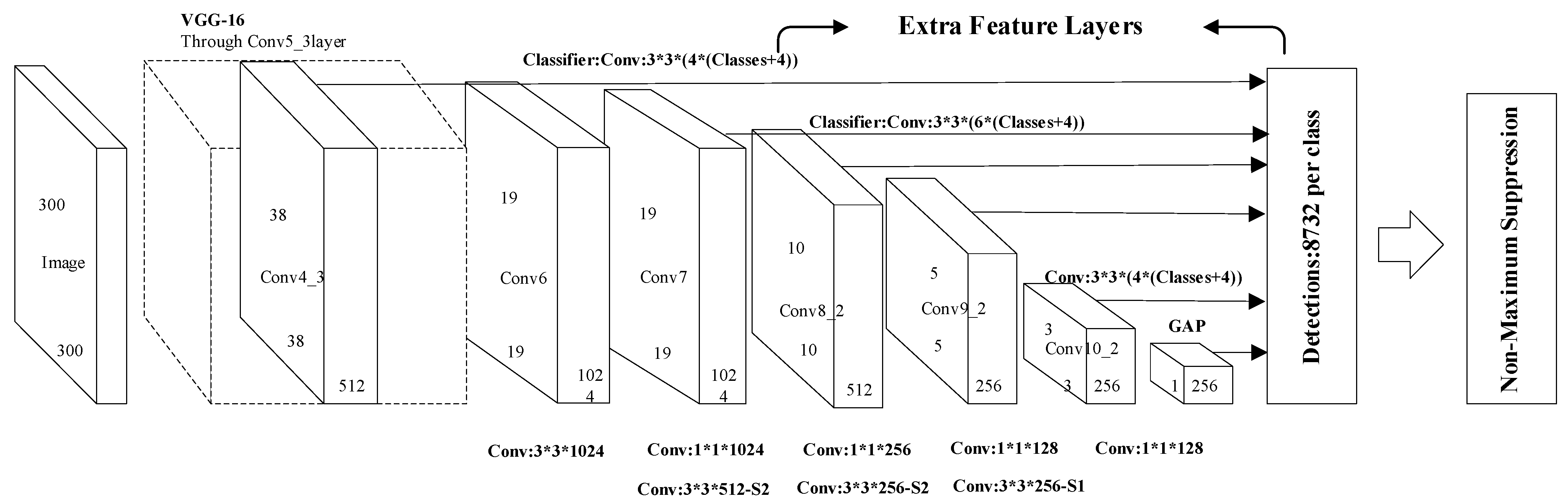
First, the basic structure of the remote sensing image target recognition network under low resolution is introduced. The basic structure of the remote sensing target recognition network used in this subject is shown in Figure 1. The basic network structure of the VGG16 is continued on the network backbone structure. The first five layers still use the five convolutional layers of the VGG16 network, discarding the fully connected layers of the sixth and seventh layers of the VGG16 network, while using the dilated convolution [38] method to construct two new convolution floors.
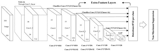
Figure 1.
Basic structure of low-resolution remote sensing image recognition network.
The conventional pooling layer in a deep neural network causes a decrease in resolution while increasing the receptive field, and the decrease in resolution causes a loss of some feature information. The advantage of this dilated convolution is to avoid the decrease in resolution caused by pooling [38]. The comparison between dilated convolution and ordinary convolution is shown in Figure 2. It can be seen from Figure 2 that under the same calculation parameters, a larger receptive field can be obtained by using dilated convolution instead of ordinary convolution.
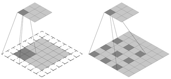
Figure 2.
Comparison of ordinary convolution (left) and dilated convolution (right).
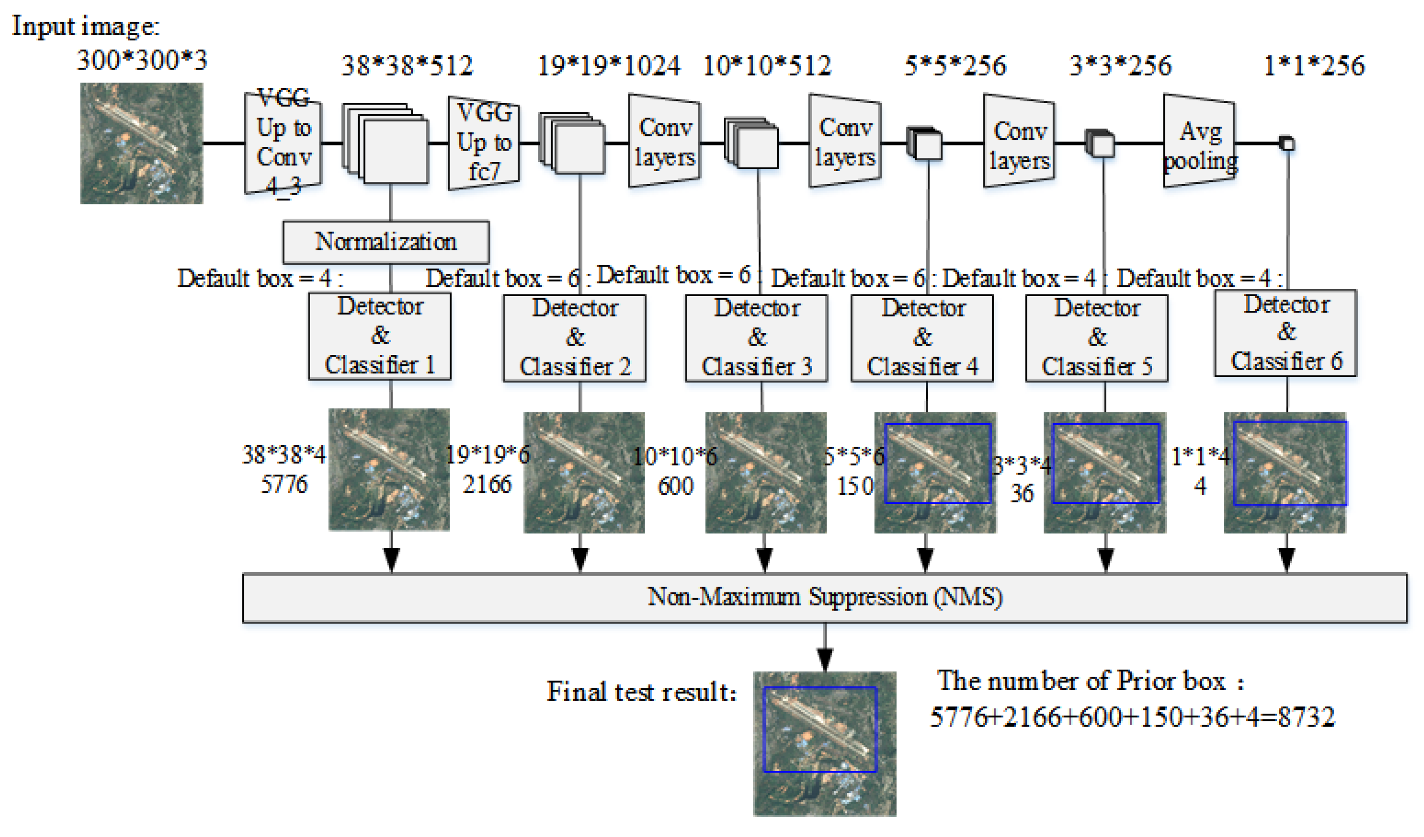
After the newly added sixth and seventh convolutional layers, three more convolutional layers (conv8, conv9, and conv10) are added, and a layer is added to the network at the end to convert the output feature map of the previous layer into a one-dimensional vector. For the remote sensing targets studied in this subject, there is a large intra-class gap for the same type of target, and there is still a problem of scale gap for the same type of target. Therefore, multi-scale recognition is particularly important. Considering the scale change of the target object, the network outputs feature maps of different scales at different layers and send them to the detector to predict the degree of confidence and position coordinate offset of each category. As shown in Figure 3, the front-most feature map is output after the Conv4_3 layer. The feature maps of the first few layers in the network describe the shallower features in the input image, and their receptive fields are relatively small. In contrast, the deeper feature maps are responsible for describing the more advanced composite features. Their lower-level feature maps of receptive fields are larger, and also have stronger advanced semantic information. At the end of the network, in order to avoid the result that the same target is detected by the multilayer feature detector at the same time, a non-maximum suppression process is added, as shown in Figure 3. From this, the final test result is obtained. The network backbone structure does not use a fully connected layer. On one hand, the output of each layer can only feel the characteristics of the area near the target, not the global information. On the other hand, it also reduces the number of computing parameters in the network.
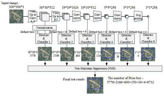
Figure 3.
Multi-scale detection in the network.
Step (2) Candidate box generation in the network
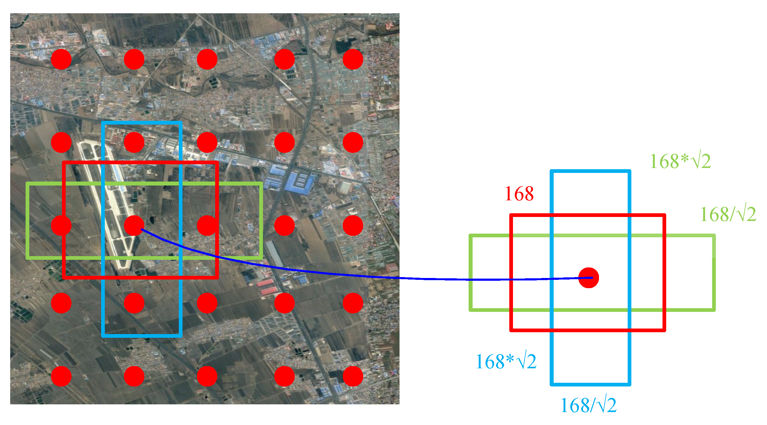
The network adopts an idea similar to Anchor in Faster R-CNN [33] to generate candidate regions, which is called the priority box here. For the aforementioned networks and for the six sets of feature maps generated by the Conv4_3, Conv7, Conv8_2, Conv9_2, Conv10_2, and global average pooling layers, the sizes are 38 × 38 × 512, 19 × 19 × 1024, 10 × 10× 512, 5 × 5 × 256, 3 × 3 × 256, and 1 × 1 × 256. For feature maps of different scale output by different layers, different aspect ratio candidate regions of the target object can be simulated by using different aspect ratios in each feature map. Figure 4 shows the process of generating priority boxes during airport image training in the network. Specific to the generation of each priority box, take the feature map of different scales. Taking Conv9_2 as an example, the size of the generated feature map is 5 × 5 × 256. Set its default box parameter to 6 in the network, that is, to generate 6 priority boxes with different aspect ratios around the same point around each anchor point. Then for the feature map of this layer, a total of 150 candidate priority boxes of 5 × 5 × 6 can be obtained for the prediction of category confidence and 4 position coordinate scores. In this network, for the output feature maps of each layer, the network generates 8732 priority boxes for prediction. In the process of network training, the prediction of an input image is equivalent to the prediction of classification and position regression of the 8732 sub-images of the input image at different scales.
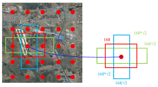
Figure 4.
Generation of candidate frames in the network.
In the process of generating boxes with different aspect ratios, two parameters of scale and ratio are used to control the generated boxes of different sizes. The scale parameter varies with the number of layers.
During network prediction, the scale value of the lowest-level feature map is set to 0.2, that is, Smin = 0.2, and the scale value of the highest-level feature map is set to Smax = 0.95. The ratio value interval is set to , and this parameter is used to control the aspect ratio of the candidate box around the anchor point. Use scale and ratio to calculate the size of the priority box in each layer feature map. Let the width of each priority box be and the height be . Then, the width and height of each priority box can be calculated by:
where Sk is a parameter of each layer, and its calculation formula is shown in:
For a ratio of 1, that is, an aspect ratio of 1, two candidate boxes with an aspect ratio of 1 are generated around each anchor point, and use extra to generate a box with an aspect ratio of 1. In this way, for each anchor point, you can get 6 different boxes.
Step (3) Network loss function design
The network in this topic belongs to a supervised learning network. For supervised learning, the target position and target category in the manually labeled labels are very important. In training, it is important to correlate artificially labeled target position category information with the boxes generated prior by the network. The first is about the definition of positive and negative samples. The concept of IoU is introduced here. For the target recognition task in this topic, as shown in Figure 5, the red dashed line on the left is the priority box generated during training, and the solid green line box is the target position manually labeled, where is the overlapping area of the two boxes and is the total area covered by the two boxes. Then, defining IoU is described as follows:
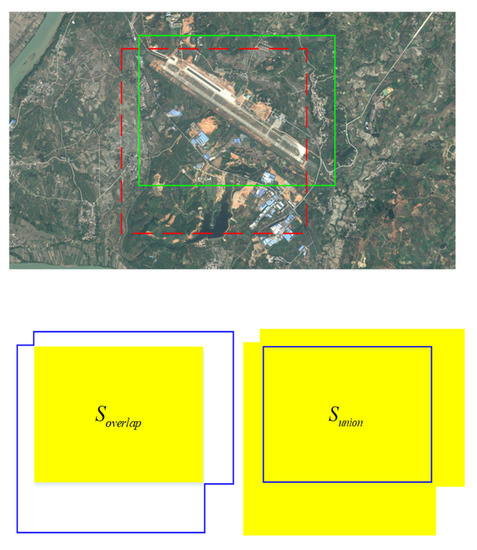
Figure 5.
IOU schematic.
During the training process, for several priority boxes generated by the network, if there are artificially labeled targets near the priority boxes, that is, ground truth, and the IOU of the box and ground truth is greater than 50%, the box is regarded as a positive sample; otherwise, it is considered a negative sample. Each box will have a certain positive and negative value. With this strategy, each ground truth corresponds to multiple positive samples, which also alleviates the problem of imbalance of positive and negative samples caused by too many negative samples during training.
During training, because there are two training purposes (category confidence and score prediction of four position parameters), the corresponding objective function is also divided into two parts. The objective function refers to the idea of multiBox loss function [39] and calculates the classification confidence of the category to which the target belongs and the regression accuracy of the target location. For the classification task for each box, the confidence calculation in the network is calculated using a softmax-type cross-entropy loss function. The specific calculation formulas are shown as:
The position loss regression function uses the calculation method of smooth L1-loss, and its loss function is shown as:
The total loss function in the network is the weighted sum of the above two loss functions as shown as:
where N is the number of positive samples.
Step (4) Network training strategy
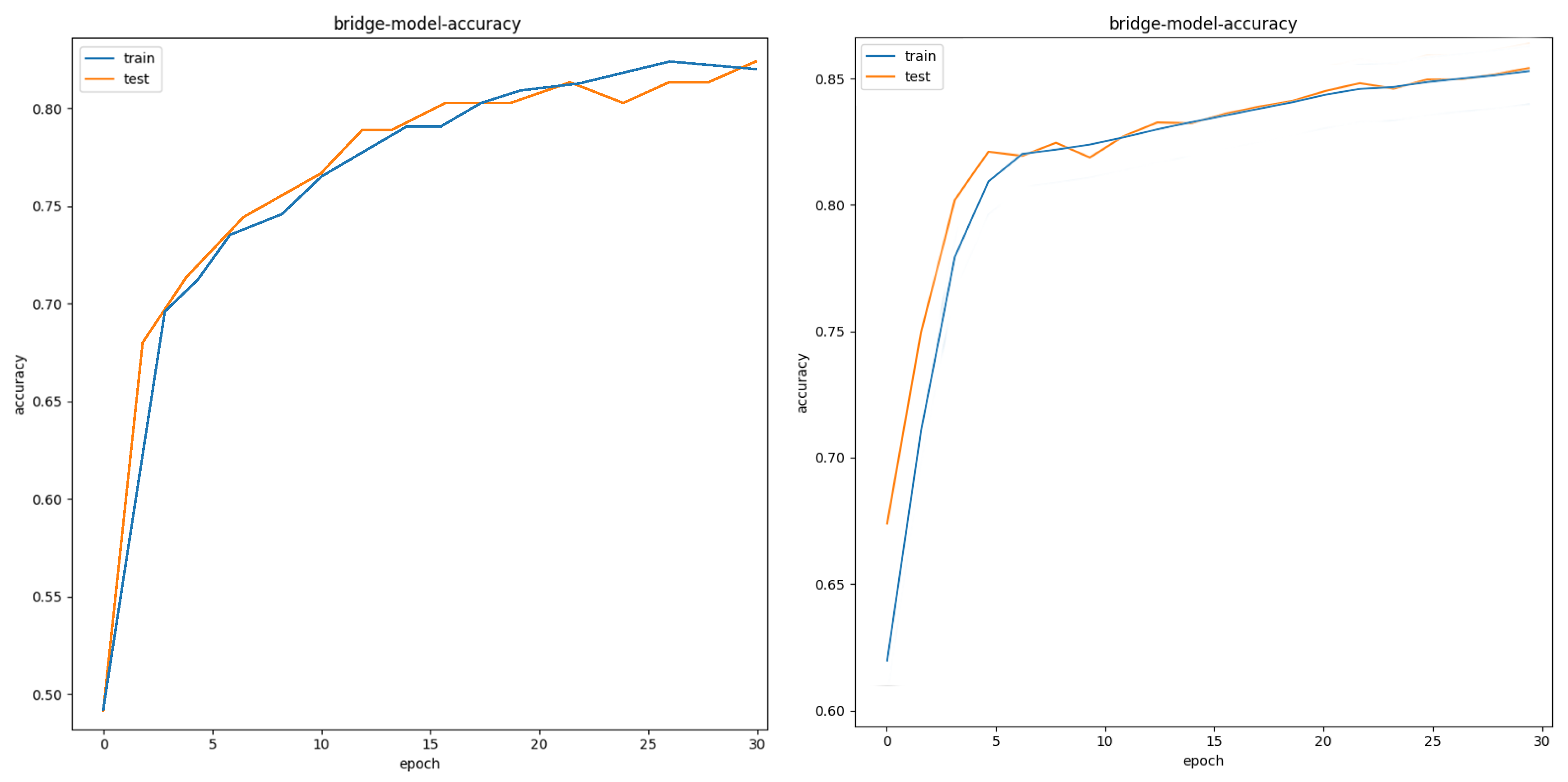
In response to the problem of insufficient data sets during the training process, this topic expands the following data sets, so that the number of labeled data was doubled, the expanded data set was trained, and the other training parameters were the same as the environment. In the case of the target dataset, after multiple experiments on the target data set, the data expansion improves the accuracy of target recognition by an average of 3 to 5 percentage points. Take airport training as an example: as shown in Figure 6, the left is the test accuracy before expansion, and the right is the recognition accuracy after data expansion.
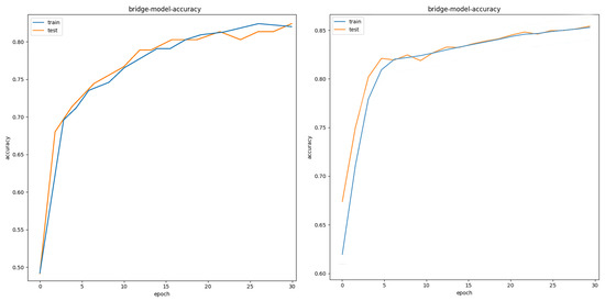
Figure 6.
Accuracy before and after data set expansion.
In the training process, because the priority boxes around each anchor point are mostly negative samples, if the original positive and negative samples are directly trained, the proportion of positive and negative samples is extremely imbalanced, and too many negative samples will affect the accuracy of training network to a certain extent. Therefore, the Hard Example Mining method is used in the training process to balance the positive and negative samples to a certain extent. The priority boxes with an IOU greater than 50% are regarded as positive samples, and during the training process, the Loss values of the class loss functions of all boxes will be sorted for each type of target, and the one with the largest Loss value will be selected. Some samples are used as negative samples, and the ratio of positive and negative samples is finally controlled to 1:3.
In the initialization stage of training, for the convolutional layers other than the newly added VGG16 convolutional layer, the initialization process of the weight in the convolution kernel is performed using the Xavier initialization [40] method. During the training process, Adam (Adaptive Moment Estimation) [41] was selected as the optimization method instead of the commonly used stochastic gradient optimization (SGD) to optimize the model to accelerate the speed of model convergence. The Adam optimization algorithm is a weight update method based on a dynamic learning rate. It adaptively selects a suitable learning rate for different parameter states during training, making the learning convergence process more stable and faster. Among them, the initial learning rate, impulse, weight attenuation, and other parameter values are slightly different according to different data sets in practice.
In addition, in order to improve the training results of the algorithm, this topic introduces transfer learning to improve the training recognition rate. Although the data set has been greatly expanded, the amount of data is still insufficient for deep recognition networks. For low-level feature extraction networks, the introduction of transfer learning can greatly improve the training results. Transfer learning focuses on training problems when there is insufficient data. The goal of transfer learning is to use the weight equivalents learned from a task to accelerate the learning and convergence process of a new task. With the help of transfer learning technology, a large number of existing data sets (such as the Pascal VOC data set) are directly used for pre-training, and then the parameters are loaded directly from the existing model during the training process. In the subject low-resolution remote sensing image target recognition algorithm, when a new target recognition training task is introduced, the existing model can be directly loaded to start training, thereby speeding up the convergence speed and improving the correct recognition rate to a certain extent. This method can also achieve the purpose of incremental learning of existing models required by technical indicators.
During the test process, since more than 8000 candidate regions were obtained to frame the same target for different priority boxes at different scales. For each output target area, non-maximum suppression is used to merge the target bounding boxes, sort by score, select the box with the highest score, and then calculate the other target boxes in the surrounding area and the highest score of IOU. Delete all boxes larger than a certain threshold, and then continue the previous process for all unbound bounding boxes until the final target box is obtained.
2.2. Proposed Parallel Computation Framework
The overall architecture of the UAV target detection system for ground stations in this paper is shown in Figure 7. The system can be divided into three parts: data transmission to the ground station, deep learning local target detection, and global target stable display.
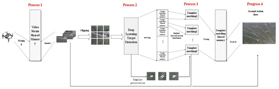
Figure 7.
Overall system flow.
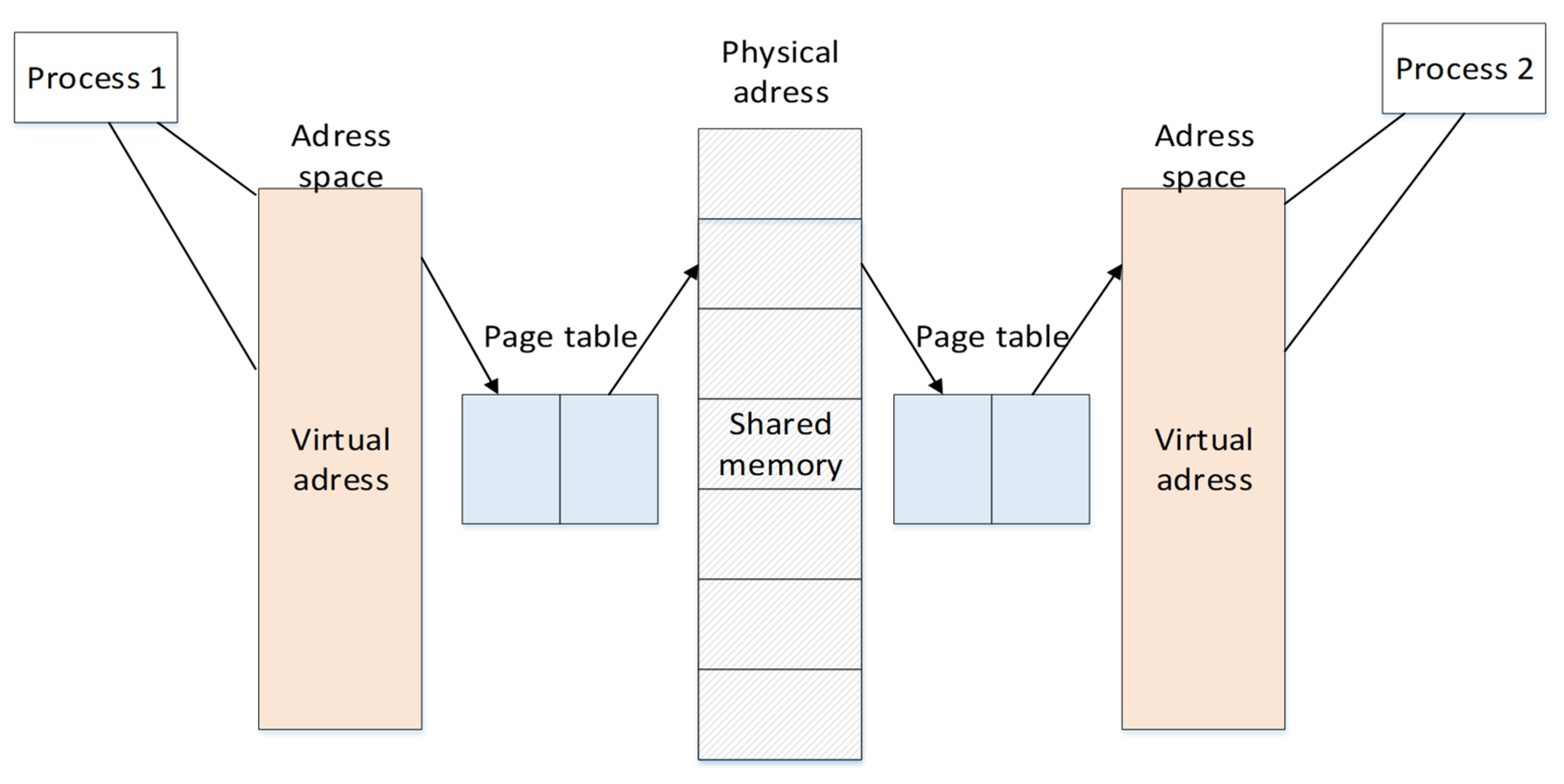
The three parts of the system operate independently but the information is related to each other, that is, the entire system is composed of four processes. Considering the overall real-time requirements of the system, the processes communicate with each other using shared memory. There are usually four ways of inter-process communication: pipes, semaphores, message queues, and shared memory. Shared memory is designed to solve the operational efficiency problem of inter-process communication, and is the fastest inter-process communication method. The basic communication principle is shown in Figure 8.
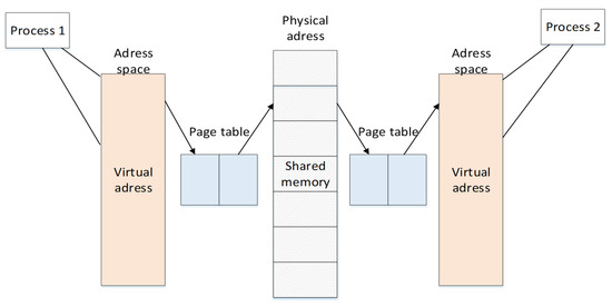
Figure 8.
Basic communication process of shared memory.
One of the methods used to realize the rapid transmission and sharing of data, images, and other information between two independent processes is to use the same physical address to store information, and each process accesses this address to obtain information of the other process. The process and the physical address of the shared memory connect their own virtual address space and actual physical space through a page table. As the data is directly stored in the memory, the frequency of multiple data replication for ordinary data transmission is reduced, thereby speeding up the transmission speed, and the time it takes to store information is almost negligible. Considering the requirements of this system, the writing and reading of information should be sequential, and only one process can access shared memory at a time between processes. Therefore, a mutex variable lock mechanism is added to achieve mutual access between processes.
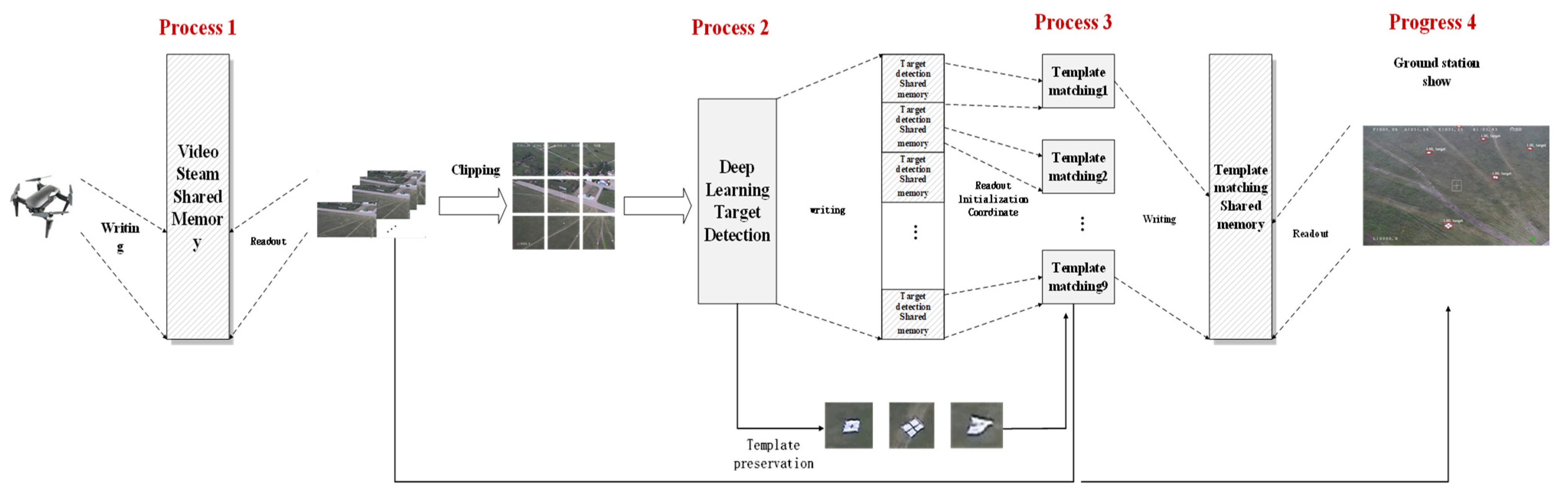
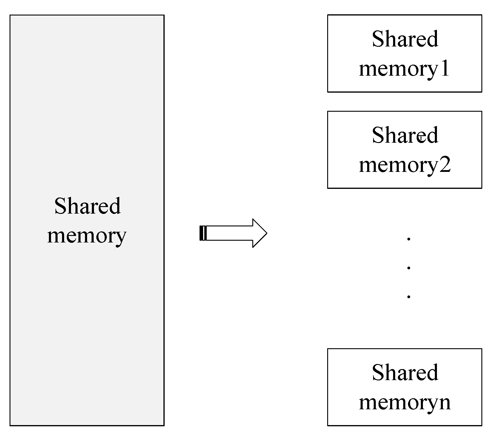
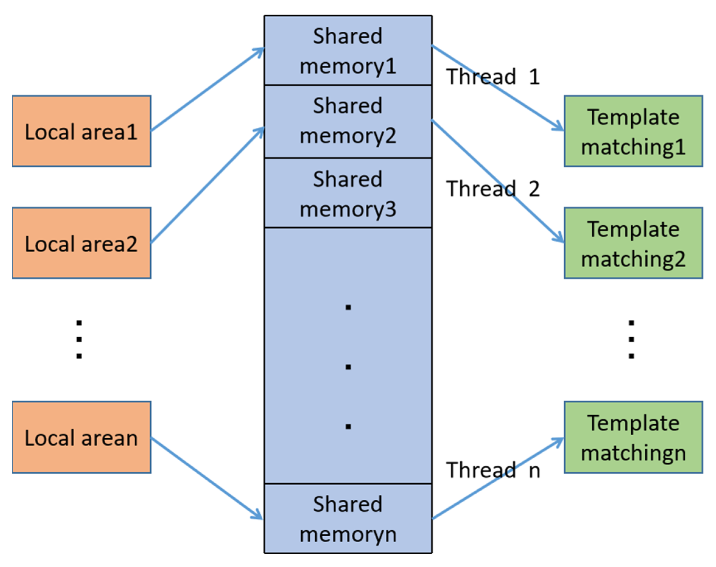
A total of four shared memory methods were used for information transfer between the four processes in this paper. First, the video data collected by the drone is shared with the ground station in real-time using a memory space used to store the original video stream data. Second, the initial position information and target slice information of the original video after deep learning local detection are stored in the second shared memory, which is different from the first shared memory, a shared memory for storing local target information divided according to the image. The number of local areas is decomposed into corresponding multiple sub-shared memory areas, as shown in Figure 9. Then, considering the stability and long-term nature of the detection results, the information of each child shared memory is used for subsequent further supplementation, screening, and fusion. After the final processing, it is stored in the last complete shared memory area, which is used to display the global target detection results.
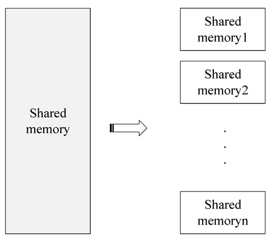
Figure 9.
Specific form of shared memory.
Through the design of the above framework, the entire process from data acquisition and target detection processing to stable and real-time display of the final detection result is realized. A complete system that can be applied to the target detection of actual UAV ground stations is set up.
The time complexity determines the training/prediction time of the model. If the complexity is too high, it will lead to a lot of time for model training and prediction, which can not quickly verify the idea and improve the model, nor can it achieve rapid prediction. The time complexity of this paper is defined as:
The spatial complexity determines the number of parameters of the model. Due to the limitation of the dimension curse, the more parameters of the model, the greater the amount of data required to train the model. In contrast, the data set in real life is usually not too large, which will make the model training easier to over fit. The spatial complexity of this paper is defined as:
3. Global and Local Joint Target Detection Method
3.1. Local Object Detection Method Based on Deep Learning
In view of the advantages of deep learning in the field of image processing and the development of current target detection directions, this paper uses deep learning algorithms for the preliminary processing of UAV image target detection.
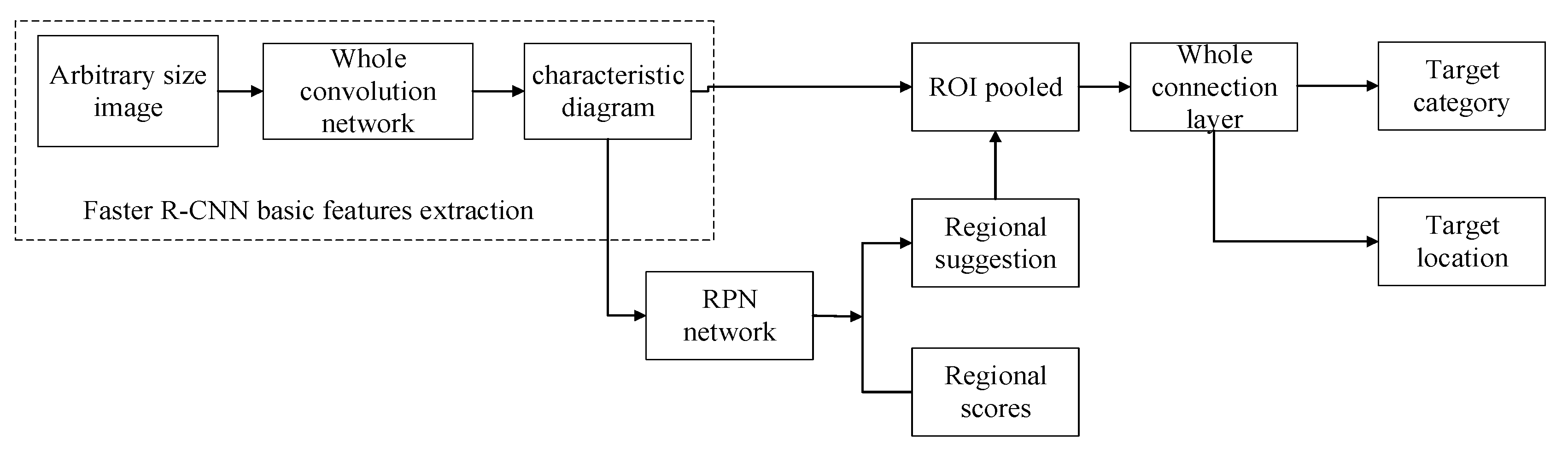
At this stage, there are mainly two types of deep learning networks used for object detection. One is a two-step target detection network R-CNN series that combines feature extraction and classification. At present, the Faster R-CNN network has the best effect of this type of network. The second is the single-step target detection SSD and YOLO [34] series using regression thinking. The Faster R-CNN network innovatively replaces the original brute force sliding window scanning methods such as selective search in the candidate area with the RPN network. The basic algorithm flow is shown in Figure 10.
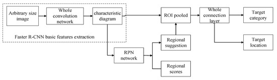
Figure 10.
Faster R-CNN algorithm flow.
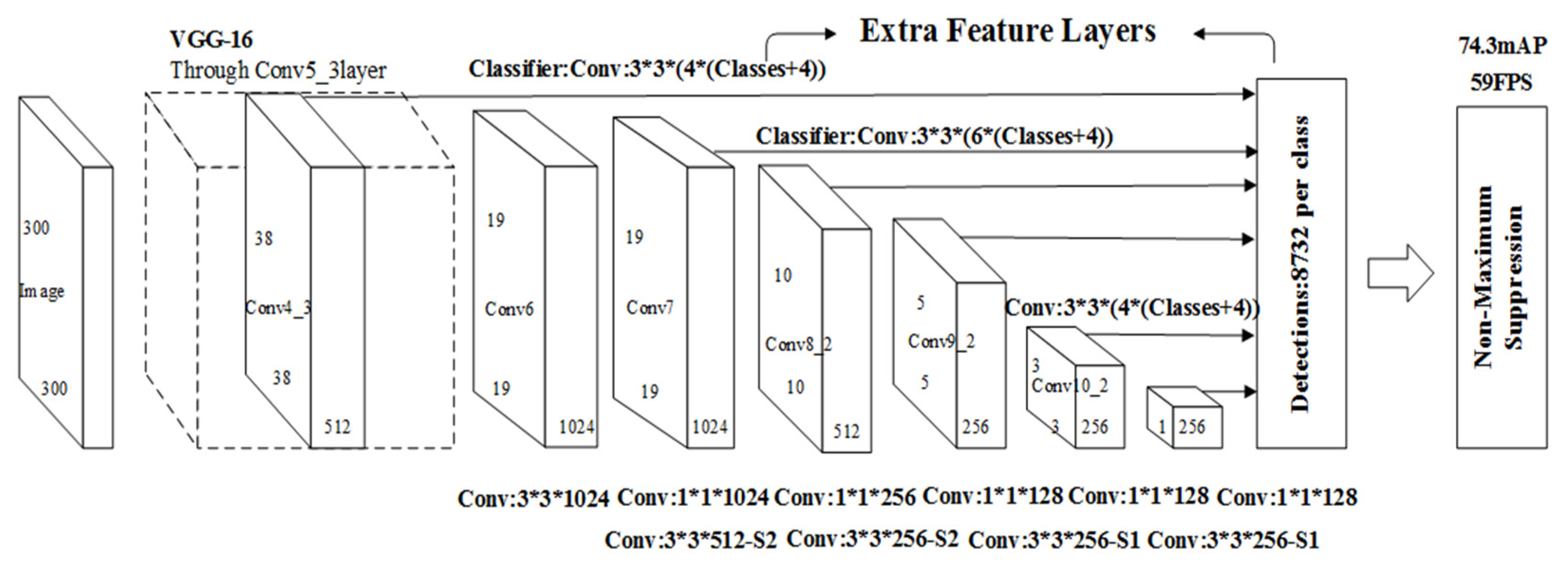
The basic features of the image are extracted using the full convolutional network. The RPN network constructed is then used to slide the window on the feature map for object front and back classification and frame position regression, and then further refined ROI pooling to obtain a more precise location of the frame. The Faster R-CNN network has a good accuracy rate, but because of the large number of candidate frames and other factors, the processing speed is very slow and cannot be applied to actual video-level processing. Figure 11 shows the basic network structure of SSD. The SSD network uses anchor points to output a series of discretized candidate frames. By combining feature maps at different levels, it ensures that the SSD network fully extracts the features of the target; taking different scales into consideration, and because the anchor points are designed with a variety of different aspect ratios, the SSD network can adapt to targets of multiple scales. This design of anchor points combined with feature pyramids improves the accuracy of the network in detecting different targets, and the idea of regression greatly improves the speed of network detection. It is a high-quality choice with a good compromise between detection accuracy and speed.

Figure 11.
SSD network structure.
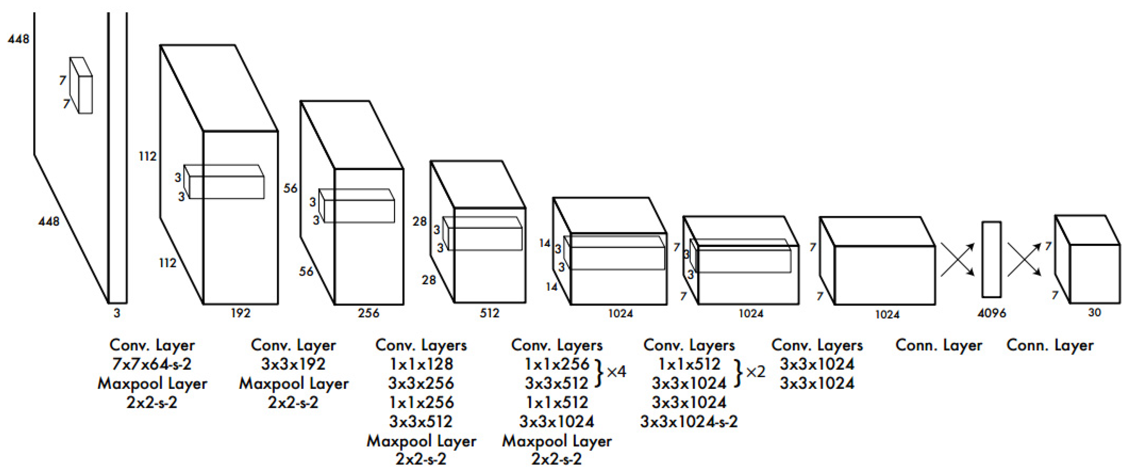
The YOLO network uses different ideas from the other two networks, and its algorithms are more direct and simpler [34]. The position of the candidate box and the corresponding category are directly returned in the output layer. The problem of target detection is thoroughly solved by regression. YOLO integrates target area prediction and target category prediction into a single neural network model to achieve fast target detection and recognition with high accuracy. The YOLO network architecture is shown in Figure 12. The YOLO network has a very high detection speed in object detection, but the detection accuracy rate is lower than other deep learning networks.
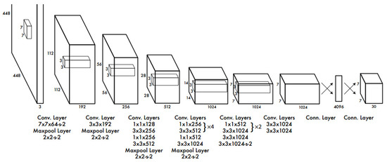
Figure 12.
YOLO network structure.
Table 1 lists the target detection results verified by the three networks on the PASCAL VOC dataset, mainly considering the average accuracy and speed.

Table 1.
Comparison of Deep Learning Object Detection Network Effects.
From Table 1, it can be seen that the recognition rate of Faster R-CNN is the best at present, followed by SSD, and the recognition rate of YOLO is lower; the recognition speed of YOLO is the fastest, in fact, and SSD and Faster R-CNN are the slowest. In order to verify the effect of the three networks in actual application scenarios, this paper uses self-built remote sensing image data to compare the three networks. The experimental platform is shown in Table 2.
Table 2.
Experimental platform.
The specific detection results of the six types of targets tested on the above platforms include ports, tanks, ships, aircraft, airports, and bridges, as shown in Table 3.
Table 3.
Verification of self-built dataset target detection network performance.
As shown in Table 4, the experimental results show that Faster R-CNN obtains the best recognition results. There are some misclassification cases, but the misclassification categories are generally evenly distributed in other categories, and there is no error in a particular category, indicating that the proposed feature is universal. However, its inference speed is significantly slower than the SSD network.
Table 4.
Confusion matrix-based Verification target detection network performance.
Comprehensive analysis shows that the SSD network has the best performance, which not only ensures the accuracy similar to Faster R-CNN but also achieves the same speed as the YOLO network. Therefore, this article chooses the SSD network as the detection network of the UAV ground station target detection system.
The target size of the aerial drone is less than 40 × 40 pixels at the minimum magnification. The SSD network has a limited effect on small target detection. The combination of the convolutional layer and the pooling layer in the feature extraction network design and downsampling the image multiple times will greatly reduce the image scale. The input size of a classic SSD network is 300 × 300, and the images collected by a drone usually have a higher resolution. The image size collected in this paper is 1920 × 1080 pixels, and the target only occupies a very small part of the image. When using an SSD network, the image must be scaled. The high-resolution image will lose a large amount of information after scaling and cause serious deformation of the target. Then it will be down-sampled multiple times by the network, resulting in loss of target features. Ultimately, there is very little target feature information for detection and recognition, which seriously affects the accuracy of detection. To this end, this article adopts the strategy of local detection of the image, first scaling the image to 900 × 900 pixels, and then dividing the image from top to bottom and left to right into nine subregions of 300 × 300. The SSD network processes only a sub-region of the current video frame image and completes the entire image detection after nine local processings. The specific process is shown in Figure 13.
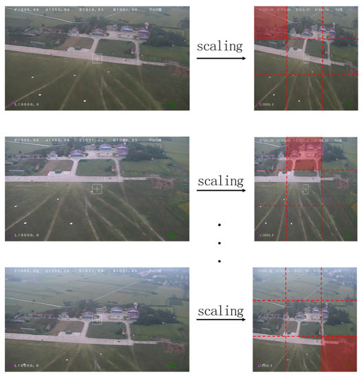
Figure 13.
Schematic diagram of local drone image detection process.
The SSD target detection network sequentially processes the local areas of each frame of the image. For example, the first frame of image processing detects the target of the first 300 × 300 area in the upper left corner, and the next frame sequentially processes the second upper left local areas of the second frame. The process is looped in turn until the local area detection of the ninth frame image is completed, and the next cycle is restarted. That is, a global detection is completed in nine frames.
By using the local loop detection method, the information loss of the original image is avoided from the input. This is especially of great significance for small target information retention. The target position information and slice information detected in each local area are stored in nine sub-shared memories corresponding to a shared memory, so as to facilitate further integration of the detection results in the future. This strategy can greatly improve the detection accuracy of local area targets, but it discards most of the global information. When the detection results are integrated and displayed at the end of each cycle, most target position and category information belong to historical frames. The drone is highly mobile, and the relative speed between the target and the drone is large due to its fast-moving speed, and the speed of the load acquisition image is higher than the speed of one cycle processing. This makes the displayed target position information lag behind the targets contained in the current frame image, and there is a large delay in visual observation. In view of the above problems, this paper proposes a global target detection information compensation strategy based on template matching.
3.2. Compensation of Global Target Detection Information Based on Template Matching
In order to meet the visual real-time requirements of drone video detection, a multithreading mechanism is added on the basis of the above research. At the same time, in order to facilitate the operator to perform subsequent advanced command operations based on the detection information, information such as the target position and category should be able to be displayed continuously and steadily. Therefore, further compensation detection processing is required for the areas not detected in each of the above frames. Considering the above two points, this paper combines the multi-threading mechanism and template matching detection algorithm to fine-tune and compensate for the target information detected by the SSD. The specific implementation process is shown in Figure 14.

Figure 14.
Compensation process for global target detection information.
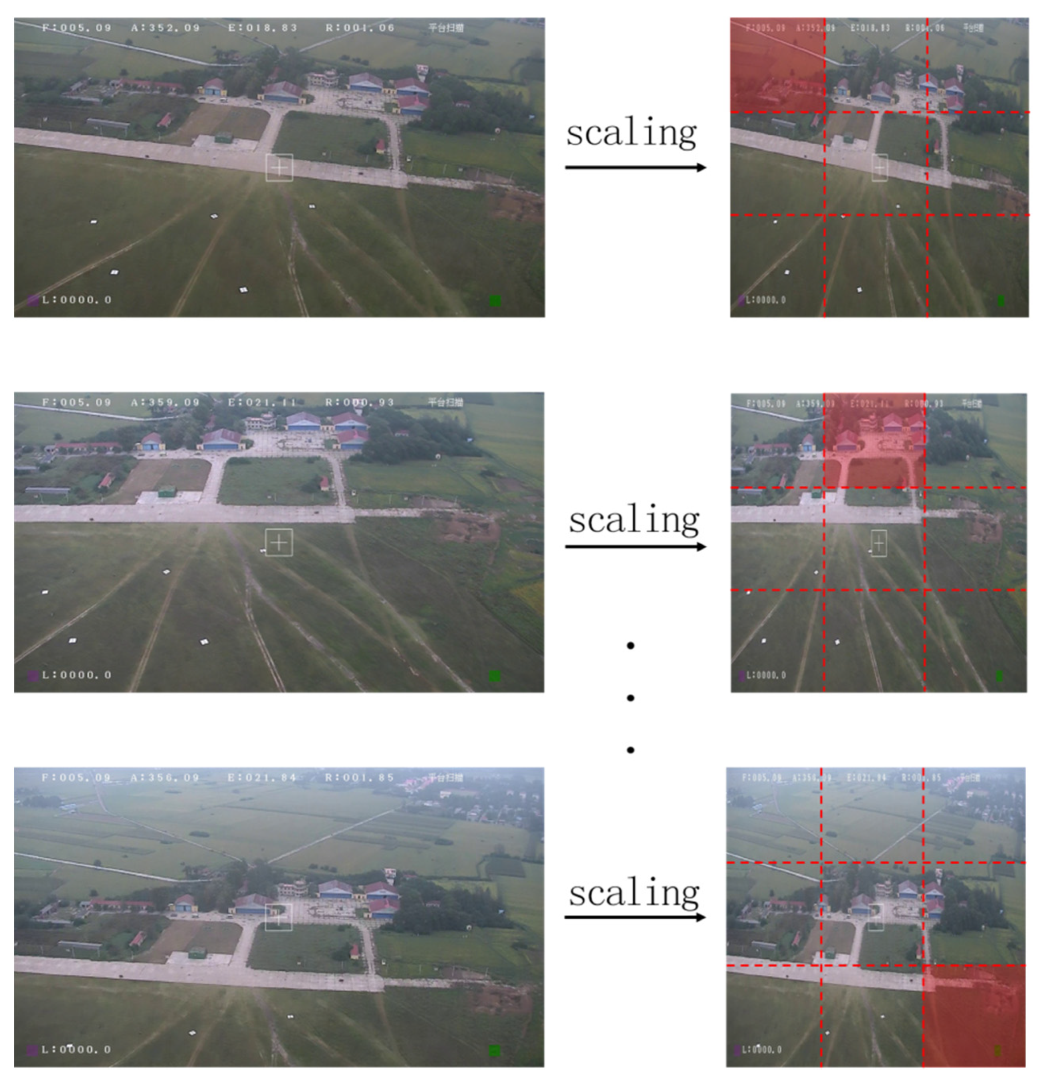
As shown in Figure 15, the main idea of template matching is with different scale-based image matching. A template matching algorithm is the easiest and fastest specific target matching technology in pattern recognition. Knowing the target matching template allows for search and match within the specified area to get the highest similar target position. The specific matching process is shown in Figure 15.

Figure 15.
Schematic diagram of template matching.
Start n multi-threads to monitor n shared memories. In this paper, the image is divided into nine local areas, so nine processes are started to manage shared memory. Each thread is responsible for the information compensation of a local area and uses nine template matchings to perform target detection on the local area. The multi-threaded template matching process and the SSD local area target detection process run independently. However, information is shared through shared memory, which mainly includes target location information, category information, target slices, etc.
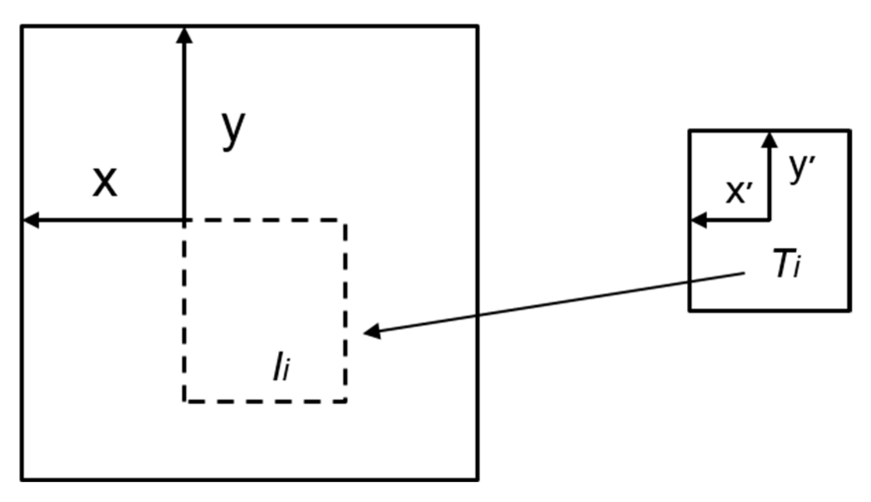
The template image is T, the original image is I, the most similar area to the template T is searched in the image I, and the final matched matrix is saved as R. The specific algorithm selected in this paper is the normalized correlation coefficient matching method. The image matrix obtained by matching at position (x, y) is :
Among them, the template image comes from two parts, one is the local area detection result of the SSD; the other is the last matching result. The coordinates of the target position detected in the local area are coordinates within the range of 300 × 300. In order to determine the template matching search position range, the local coordinates are mapped to the corresponding position of the original image of 1920 × 1080 pixels. The search area for template matching is determined to be centered on the target global coordinate center point position in the template, and the length and width are 5–8 times the range of the original template. If the search range is set too large, it will increase the matching time. The accumulation of time caused by multi-target matching will cause system delay; due to the relative movement between the drone load and the target, the search range is too small, and the target is not within the specified search range, the match will fail. The matching range of this paper is determined by many experiments, and the matching similarity threshold is set to 0.6.
Multi-process image templates are matched and synchronized without interference. When the SSD performs local target detection, nine processes monitor the corresponding changes in the corresponding nine shared memory sub-regions simultaneously. When the local detection of the SSD is completed, the corresponding shared memory information is updated to the newly detected target information, and the threads monitoring this shared memory area synchronize and update the template to continue matching. Otherwise, the template image and location information are unchanged, and template matching is performed continuously. Regardless of whether the subsequent detection successfully detects the target, once the first template matching starts, it will not end until the entire system detection ends. The SSD local detection is only responsible for updating the template for the corresponding thread template.
After this operation, the detection result of each frame of image includes the current local detection target of the SSD and other regional target matching results after template matching using the historical frame template. It makes full use of all the information of each frame image to make the detection result more fine and stable, and uses the multi-thread mechanism to improve the overall detection speed of the system, and achieves a balance between detection accuracy and speed.
3.3. Global Information Integration and Ground Station Display
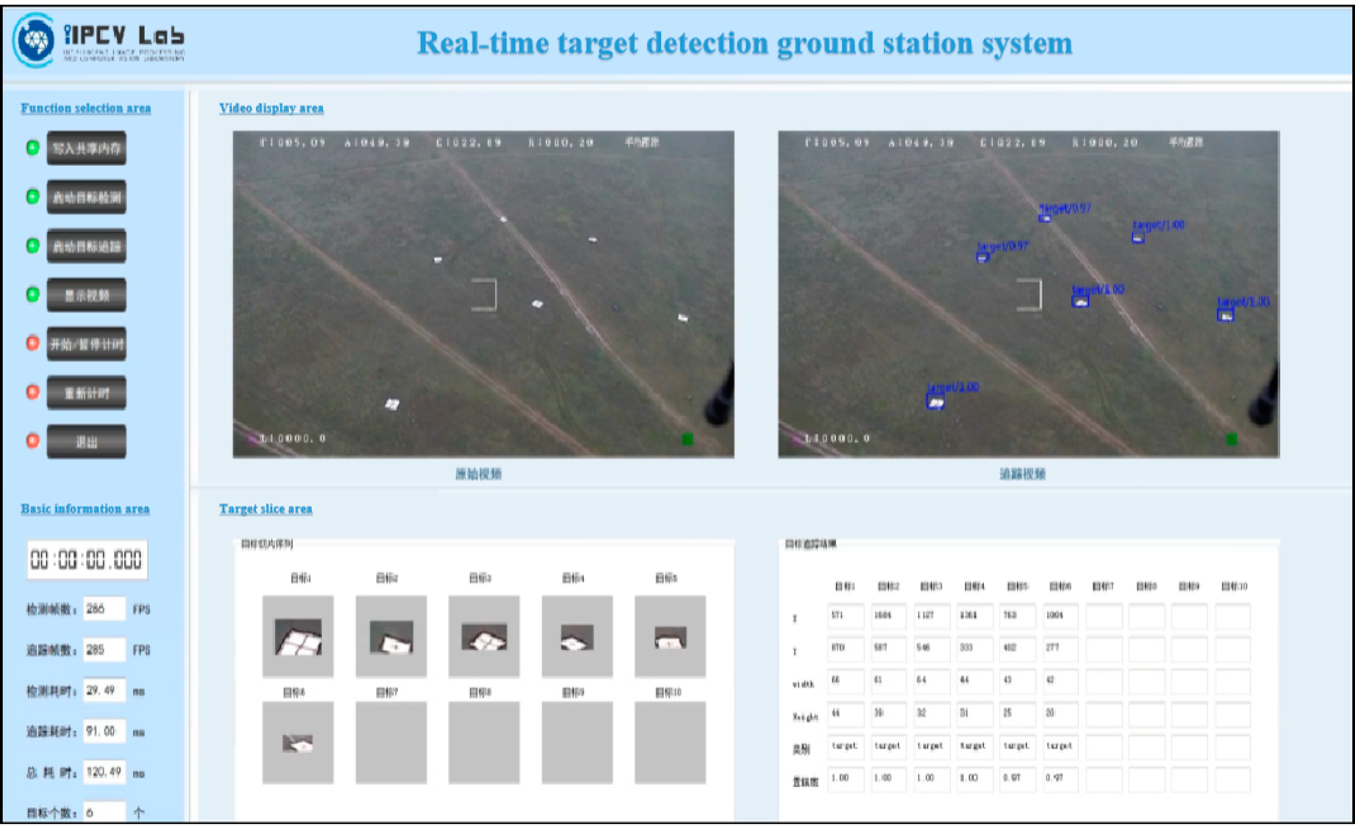
The detection and matching results between different local areas have a large number of duplicates. After integrating the results of the nine threads, Non-Maximum Suppression (NMS) processing is used to filter out multiple repeated boxes of the same target. This sorts multiple positioning boxes of the same target according to the category confidence and discards the positioning boxes whose IOU with the maximum confidence positioning box is greater than 0.7. Then, the remaining frame information after filtering the duplicate frames is sent to the shared memory. The ground station display system displays the target detection results of the input video in real-time by accessing the shared memory. The display interface design of this article is shown in Figure 16.
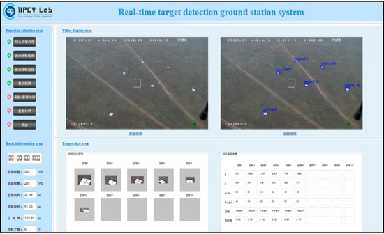
Figure 16.
Drone ground station display interface.
4. Experimental Verification of Algorithm Performance
4.1. Verification Conditions
(1) Data conditions
The data used in this article was obtained from an actual shooting at a test site in September 2018. Using a small rotary drone with a field of view angle of 20 degrees at a load field of view, a horizontal rotation speed of 5 degrees, and a vertical distance of 100 m from the ground to the target, a high-resolution image with a size of 1920 × 1080 pixels was obtained. The target to be tested in this paper is a cross-shaped target cloth with black or red lines on a white background. The actual size of the target cloth is 3 m × 3 m, which is uniformly identified as the target cloth. The relative motion between the target and the drone is generated by the drone flying at a constant speed. The target scale change is caused by the change in the distance of the drone load camera. This article contains the target cloth data when the camera focal length is changed from one to ten times. The specific target appearance is shown in Figure 17.
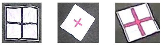
Figure 17.
Target appearance.
(2) Operation platform
In order to verify the effectiveness of the method, the software and hardware platforms used in this paper are: CPU: Intel(R) Core(TM) i7-6700 CPU @ 3.4 GHz; Memory: 16.0 GB; GPU: GeForce GTX 980; Display memory: 8.0 GB; System version: Windows 7 Professional. The deep learning framework is Caffe under Windows.
4.2. Experimental Process
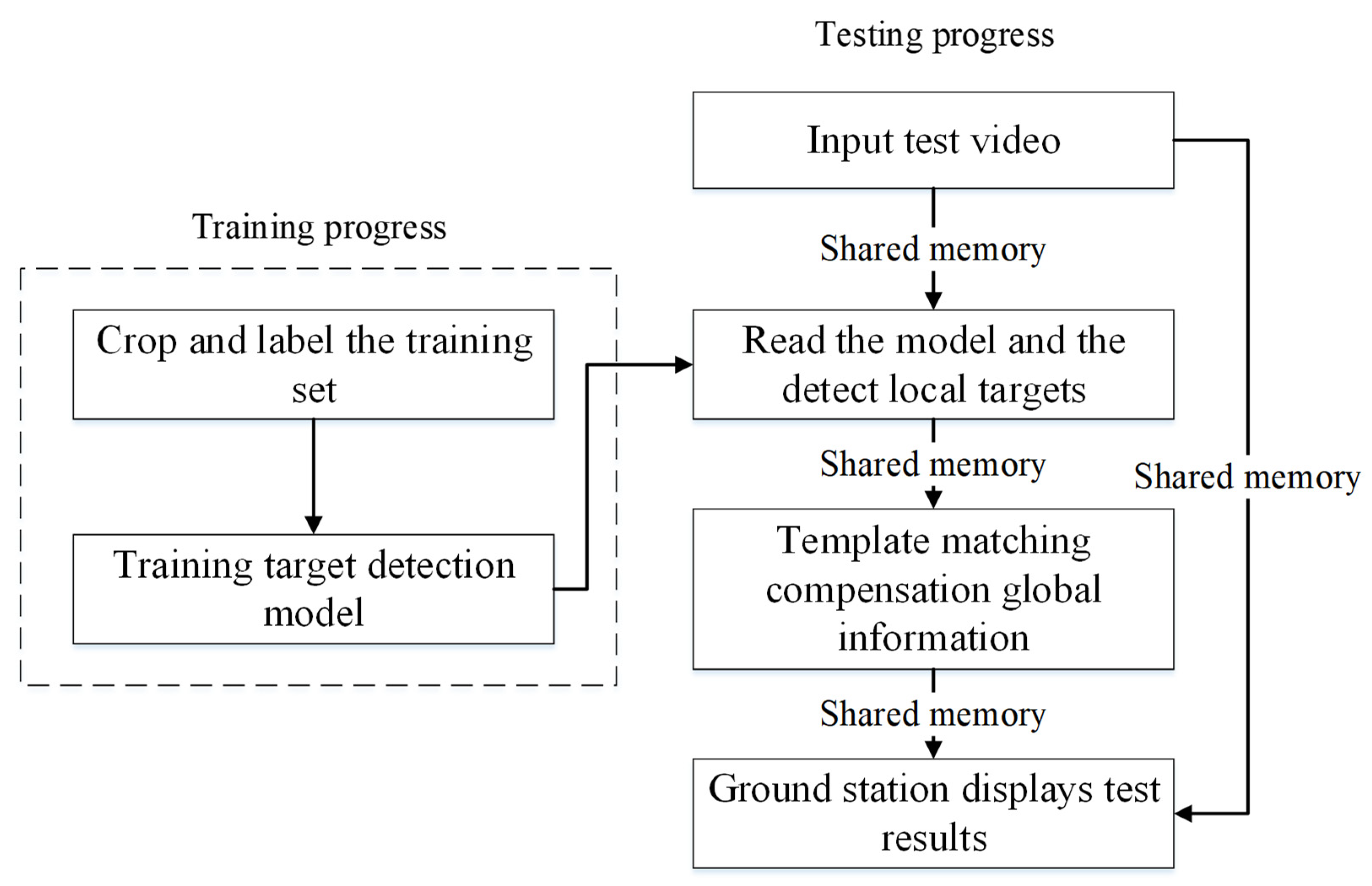
The specific verification process of this paper is shown in Figure 18.
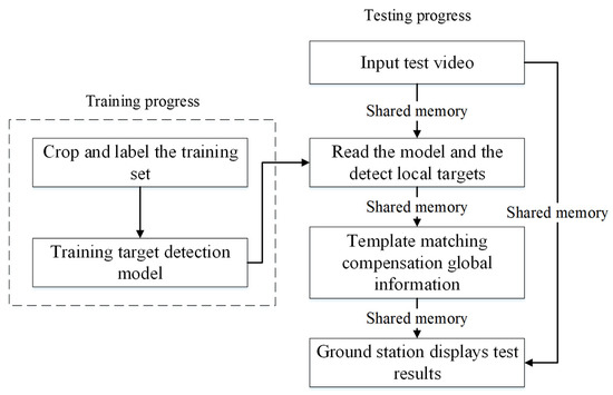
Figure 18.
Overall process of verification test for UAV ground station system.
The test is divided into two processes: SSD target detection network model training and testing the entire system using this model. Among them, before training the model, a training data set needs to be constructed. The training set samples are scaled to a size of 900 × 900 and then cropped into nine sub-region samples of 300 × 300 pixels arranged in a uniform order. The sub-sample target category and position information are labeled. The format of the labeled text is used by the standard Pascal VOC dataset (XML format). The target category is “target”.
The experimental dataset contains 14,817 samples, which are randomly divided into a training set and a validation set according to a ratio of 8:2. The number of training sets is 11,854, and the number of validation sets is 2963. The data covers images with the focal length of the camera ranging from one to ten times to adapt to target detection at multiple scales. The stochastic gradient descent (SGD) optimization method is used to solve the minimum loss function. The total number of training sessions is 80,000. Other training hyperparameter settings are shown in Table 5. Among them, the initial value of the learning rate is 0.001, and after 40,000 training sessions, the learning rate decays to 1/10 of the original.
Table 5.
Hyperparameter settings.
The test uses video captured by the drone as input. A piece of video containing 1 to 10 times a constant-speed video for 1 min and a total of 15,000 frames was selected. After starting four processes at the same time, the real-time video detection effect was observed and the detection result was saved locally for subsequent result analysis.
4.3. Experimental Results and Analysis
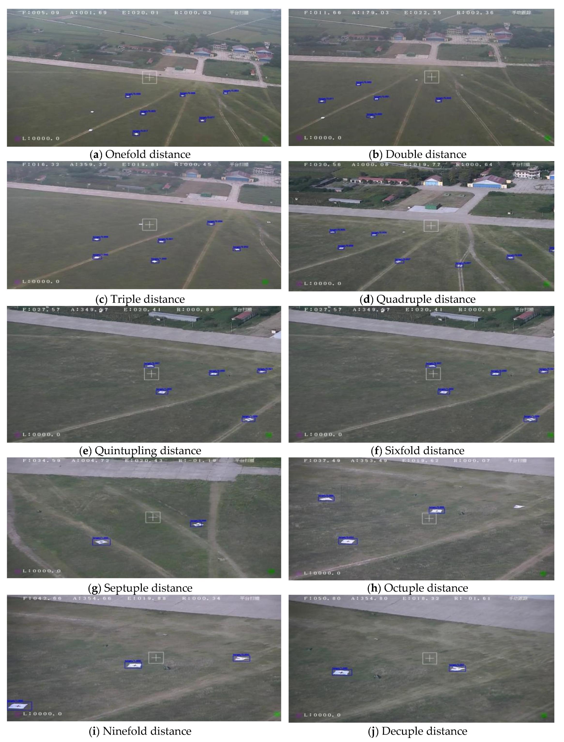
The detection results of continuous video targets using the UAV downward-looking ground station detection system designed in this paper are shown in Figure 19. Figures of detection results under one to ten times focal length changes are shown.
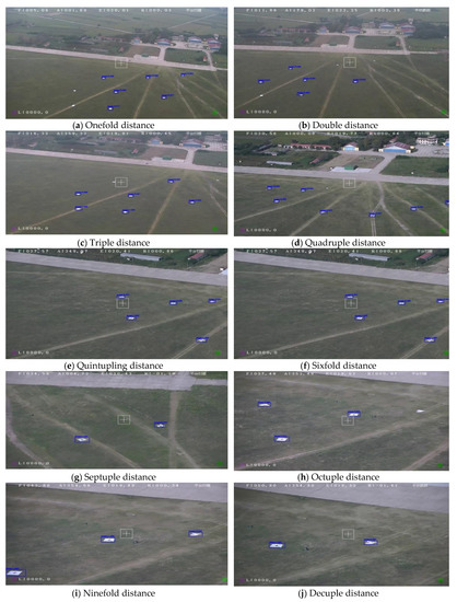
Figure 19.
Target detection results under change of focal length.
From the detection results shown in Figure 19, when the field of view is 20 degrees in non-vertical shooting, the shape of the target changes greatly. Before the focal length of the load camera is enlarged to five times, the target has missed detection, especially in the case of a large change in the appearance of the target, the missed detection is large. In addition, the smaller the focal length, the larger the number of targets in the field of view, and the more background interference objects, the greater the possibility of misdetection. After the focal length is increased to five times, the target’s appearance becomes clearer, the features become more prominent, the detection accuracy is relatively high, and the possibility of missed detection and false detection is also low. The test results for each multiple are shown in Table 6. Among them, the accuracy of target detection before five times the distance is less than 80%, and the frequency of false detection is higher; the accuracy of target detection after seven times the distance is higher than 95%, and the detection effect is better.
Table 6.
Statistics of test results at different magnifications.
The test time drawing of 3750 frames of images randomly selected is shown in Figure 20. The calculation shows that the average time for a test is 56.6 ms. When the system processing time fluctuates greatly, it is affected by multi-thread scheduling. The processing time of most images is below 75 ms, which can meet the real-time requirements of actual video detection.
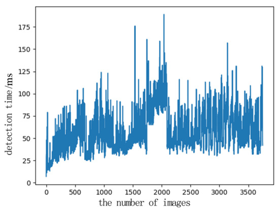
Figure 20.
Test time of the target detection system.
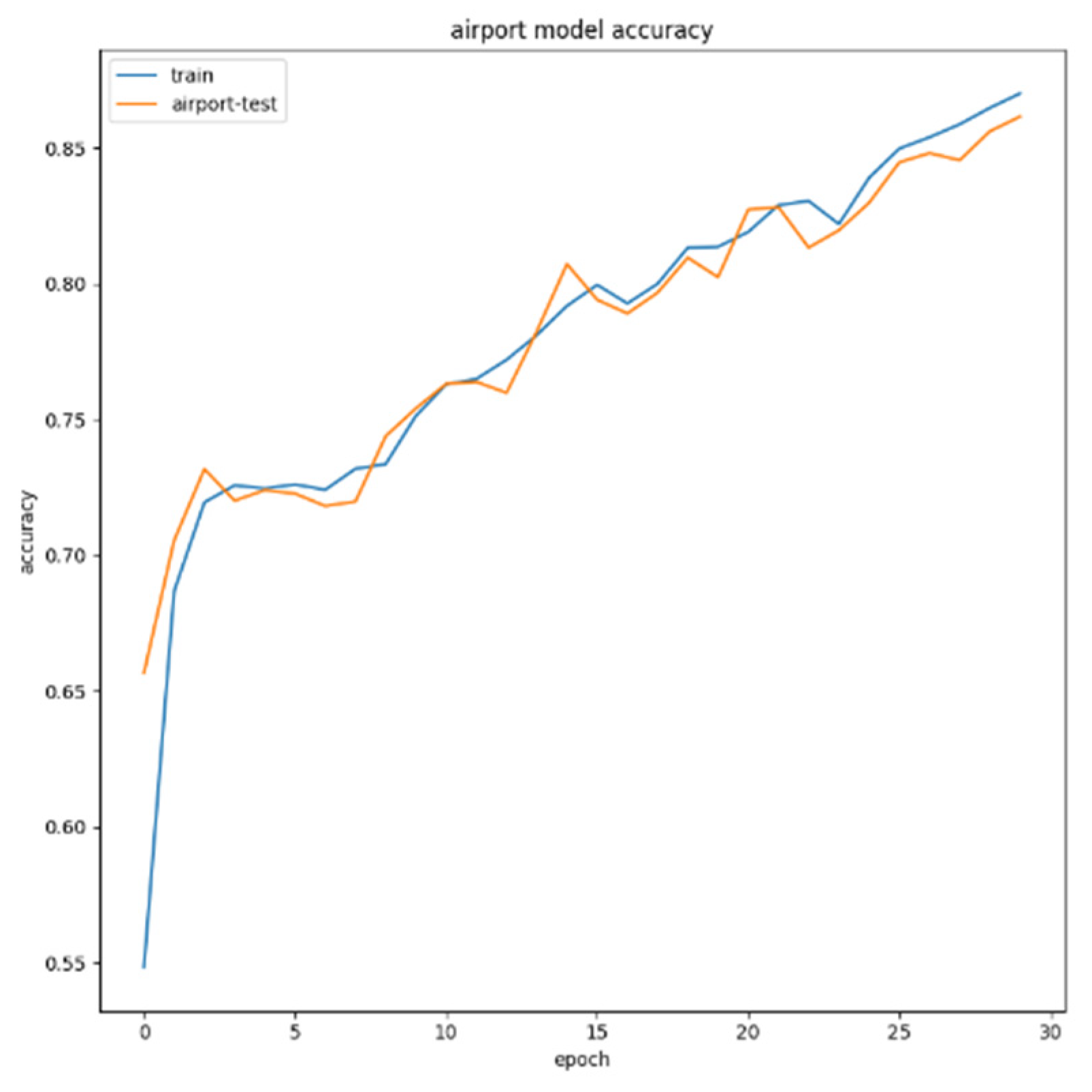
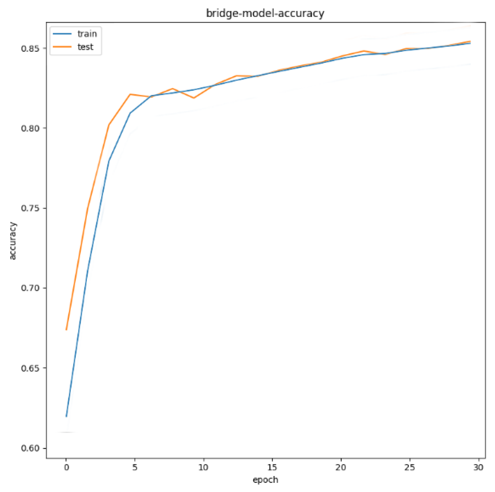
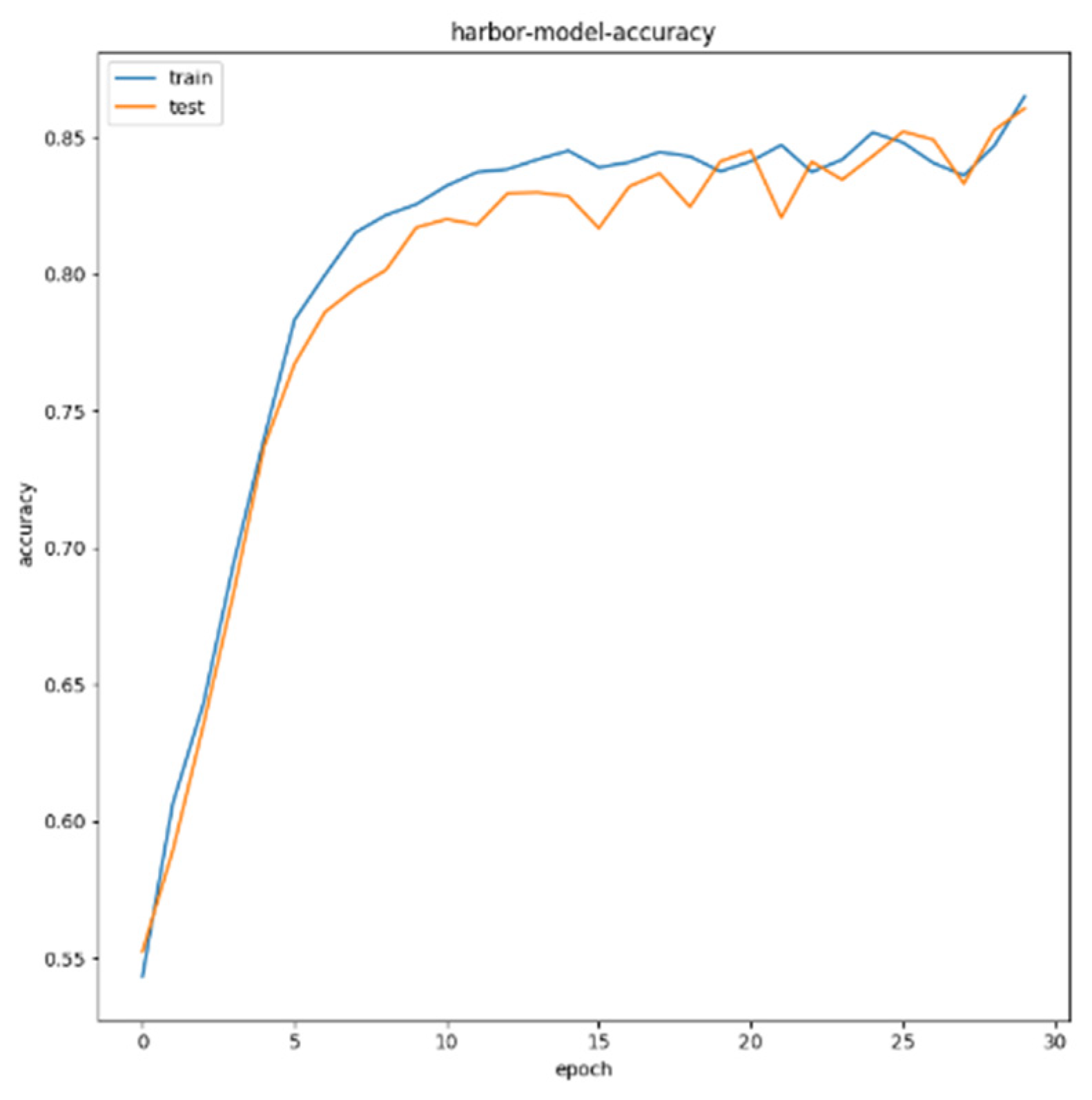
For airport targets, the test set is 100 test images containing airport targets. As can be seen from Figure 21, after 30 epochs, the recognition accuracy of the system for the airport in the test image reaches 86%; for bridge targets, the test set is 120 test images including airport targets. As can be seen from Figure 22, after 30 epochs, the bridge recognition accuracy reaches 86%; for bridge targets, the test set is 240 test images including airport targets. As can be seen from Figure 23, after 30 epochs, the port recognition accuracy reaches 87%.
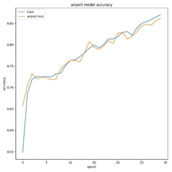
Figure 21.
Airport target recognition accuracy.
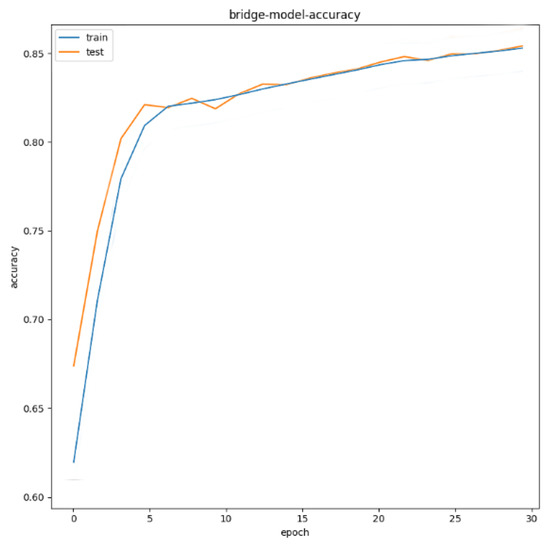
Figure 22.
Accuracy of bridge target recognition.

Figure 23.
Accuracy of port target recognition.
This section gives the comparison between the model designed in this paper and other popular target detection models and gives the acceleration effect of this model on the actual hardware platform after pruning and quantization. The floating point model in this paper is trained on the VOC dataset [37]; the number of training rounds was 80. Standard data enhancement methods were used, including random clipping, perspective transformation, and horizontal flipping. In addition, a mixup data enhancement method was used [42]. The Adam [41] optimization algorithm and cosine annealing learning rate strategy are adopted. The initial learning rate is 4 × 10⁻³ and the small batch size is 16. As shown in Table 7, the network at 512 × the input image size of 512, the VOC data set reaches 78.46% of the test set map. The model calculation amount is 4.24 G Macs and the model parameter amount is 6.775 M. See Table 7 for a comparison with other network models with regard to accuracy, calculation, and parameters. The proposed algorithm has high accuracy and low computation complexity.
Table 7.
Comparison of accuracy, calculation, and parameters between this model and other network models.
As shown in Table 8, it can be seen from the confusion matrix that the categories of the misclassified samples in the proposed algorithm are generally evenly distributed in other categories. The experimental results show that the proposed features are universal and do not specifically target the errors of a certain category.
Table 8.
Confusion matrix of the proposed target detection network performance.
All model data in Table 7 are in a 512 × 512 input image size, indicators on the VOC 2007 test set. Through comparison, the accuracy of the network model proposed in this paper is not much different from that of the YOLOv3 model, but the amount of calculation and parameters are greatly reduced. Compared with the YOLOv3 and YOLO Nano, the model in this paper still has great advantages in accuracy and calculation.
5. Conclusions
In this paper, aiming at the low accuracy of UAV video target detection and the inability to meet timelines, a complete UAV target detection system can be designed for ground stations. This system uses the combination of deep learning and traditional template matching to fully mine the local and global information of the image, and cleverly uses mechanisms such as multi-process and multi-thread to complete the rapid processing of information synchronization. The average detection rate is 86.1%, and the average detection time is 56.6 ms. Regardless of accuracy or processing speed, it can meet the actual application requirements.
Author Contributions
Conceptualization, J.C.; funding acquisition, J.C.; methodology, L.S.; project administration, J.C., D.F. and M.X.; validation, L.S.; writing—original draft, L.S.; writing—review and editing, J.C.; supervision, D.F. and M.X. All authors have read and agreed to the published version of the manuscript.
Funding
This research was supported in part by the Foundation for Innovative Research Groups of the National Natural Science Foundation of China under Grant 61621005, in part by the National Natural Science Foundation of China under Grant 62001003, in part by the Natural Science Foundation of Anhui Province under Grant 2008085QF284, and in part by the China Postdoctoral Science Foundation under Grant 2020M671851.
Institutional Review Board Statement
Not applicable.
Informed Consent Statement
Not applicable.
Data Availability Statement
Not applicable.
Acknowledgments
We would like to express our heartfelt thanks to anonymous reviewers and editors for their constructive comments on the paper.
Conflicts of Interest
The authors declare no conflict of interest.
References
- Liu, W.C.; Lu, C.H.; Huang, W.C. Large-Scale Particle Image Velocimetry to Measure Streamflow from Videos Recorded from Un-manned Aerial Vehicle and Fixed Imaging System. Remote. Sens. 2021, 13, 2661. [Google Scholar] [CrossRef]
- Zeng, Y.; Zhang, R.; Lim, T.J. Wireless communications with unmanned aerial vehicles: Opportunities and challenges. IEEE Commun. Mag. 2016, 54, 36–42. [Google Scholar] [CrossRef] [Green Version]
- Wang, Y.; Chen, M.; Yang, Z.; Luo, T.; Saad, W. Deep Learning for Optimal Deployment of UAVs With Visible Light Communications. IEEE Trans. Wirel. Commun. 2020, 19, 7049–7063. [Google Scholar] [CrossRef]
- Kim, D.; Lee, J.; Quek, T.Q.S. Multi-layer Unmanned Aerial Vehicle Networks: Modeling and Performance Analysis. IEEE Trans. Wirel. Commun. 2019, 19, 325–339. [Google Scholar] [CrossRef]
- Kratky, V.; Alcantara, A.; Capitan, J.; Stepan, P.; Saska, M.; Ollero, A. Autonomous Aerial Filming With Distributed Lighting by a Team of Unmanned Aerial Vehicles. IEEE Robot. Autom. Lett. 2021, 6, 7580–7587. [Google Scholar] [CrossRef]
- Wu, Z.; Suresh, K.; Narayanan, P.; Xu, H.; Kwon, H.; Wang, Z. Delving Into Robust Object Detection From Unmanned Aerial Vehicles: A Deep Nuisance Disentangle-ment Approach. In Proceedings of the 2019 IEEE/CVF International Conference on Computer Vision (ICCV), Seoul, Korea, 27–28 October 2019; pp. 1201–1210. [Google Scholar]
- Zhang, P.; Zhong, Y.; Li, X. SlimYOLOv3: Narrower, Faster and Better for Real-Time UAV Applications. In Proceedings of the 2019 IEEE/CVF Interna-tional Conference on Computer Vision Workshop (ICCVW), Seoul, Korea, 27–28 October 2019; pp. 1–9. [Google Scholar]
- He, Y.; Fu, C.; Lin, F.; Li, Y.; Lu, P. Towards Robust Visual Tracking for Unmanned Aerial Vehicle with Tri-Attentional Correlation Filters. In Proceedings of the 2020 IEEE/RSJ International Conference on Intelligent Robots and Systems (IROS), Las Vegas, NV, USA, 25–29 October 2020; pp. 1575–1582. [Google Scholar] [CrossRef]
- Chen, Z.; Liu, Y.; Zhai, S.; Li, X. Performance Evaluation of Visual Object Detection for Moving Vehicle. In Proceedings of the International CCF Conference on Artificial Intelligence, Xuzhou, China, 22–23 August 2019; pp. 131–144. [Google Scholar] [CrossRef]
- Cao, W.; Yuan, J.; He, Z.; Zhang, Z.; He, Z. Fast Deep Neural Networks With Knowledge Guided Training and Predicted Regions of Interests for Real-Time Video Object Detection. IEEE Access 2018, 6, 8990–8999. [Google Scholar] [CrossRef]
- Ramli MF, B.; Legowo, A.; Shamsudin, S.S. Object Detection Technique for Small Unmanned Aerial Vehicle. Mater. Sci. Eng. 2017, 260, 012040. [Google Scholar]
- Qin, R. An Object-Based Hierarchical Method for Change Detection Using Unmanned Aerial Vehicle Images. Remote. Sens. 2014, 6, 7911–7932. [Google Scholar] [CrossRef] [Green Version]
- Kamate, S.; Yilmazer, N. Application of Object Detection and Tracking Techniques for Unmanned Aerial Vehicles. Procedia Comput. Sci. 2015, 61, 436–441. [Google Scholar] [CrossRef] [Green Version]
- Jaiswal, D.; Kumar, P. Real-time implementation of moving object detection in UAV videos using GPUs. J. Real-Time Image Process. 2019, 17, 1301–1317. [Google Scholar] [CrossRef]
- Han, F.; Shan, Y.; Cekander, R.; Sawhney, H.S.; Kumar, R. A Two-Stage Approach to People and Vehicle Detection with HOG-Based SVM. Perform. Metr. Intell. Syst. 2006, 2006, 133–140. [Google Scholar]
- Choi, J.Y.; Sung, K.S.; Yang, Y.K. Multiple vehicles detection and tracking based on scale-invariant feature transform. In Proceedings of the 2007 IEEE Intelligent Transportation Systems Conference, Seattle, WA, USA, 30 September–3 October 2007; pp. 528–533. [Google Scholar]
- Viola, P.; Jones, M. Rapid Object Detection Using a Boosted Cascade of Simple Features. In Proceedings of the 2001 IEEE Computer Society Conference on Computer Vision and Pattern Recognition, CVPR 2001, Kauai, HI, USA, 8–14 December 2001; pp. 511–518. [Google Scholar]
- Sokalski, J.; Breckon, T.P.; Cowling, I. Automatic salient object detection in uav imagery. In Proceedings of the 25th International Unmanned Air Vehicle Systems, Bristol, UK, 12–14 April 2010; pp. 11.1–11.12. [Google Scholar]
- ElTantawy, A.; Shehata, M.S. Local null space pursuit for real-time moving object detection in aerial surveillance. Signal Image Video Process. 2019, 14, 87–95. [Google Scholar] [CrossRef]
- Konoplich, G.V.; Putin, E.O.; Filchenkov, A.A. Application of deep learning to the problem of vehicle detection in UAV images. In Proceedings of the 2016 XIX IEEE International Conference on Soft Computing and Measurements (SCM), St. Petersburg, Russia, 25–27 May 2016; pp. 4–6. [Google Scholar]
- Barrero, O.; Rojas, D.; Gonzalez, C.; Perdomo, S. Weed detection in rice fields using aerial images and neural networks. Images Artif. Vis. 2016, 15, 1–4. [Google Scholar] [CrossRef]
- Zhang, P.; Niu, X.; Dou, Y.; Xia, F. Airport Detection on Optical Satellite Images Using Deep Convolutional Neural Networks. IEEE Geosci. Remote. Sens. Lett. 2017, 14, 1183–1187. [Google Scholar] [CrossRef]
- Xiao, Z.; Gong, Y.; Long, Y.; Li, D.; Wang, X.; Liu, H. Airport Detection Based on a Multiscale Fusion Feature for Optical Remote Sensing Images. IEEE Geosci. Remote. Sens. Lett. 2017, 14, 1469–1473. [Google Scholar] [CrossRef]
- Li, T.; Zhang, J.; Zhang, Y.; Jiang, L.; Li, B.; Yan, D.; Ma, C. Fast and Accurate, Convolutional Neural Network Based Approach for Object Detection from UAV. In Proceedings of the IECON 2018–44th Annual Conference of the IEEE Industrial Electronics Society, Washington, DC, USA, 21–23 October 2018; pp. 3171–3175. [Google Scholar]
- Robicquet, A.; Sadeghian, A.; Alahi, A.; Savarese, S. Learning Social Etiquette: Human Trajectory Understanding. Crowded Scenes 2016, 9, 549–565. [Google Scholar] [CrossRef] [Green Version]
- Krizhevsky, A.; Sutskever, I.; Hinton, G.E. ImageNet classification with deep convolutional neural networks. In Proceedings of the Conference and Workshop on Neural Information Processing Systems (NIPS), Lake Tahoe, NV, USA, 3–6 December 2012; pp. 1097–1105. [Google Scholar]
- McCulloch, W.S.; Pitts, W. A logical calculus of the ideas immanent in nervous activity. Bull. Math. Biol. 1943, 5, 115–133. [Google Scholar] [CrossRef]
- LeCun, Y.; Bottou, L.; Bengio, Y.; Haffner, P. Gradient-based learning applied to document recognition. Proc. IEEE 1998, 86, 2278–2324. [Google Scholar] [CrossRef] [Green Version]
- Uijlings, J.R.; Van De Sande, K.E.; Gevers, T.; Smeulders, A.W. Selective Search for Object Recognition. Int. J. Comput. Vis. 2013, 104, 154–171. [Google Scholar] [CrossRef] [Green Version]
- Girshick, R.; Donahue, J.; Darrell, T.; Malik, J. Rich Feature Hierarchies for Accurate Object Detection and Semantic Segmentation. In Proceedings of the IEEE Conference on Computer Vision and Pattern Recognition, Seattle, WA, USA, 14–19 June 2014; pp. 580–587. [Google Scholar] [CrossRef] [Green Version]
- He, K.; Zhang, X.; Ren, S.; Sun, J. Spatial Pyramid Pooling in Deep Convolutional Networks for Visual Recognition. IEEE Trans. Pattern Anal. Mach. Intell. 2014, 37, 1904–1916. [Google Scholar] [CrossRef] [Green Version]
- Girshick, R. Fast R-CNN. In Proceedings of the IEEE International Conference on Computer Vision, Santiago, Chile, 7–13 December 2015; pp. 1440–1448. [Google Scholar]
- Ren, S.; He, K.; Girshick, R.; Sun, J. Faster R-CNN: Towards Real-Time Object Detection with Region Proposal Networks. IEEE Trans. Pattern Anal. Mach. Intell. 2017, 39, 1137–1149. [Google Scholar] [CrossRef] [PubMed] [Green Version]
- Redmon, J.; Divvala, S.; Girshick, R.; Farhadi, A. You Only Look Once: Unified, Real-Time Object Detection. In Proceedings of the 2016 IEEE Conference on Computer Vision and Pattern Recognition (CVPR), Las Vegas, NV, USA, 27–30 June 2016; pp. 779–788. [Google Scholar]
- Jifeng, D.; Yi, L.; Kaiming, H.; Jian, S.R. R-FCN: Object Detection via Region-based Fully Convolutional Networks. In Proceedings of the Conference and Work-shop on Neural Information Processing Systems (NIPS), Barcelona, Spain, 5 December 2016; pp. 1–11. [Google Scholar]
- Lin, T.Y.; Dollár, P.; Girshick, R.; He, K.; Hariharan, B.; Belongie, S. Feature Pyramid Networks for Object Detection. In Proceedings of the IEEE Conference on Computer Vision and Pattern Recognition (CVPR), Honolulu, HI, USA, 22–25 July 2017; pp. 1–10. [Google Scholar]
- Redmon, J.; Farhadi, A. YOLOv3: An Incremental Improvement. arXiv 2018, arXiv:1804.02767, 1–6. [Google Scholar]
- Fisher, Y.; Koltun, V. Multi-Scale Context Aggregation by Dilated Convolutions. In Proceedings of the ICLR 2016: International Con-ference on Learning Representations, San Juan, Puerto Rico, 2–4 May 2016; pp. 1–13. [Google Scholar]
- Liu, W.; Anguelov, D.; Erhan, D.; Szegedy, C.; Reed, S.; Fu, C.Y.; Berg, A.C. SSD: Single Shot MultiBox Detector. In Proceedings of the 14th European Conference on Computer Vision, ECCV, Amsterdam, The Netherlands, 11–14 October 2016; pp. 21–37. [Google Scholar]
- Xavier, G.; Bengio, Y. Understanding the Difficulty of Training Deep Feedforward Neural Networks. In Proceedings of the Thirteenth International Conference on Artificial Intelligence and Statistics, Sardinia, Italy, 13–15 May 2010; pp. 249–256. [Google Scholar]
- Diederik, K.P.; Ba, J.L. Adam: A Method for Stochastic Optimization. In Proceedings of the ICLR 2015: International Conference on Learning Representations, San Diego, CA, USA, 7–9 May 2015; pp. 1–15. [Google Scholar]
- Zhang, H.; Cisse, M.; Dauphin, Y.N.; Lopez-Paz, D. mixup: Beyond Empirical Risk Minimization. In Proceedings of the International Conference on Learning Representations (ICLR), Toulon, France, 24–26 April 2017; pp. 1–13. [Google Scholar]
- Wong, A.; Famuori, M.; Shafiee, M.J.; Li, F.; Chwyl, B.; Chung, J. YOLO Nano: A Highly Compact You Only Look Once Convolutional Neural Net-work for Object Detection. arXiv 2019, arXiv:1910.01271v1, 1–5. [Google Scholar]


Publisher’s Note: MDPI stays neutral with regard to jurisdictional claims in published maps and institutional affiliations. |
© 2021 by the authors. Licensee MDPI, Basel, Switzerland. This article is an open access article distributed under the terms and conditions of the Creative Commons Attribution (CC BY) license (https://creativecommons.org/licenses/by/4.0/).