Abstract
In the Alps, understanding how climate change is affecting evapotranspiration (ET) is relevant due to possible implications on water availability for large lowland areas of Europe. Here, changes in ET were studied based on 20 years of MODIS data. MOD16 and operational Simplified Surface Energy Balance (SSEBop) products were compared with eddy-covariance data and analyzed for trend detection. The two products showed a similar relationship with ground observations, with RMSE between 0.69 and 2 mm day−1, and a correlation coefficient between 0.6 and 0.83. A regression with the potential drivers of ET showed that, for climate variables, ground data were coherent with MOD16 at grassland sites, where r2 was 0.12 for potential ET, 0.17 for precipitation, and 0.57 for air temperature, whereas ground data agreed with SSEBop at forest sites, with an r2 of 0.46 for precipitation, no correlation with temperature, and negative correlation with potential ET. Interestingly, ground-based correlation corresponded to SSEBop for leaf area index (LAI), while it matched with MOD16 for land surface temperature (LST). Through the trend analysis, both MOD16 and SSEBop revealed positive trends in the south-west, and negative trends in the south and north-east. Moreover, in summer, positive trends prevailed at high elevations for grasslands and forests, while negative trends dominated at low elevations for croplands and grasslands. However, the Alpine area share with positive ET trends was 16.6% for MOD16 and 3.9% for SSEBop, while the share with negative trends was 1.2% for MOD16 and 15.3% for SSEBop. A regression between trends in ET and in climate variables, LST, and LAI indicated consistency, especially between ET, temperature, and LAI increase, but low correlation. Overall, the discrepancies in the trends, and the fact that none of the two products outperformed the other when compared to ground data, suggest that, in the Alps, SSEBop and MOD16 might not be accurate enough to be a robust basis to study ET changes.
1. Introduction
Evapotranspiration (ET) is a key component of the water cycle because it feeds 60–80% of precipitation back to the atmosphere [1]. Estimating the spatio-temporal variability of ET is important because changes in ET can have impacts on the many sectors that are connected to the process of evaporation, such as regional energy balance and climate [2,3,4], hydrology [5], human activities such as agriculture [6], and hydropower production [7], as well as plant health [8,9]. This is particularly relevant in the Alps, which are a source of fresh water for many large lowland areas of Europe [10], and are particularly vulnerable to climate change [11,12,13,14]. The spatial distribution and the long-term changes of ET are difficult to retrieve from ground measurements, which can only represent small patches (lysimeters) or limited areas (eddy covariance towers) and are sparse and discontinuous. In addition, eddy covariance data in mountainous regions, such as the Alps, present several gaps due, not only to instrumental malfunctions, but also to unfavorable micrometeorological conditions, which cause the rejection of large portions of data that do not satisfy theoretical requirements for eddy covariance measurements [15]. This hinders the calculation of monthly and yearly ET from ground data and the robust estimation of changes over time. Consequently, the present study assessed seasonal and interannual changes in the Alps based on modelled ET.
Several modelling approaches have been developed to understand the spatial and temporal dynamics of ET. In this regard, remote sensing has been extensively exploited, based on many different methods, from single/multi-source energy balance models [16,17,18,19] to simplified water balance [20], to models based on data assimilation of land surface temperature in the energy balance equation [21]. Additionally, machine learning has been explored to combine different approaches [22]. Among these and other methods, the present study selected two ET datasets that are readily available as continuous timeseries at the global scale, i.e., MOD16 [23] and SSEBop [24]. The MOD16 product is an operational implementation of the Penman-Monteith equation driven by Moderate Resolution Imaging Spectroradiometer (MODIS) satellite data. The SSEBop product, in contrast, is based on a simplified energy balance model, parameterized for global applications. Both ET products seem to be a good compromise in terms of physical robustness of the retrieval algorithm, applicability to large areas, spatial resolution (500 m × 500 m for MOD16 and 1 km × 1 km for SSEBop), length of the timeseries (almost 20 years), and temporal resolution (8 days for MOD16 and 10 days for SSEBop). The literature shows that MOD16 and SSEBop ET have comparable accuracy, with different performances according to climatic region [25,26]. MOD16 has been validated against several AmeriFlux (https://ameriflux.lbl.gov/, last accessed on 29 April 2021) eddy flux tower sites, spanning different land cover types and climatic conditions, with a mean absolute error of daily ET between 0.01 and 0.66 (mm day−1) and root mean square error between 0.58 and 1.49 (mm day−1) [27]. Moreover, it has been validated in several regions of the World (e.g., [28,29]). SSEBop has been validated against selected flux towers all around the World, with RMSE ranging between 13.6 and 43.7 mm and mean bias ranging from −25.6 to 26.5 mm for monthly retrievals [24]. However, to the author’s knowledge, these datasets have never been evaluated nor compared specifically over the Alpine region.
In addition to identifying ET trends, it is important to understand the factors behind them. Several studies have been carried out, either at the global scale [30,31], showing multidecadal positive ET trends mainly driven by changes in LAI [32,33], or over a few catchments [34], based on land surface or hydrological modelling. The latter work has identified changes in precipitation, global radiation, and NDVI as the main drivers of ET changes. Because this work has made limited use of remote sensing data, which were spatially aggregated at catchment level, how such results might be affected by the spatial variability of vegetation conditions over heterogeneous regions is still an open question. It would also be interesting to understand whether the same results would hold on a regional scale in the Alps.
ET depends on water availability in the root zone, energy availability, i.e., net radiation at the evaporating surface, and on the ecophysiology of the transpiring canopy. Despite the fact that most of the Alpine region is energy limited, droughts are more and more frequent in Central Europe [35,36,37], thus, the reduced availability of water might also start to affect ET rates in some areas, at least during summer [38]. For this reason, precipitation was selected as one potential driver of ET changes. In addition, the increase in air temperature that has been observed in the Alps [39] alters, not only the evaporative demand of the atmosphere [40], but also the phenological cycle and greenness of vegetation [41,42,43,44], and could play an important role in ET changes. Consequently, air temperature and potential evapotranspiration (PET) were considered as further potential drivers. Finally, ongoing changes in land use and climate, in addition to CO2 fertilization effects and nitrogen deposition, have an impact on ecosystem structural variables [45,46,47] such as LAI [2,48,49]. Since LAI controls ET rates and the surface energy budget [48], it was also included in the sensitivity analysis. In addition to precipitation, air temperature, PET, and LAI, LST was also investigated, not only as a proxy for water availability in the root zone [49,50], but also as a surrogate for air temperature. In fact, given that LST has a strong statistical relationship with air temperature over orographically complex regions [51], it could compensate the limitations of climate re-analyses in representing local patterns of changes of air temperature in mountain regions [52].
The response of ET to changes in temperature, precipitation, and LAI depends on land cover and elevation. Here these dependencies were accounted for by performing the sensitivity analysis by elevation and landcover classes.
Despite eddy covariance measurements of ET being sparse and incomplete in the Alps, it is worth exploiting these data as the sole ground truth to verify to which extent MODIS-based estimates of ET can reproduce the relationships between measured ET and the potential drivers of its change. This was assessed by comparing a ground-based and a satellite-based regression analysis between ET, climate variables, LST, and LAI.
In summary, this study is aimed at: (1) comparing the MOD16 and SSEBop ET products with ground observations in the Alps, and the ground-based and satellite-based correlations between ET and its main potential drivers; (2) estimating ET trends over the past two decades in the Alps from the MOD16 and SSEBop products; (3) analyzing how ET trends vary spatially with elevation and land cover, and temporally with seasonality; (4) investigating the relationships between satellite based ET trends and the trends of atmospheric evaporative demand, water supply, air temperature, land surface temperature, and leaf area index.
2. Study Area: The Alps
The Alps are one of the highest mountain chains in Europe, located in the center of the continent. Considering their boundary as defined by the EUSALP strategy [53], which was adopted in the present study, the Alps cover about 450,000 km2 and cross several countries, including Austria, France, Germany, Italy, Slovenia, Liechtenstein, and Switzerland.
The Alps are characterized by a strong topographic variability, with wide lowlands and deep valleys, with maximum elevation exceeding 4800 m. Being the source of the most important European rivers, including the Po, Rhone, Rhine, and Inn, and as they provide drinking water to households and water resources for human activities such as hydroelectric power and irrigation [10], the Alps are called the “water towers of Europe”.
The peculiar conformation and geographic position of the Alps influence their climate to a large extent. Specifically, due to the curved shape and west-east orientation, the Alps have an extremely heterogeneous climate. Furthermore, according to climate data collected in the numerous sites spread all over the region, in the 20th century the Alpine climate has shown a strong variability. The increase in annual mean air temperature between 1.0 and 1.4 °C was exceptional, and was observed in all the subregions of the Alps [11,12,39], at low as well as at high elevation sites, corresponding to double the average warming observed in the northern hemisphere. Moreover, regional climate projections [54] predict an intensification of the increase in air temperature until the end of the 21st century. Precipitation, in contrast, exhibited a strong spatial and seasonal variability during the 19th century [39], and is predicted to decrease in summer, especially in the southern Alps, and increase in winter during the 21st century.
The ongoing and predicted warming in the Alps impacts the hydrological cycle, not only by causing a decrease in snow and glacier cover [13], but also by altering evapotranspiration (ET) [55]. Changes in ET regimes are relevant as they alter water availability and can affect the frequency and intensity of drought [5,14,56,57]. However, while changes in the cryosphere have been widely studied (e.g., [58,59,60]), a comprehensive analysis of ET changes over the entire Alpine region is still missing. The present study aims to contribute to this knowledge gap by assessing ET changes in the Alps from the perspective of almost twenty years of MODIS-based ET products.
3. Data
3.1. MOD16 and SSEBop ET
MOD16 ET [23,27,61], which also includes PET based on the Priestly-Taylor parameterization [62], was downloaded from https://search.earthdata.nasa.gov/search, (last accessed on 29 April 2021). The three MOD16 tiles that cover the entire Alpine region, h18v04, h18v03, and h19v04, were mosaicked and clipped to the boundary of the Alps. MOD16 Collection 6 was used here, because it has a finer spatial resolution (500 m × 500 m) with respect to Collection 5 and uses better quality FPAR/LAI/Albedo (MOD15 8-day composite and MCD43A2A3 16-day composite products, respectively) input data.
SSEBop ET [18,24] was downloaded from the USGS “Famine Early Warning Systems Network” website (https://earlywarning.usgs.gov/fews/, last accessed on 29 April 2021) on a regular latitude/longitude grid of 0.009652° × 0.009652° and bilinearly resampled to the MOD16 grid.
3.2. MOD15 LAI
Daily LAI timeseries were derived from the MOD15A2H 8-day composite product [63,64]. MOD15A2H data were downloaded from https://search.earthdata.nasa.gov/search (last accessed on 29 April 2021) and subset to the study domain. Here, noise reduction was performed on 8-day composites with the Whittaker smoother, as modified by [65], to iteratively fit the upper envelope of the data. This algorithm has been indicated by [66] as having good performances in terms of RMSE with respect to a reference dataset, for different lengths of the periods with data gaps. Missing data were interpolated by the smoother itself.
Daily LAI was integrated over the growing season, approximately defined here as the period from March to October, in order to consider the maximum extension of the phenological cycle in the Alpine region [67], which decreases with increasing elevation.
3.3. MOD11 LST
MODIS Terra Land Surface Temperature [68] provides daily LST and emissivity at a spatial resolution of 1 km × 1 km. The MOD11 LST product was downloaded from https://search.earthdata.nasa.gov/search (last accessed on 24 August 2021) and aggregated to yearly timeseries with a simple averaging.
3.4. ERA5-Land 2-m Air Temperature
Despite the limitations of reanalysis data [52] and the documented strong relationship between LST and air temperature [51] over mountainous regions, the comparison with measured air temperature was more favorable for ERA5-Land air temperature than for LST (Supplementary Figures S1 and S2), with higher correlation and lower RMSE and MBD. Consequently, monthly average air temperature at 2 m above the surface of land, , from ERA5-Land [69] was also included in the sensitivity analysis. This dataset has been produced from the ECMWF ERA5 reanalysis and has a spatial resolution of 9 km.
was downloaded from the ECMWF “Copernicus Climate Change Service” (https://cds.climate.copernicus.eu/cdsapp#!/dataset/reanalysis-era5-single-levels-monthly-means?tab=form, last accessed on 29 April 2021) on a regular latitude/longitude grid of 0.1° × 0.1°.
3.5. MSWEP Precipitation
Precipitation was derived from the Multi-Source Weighted-Ensemble Precipitation (MSWEP) dataset. MSWEP, by combining ground measurements, satellite, and reanalysis data, provides reliable precipitation estimates globally. The present study used version V2.2 of this product, which covers the time period from 1979 to 2020 and is available at 0.1° spatial resolution and at three-hourly, daily, and monthly temporal resolutions [70]. Being able to account for the effect of relief on precipitation, MSWEP has shown the highest agreement with ground observations over regions characterized by complex topography [71] compared to other gridded precipitation products such as ERA5, SM2RAIN-ASCAT [72], IMERG-V5B, IMERG-V6, and IMERG-V5-RT [73].
MSWEP data were downloaded from http://www.gloh2o.org/mswep/ (last accessed on 24 August 2021).
4. Methods
4.1. Comparison between MODIS-Based ET Products and Eddy Covariance Data
Here, MOD16 and SSEBop ET were evaluated by comparison with data collected at eight eddy flux tower stations in the Alps (Table 1, Stations.html).

Table 1.
FLUXNET stations used in this study, including site code, coordinates, elevation, years of measurement used for the analysis, and vegetation type (from https://fluxnet.fluxdata.org/data/fluxnet2015-dataset/, accessed on 29 April 2021).
The sites of investigation were selected based on the length of the timeseries and on the quality of the data. Half-hourly gap-filled fluxes were downloaded from the FLUXNET15 database (“FLUXNET2015 Dataset”, https://fluxnet.org/data/fluxnet2015-dataset/, last accessed on 29 April 2021) [74]. Data with a poor quality of gap-filling (LE_F_MSD = 3) were excluded from the analysis. Fluxes were corrected by an energy balance closure correction factor, derived from net radiation, soil heat flux, and sensible and latent heat flux. Latent heat flux, LE, (W m−2) was converted to ET (mm (30 min)−1) by:
with being the density of water and λ being the latent heat of evaporation, calculated as in [75]:
where Ta is air temperature measured at the eddy covariance station.
Positive values of LE were used, which were collected during the growing season. The comparison against the 8 day MOD16A2 product and the 10 day SSEBop product was performed by cumulating measured ET over the corresponding days. The evaluation was performed in terms of correlation coefficient, and MBD, RMSE, MAE, MAE % were calculated by Equations (3)–(6), adapted from [76,77]:
where X and Y are the mean observed and estimated ET, and Xi and Yi are the observed and estimated ET at the ith time step. In addition, the error of the retrieval of daily evaporation (mm day−1) was estimated by dividing RMSE and MDB by the number of the compositing days.
For flux towers located on the border of a MODIS pixel, satellite data extracted exactly at that location might not cover the eddy covariance footprint, which can extend over multiple MODIS pixels depending on wind speed and direction. For this reason, 3 by 3 pixels windows surrounding the tower were cut out, and corresponding ET values were averaged to be compared with FLUXNET data.
4.2. Correlation Analysis on ET Based on Flux Tower and Satellite Data
ET was correlated at the site level and based on satellite data with growing season averages of Ta and LST, and a growing season cumulative of ET, PET, LAI, and tp.
At the flux tower sites, Ta was available from the meteorological stations, while for the other covariates the datasets described in Section 3 were exploited. High quality eddy covariance records (LE_F_MDS_QC > 0.9) were selected, and monthly average fluxes were aggregated to yearly total ET during the growing season, only considering years with a full set of high-quality monthly data. The correlation analysis was first performed for each site separately, and then on data aggregated in grassland and forest sites.
A pixel-wise correlation analysis was performed on MODIS-based ET products, and the results were also aggregated by land cover and altitude, considering the classes defined in Section 4.3.
4.3. Trend Test and Slope Estimation
The existence of a statistically significant trend in the timeseries of yearly and monthly total ET and potential drivers was verified by the non-parametric test of Mann–Kendall [78]. In case of the presence of trend at a significance level of 5%, the corresponding Sen’s slope [79] was calculated.
The Mann–Kendall trend is commonly used for trend analysis of non-normally distributed hydro-meteorological variables because it does not assume any statistical distribution of the sample. However, sample autocorrelation, which hydro-meteorological variables do often exhibit, alters the estimate of the variance of the Mann–Kendall statistic. Consequently, trend free pre-whitening [80] was used to eliminate the effect of lag-one serial-correlation from all the variables of interest.
Regarding remote sensing data, the trend test on ET and PET was performed on yearly and monthly sums. For MOD16, the monthly analysis was based on the gap-filled MOD16A2GF product, which was aggregated to obtain monthly cumulated ET and PET. The yearly analysis was based on the gap-filled MOD16A3GF product. For SSEBop, monthly and yearly aggregated data were directly downloaded from https://edcintl.cr.usgs.gov/downloads/sciweb1/shared/fews/web/global/, (last accessed on 29 April 2021).
ET was analyzed based on all the vegetated pixels and considering elevation ranges and land cover classes. Regarding elevation, three classes were adopted, i.e., 0–1000, 1000–2000, and >2000 m a.m.s.l., based on the EU-DEM digital elevation model [81]. Concerning land cover, pixels were aggregated in three main classes, namely forests, grasslands, and cropland. From a comparison with high resolution satellite imagery, it was found that pixels classified as savannas or shrublands often corresponded to agricultural areas, grasslands, and mixed pixels. Consequently, these pixels were excluded from the analysis to avoid gross errors in the interpretation of the results. The forest and the cropland classes were obtained by aggregating, respectively, classes from 1 to 5, and classes 12 and 14 of the MODIS-based MCD12 classification of type 2 [82]. The grassland class corresponded to class 10 of MCD12. The sum of the areas classified as forests, grasslands, or croplands covered 92% of the vegetated area of the Alps.
The trend test on LAI was based on MOD15A2H, interpolated to daily values as described in Section 3.2, and cumulated from March to October. The trend test on LST was based on yearly average LST during the growing season (March–October).
Regarding meteorological data, the trend test on precipitation, tp, was performed on monthly and yearly cumulated values, while the trend test on air temperature, Ta, was performed on yearly average values, aggregated over the growing season (March–October).
4.4. Contribution to the Trend
The contribution of PET, LAI, tp, Ta, and LST to ET trends was quantified by comparing the sensitivity of ET trends to the trends of each driver separately. An analysis of the relative importance of the predictors was not performed, because the trends of ET and of the predictors showed different spatial patterns, due also to the different spatial resolution; therefore, it was impossible to combine them in a multivariate model.
The sensitivity of ET trends to the trends of each potential driver, Vari, was approximated by the slope of the linear regression between the two trends, . The average impact of the trend of a predictor on the trend of ET was calculated as in [34]:
where is the average trend of the variable Vari, and is the average trend of ET.
The correlation analysis was performed on a yearly basis for all the considered drivers, and on monthly basis only for tp and PET to understand if water and energy availability have an influence on the seasonality of ET trends.
All analyses were performed by the R Statistical Software, version 3.6.1 [83].
4.5. Analysis of the Effect of Land Cover
The analysis of sensitivity was performed separately for different land cover and altitude classes. For this, first, to exclude the influence of land cover changes on the sensitivity analysis, only pixels with a constant land cover type, according to the MCD12 classification of type 2 [82], were considered, corresponding to 75% of the area of the Alps. Second, pixels were aggregated in classes, as described in Section 4.2. Third, the correlation and sensitivity analyses were performed separately within each combined class of land cover and altitude.
In the following sections, all the areas that are expressed as percentage of the area of the Alps refer to the vegetated area where no changes in the land cover were found from 2003 to 2019.
5. Results
5.1. MODIS-Based ET vs. Site Measurements
For MOD16, daily RMSE was below 1.5 (mm day−1), and the r coefficient ranged between 0.71 and 0.83. MOD16 tended to underestimate ET, with daily MBD values between −0.3 and −1 (mm day−1) (Table 2, Supplementary Figures S3–S10).

Table 2.
Metrics of the comparison between the MOD16A2 and SSEBop products, and latent heat flux measured at selected Fluxnet stations in the Alps. The validation results are summarized in terms of average daily mean bias deviation (MBD 1d), average daily root mean square error (RMSE 1d), mean absolute error as percentage of the observed value cumulated over 8 (for MOD16) or 10 (for SSEBop) days (MAE %), and correlation coefficient of the linear regression (r).
For SSEBop, daily mean RMSE ranged between 0.69 and 2.04 (mm day−1), and the correlation of the 10-day values was between 0.68 and 0.83. Similar to MOD16, there was a tendency to underestimate ET, with daily MBD up to −1.8 (mm day−1) (Table 2, Supplementary Figures S11–S18).
Only at the ENF site CH-Dav were significant discrepancies between models and observations found, with daily RMSE of 2.64 (mm day−1), daily MBD of −2.36 (mm day−1), and r coefficient of 0.51 for MOD16, and daily RMSE of 2.69 (mm day−1), daily MBD of –2.52 (mm day−1), and r coefficient of 0.6 for SSEBop. Possibly, the replacement of the instruments in 2005 and their re-calibration (personal communication of the site principal investigator) might have influenced these results.
5.2. Correlation Analysis
5.2.1. Correlation Analysis at the Flux Tower Sites
The significance of the correlation between ET and the covariates performed separately for each flux tower site was low, with p-value < 0.1 only for LST (Table 3).

Table 3.
r2 of the linear regression between yearly cumulated ET from eddy flux towers, and yearly aggregated covariates, including (i) MODIS-based LAI, LST, and PET; (ii) MSWEP precipitation (tp); and (iii) ground-based air temperature (Ta). Ta and LST were averaged during the growing season, whereas the other covariates were cumulated.
When aggregated per land cover, yearly measured ET at the grassland sites showed a low correlation with PET and LAI, and a moderate to high correlation with Ta and LST. In contrast, ET at the forest sites presented a moderate correlation with tp and a low negative correlation with PET and LAI (Table 4).

Table 4.
Correlation between ET from flux tower observations and the covariates specified in the column “Covariate”. The correlation analysis was performed separately for grassland (AT-Neu, CH-Cha, CH-Fru, IT-MBo, IT-Tor) and forest (CH-Dav, IT-Lav, IT_Ren) sites. All the variables were aggregated during the growing season.
5.2.2. Satellite-Based Correlation Analysis and Comparison with Ground Data
MOD16 showed positive correlation with LAI, especially at lower elevations. The correlation with tp, LST, PET, and Ta was closely dependent on elevation, being positive at the lower elevations and negative at the higher elevations for tp, and the other way round for the other variables (Supplementary Figure S19).
For SSEBop the dependence of the correlation on elevation was not so clear as for MOD16. A similarity with MOD16 in terms of spatial patterns of the correlation could be found only for tp (Supplementary Figure S20).
Analyzing the distribution of the correlation by elevation and land cover (Supplementary Figures S21–S25) allowed comparison of the results of regression based on ground and on satellite data:
- The correlation between ground-based ET and LAI at flux tower sites (Table 3) fell within the 1st and 3rd quartile of the correlation derived from SSEBop ET in the corresponding land cover and elevation classes (Supplementary Figure S21).
- For LST, the correlation at the measurement sites did not correspond to the negative correlation estimated from SSEBop, whereas it was in line with MOD16 (Table 3, Supplementary Figure S22).
- For PET, the positive correlation obtained at the grassland sites corresponded to MOD16, while the negative correlation observed at the forest site CH-Dav corresponded to SSEBop (Table 3, Supplementary Figure S23).
For tp and Ta, the correlation derived from ground data was congruent with MOD16 (Table 3, Supplementary Figures S24 and S25), but not with SSEBop. For Ta, tp, and PET, ground data aggregated by land cover (Table 4) were in general more coherent with MOD16 at grassland sites, and with SSEBop at forest sites. For LAI, ground-based correlations were of the same order as SSEBop-based correlations. In contrast, for LST, ground-based correlations were of the same order as MOD16-based correlations.
5.3. Trend Test for ET
5.3.1. Yearly Analysis
Data from the year 2003 to the year 2019 were considered for the trend detection analysis on yearly ET because, while MOD16 has been available since 2000, SSEBop has only been available since 2003.
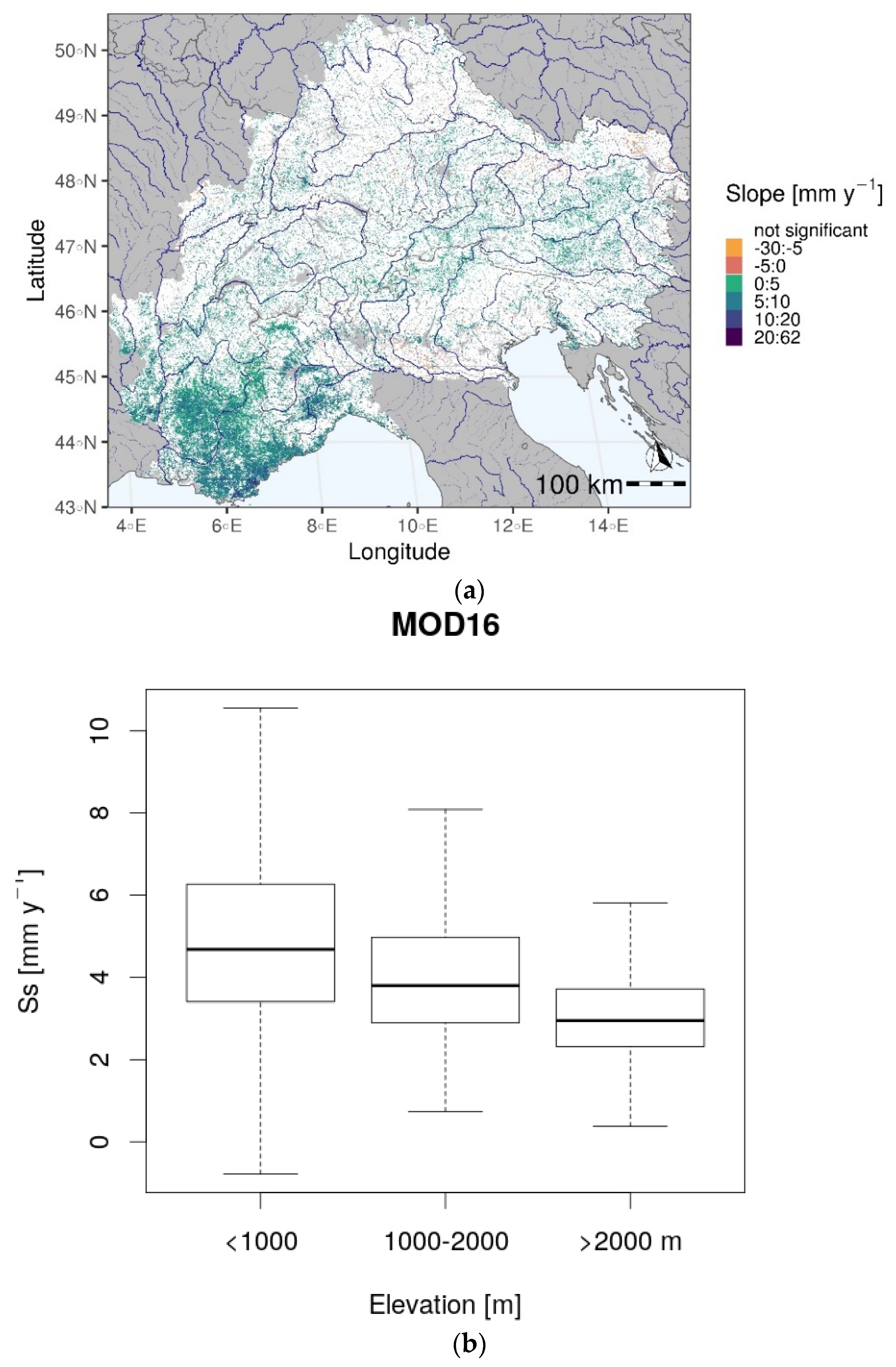
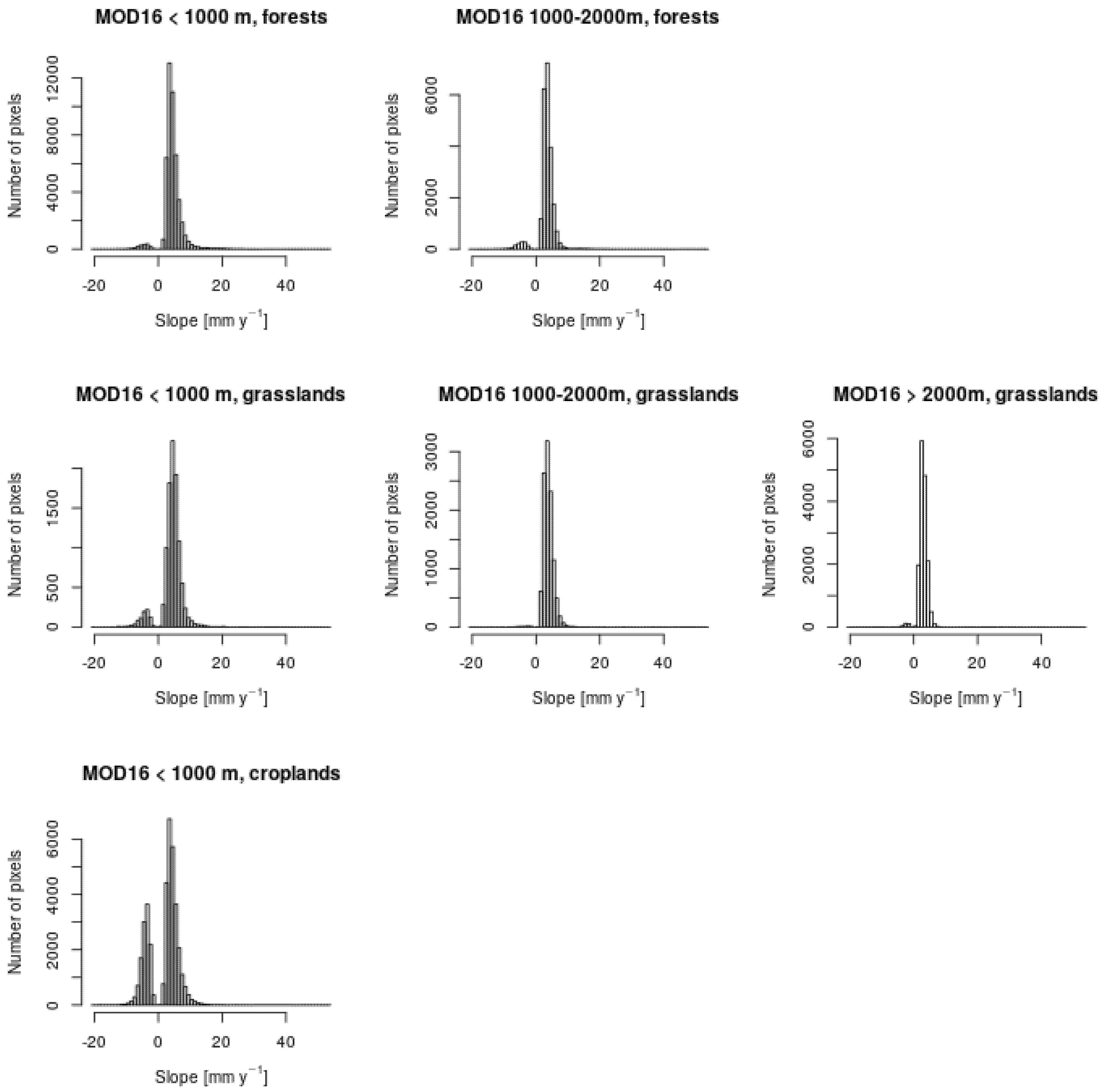
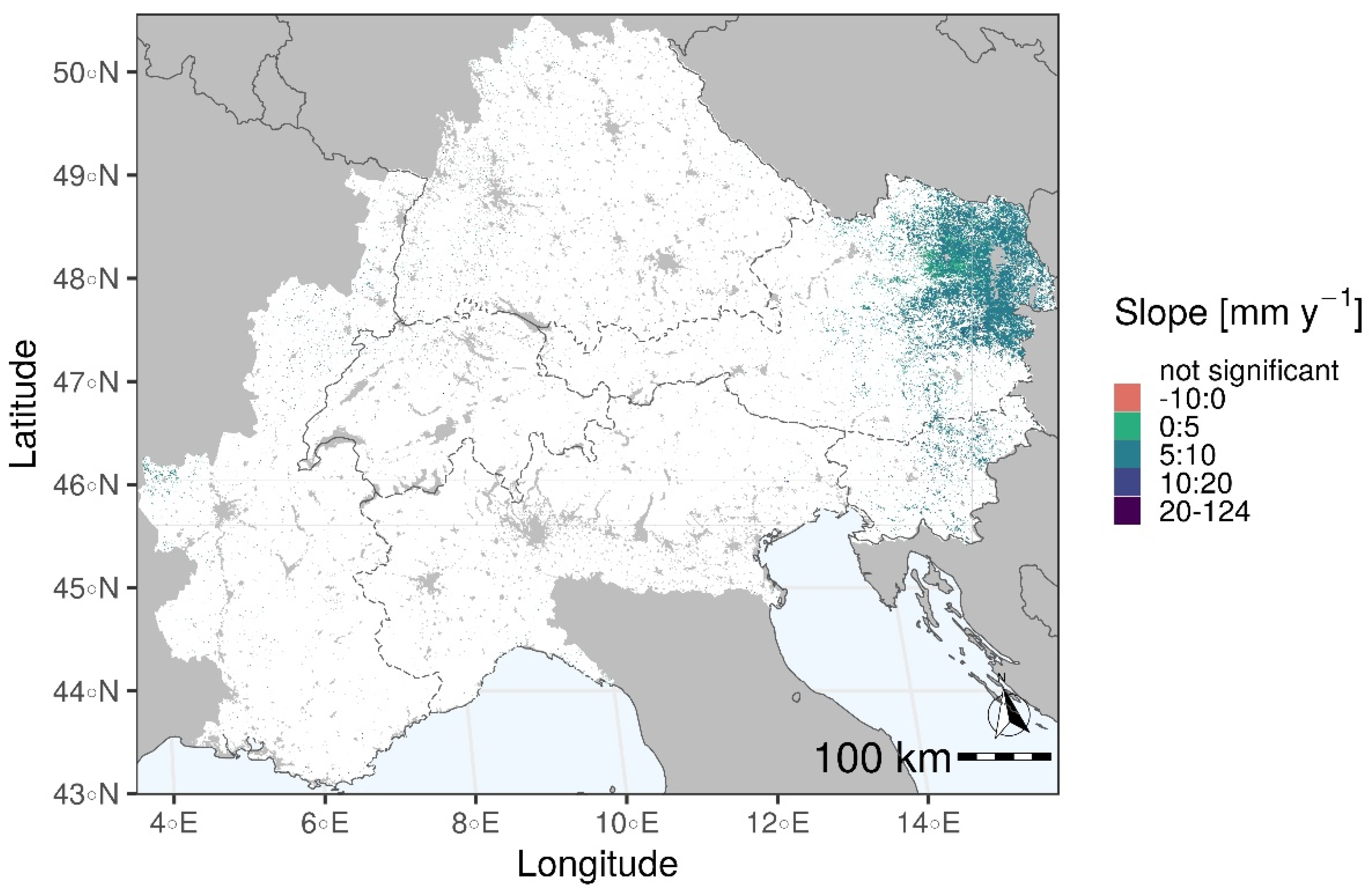
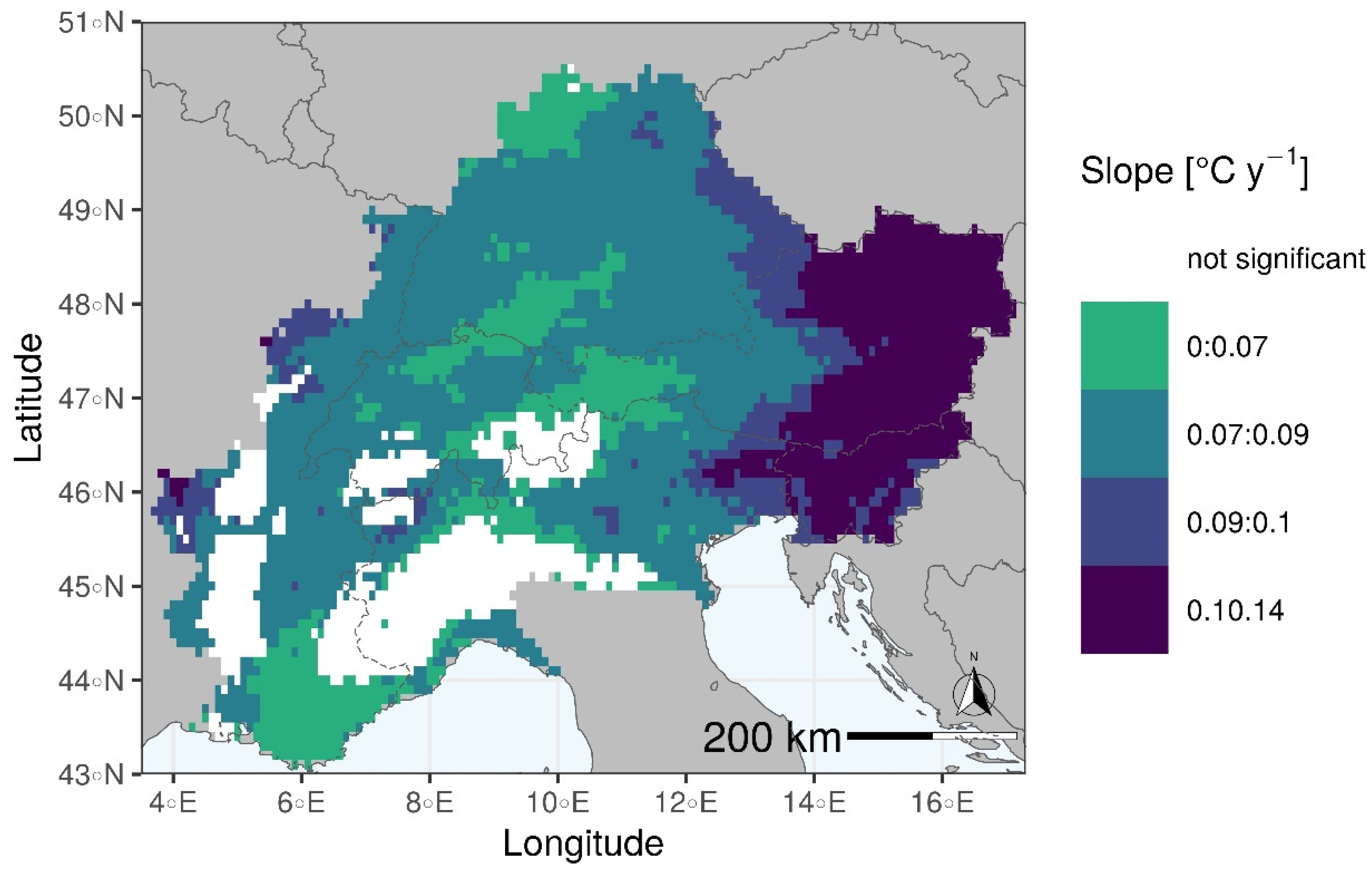
For MOD16, the yearly analysis at pixel level showed extensive significant positive trends all over the Alps, especially pronounced in the south-west, specifically in the catchments of the Durance, Tanaro, Rhone, and Rhine; in the center, in the catchment of the Isar, Inn, and Adige; and in the east, in the catchments of the Donau, Mur, Drau, and Sava (Figure 1). Considering the area of the Alps, 16.6% of it showed an increase in ET, while 1.2% of it showed a decrease. Negative trends were detected in the south, in the Po catchment, and in the north-east, in the Danube catchment. The slope of the trend, on average, decreased with elevation. Most of the areas with a significant positive or negative trend were concentrated at low elevations, especially for grasslands and croplands (Figure 2).

Figure 1.
Sen’s slope of the trend at 5% significance level for yearly ET from the MOD16 product (a); boxplot of the distribution of the slope (Ss) with elevation (b). The period of investigation is 2003–2019.

Figure 2.
Histograms representing the distribution, within the land cover and elevation classes indicated in the titles, of the Sen’s slope of the trend of MOD16 yearly ET at 5% significance level. On the y axis there are 500 m × 500 m pixels.
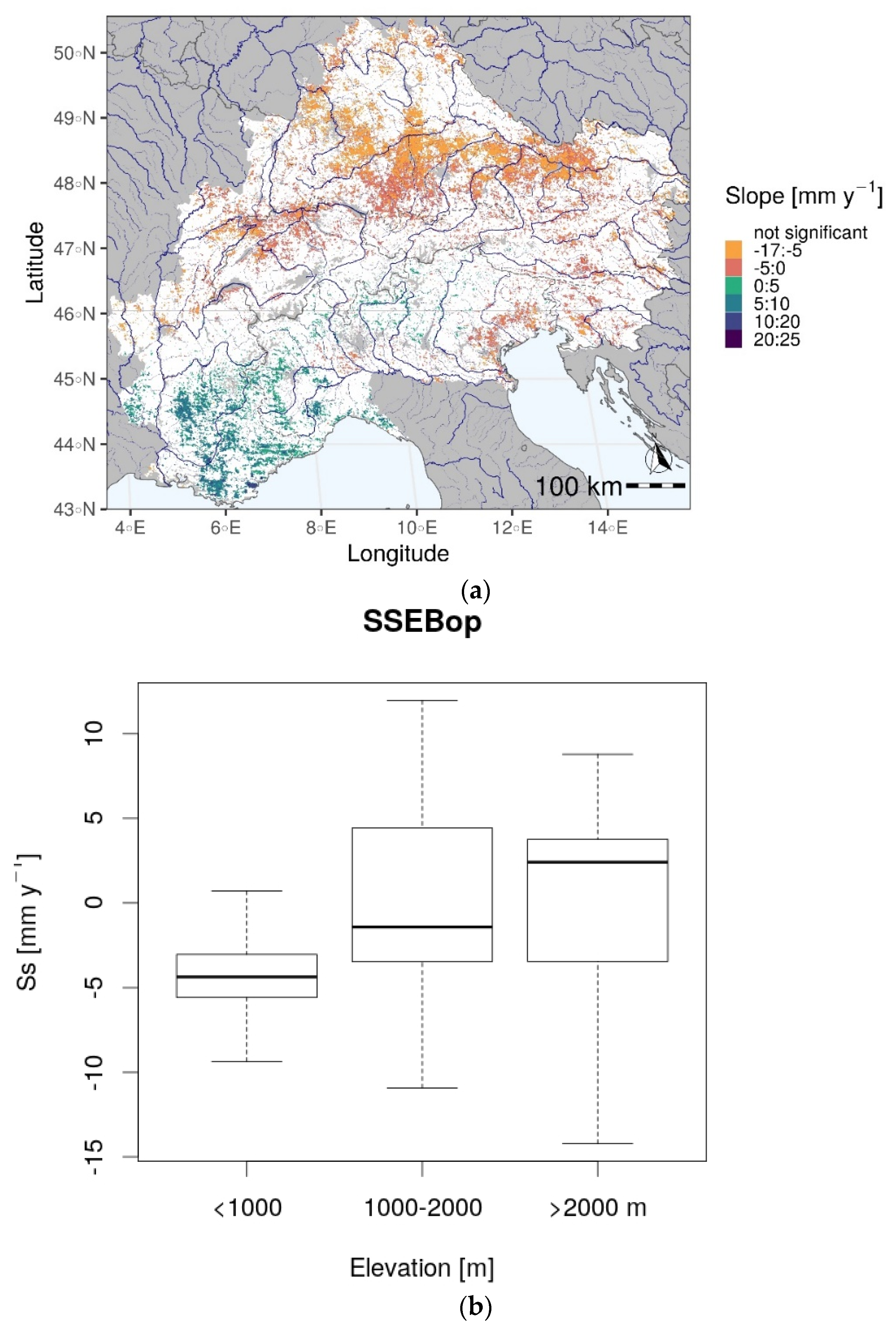
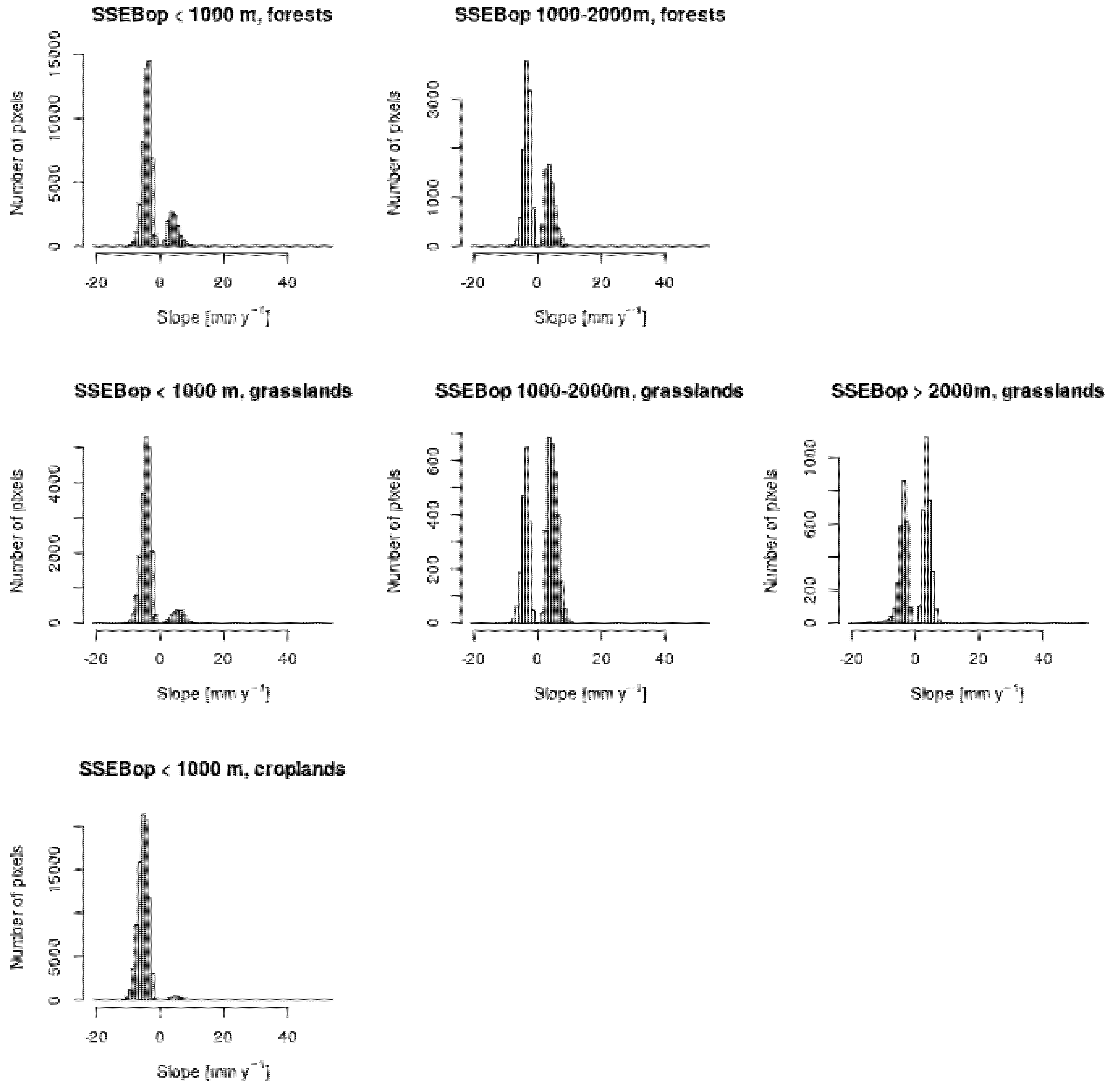
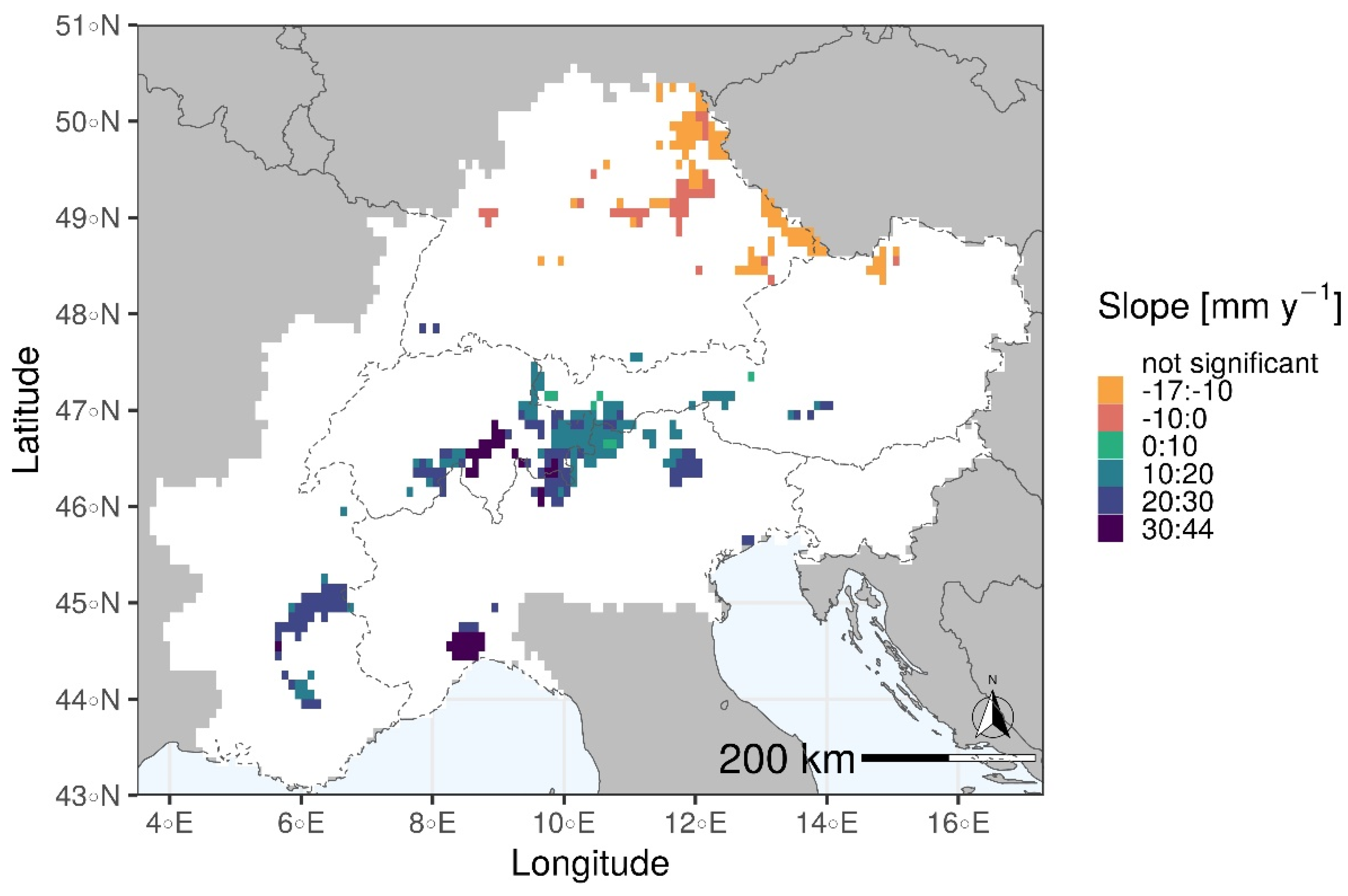
For SSEBop, the results of the trend analysis were different from those obtained from MOD16, with negative trends over most of the Alps, especially in the northern and eastern regions, and there was a positive trend only in the south-west, in the catchments of the Durance, Isere, and Tanaro, as well as in the southern-central Alps, in the catchments of the Adda and Adige (Figure 3). Overall, ET presented a positive trend of over 3.9% of the area of the Alps, and a negative trend over 15.3% of it. The slope of the ET trend was predominantly negative at elevations below 1000 m for all the land cover classes, while it showed a high variability at higher elevations (Figure 4).
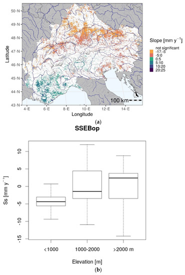
Figure 3.
Sen’s slope of the trend at 5% significance level for yearly ET from the SSEBop product (a); boxplot of the distribution of the slope (Ss) with elevation (b). The period of investigation is 2003–2019.
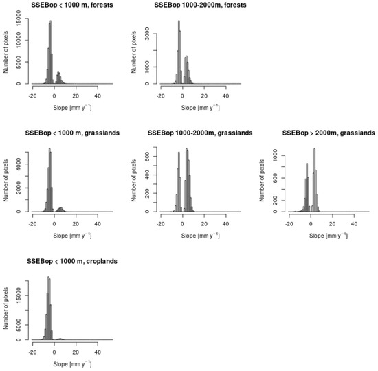
Figure 4.
Histograms representing the distribution, within the land cover and elevation classes indicated in the titles, of the Sen’s slope of the trend of SSEBop yearly ET at 5% significance level. On the y axis there are 500 m × 500 m pixels.
5.3.2. Monthly Analysis
For MOD16, trends in spatially distributed monthly ET were mostly positive for the entire growing season, except for April, while for SSEBop they were mostly negative from July to October, and equally distributed between positive and negative from April to June (Table 5).

Table 5.
Percentage of the area of the Alps with positive and negative slope of the trend (at 5% significance level) in monthly ET for MOD16 and SSEBop, in monthly PET, and in monthly tp.
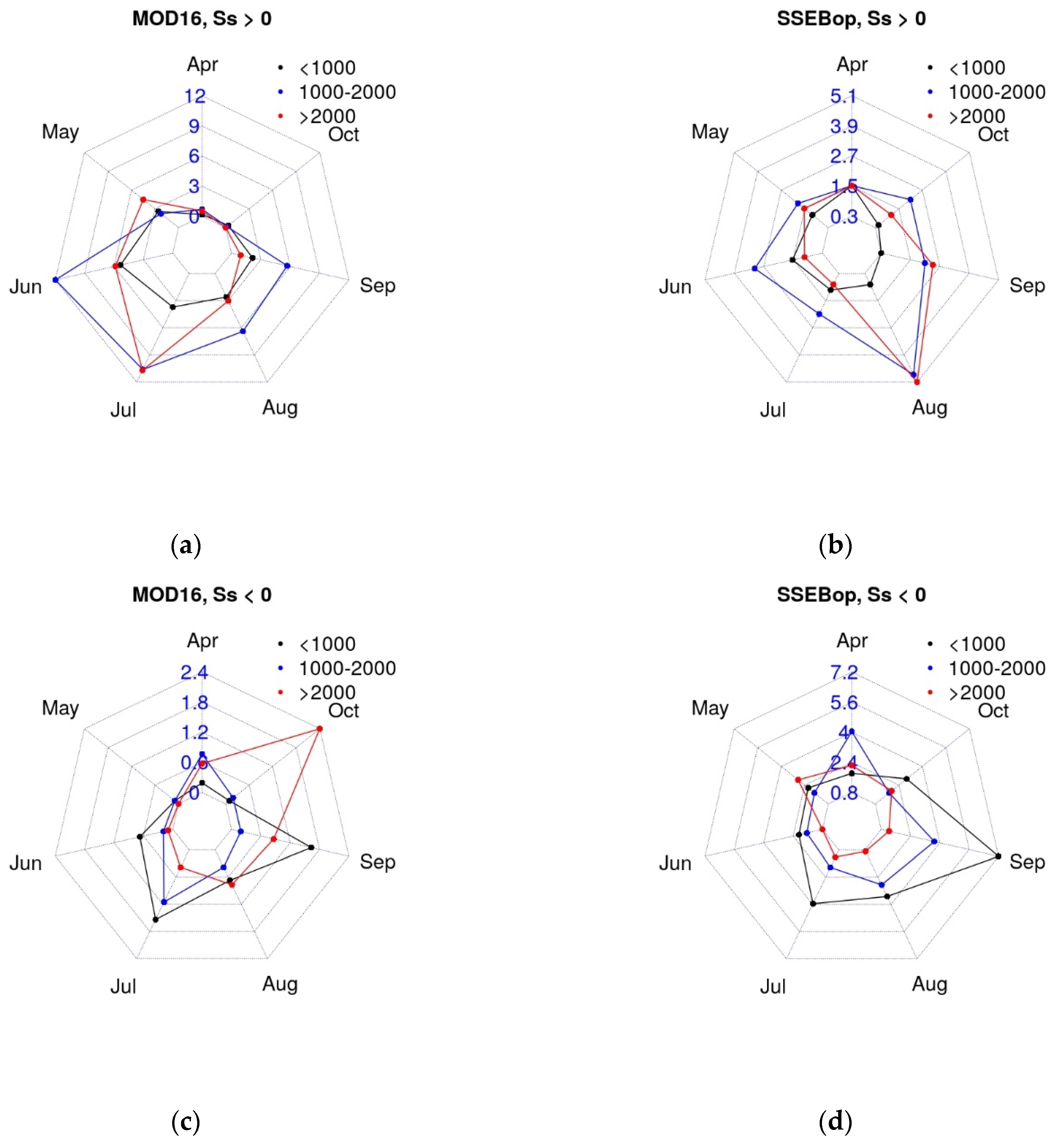
When data were aggregated in elevation ranges (<1000 m, 1000–2000 m, >2000 m), MOD16 trends were mainly positive from May to September, at any elevation, while for SSEBop they showed a high variability, being mostly negative in summer below 1000 m, positive in August above 1000 m, and negative in April and September between 1000 and 2000 m (Figure 5).
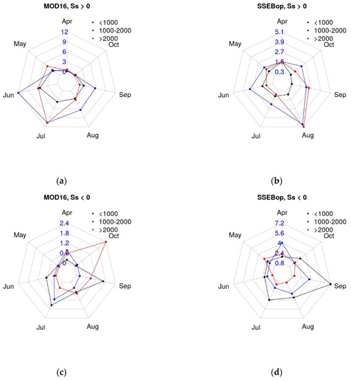
Figure 5.
Percentage of area (blue numbers) in each elevation range with a positive (a,b) or negative (c,d) slope of the trend (Ss) of monthly ET from MOD16 and SSEBop, at 5% significance level. Black, blue, and red lines represent the three elevation classes.
The aggregation by land cover and altitude showed that, for MOD16, trends were positive in May (Supplementary Figure S26) and mainly positive in June, but partially negative for croplands at low elevations (Supplementary Figure S27), mainly positive for forests at any elevation and for grasslands above 1000 m, partially positive and partially negative for low elevation grasslands, mostly negative for croplands below 1000 m from July to September (Supplementary Figures S28–S30), and very low in October (Supplementary Figure S31). For SSEBop, trends in ET were partially positive and partially negative at any elevation and for any land cover in April (Supplementary Figure S32), mostly negative at low elevation for any land cover but partially positive above 1000 m in May (Supplementary Figure S33), partially positive and partially negative for forests, mostly negative for grasslands and croplands at low elevation, mostly positive for high altitude grasslands in June (Supplementary Figure S34), mostly negative at low elevation for any land cover, partially positive and partially negative above 1000 m from July to September (Supplementary Figures S35–S37), and very low and mostly negative for any land cover and elevation in October (Supplementary Figure S38).
5.4. Trend Test and Analysis of Sensitivity for PET
5.4.1. Yearly Analysis
Trends of yearly total PET presented different spatial patterns from the ones of ET, with positive trends observed over 5.4% of the area of the Alps, mainly along the eastern border of the Alpine region, in Austria and Slovenia. Negative trends were found over small areas all over the domain (less than 0.1% of the area of the Alps) (Figure 6).

Figure 6.
Sen’s slope of the trend at 5% significance level for yearly PET. The period of investigation is 2003–2019.
For both MOD16 and SSEBop, the intersection between ET and PET trends exhibited a grouping of data in two clusters, the first with ET and PET trends being both positive, the second with positive PET trends and negative ET trends. To calculate the sensitivity of ET trends compared to PET tends by Equation (7), a linear regression analysis was performed separately within each cluster.
For MOD16, the correlation in the first cluster was moderate (r2 = 0.26, p < 0.001, Supplementary Figure S39), and the sensitivity analysis suggested that, on average, PET trends could be accountable for 1.38 (mm year−1) of the average positive ET trend. In the second cluster, there was no correlation (Supplementary Figure S40). Table 6 also indicates the uncertainties of the estimated sensitivity (s) and impact ().

Table 6.
Correlation and sensitivity analysis between ET trend and the trend of the predictors Vari, including PET, LAI, tp, Ta, and LST. The spatial extent of the area that originated these results is expressed as percentage of the area with a positive or negative ET trend (% area), and of the total area of the Alps (% Alps). s and are the slope of the linear regression and the average impact of the trend of a predictor on the trend of ET, with their respective uncertainties. tET_M and tET_S indicate the trend in ET from MOD16 (tET_M) and SSEBop (tET_S). tTa_GS indicates the trend in air temperature cumulated over the growing season. p-value < 0.001 for all the estimated correlation coefficients. Results were omitted if r2 < 0.01.
For SSEBop, there was no correlation between positive ET trends and positive PET (Supplementary Figure S39). In addition, the correlation between negative ET trends and positive PET trends was very low (r2 = 0.02, p < 0.001) (Supplementary Figure S40, Table 6).
5.4.2. Monthly Analysis
Positive trends in monthly PET were observed mainly from June to August. Negative trends were detected only over very small areas (Table 5). Consequently, the correlation analysis with trends in monthly ET was performed only considering positive PET trends in summer (Table 7).

Table 7.
Monthly correlation and sensitivity analysis between PET and ET trends. The spatial extent of the area that originated these results is expressed as a percentage of the area with positive or negative ET trends (% area). s and are the slope of the linear regression and the average impact of the trend of PET on the trend of ET, with their respective uncertainties. p-value < 0.001 for all the estimated correlation coefficients.
For both MOD16 and SSEBop, ET and PET trends turned out to be aggregated in two clusters, the first with positive ET and PET trends, the second with positive PET trends and negative ET trends. In June, there was correlation only for the second cluster, for both MOD16 and SSEBop, but the coefficient of determination was very low. In July, for MOD16 there was correlation in the first cluster with a positive impact. In contrast, for SSEBop there was correlation in the second cluster, with an estimated positive impact. In August there was correlation only for MOD16, with a positive impact, in both clusters.
5.5. Trend Test and Analysis of Sensitivity for LAI
LAI cumulated over the growing season showed positive trends over 19.5% of the area of the Alps, and negative trends over 0.7% of this area. Positive trends were observed all over the Alps, especially in the southern regions, in France and Italy (Figure 7).
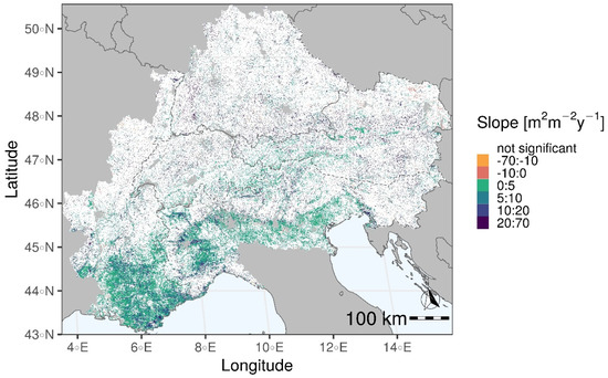
Figure 7.
Sen’s slope of the trend at 5% significance level for LAI cumulated over the growing season. The period of investigation is 2003–2019.
The intersection between ET and LAI trends revealed two main clusters of data, the first with both positive and the second with both negative ET and LAI trends (Table 6).
For MOD16, in the first cluster, covering 50.9% of the area with positive ET trends, the correlation was very low (r2 = 0.06, p < 0.001) (Figure S39), while in the second cluster, covering 17.3% of the area with negative ET trends, it was slightly higher (r2 = 0.14, p < 0.001) (Supplementary Figure S40). The analysis of contribution indicated that, on average, (i) LAI increase could be responsible for 0.15 (mm year−1) of the positive ET trend, and (ii) LAI decrease could be responsible for 0.19 (mm year−1) of the negative ET trend.
For SSEBop, in the first cluster, covering 51.1% of the area with positive ET trends, there was no correlation (r2 = 0.01) (Supplementary Figure S39), and in the second cluster, covering 1.2% of the area with negative ET trends, there was a very low correlation (r2 = 0.05) (Supplementary Figure S40). The estimated sensitivity of ET trends to LAI trends was also very low, and not very meaningful given the low correlation (Table 6).
5.6. Trend Test and Analysis of Sensitivity for Precipitation, tp
5.6.1. Yearly Analysis
Significant trends in yearly precipitation, tp, were found over 7% of the Alpine area, of which 34% had a negative trend and 66% had a positive trend (Figure 8).
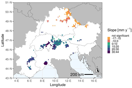
Figure 8.
Sen’s slope of the trend, from 2003 to 2019, at 5% significance level, for yearly total precipitation, tp, from the MSWEP dataset.
The intersection between tp and ET trends allowed identification of two main clusters, the first with positive trends of tp and ET, and the second with negative trends.
For MOD16, the first cluster covered 6.3% of the area with positive ET trends and showed a low correlation (r2 = 0.09) (Supplementary Figure S39). In the second cluster, covering 3.6% of the area with negative ET trends, there was no correlation (Supplementary Figure S40).
For SSEBop, in the first cluster, covering 10.9% of the area with positive ET trends, there was no correlation (Supplementary Figure S39). In the second, with over 4.7% of the area with negative ET trends, there was a low correlation (r2 = 0.10) (Supplementary Figure S40).
5.6.2. Monthly Analysis
On a monthly basis, significant positive trends were found in May, June, July, and October, respectively over 2.8%, 1.2%, 4.2%, and 5.4% of the Alpine area. Negative trends were found in August and September over 15.7% and 3.1% of the Alpine area (Table 5). These trends were correlated with monthly ET trends on which they could have an influence, i.e., in the same and in the following two months.
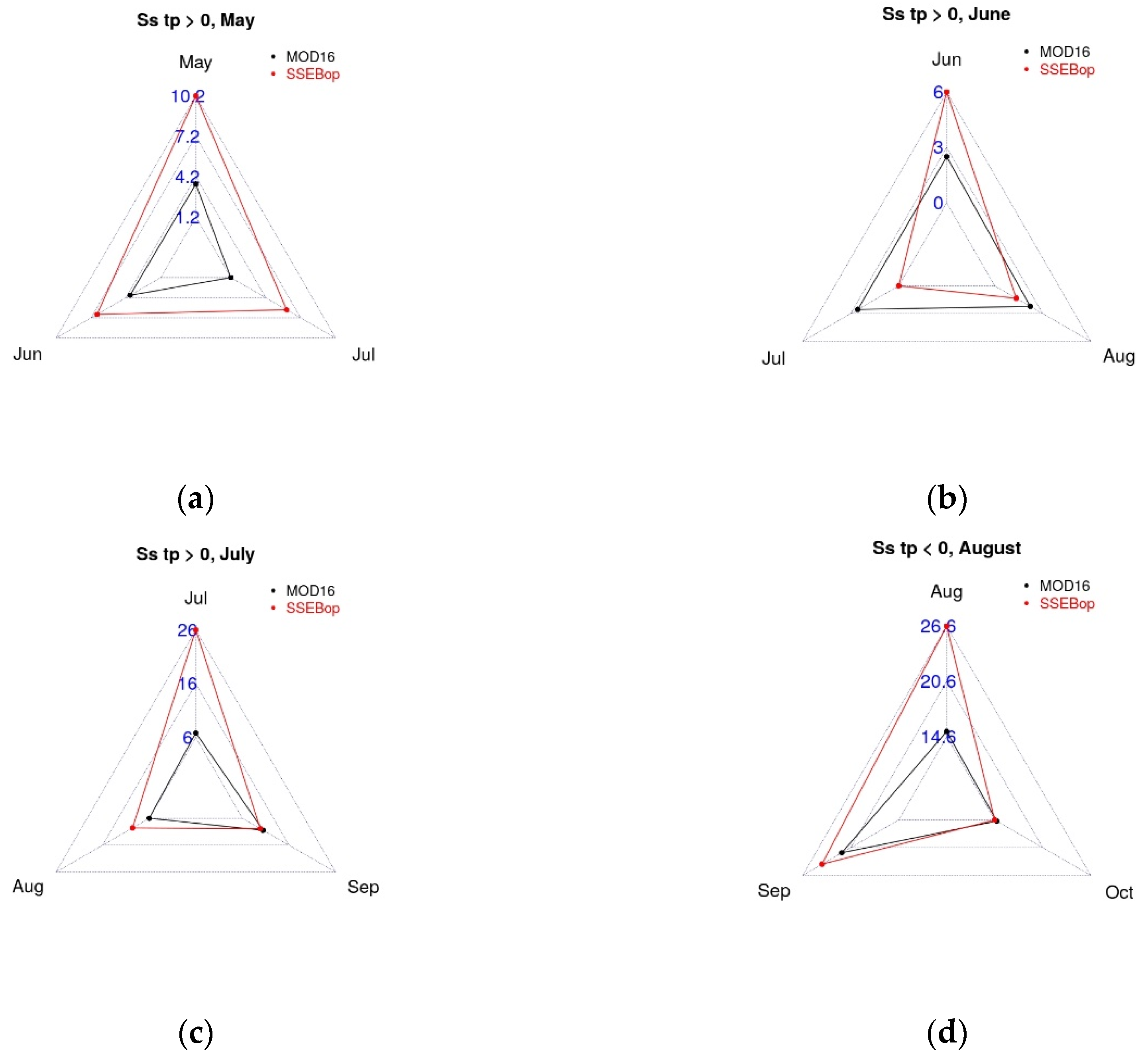
For both MOD16 and SSEBop, there was overlapping between positive tp and ET trends, as well as between negative tp and ET trends (Figure 9). However, the correlation was always extremely low.
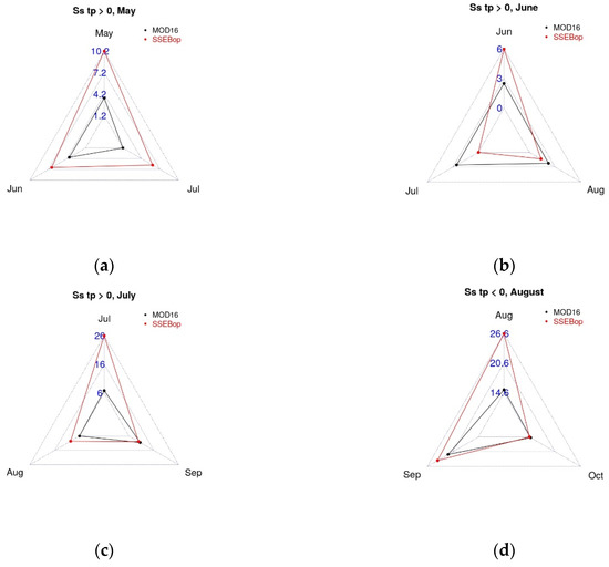
Figure 9.
Area of overlapping between positive monthly tp trends in May, June, and July and positive monthly ET trends in the same and in the following two months (a–c), and between negative monthly tp trends in August and negative monthly ET trends in August, September, and October (d). Areas are expressed as percentage of the area with positive and negative ET trends (blue numbers).
5.7. Trend Test and Analysis of Sensitivity for Air Temperature, Ta
Positive trends were observed in the growing season average air temperature, Ta, all over the Alps, which was up to 0.14 (°C year−1) for the growing season (Figure 10).

Figure 10.
Sen’s slope of the trend at 5% significance level for yearly air temperature, Ta, based on yearly average from March to October, from 2003 to 2019.
For both MOD16 and SSEBop, there was widespread spatial overlapping between Ta and ET trends, and data were clustered in two sets, one with positive trends, over most of the areas with positive ET trends (>70%), the other with positive Ta trends and negative ET trends, over most of the area with negative ET trends (>84%) (Table 6). However, the correlation was very low (Supplementary Figures S39 and S40).
5.8. Trend Test and Analysis of Sensitivity for Land Surface Temperature, LST
Positive trends were observed for growing season average LST over 48% of the Alpine area, up to 0.34 (°C year−1) (Figure 11). Two main data clusters emerged, one with positive LST and ET trends, the other with positive LST and negative ET trends.
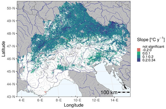
Figure 11.
Sen’s slope of the trend at 5% significance level for yearly land surface temperature, LST, based on yearly average from March to October, from 2003 to 2019.
For MOD16, the first cluster extended over 30% of the area with positive ET trends, and the second covered 77.8% of the area with negative ET trends. No correlation was found (r2 < 0.01) (Supplementary Figures S39 and S40).
For SSEBop, the first cluster covered 70.6% of the area with positive ET trends, while the second extended over 98.5% of the area with negative ET trends. There was correlation only in the second cluster (Supplementary Figure S40), with r2 = 0.15, and the sensitivity analysis indicated that the observed average increase in LST can be related to a decrease in ET of 0.49 (mm year−1).
5.9. Analysis of the Impact of Land Cover and Altitude
The analysis of sensitivity of ET trends to trends in LAI, tp, Ta, and LST was performed separately in combined classes of land cover and altitude.
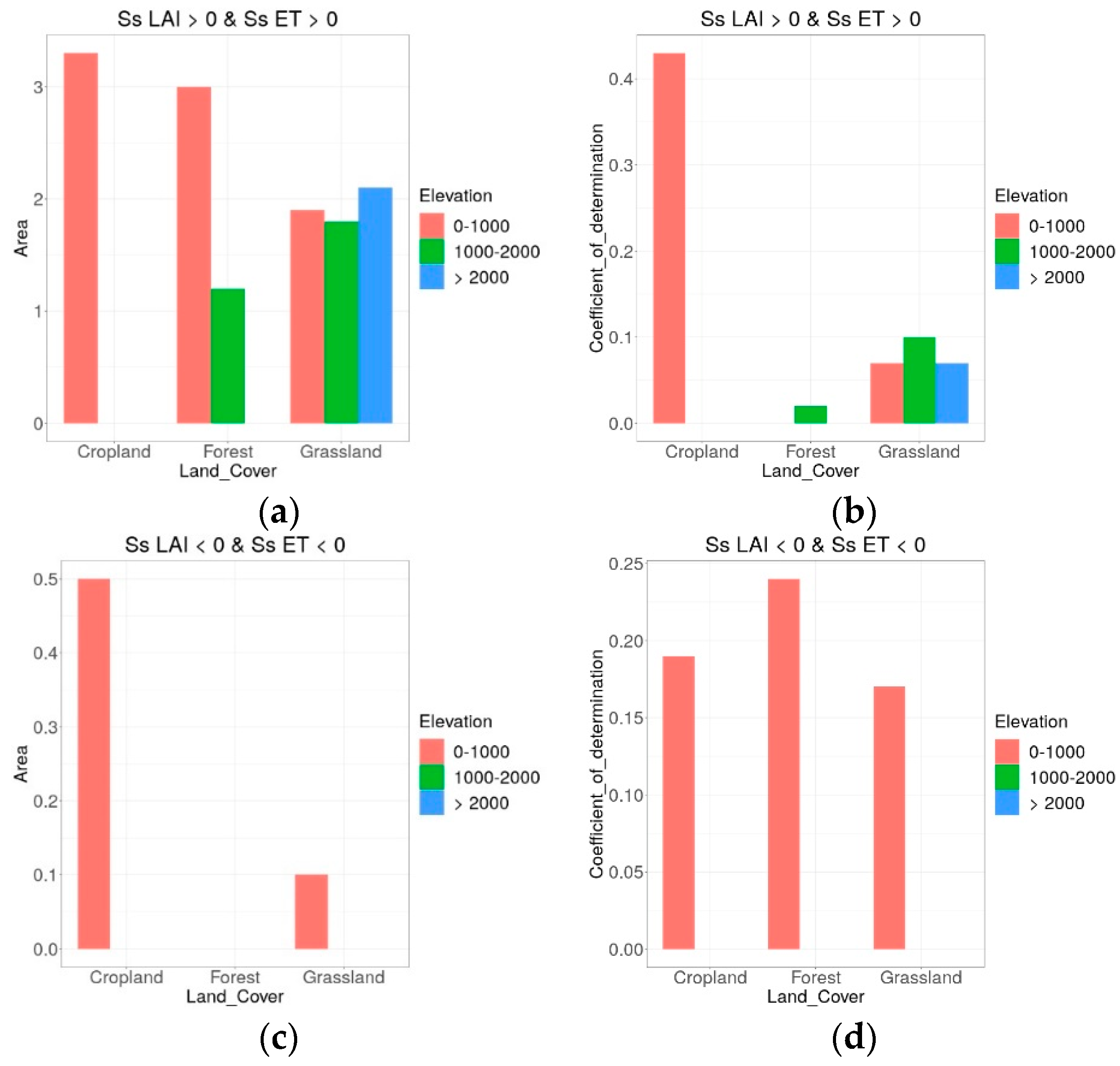
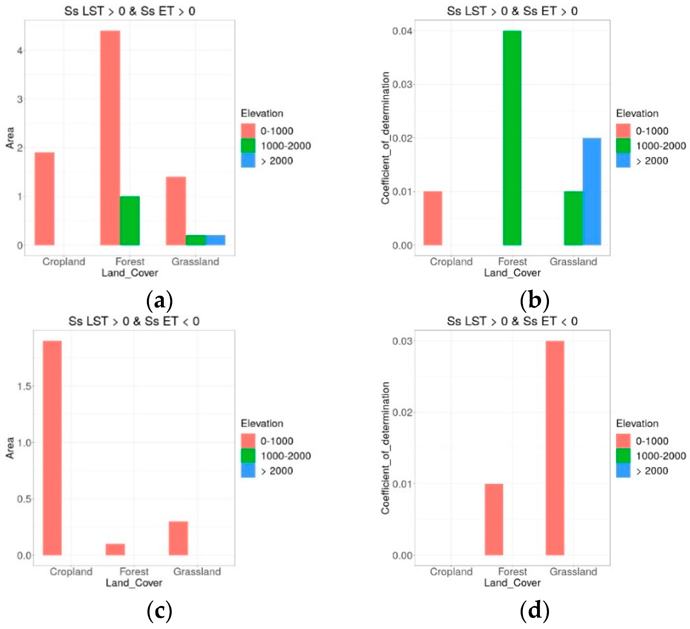
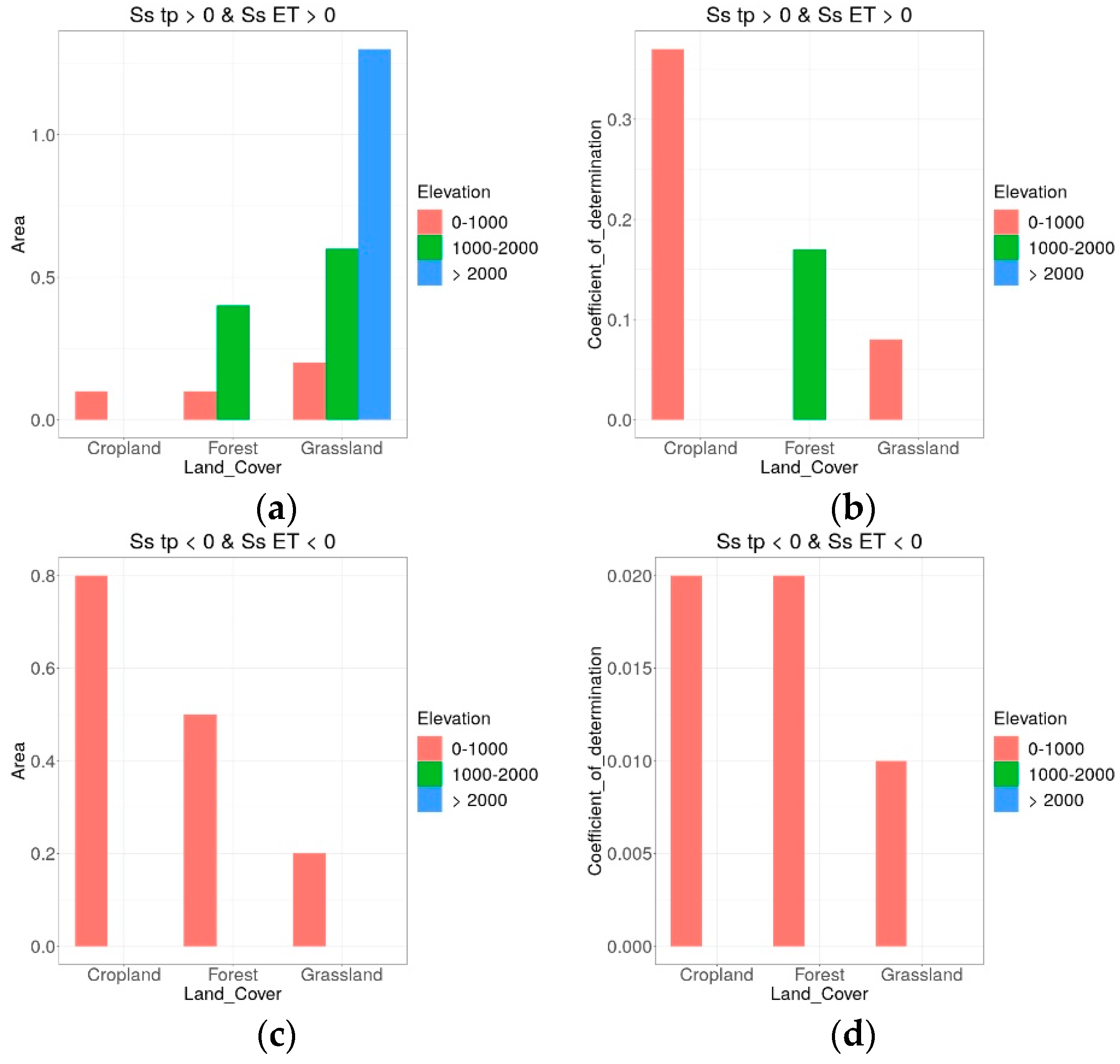
For MOD16, there was a high correlation over a wide area between positive LAI and ET trends for cropland below 1000 m (Figure 12). Grasslands at any altitude also showed significant overlapping between LAI and ET trends, and a moderate correlation. For croplands, there was more overlapping and higher correlation with respect to the other classes for both positive and negative ET and LAI trends. Positive tp trends corresponded to positive ET trends, mainly for forests and grasslands. However, r2 exceeded 0.1 only for forests between 1000 and 2000 m of elevation (Figure 13). All the classes showed an intersection between positive Ta and ET trends, but the correlation was very low (Figure 14). For LST, all the land cover classes at any elevation presented a correspondence between positive LST and ET trends, but low correlations (Figure 15). Negative ET trends corresponded to an increase in LST, mainly over croplands, but with no correlation between the trends.

Figure 12.
Percentage of area in each land cover class where LAI and MOD16 ET trends overlap, per elevation (a,c) and corresponding r2 (b,d). The combination of positive or negative ET and LAI trends is indicated in the title of each plot. “Area” on the y axis is the percentage of the total area within a specific land cover class. Ss is the Sen’s slope of the trend at 5% significance from 2003 to 2019.
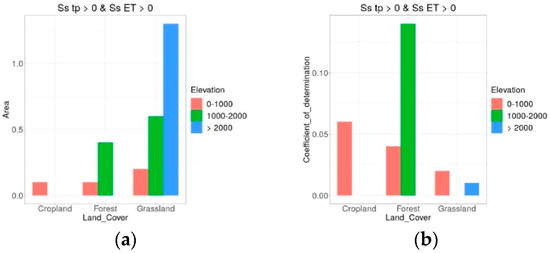
Figure 13.
Percentage of area in each land cover class where tp and MOD16 ET trends overlap, per elevation (a) and corresponding r2 (b). The combination of positive or negative ET and tp trends is indicated in the title of each plot. “Area” on the y axis is the percentage of the total area within each land cover class. Ss is the Sen’s slope of the trend at 5% significance from 2003 to 2019.
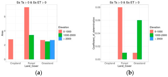
Figure 14.
Percentage of area in each land cover class where Ta and MOD16 ET trends overlap, per elevation (a) and corresponding r2 (b). The combination of positive or negative ET and Ta trends is indicated in the title of each plot. “Area” on the y axis is the percentage of the total area within each land cover class. Ss is the Sen’s slope of the trend at 5% significance from 2003 to 2019.
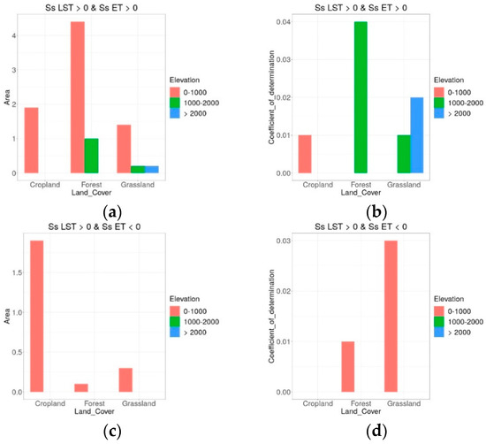
Figure 15.
Percentage of area in each land cover class where LST and MOD16 ET trends overlap, per elevation (a,c) and corresponding r2 (b,d). The combination of positive or negative ET and LST trends is indicated in the title of each plot. “Area” on the y axis is the percentage of the total area within each land cover class. Ss is the Sen’s slope of the trend at 5% significance from 2003 to 2019.
For SSEBop, small areas showed correspondence between positive LAI and ET trends in all the land cover-altitude classes, with very low correlation (Figure 16). Areas with negative LAI and ET trends were found only for croplands and grasslands at low elevations and showed very low correlation. Positive tp trends corresponded to positive ET trends over small regions, especially for grassland and forests, with moderate-low correlations (Figure 17). Negative tp and ET trends overlapped at low elevation, especially for croplands, with very low correlation. Increasing Ta corresponded to increasing ET for all three land cover classes, especially for forest, with low-moderate correlations (Figure 18). Increasing LST corresponded to a decrease in ET for large areas, mainly at low elevations, with moderate-low correlation (Figure 19).
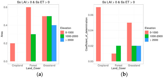
Figure 16.
Percentage of area in each land cover class where LAI and SSEBop ET trends overlap, per elevation (a) and corresponding r2 (b). The combination of positive or negative ET and LAI trends is indicated in the title of each plot. “Area” on the y axis is the percentage of the total area within each land cover class. Ss is the Sen’s slope of the trend at 5% significance from 2003 to 2019.

Figure 17.
Percentage of area in each land cover class where tp and SSEBop ET trends overlap, per elevation (a,c) and corresponding r2 (b,d). The combination of positive or negative ET and tp trends is indicated in the title of each plot. “Area” on the y axis is the percentage of the total area within each land cover class. Ss is the Sen’s slope of the trend at 5% significance from 2003 to 2019.
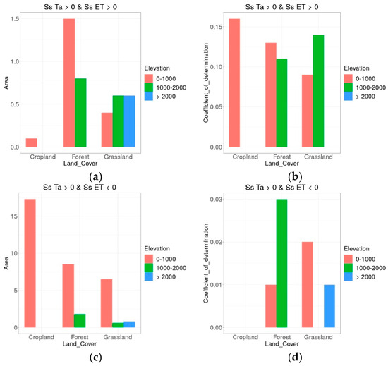
Figure 18.
Percentage of area in each land cover class where Ta and SSEBop ET trends overlap, per elevation (a,c) and corresponding r2 (b,d). The combination of positive or negative ET and Ta trends is indicated in the title of each plot. “Area” on the y axis is the percentage of the total area within each land cover class. Ss is the Sen’s slope of the trend at 5% significance from 2003 to 2019.
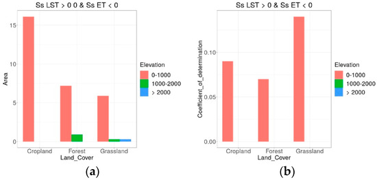
Figure 19.
Percentage of area in each land cover class where LST and SSEBop ET trends overlap, per elevation (a) and corresponding r2 (b). The combination of positive or negative ET and LST trends is indicated in the title of each plot. “Area” on the y axis is the percentage of the total area within each land cover class. Ss is the Sen’s slope of the trend at 5% significance from 2003 to 2019.
6. Discussion
The comparison with latent heat flux measured at eddy flux towers suggested that the two globally available ET products, MOD16 and SSEBop, both based on MODIS satellite data, perform similarly in the Alps. In contrast to studies indicating that SSEBop is generally more reliable than MOD16 [25], MOD16 exhibited a slightly better agreement with observed data in terms of mean daily RMSE and MBD, probably because the spatial resolution plays a crucial role in heterogenous mountain regions. It is reasonable to assume that a MOD16 spatial resolution of 500 m captures the heterogeneity of Alpine vegetation better than the SSEBop spatial resolution of 1 km. However, for both ET products, RMSE values at Alpine eddy flux towers were always close to the upper limit of those found by comparable validation studies over other regions of the world [29,84].
Notably, the correlation analysis at site level did not show major conformity with one of the two satellite-based ET products. On the contrary, the correlation with climate data (Ta, tp, and PET) was more coherent with MOD16 for grasslands, and with SSEBop for forests. In addition, the correlation with LST was consistent with MOD16, while the correlation with LAI was consistent with SSEBop. Because LST is a main input for SSEBop and LAI is a main input for MOD16, the latter result suggests that, in the Alps, both algorithms fail to represent the actual dependence of ET on LAI and LST.
In terms of trends, both MOD16 and SSEBop ET indicated that summer as well as yearly ET increased in the south-west, especially at high-elevation grasslands and forests, and decreased in the south and in the north-east, especially at low elevation croplands and grasslands. However, for MOD16 areas with positive ET, trends prevailed at any elevation, while for SSEBop, areas with negative trends dominated. This divergence might be caused by several differences between the two considered ET products, i.e.,:
- The retrieval algorithms. Both algorithms are based on the Penman–Monteith equation, but MOD16 exploits vapor pressure deficit from climate reanalysis to regulate surface conductance, whereas SSEBop uses the standardized version of the Penman–Monteith equation [85] and calibrates model parameters based on land surface properties derived from satellite data (see point 3 for more details).
- Climate data. Both algorithms use low resolution climate data. In particular, MOD16 uses the GMAO daily meteorological data [27] (including air temperature, incident photosynthetically active radiation, and specific humidity), with an original spatial resolution of 0.5° × 0.6°, spatially smoothed at MODIS pixel level [86]. SSEBop, in contrast, derives climatological daily maximum air temperature from WorldClim [87] (https://www.worldclim.org/data/index.html, accessed on 20 September 2021) and reference evapotranspiration from the daily Global Data Assimilation System (GDAS) dataset [88] (https://www.ncei.noaa.gov/products/weather-climate-models/global-data-assimilation, accessed on 20 September 2021) at a resolution of 100 km, downscaled at 10 km based on the IWMI climatological PET. For SSEBop, the assumption of a static cold boundary derived from climatological air temperature could have an impact on the trends because changes in air temperature are neglected in the estimation of the evaporative fraction.
- Land cover. Both algorithms make strong assumptions regarding the influence of land cover on ET. MOD16 exploits a MODIS-based land cover classification to define biome specific physiological parameters regulating surface conductance to transpiration. These parameters are considered constant over space and time [86], independent of seasonality and geographical region. SSEBop, in contrast, does not explicitly include any land cover classification, but it does exploit land surface characteristics for model parameterizations. Specifically, LST is used to calculate the evaporative fraction, which is regulated by the difference between the observed land surface temperature and the temperature at the cold/wet boundary [24]. The Normalized Vegetation Index (NDVI) is used to choose the cold/wet pixels used to define the conversion coefficient between air temperature and cold boundary temperature. Finally, emissivity and albedo are used to correct low LST values observed over sparsely vegetated surfaces in arid and semi-arid areas.
The trend analysis on environmental drivers of ET changes demonstrated that air temperature and LAI increased all over the Alps, confirming the results of other studies [11,12,39,41,42]. For LAI, few exceptions were found, for example in north-eastern Austria, which is one of the most drought-prone regions in central Europe [89], where precipitation was probably not able to compensate the increasing temperature during the growing season, with consequent impacts on vegetation.
The correlation analysis between ET trends and the trends of the possible drivers indicated that:
- The increase of PET had an impact on the decrease of ET in the eastern Alps, suggesting that this region was particularly subjected to an increase in the atmospheric demand of evaporation.
- Trends in LAI were coincident with trends in ET, but there was correlation only for MOD16. LAI is an input of the MOD16 algorithm. This explains the strong correlation between changes in ET and changes in LAI.
- Trends in LST were coincident with trends in ET, but there was correlation only for SSEBop, likely because LST is one main input of the SSEBop algorithm.
- The correlation between trends in tp and Ta and trends in ET was low. Probably, the correlation analysis on areas aggregated by land cover and elevation could not fully catch the heterogeneity of climate across the Alps. Further analysis based on climatic regions could give more insight into the influence of precipitation and temperature on ET. Regarding Ta, MOD16 and SSEBop are based on global reanalysis with very low spatial resolution, which, in contrast to ERA5_Land [90], do not consider the effect of orography on air temperature. This could cause unrealistic spatial patterns in ET and its trends. For example, at high elevation, temperature is generally the factor limiting vegetation growth and transpiration [91,92]; thus, it is expected that the increase in Ta contributed to the increase in ET. However, for both MOD16 and SSEBop, increasing Ta also matched with increasing ET at low elevation, especially over forests, and only for MOD16 high elevation areas covered by forests and grasslands showed more positive than negative ET trends in correspondence with increasing Ta.
The monthly analysis on the possible impacts of PET and tp on the seasonality of ET trends showed that positive PET trends prevailed in summer, while instead tp increased in May, June, July, and October and decreased in August and September. The effect of PET seems negative in June and diverging between the two ET products in the rest of the summer, while for tp the area of overlapping between positive and negative trends was similar for the two ET products. It can be noticed that changes in the seasonality of tp were much more spread than changes in yearly total tp. However, the correlation with changes in monthly ET was low, and probably, as for the yearly analysis, an aggregation based on climatic regions could provide additional information.
Some limitations affect the analyses presented in this study, specifically:
- The length of the MODIS timeseries might be insufficient to detect long term trends.
- The low resolution of climate reanalysis data might have affected the attribution of spatially distributed changes in ET to Ta. Higher resolution datasets have been developed only for limited regions, e.g., South Tyrol [93] and Switzerland [94,95,96], and it would be desirable that similar attempts are extended to the entire Alpine region in order to support studies regarding feedbacks between changes in climate and in water availability.
- The two MODIS derived ET products considered in the present work rely on modelling assumptions that can be accepted at large scale but might be too strong for the heterogeneous and topographically complex Alpine region. Strong topographic gradients and heterogeneous landcover impact the spatial patterns of ET by influencing the evaporative demand of the atmosphere and canopy conductance. Consequently, despite the unique value of products easily accessible and covering the entire globe, they must be used with care in certain areas, such as mountainous regions, where underlying hypotheses are likely to be violated. Other available products could be explored, such as PML-2 [97] and FluxCom [22], which were not considered in the present study, to not further reduce the length of the timeseries, being available, respectively, from 2002 to 2017 and from 2001 to 2015.
- The impact of climate and land use changes on LAI was not examined in this study. However, a land cover-specific analysis of the factors affecting LAI, and consequently ET, would be important to explain the potential role of biotic and abiotic controls on the Alpine water balance. Nevertheless, long timeseries of accurate LAI, land cover and ET in the Alps, which would be essential for the reliability of such an analysis, are not yet available.
7. Conclusions
This work assessed the applicability of two globally available satellite ET products based on MODIS for detecting trends in the Alps. Although these products have been exploited all around the World (e.g., [98,99,100] for MOD16 and [101,102] for SSEBop), with few studies focusing on mountain regions [103], to the author’s knowledge no study has assessed their accuracy and utility in the Alps, especially with regards to climate change induced shifts in the water cycle.
The results of the trend analysis of MOD16 and SSEBop largely diverged, but they also exhibited some common features, including:
- Positive ET trends in the south-western Alps, both yearly and in the summer months;
- Negative ET trends in the Po valley and in the north-eastern Alps, both on yearly basis and in summer;
- Negative ET trends in the northern Alps in September;
- Predominance of positive trends at high elevations in summer over forests and grasslands;
- Predominance of negative trends at low elevations in summer over grasslands and croplands;
- Concurrence between increasing atmospheric evaporative demand and decreasing ET in the north-eastern Alps;
- Concurrence between vegetation greening (increasing LAI) and positive ET trends over any land cover at any elevation, as well as between browning (decreasing LAI) and negative ET trends over croplands and grasslands at low elevations;
- Concurrence between air and surface warming and ET trends, both positive and negative.
- Potential negative impact of increasing PET in June;
- Potential impact of changes in precipitation in summer, mostly positive from May to July and negative in August and September.
The results obtained for both ET datasets, which can thus be considered the most robust outcome of this study, can have important impacts. In particular, the positive ET trends that emerged from MODIS in summer could affect the dynamics of drought in the Alps. In fact, temperature increase and decreasing winter snow fall, in addition to increasing water use for agriculture and hydropower production, are already causing a reduction in Alpine rivers discharge during summer [104,105,106,107]. Increasing ET can reduce groundwater availability and amplify discharge deficit in summer, when snow melt is secondary for runoff production. This is very likely to happen if the drying trend that has been observed in Central Europe [108], with summer precipitation decrease, will persist, as foreseen by the EURO-CORDEX seasonal projections [109,110]. In addition, the negative ET trends that were found from MODIS at low elevations, especially in the Po valley and in the north-eastern Alps, could indicate a decreasing availability of water with impacts on vegetation health and growth.
A follow up of this work could envisage a combined analysis between ET and the other relevant components of the water cycle of the Alps, i.e., precipitation, soil moisture, snow cover, and runoff, in order to extend the findings of short-term hydrological simulations of the indirect feedbacks of climate change on land surface processes, such as the “the drought paradox”, which has been recently studied by ecohydrological simulations in the Alpine region [5].
As stated in Section 6, this study is affected by some limitations, among which are the spatial resolution of satellite and climate data that drive the two considered algorithms. However, as to the MOD16 algorithm, the recent availability of high resolution climate reanalysis [111] and the possibility to retrieve vegetation biophysical properties from Sentinel-2 satellite data [112] open novel possibilities for new implementations of the Penman–Monteith equation, which is less affected by the low resolution of input data. As to the SSEBop algorithm, and in general algorithms that solve the earth’s surface energy budget with different levels of complexity [113,114], they are still limited by the lack of thermal infrared (TIR) data with a proper spatial-temporal resolution. In addition to ongoing efforts in downscaling TIR data by exploiting its dependence on high resolution optical data [115,116], new missions, such as ECOSTRESS [117] and the ESA candidate mission LSTM [118], could help overcoming these limitations and provide more suitable data for future investigations on ET changes in the Alps.
Supplementary Materials
The following are available online at https://www.mdpi.com/article/10.3390/rs13214316/s1. Figure S1: Correlation between growing season average air temperature measured at eddy flux towers sites and extracted from ERA5 Land reanalysis at the location of the tower sites, Figure S2: Correlation between growing season average air temperature measured at eddy flux towers sites and growing season average LST extracted from the MOD11 product at the location of the tower sites, Figure S3: Timeseries of ET from eddy covariance measurements and from the MOD16 product at the Fluxnet site IT-Ren, Figure S4: Timeseries of ET from eddy covariance measurements and from the MOD16 product at the Fluxnet site IT-MBo, Figure S5: Timeseries of ET from eddy covariance measurements and from the MOD16 product at the Fluxnet site IT-LAV, Figure S6: Timeseries of ET from eddy covariance measurements and from the MOD16 product at the Fluxnet site CH-Fru, Figure S7: Timeseries of ET from eddy covariance measurements and from the MOD16 product at the Fluxnet site CH_Dav, Figure S8: Timeseries of ET from eddy covariance measurements and from the MOD16 product at the Fluxnet site CH_Cha, Figure S9: Timeseries of ET from eddy covariance measurements and from the MOD16 product at the Fluxnet site AT_Neu, Figure S10: Timeseries of ET from eddy covariance measurements and from the MOD16 product at the Fluxnet site IT-Tor, Figure S11: Timeseries of ET from eddy covariance measurements and from the SSEBop product at the Fluxnet site IT-Ren, Figure S12: Timeseries of ET from eddy covariance measurements and from the SSEBop product at the Fluxnet site IT-MBo, Figure S13: Timeseries of ET from eddy covariance measurements and from the SSEBop product at the Fluxnet site IT-Lav, Figure S14: Timeseries of ET from eddy covariance measurements and from the SSEBop product at the Fluxnet site CH_Fru, Figure S15: Timeseries of ET from eddy covariance measurements and from the SSEBop product at the Fluxnet site CH_Dav, Figure S16: Timeseries of ET from eddy covariance measurements and from the SSEBop product at the Fluxnet site CH-Cha, Figure S17: Timeseries of ET from eddy covariance measurements and from the SSEBop product at the Fluxnet site AT_Neu, Figure S18: Timeseries of ET from eddy covariance measurements and from the SSEBop product at the Fluxnet site IT-Tor, Figure S19: Pixel-wise correlation and p-value between MOD16 yearly total ET and LAI, LST, PET, tp and Ta. LAI (MODIS), PET (MODIS) and tp (MSWEP) were cumulated over the growing season, while Ta (ERA5-Land) and LST (MODIS) were averaged over the growing season, Figure S20: Pixel-wise correlation and p-value between SSEBop yearly total ET and LAI, LST, PET, tp and Ta. LAI (MODIS), PET (MODIS) and tp (MSWEP) were cumulated over the growing season, while Ta (ERA5-Land) and LST (MODIS) were averaged over the growing season, Figure S21: Distribution of the correlation and p-value between MOD16 and SSEBop ET and MODIS LAI. All the data were aggregated over the growing season and divided in combined classes of land cover and altitude, Figure S22: Distribution of the correlation and p-value between MOD16 and SSEBop ET and MODIS LST. All the data were aggregated over the growing season and divided in combined classes of land cover and altitude, Figure S23: Distribution of the correlation and p-value between MOD16 and SSEBop ET and MODIS PET. All the data were aggregated over the growing season and divided in combined classes of land cover and altitude, Figure S24: Distribution of the correlation and p-value between MOD16 and SSEBop ET and MSWEP precipitation All the data were aggregated over the growing season and divided in combined classes of land cover and altitude, Figure S25: Distribution of the correlation and p-value between MOD16 and SSEBop ET and ERA5-Land air temperature. All the data were aggregated over the growing season and divided in combined classes of land cover and altitude, Figure S26: Distribution with elevation and land cover, in number of 500 m × 500 m pixels, of the Sen’s slope of the trend of MOD16 monthly ET in May, at 5% significance level, Figure S27: Distribution with elevation and land cover, in number of 500 m × 500 m pixels, of the Sen’s slope of the trend of MOD16 monthly ET in June, at 5% significance level, Figure S28: Distribution with elevation and land cover, in number of 500 m × 500 m pixels, of the Sen’s slope of the trend of MOD16 monthly ET in July, at 5% significance level, Figure S29: Distribution with elevation and land cover, in number of 500 m × 500 m pixels, of the Sen’s slope of the trend of MOD16 monthly ET in August, at 5% significance level, Figure S30: Distribution with elevation and land cover, in number of 500 m × 500 m pixels, of the Sen’s slope of the trend of MOD16 monthly ET in September, at 5% significance level, Figure S31: Distribution with elevation and land cover, in number of 500 m × 500 m pixels, of the Sen’s slope of the trend of MOD16 monthly ET in October, at 5% significance level, Figure S32: Distribution with elevation and land cover, in number of 500 m × 500 m pixels, of the Sen’s slope of the trend of SSEBop monthly ET in April, at 5% significance level, Figure S33: Distribution with elevation and land cover, in number of 500 m × 500 m pixels, of the Sen’s slope of the trend of SSEBop monthly ET in May, at 5% significance level, Figure S34: Distribution with elevation and land cover, in number of 500 m × 500 m pixels, of the Sen’s slope of the trend of SSEBop monthly ET in June, at 5% significance level, Figure S35: Distribution with elevation and land cover, in number of 500 m × 500 m pixels, of the Sen’s slope of the trend of SSEBop monthly ET in July, at 5% significance level, Figure S36: Distribution with elevation and land cover, in number of 500 m × 500 m pixels, of the Sen’s slope of the trend of SSEBop monthly ET in August, at 5% significance level, Figure S37: Distribution with elevation and land cover, in number of 500 m × 500 m pixels, of the Sen’s slope of the trend of SSEBop monthly ET in September, at 5% significance level, Figure S38: Distribution with elevation and land cover, in number of 500 m × 500 m pixels, of the Sen’s slope of the trend of SSEBop monthly ET in October, at 5% significance level, Figure S39: Correlation between positive yearly ET trends and trends in PET, LAI, tp, Ta and LST, Figure S40: Correlation between negative yearly ET trends and trends in PET, LAI, tp, Ta and LST, Flowchart.pptx: schematic representation of the Methods section, Stations.html: interactive map indicating the study area and the position and characteristics of eddy covariance stations.
Funding
This study was partially funded by the project ADO, Alpine Drought Observatory, 2019–2022, co-financed by the European Regional Development Fund through the Interreg Alpine Space program. The funding source had no role in the design of this study.
Data Availability Statement
Publicly available datasets were analyzed in this study. These datasets can be found at the following links: https://fluxnet.org/data/fluxnet2015-dataset/ accessed on 29 April 2021 for the FLUXNET2015 dataset, https://edcintl.cr.usgs.gov/downloads/sciweb1/shared/fews/web/global/ accessed on 29 April 2021 for SSEBop ET, https://search.earthdata.nasa.gov/search accessed on 24 August 2021 for the MOD16, MOD15, MCD12, and MOD11 products, https://cds.climate.copernicus.eu/cdsapp#!/dataset/reanalysis-era5-single-levels-monthly-means?tab=form accessed on 29 April 2021 for ERA5-Land reanalysis, and http://www.gloh2o.org/mswep/ accessed on 24 August 2021 for MSWEP precipitation.
Conflicts of Interest
The author declares no conflict of interest.
References
- Oki, T.; Kanae, S. Global hydrological cycles and world water resources. Science 2006, 313, 1068–1072. [Google Scholar] [CrossRef] [PubMed] [Green Version]
- Forzieri, G.; Alkama, R.; Miralles, D.G.; Cescatti, A. Response to Comment on Satellites reveal contrasting responses of regional climate to the widespread greening of Earth. Science 2018, 360, aap9664. [Google Scholar] [CrossRef] [PubMed] [Green Version]
- Boé, J.; Terray, L. Uncertainties in summer evapotranspiration changes over Europe and implications for regional climate change. Geophys. Res. Lett. 2008, 35, 5702. [Google Scholar] [CrossRef] [Green Version]
- Bonan, G.B. Forests and climate change: Forcings, feedbacks, and the climate benefits of forests. Science 2008, 320, 1444–1449. [Google Scholar] [CrossRef] [Green Version]
- Mastrotheodoros, T.; Pappas, C.; Molnar, P.; Burlando, P.; Manoli, G.; Parajka, J.; Rigon, R.; Szeles, B.; Bottazzi, M.; Hadjidoukas, P.; et al. More green and less blue water in the Alps during warmer summers. Nat. Clim. Chang. 2020, 10, 155–161. [Google Scholar] [CrossRef]
- Anderson, M.C.; Zolin, C.A.; Sentelhas, P.C.; Hain, C.R.; Semmens, K.; Tugrul Yilmaz, M.; Gao, F.; Otkin, J.A.; Tetrault, R. The Evaporative Stress Index as an indicator of agricultural drought in Brazil: An assessment based on crop yield impacts. Remote Sens. Environ. 2016, 174, 82–99. [Google Scholar] [CrossRef]
- Bombelli, G.M.; Soncini, A.; Bianchi, A.; Bocchiola, D. Potentially modified hydropower production under climate change in the Italian Alps. Hydrol. Process. 2019, 33, 2355–2372. [Google Scholar] [CrossRef]
- Schulze, E.-D. The Regulation of Plant Transpiration: Interactions of Feedforward, Feedback, and Futile Cycles. In Flux Control in Biological Systems; Elsevier: Amsterdam, The Netherlands, 1994; pp. 203–235. [Google Scholar]
- Yang, Y.; Anderson, M.; Gao, F.; Hain, C.; Noormets, A.; Sun, G.; Wynne, R.; Thomas, V.; Sun, L. Investigating impacts of drought and disturbance on evapotranspiration over a forested landscape in North Carolina, USA using high spatiotemporal resolution remotely sensed data. Remote Sens. Environ. 2020, 238, 111018. [Google Scholar] [CrossRef]
- Hagg, W.; Braun, L. The Influence of Glacier Retreat on Water Yield from High Mountain Areas: Comparison of Alps and Central Asia. In Climate and Hydrology in Mountain Areas; John Wiley & Sons, Ltd.: Hoboken, NJ, USA, 2006; pp. 261–275. ISBN 0470858141. [Google Scholar]
- Zimmermann, N.E.; Gebetsroither, E.; Züger, J.; Schmatz, D.; Psomas, A. Future Climate of the European Alps. In Management Strategies to Adapt Alpine Space Forests to Climate Change Risks; BoD—Books on Demand: Norderstedt, Germany, 2013. [Google Scholar] [CrossRef] [Green Version]
- Rebetez, M.; Reinhard, M. Monthly air temperature trends in Switzerland 1901–2000 and 1975–2004. Theor. Appl. Climatol. 2008, 91, 27–34. [Google Scholar] [CrossRef] [Green Version]
- Notarnicola, C. Hotspots of snow cover changes in global mountain regions over 2000–2018. Remote Sens. Environ. 2020, 243, 111781. [Google Scholar] [CrossRef]
- Viviroli, D.; Archer, D.R.; Buytaert, W.; Fowler, H.J.; Greenwood, G.B.; Hamlet, A.F.; Huang, Y.; Koboltschnig, G.; Litaor, M.I.; López-Moreno, J.I.; et al. Climate change and mountain water resources: Overview and recommendations for research, management and policy. Hydrol. Earth Syst. Sci. 2011, 15, 471–504. [Google Scholar] [CrossRef] [Green Version]
- Stoy, P.C.; Mauder, M.; Foken, T.; Marcolla, B.; Boegh, E.; Ibrom, A.; Arain, M.A.; Arneth, A.; Aurela, M.; Bernhofer, C.; et al. A data-driven analysis of energy balance closure across FLUXNET research sites: The role of landscape scale heterogeneity. Agric. For. Meteorol. 2013, 171–172, 137–152. [Google Scholar] [CrossRef] [Green Version]
- Anderson, M.C.; Kustas, W.P.; Norman, J.M.; Hain, C.R.; Mecikalski, J.R.; Schultz, L.; González-Dugo, M.P.; Cammalleri, C.; D’Urso, G.; Pimstein, A.; et al. Mapping daily evapotranspiration at field to continental scales using geostationary and polar orbiting satellite imagery. Hydrol. Earth Syst. Sci. 2011, 15, 223–239. [Google Scholar] [CrossRef] [Green Version]
- Guzinski, R.; Nieto, H. Evaluating the feasibility of using Sentinel-2 and Sentinel-3 satellites for high-resolution evapotranspiration estimations. Remote Sens. Environ. 2019, 221, 157–172. [Google Scholar] [CrossRef]
- Senay, G.B.; Bohms, S.; Singh, R.K.; Gowda, P.H.; Velpuri, N.M.; Alemu, H.; Verdin, J.P. Operational Evapotranspiration Mapping Using Remote Sensing and Weather Datasets: A New Parameterization for the SSEB Approach. JAWRA J. Am. Water Resour. Assoc. 2013, 49, 577–591. [Google Scholar] [CrossRef] [Green Version]
- Xu, D.; Agee, E.; Wang, J.; Ivanov, V.Y. Estimation of Evapotranspiration of Amazon Rainforest Using the Maximum Entropy Production Method. Geophys. Res. Lett. 2019, 46, 1402–1412. [Google Scholar] [CrossRef]
- Maselli, F.; Papale, D.; Chiesi, M.; Matteucci, G.; Angeli, L.; Raschi, A.; Seufert, G. Operational monitoring of daily evapotranspiration by the combination of MODIS NDVI and ground meteorological data: Application and evaluation in Central Italy. Remote Sens. Environ. 2014, 152, 279–290. [Google Scholar] [CrossRef]
- Caparrini, F.; Castelli, F.; Entekhabi, D. Mapping of land-atmosphere heat fluxes and surface parameters with remote sensing data. Bound.-Lay. Meteorol. 2003, 107, 605–633. [Google Scholar] [CrossRef]
- Jung, M.; Koirala, S.; Weber, U.; Ichii, K.; Gans, F.; Camps-Valls, G.; Papale, D.; Schwalm, C.; Tramontana, G.; Reichstein, M. The FLUXCOM ensemble of global land-atmosphere energy fluxes. Sci. Data 2019, 6, 74. [Google Scholar] [CrossRef] [PubMed] [Green Version]
- Running, S.W.; Mu, Q.; Zhao, M.; Moreno, A. User’s Guide MODIS Global Terrestrial Evapotranspiration (ET) Product (NASA MOD16A2/A3) NASA Earth Observing System MODIS Land Algorithm. 2017. Available online: https://ladsweb.modaps.eosdis.nasa.gov/missions-and-measurements/modis/MOD16_ET_User-Guide_2017.pdf (accessed on 21 October 2021).
- Senay, G.B.; Kagone, S.; Velpuri, N.M. Operational global actual evapotranspiration: Development, evaluation, and dissemination. Sensors 2020, 20, 1915. [Google Scholar] [CrossRef]
- Elnashar, A.; Wang, L.; Wu, B.; Zhu, W.; Zeng, H. Synthesis of global actual evapotranspiration from 1982 to 2019. Earth Syst. Sci. Data 2021, 13, 447–480. [Google Scholar] [CrossRef]
- Velpuri, N.M.; Senay, G.B.; Singh, R.K.; Bohms, S.; Verdin, J.P. A comprehensive evaluation of two MODIS evapotranspiration products over the conterminous United States: Using point and gridded FLUXNET and water balance ET. Remote Sens. Environ. 2013, 139, 35–49. [Google Scholar] [CrossRef]
- Mu, Q.; Zhao, M.; Running, S.W. Improvements to a MODIS global terrestrial evapotranspiration algorithm. Remote Sens. Environ. 2011, 115, 1781–1800. [Google Scholar] [CrossRef]
- Abiodun, O.O.; Guan, H.; Post, V.E.A.; Batelaan, O. Comparison of MODIS and SWAT evapotranspiration over a complex terrain at different spatial scales. Hydrol. Earth Syst. Sci 2018, 22, 2775–2794. [Google Scholar] [CrossRef] [Green Version]
- Ruhoff, A.L.; Paz, A.R.; Aragao, L.E.O.C.; Mu, Q.; Malhi, Y.; Collischonn, W.; Rocha, H.R.; Running, S.W. Assessment of the MODIS global evapotranspiration algorithm using eddy covariance measurements and hydrological modelling in the Rio Grande basin. Hydrol. Sci. J. 2013, 58, 1658–1676. [Google Scholar] [CrossRef]
- Zhang, Y.; Peña-Arancibia, J.L.; McVicar, T.R.; Chiew, F.H.S.; Vaze, J.; Liu, C.; Lu, X.; Zheng, H.; Wang, Y.; Liu, Y.Y.; et al. Multi-decadal trends in global terrestrial evapotranspiration and its components. Sci. Rep. 2016, 6, 19124. [Google Scholar] [CrossRef] [PubMed] [Green Version]
- Hobeichi, S.; Abramowitz, G.; Evans, J. Robust historical evapotranspiration trends across climate regimes. Hydrol. Earth Syst. Sci. Discuss. 2020, 1–32. [Google Scholar] [CrossRef]
- Pan, S.; Pan, N.; Tian, H.; Friedlingstein, P.; Sitch, S.; Shi, H.; Arora, V.K.; Haverd, V.; Jain, A.K.; Kato, E.; et al. Evaluation of global terrestrial evapotranspiration using state-of-the-art approaches in remote sensing, machine learning and land surface modeling. Hydrol. Earth Syst. Sci. 2020, 24, 1485–1509. [Google Scholar] [CrossRef] [Green Version]
- Zhang, K.; Kimball, J.S.; Nemani, R.R.; Running, S.W.; Hong, Y.; Gourley, J.J.; Yu, Z. Vegetation Greening and Climate Change Promote Multidecadal Rises of Global Land Evapotranspiration. Sci. Rep. 2015, 5, 15956. [Google Scholar] [CrossRef]
- Duethmann, D.; Blöschl, G. Why has catchment evaporation increased in the past 40 years? A data-based study in Austria. Hydrol. Earth Syst. Sci 2018, 22, 5143–5158. [Google Scholar] [CrossRef] [Green Version]
- Bakke, S.J.; Ionita, M.; Tallaksen, L.M. The 2018 northern European hydrological drought and its drivers in a historical perspective. Hydrol. Earth Syst. Sci. 2020, 24, 5621–5653. [Google Scholar] [CrossRef]
- Ionita, M.; Tallaksen, L.M.; Kingston, D.G.; Stagge, J.H.; Laaha, G.; Van Lanen, H.A.J.; Scholz, P.; Chelcea, S.M.; Haslinger, K. The European 2015 drought from a climatological perspective. Hydrol. Earth Syst. Sci 2017, 21, 1397–1419. [Google Scholar] [CrossRef] [Green Version]
- Schär, C.; Vidale, P.L.; Lüthi, D.; Frei, C.; Häberli, C.; Liniger, M.A.; Appenzeller, C. The role of increasing temperature variability in European summer heatwaves. Nature 2004, 427, 332–336. [Google Scholar] [CrossRef] [PubMed]
- Jasper, K.; Calanca, P.; Fuhrer, J. Changes in summertime soil water patterns in complex terrain due to climatic change. J. Hydrol. 2006, 327, 550–563. [Google Scholar] [CrossRef]
- Auer, I.; Böhm, R.; Jurkovic, A.; Lipa, W.; Orlik, A.; Potzmann, R.; Schöner, W.; Ungersböck, M.; Matulla, C.; Briffa, K.; et al. HISTALP—historical instrumental climatological surface time series of the Greater Alpine Region. Int. J. Climatol. 2007, 27, 17–46. [Google Scholar] [CrossRef]
- Jasper, K.; Calanca, P.; Roesch, A.; Wild, M. Global Warming and the Summertime Evapotranspiration Regime of the Alpine Region. Clim. Chang. 2006, 79, 65–78. [Google Scholar] [CrossRef]
- Asam, S.; Callegari, M.; Matiu, M.; Fiore, G.; De Gregorio, L.; Jacob, A.; Menzel, A.; Zebisch, M.; Notarnicola, C. Relationship between Spatiotemporal Variations of Climate, Snow Cover and Plant Phenology over the Alps—An Earth Observation-Based Analysis. Remote Sens. 2018, 10, 1757. [Google Scholar] [CrossRef] [Green Version]
- Filippa, G.; Cremonese, E.; Galvagno, M.; Isabellon, M.; Bayle, A.; Choler, P.; Carlson, B.Z.; Gabellani, S.; Morra Di Cella, U.; Migliavacca, M. Climatic Drivers of Greening Trends in the Alps. Remote Sens. 2019, 11, 2527. [Google Scholar] [CrossRef] [Green Version]
- Carlson, B.Z.; Corona, M.C.; Dentant, C.; Bonet, R.; Thuiller, W.; Choler, P. Observed long-term greening of alpine vegetation—a case study in the French Alps. Environ. Res. Lett. 2017, 12, 114006. [Google Scholar] [CrossRef]
- Pettorelli, N.; Vik, J.O.; Mysterud, A.; Gaillard, J.M.; Tucker, C.J.; Stenseth, N.C. Using the satellite-derived NDVI to assess ecological responses to environmental change. Trends Ecol. Evol. 2005, 20, 503–510. [Google Scholar] [CrossRef]
- Bebi, P.; Seidl, R.; Motta, R.; Fuhr, M.; Firm, D.; Krumm, F.; Conedera, M.; Ginzler, C.; Wohlgemuth, T.; Kulakowski, D. Changes of forest cover and disturbance regimes in the mountain forests of the Alps. For. Ecol. Manag. 2017, 388, 43–56. [Google Scholar] [CrossRef] [PubMed] [Green Version]
- Briner, S.; Elkin, C.; Huber, R. Evaluating the relative impact of climate and economic changes on forest and agricultural ecosystem services in mountain regions. J. Environ. Manag. 2013, 129, 414–422. [Google Scholar] [CrossRef] [PubMed]
- Jäger, H.; Peratoner, G.; Tappeiner, U.; Tasser, E. Grassland biomass balance in the European Alps: Current and future ecosystem service perspectives. Ecosyst. Serv. 2020, 45, 101163. [Google Scholar] [CrossRef]
- Forzieri, G.; Alkama, R.; Miralles, D.G.; Cescatti, A. Satellites reveal contrasting responses of regional climate to the widespread greening of Earth. Science 2017, 356, 1180–1184. [Google Scholar] [CrossRef] [Green Version]
- Cammalleri, C.; Vogt, J. On the Role of Land Surface Temperature as Proxy of Soil Moisture Status for Drought Monitoring in Europe. Remote Sens. 2015, 7, 16849–16864. [Google Scholar] [CrossRef] [Green Version]
- Crow, W.T.; Kustas, W.P.; Prueger, J.H. Monitoring root-zone soil moisture through the assimilation of a thermal remote sensing-based soil moisture proxy into a water balance model. Remote Sens. Environ. 2008, 112, 1268–1281. [Google Scholar] [CrossRef]
- Singh, S.; Bhardwaj, A.; Singh, A.; Sam, L.; Shekhar, M.; Martín-Torres, F.J.; Zorzano, M.-P. Quantifying the Congruence between Air and Land Surface Temperatures for Various Climatic and Elevation Zones of Western Himalaya. Remote Sens. 2019, 11, 2889. [Google Scholar] [CrossRef] [Green Version]
- Scherrer, S.C. Temperature monitoring in mountain regions using reanalyses: Lessons from the Alps. Environ. Res. Lett. 2020, 15. [Google Scholar] [CrossRef]
- EUSALP—EU Strategy for the Alpine Region | EUSALP. Available online: https://www.alpine-region.eu/eusalp-eu-strategy-alpine-region (accessed on 28 August 2020).
- ENSEMBLE. Climate Change and Its Impacts: Summary of Research and Results from the ENSEMBLES Project; van der Linden, P., Mitchell, J.F.B., Eds.; 2009; Available online: http://ensembles-eu.metoffice.com/docs/Ensembles_final_report_Nov09.pdf (accessed on 21 October 2021).
- Briffa, K.R.; van der Schrier, G.; Jones, P.D. Wet and dry summers in Europe since 1750: Evidence of increasing drought. Int. J. Climatol. 2009, 29, 1894–1905. [Google Scholar] [CrossRef]
- Sheffield, J.; Wood, E.F. Projected changes in drought occurrence under future global warming from multi-model, multi-scenario, IPCC AR4 simulations. Clim. Dyn. 2007, 31, 79–105. [Google Scholar] [CrossRef]
- Viviroli, D.; Dürr, H.H.; Messerli, B.; Meybeck, M.; Weingartner, R. Mountains of the world, water towers for humanity: Typology, mapping, and global significance. Water Resour. Res. 2007, 43, 7447. [Google Scholar] [CrossRef] [Green Version]
- Sommer, C.; Malz, P.; Seehaus, T.C.; Lippl, S.; Zemp, M.; Braun, M.H. Rapid glacier retreat and downwasting throughout the European Alps in the early 21st century. Nat. Commun. 2020, 11, 3209. [Google Scholar] [CrossRef] [PubMed]
- Matiu, M.; Crespi, A.; Bertoldi, G.; Maria Carmagnola, C.; Marty, C.; Morin, S.; Schöner, W.; Cat Berro, D.; Chiogna, G.; De Gregorio, L.; et al. Observed snow depth trends in the European Alps: 1971 to 2019. Cryosphere 2021, 15, 1343–1382. [Google Scholar] [CrossRef]
- Zorn, M.; Komac, B.; Carrey, A.; Hrvatin, M.; Ciglič, R.; Lyons, B. The disappearing cryosphere in the southeastern Alps: Introduction to special issue. Acta Geogr. Slov. 2020, 60, 109–124. [Google Scholar] [CrossRef]
- Mu, Q.; Heinsch, F.A.; Zhao, M.; Running, S.W. Development of a global evapotranspiration algorithm based on MODIS and global meteorology data. Remote Sens. Environ. 2007, 111, 519–536. [Google Scholar] [CrossRef]
- Priestley, C.H.B.; Taylor, R.J. On the Assessment of Surface Heat Flux and Evaporation Using Large-Scale Parameters. Mon. Weather Rev. 1972, 100, 81–92. Available online: https://journals.ametsoc.org/view/journals/mwre/100/2/1520-0493_1972_100_0081_otaosh_2_3_co_2.xml (accessed on 29 April 2021). [CrossRef]
- Zhao, M.; Heinsch, F.A.; Nemani, R.R.; Running, S.W. Improvements of the MODIS terrestrial gross and net primary production global data set. Remote Sens. Environ. 2005, 95, 164–176. [Google Scholar] [CrossRef]
- Myneni, R.B.; Hoffman, S.; Knyazikhin, Y.; Privette, J.L.; Glassy, J.; Tian, Y.; Wang, Y.; Song, X.; Zhang, Y.; Smith, G.R.; et al. Global Products of Vegetation Leaf Area and Fraction Absorbed PAR from Year One of MODIS Data. 2002. NASA Publications. 39. Available online: https://digitalcommons.unl.edu/nasapub/39 (accessed on 21 October 2021).
- Atzberger, C.; Eilers, P.H. A time series for monitoring vegetation activity and phenology at 10-daily time steps covering large parts of South America Determining the current and potential extent of the Prosopis invasion in East Africa. Artic. Int. J. Digit. Earth 2011, 4, 365–386. [Google Scholar] [CrossRef]
- Kandasamy, S.; Baret, F.; Verger, A.; Neveux, P.; Weiss, M. A comparison of methods for smoothing and gap filling time series of remote sensing observations—Application to MODIS LAI products. Biogeosciences 2013, 10, 4055–4071. [Google Scholar] [CrossRef] [Green Version]
- Scheifinger, H. Plant Phenology of the European Alps. In Oxford Research Encyclopedia of Climate Science; Oxford University Press: Oxford, UK, 2021. [Google Scholar] [CrossRef]
- Wan, Z. Collection-6 MODIS Land Surface Temperature Products Users’ Guide. 2013. Available online: https://lpdaac.usgs.gov/documents/118/MOD11_User_Guide_V6.pdf (accessed on 21 October 2021).
- Muñoz Sabater, J. ERA5-Land Monthly Averaged Data from 1981 to Present. Copernicus Climate Change Service (C3S) Climate Data Store (CDS). 2019. Available online: https://cds.climate.copernicus.eu/cdsapp#!/dataset/reanalysis-era5-land-monthly-means?tab=overview (accessed on 4 April 2021). [CrossRef]
- Beck, H.E.; Wood, E.F.; Pan, M.; Fisher, C.K.; Miralles, D.G.; van Dijk, A.I.J.M.; McVicar, T.R.; Adler, R.F. MSWEP V2 Global 3-Hourly 0.1° Precipitation: Methodology and Quantitative Assessment. Bull. Am. Meteorol. Soc. 2019, 100, 473–500. [Google Scholar] [CrossRef] [Green Version]
- Sharifi, E.; Eitzinger, J.; Dorigo, W. Performance of the State-Of-The-Art Gridded Precipitation Products over Mountainous Terrain: A Regional Study over Austria. Remote Sens. 2019, 11, 2018. [Google Scholar] [CrossRef] [Green Version]
- Brocca, L.; Filippucci, P.; Hahn, S.; Ciabatta, L.; Massari, C.; Camici, S.; Schüller, L.; Bojkov, B.; Wagner, W. SM2RAIN-ASCAT (2007–2018): Global daily satellite rainfall from ASCAT soil moisture. Earth Syst. Sci. Data 2019, 11, 1583–1601. [Google Scholar] [CrossRef] [Green Version]
- Huffman, G.J.; Bolvin, D.T.; Nelkin, E.J.; Tan, J. Integrated Multi-SatellitE Retrievals for GPM (IMERG) Technical Documentation. 2019. Available online: https://gpm.nasa.gov/sites/default/files/document_files/IMERG_doc_190909.pdf (accessed on 21 October 2021).
- Pastorello, G.; Trotta, C.; Canfora, E.; Chu, H.; Christianson, D.; Cheah, Y.W.; Poindexter, C.; Chen, J.; Elbashandy, A.; Humphrey, M.; et al. The FLUXNET2015 dataset and the ONEFlux processing pipeline for eddy covariance data. Sci. Data 2020, 7, 225. [Google Scholar] [CrossRef]
- Maidment, D.R. Handbook of Hydrology; McGraw-Hill: New York, NY, USA, 1993; Volume 9780070, ISBN 0071711775. [Google Scholar]
- Asuero, A.G.; Sayago, A.; González, A.G. The Correlation Coefficient: An Overview. Crit. Rev. Anal. Chem. 2006, 36, 41–59. [Google Scholar] [CrossRef]
- Willmott, C.J.; Matsuura, K. Advantages of the mean absolute error (MAE) over the root mean square error (RMSE) in assessing average model performance. Clim. Res. Clim Res 2005, 30, 79–82. [Google Scholar] [CrossRef]
- Gocic, M.; Trajkovic, S. Analysis of changes in meteorological variables using Mann-Kendall and Sen’s slope estimator statistical tests in Serbia. Glob. Planet. Chang. 2013, 100, 172–182. [Google Scholar] [CrossRef]
- Sen, P.K. Estimates of the Regression Coefficient Based on Kendall’s Tau. J. Am. Stat. Assoc. 1968, 63, 1379–1389. [Google Scholar] [CrossRef]
- Yue, S.; Pilon, P.; Phinney, B.; Cavadias, G. The influence of autocorrelation on the ability to detect trend in hydrological series. Hydrol. Process. 2002, 16, 1807–1829. [Google Scholar] [CrossRef]
- EU-DEM v1.1—Copernicus Land Monitoring Service. Available online: https://land.copernicus.eu/imagery-in-situ/eu-dem/eu-dem-v1.1 (accessed on 2 September 2021).
- Sulla-Menashe, D.; Friedl, M.A. User Guide to Collection 6 MODIS Land Cover (MCD12Q1 and MCD12C1) Product. 2018. Available online: https://lpdaac.usgs.gov/products/mcd12q1v006/ (accessed on 24 August 2021). [CrossRef]
- Core R Team. A Language and Environment for Statistical Computing; R Foundation for Statistical Computing: Vienna, Austria, 2019; Available online: https://www.r-project.org/ (accessed on 26 October 2021).
- Mu, Q.; Zhao, M.; Running, S.W. MODIS Global Terrestrial Evapotranspiration (ET) Product. 2013. Available online: https://modis-land.gsfc.nasa.gov/pdf/MOD16ATBD.pdf (accessed on 26 October 2021).
- Allen, R.G.; Pereira, L.S. Crop Evapotranspiration (Guidelines for Computing Crop Water Requirements). Crop Evapotranspiration—Guidelines for Computing Crop Water Requirements—FAO Irrigation and Drainage Paper 56. Available online: http://www.fao.org/docrep/x0490e/x0490e00.htm (accessed on 21 October 2021).
- MOD16 Algorithm Theoretical Basis Document (ATBD). Available online: https://lpdaac.usgs.gov/documents/93/MOD16_ATBD.pdf (accessed on 28 August 2020).
- Fick, S.E.; Hijmans, R.J. WorldClim 2: New 1-km spatial resolution climate surfaces for global land areas. Int. J. Climatol. 2017, 37, 4302–4315. [Google Scholar] [CrossRef]
- Senay, G.B.; Verdin, J.P.; Lietzow, R.; Melesse, A.M. Global Daily Reference Evapotranspiration Modeling and Evaluation1. JAWRA J. Am. Water Resour. Assoc. 2008, 44, 969–979. [Google Scholar] [CrossRef]
- Trnka, M.; Balek, J.; Štěpánek, P.; Zahradníček, P.; Možný, M.; Eitzinger, J.; Žalud, Z.; Formayer, H.; Turňa, M.; Nejedlík, P.; et al. Drought trends over part of Central Europe between 1961 and 2014. Clim. Res. 2016, 70, 143–160. [Google Scholar] [CrossRef] [Green Version]
- Muñoz-Sabater, J.; Dutra, E.; Agustí-Panareda, A.; Albergel, C.; Arduini, G.; Balsamo, G.; Boussetta, S.; Choulga, M.; Harrigan, S.; Hersbach, H.; et al. ERA5-Land: A state-of-the-art global reanalysis dataset for land applications. Earth Syst. Sci. Data 2021, 13, 4349–4384. [Google Scholar] [CrossRef]
- Mastrotheodoros, T.; Pappas, C.; Molnar, P.; Burlando, P.; Hadjidoukas, P.; Fatichi, S. Ecohydrological dynamics in the Alps: Insights from a modelling analysis of the spatial variability. Ecohydrology 2019, 12. [Google Scholar] [CrossRef] [Green Version]
- Winkler, D.E.; Lubetkin, K.C.; Carrell, A.A.; Jabis, M.D.; Yang, Y.; Kueppers, L.M. Responses of alpine plant communities to climate warming. In Ecosystem Consequences of Soil Warming: Microbes, Vegetation, Fauna and Soil Biogeochemistry; Elsevier: Amsterdam, The Netherlands, 2019; pp. 297–346. ISBN 9780128134948. [Google Scholar]
- Crespi, A.; Matiu, M.; Bertoldi, G.; Petitta, M.; Zebisch, M. A high-resolution gridded dataset of daily temperature and precipitation records (1980–2018) for Trentino—South Tyrol (north-eastern Italian Alps). Earth Syst. Sci. Data Discuss. 2021, 13, 2801–2818. [Google Scholar] [CrossRef]
- Begert, M.; Frei, C. Long-term area-mean temperature series for Switzerland—Combining homogenized station data and high resolution grid data. Int. J. Climatol. 2018, 38, 2792–2807. [Google Scholar] [CrossRef] [Green Version]
- Hiebl, J.; Frei, C. Daily temperature grids for Austria since 1961—Concept, creation and applicability. Theor. Appl. Climatol. 2016, 124, 161–178. [Google Scholar] [CrossRef]
- Hiebl, J.; Frei, C. Daily precipitation grids for Austria since 1961—Development and evaluation of a spatial dataset for hydroclimatic monitoring and modelling. Theor. Appl. Climatol. 2018, 132, 327–345. [Google Scholar] [CrossRef]
- Zhang, Y.; Kong, D.; Gan, R.; Chiew, F.H.S.; McVicar, T.R.; Zhang, Q.; Yang, Y. Coupled estimation of 500 m and 8-day resolution global evapotranspiration and gross primary production in 2002–2017. Remote Sens. Environ. 2019, 222, 165–182. [Google Scholar] [CrossRef]
- Srivastava, A.; Sahoo, B.; Raghuwanshi, N.S.; Singh, R. Evaluation of Variable-Infiltration Capacity Model and MODIS-Terra Satellite-Derived Grid-Scale Evapotranspiration Estimates in a River Basin with Tropical Monsoon-Type Climatology. J. Irrig. Drain. Eng. 2017, 143, 04017028. [Google Scholar] [CrossRef] [Green Version]
- Ramoelo, A.; Majozi, N.; Mathieu, R.; Jovanovic, N.; Nickless, A.; Dzikiti, S. Validation of Global Evapotranspiration Product (MOD16) using Flux Tower Data in the African Savanna, South Africa. Remote Sens. 2014, 6, 7406–7423. [Google Scholar] [CrossRef] [Green Version]
- Aguilar, A.L.; Flores, H.; Crespo, G.; Marín, M.I.; Campos, I.; Calera, A. Performance Assessment of MOD16 in Evapotranspiration Evaluation in Northwestern Mexico. Water 2018, 10, 901. [Google Scholar] [CrossRef] [Green Version]
- Lopes, J.D.; Rodrigues, L.N.; Imbuzeiro, H.M.A.; Pruski, F.F. Performance of SSEBop model for estimating wheat actual evapotranspiration in the Brazilian Savannah region. Int. J. Remote Sens. 2019, 40, 6930–6947. [Google Scholar] [CrossRef]
- Yin, L.; Wang, X.; Feng, X.; Fu, B.; Chen, Y. A Comparison of SSEBop-Model-Based Evapotranspiration with Eight Evapotranspiration Products in the Yellow River Basin, China. Remote Sens. 2020, 12, 2528. [Google Scholar] [CrossRef]
- Kumari, N.; Srivastava, A.; Dumka, U.C. A Long-Term Spatiotemporal Analysis of Vegetation Greenness over the Himalayan Region Using Google Earth Engine. Climate 2021, 9, 109. [Google Scholar] [CrossRef]
- Mallucci, S.; Majone, B.; Bellin, A. Detection and attribution of hydrological changes in a large Alpine river basin. J. Hydrol. 2019, 575, 1214–1229. [Google Scholar] [CrossRef]
- Birsan, M.V.; Molnar, P.; Burlando, P.; Pfaundler, M. Streamflow trends in Switzerland. J. Hydrol. 2005, 314, 312–329. [Google Scholar] [CrossRef]
- Kormann, C.; Francke, T.; Renner, M.; Bronstert, A. Attribution of high resolution streamflow trends in Western Austria—An approach based on climate and discharge station data. Hydrol. Earth Syst. Sci. 2015, 19, 1225–1245. [Google Scholar] [CrossRef] [Green Version]
- Zappa, M.; Kan, C. Extreme heat and runoff extremes in the Swiss Alps. Nat. Hazards Earth Syst. Sci. 2007, 7, 375–389. [Google Scholar] [CrossRef] [Green Version]
- Pal, J.S.; Giorgi, F.; Bi, X. Consistency of recent European summer precipitation trends and extremes with future regional climate projections. Geophys. Res. Lett. 2004, 31. Available online: https://agupubs.onlinelibrary.wiley.com/doi/full/10.1029/2004GL019836 (accessed on 26 October 2021). [CrossRef]
- Hanzer, F.; Förster, K.; Nemec, J.; Strasser, U. Projected cryospheric and hydrological impacts of 21st century climate change in the Ötztal Alps (Austria) simulated using a physically based approach. Hydrol. Earth Syst. Sci. 2018, 22, 1593–1614. [Google Scholar] [CrossRef] [Green Version]
- Jacob, D.; Petersen, J.; Eggert, B.; Alias, A.; Christensen, O.B.; Bouwer, L.M.; Braun, A.; Colette, A.; Déqué, M.; Georgievski, G.; et al. EURO-CORDEX: New high-resolution climate change projections for European impact research. Reg. Environ. Chang. 2014, 14, 563–578. [Google Scholar] [CrossRef]
- Kaiser-Weiss, A.K.; Borsche, M.; Niermann, D.; Kaspar, F.; Lussana, C.; Isotta, F.A.; van den Besselaar, E.; van der Schrier, G.; Undén, P. Added value of regional reanalyses for climatological applications. Environ. Res. Commun. 2019, 1, 071004. [Google Scholar] [CrossRef]
- Gascon, F.; Ramoino, F.; Deanos, Y.-L. Sentinel-2 Data Exploitation with ESA’s Sentinel-2 Toolbox. 2017, p. 19548. Available online: https://ui.adsabs.harvard.edu/abs/2017EGUGA..1919548G/abstract (accessed on 21 October 2021).
- Nieto, H.; Kustas, W.P.; Torres-Rúa, A.; Alfieri, J.G.; Gao, F.; Anderson, M.C.; White, W.A.; Song, L.; del Mar Alsina, M.; Prueger, J.H.; et al. Evaluation of TSEB turbulent fluxes using different methods for the retrieval of soil and canopy component temperatures from UAV thermal and multispectral imagery. Irrig. Sci. 2019, 37, 389–406. [Google Scholar] [CrossRef] [Green Version]
- Castelli, M.; Anderson, M.C.; Yang, Y.; Wohlfahrt, G.; Bertoldi, G.; Niedrist, G.; Hammerle, A.; Zhao, P.; Zebisch, M.; Notarnicola, C. Two-source energy balance modeling of evapotranspiration in Alpine grasslands. Remote Sens. Environ. 2018, 209, 327–342. [Google Scholar] [CrossRef]
- Gao, F.; Kustas, W.; Anderson, M. A Data Mining Approach for Sharpening Thermal Satellite Imagery over Land. Remote Sens. 2012, 4, 3287–3319. [Google Scholar] [CrossRef] [Green Version]
- Bartkowiak, P.; Castelli, M.; Notarnicola, C. Downscaling land surface temperature from MODIS dataset with random forest approach over alpine vegetated areas. Remote Sens. 2019, 11, 1319. [Google Scholar] [CrossRef] [Green Version]
- Hulley, G.; Hook, S.; Fisher, J.; Lee, C. ECOSTRESS, A NASA Earth-Ventures Instrument for studying links between the water cycle and plant health over the diurnal cycle. In Proceedings of the International Geoscience and Remote Sensing Symposium (IGARSS), Fort Worth, TX, USA, 23–28 July 2017; Institute of Electrical and Electronics Engineers Inc.: Piscataway, NJ, USA, 2017; pp. 5494–5496. [Google Scholar] [CrossRef]
- Koetz, B.; Bastiaanssen, W.; Berger, M.; Defourney, P.; Bello, U.D.; Drusch, M.; Drinkwater, M.; Duca, R.; Fernandez, V.; Ghent, D.; et al. High spatio-temporal resolution land surface temperature mission—A copernicus candidate mission in support of agricultural monitoring. In Proceedings of the International Geoscience and Remote Sensing Symposium (IGARSS), Valencia, Spain, 22–27 July 2018; Institute of Electrical and Electronics Engineers Inc.: Piscataway, NJ, USA, 2018; pp. 8160–8162. [Google Scholar] [CrossRef]
Publisher’s Note: MDPI stays neutral with regard to jurisdictional claims in published maps and institutional affiliations. |
© 2021 by the author. Licensee MDPI, Basel, Switzerland. This article is an open access article distributed under the terms and conditions of the Creative Commons Attribution (CC BY) license (https://creativecommons.org/licenses/by/4.0/).

