An Improved Adaptive Kalman Filter for a Single Frequency GNSS/MEMS-IMU/Odometer Integrated Navigation Module

Abstract

Aiming at the GNSS receiver vulnerability in challenging urban environments and low power consumption of integrated navigation systems, an improved robust adaptive Kalman filter (IRAKF) algorithm with real-time performance and low computation complexity for single-frequency GNSS/MEMS-IMU/odometer integrated navigation module is proposed. The algorithm obtains the scale factor by the prediction residual, and uses it to adjust the artificially set covariance matrix of the observation vector under different GNSS solution states, so that the covariance matrix of the observation vector changes continuously with the complex scene. Then, the adaptive factor is calculated by the Mahalanobis distance to inflate the state prediction covariance matrix. In addition, the one-step prediction Kalman filter is introduced to reduce the computational complexity of the algorithm. The performance of the algorithm is verified by vehicle experiments in the challenging urban environments. Experiments show that the algorithm can effectively weaken the effects of abnormal model deviations and outliers in the measurements and improve the positioning accuracy of real-time integrated navigation. It can meet the requirements of low power consumption real-time vehicle navigation applications in the complex urban environment.

1. Introduction

Global navigation satellite system (GNSS) has high positioning accuracy and no cumulative error. However, the GNSS receiver needs at least four satellites to be able to locate [1]. In the environment of avenues, viaducts, urban canyons, and tunnels, the satellite signal is vulnerable to occlusion and multipath effects [2]. The GNSS receiver with the real-time kinematic (RTK) algorithm is prone to losing lock in the complex environment. It takes several seconds to fix the integer ambiguity when reentering the open environment, which makes the continuity and availability of GNSS positioning not guaranteed. Inertial navigation has high short-term positioning accuracy and is not restricted by the environment. However, the INS positioning accuracy will diverge exponentially with time due to the errors of device noise, zero offset, scale factor, axis deviation, and nonlinearity [3]. Taking advantage of each other, combining GNSS and INS can provide more accurate [4], continuous and reliable navigation information (including position, speed, and attitude). In other words, through the information fusion of multi-source heterogeneous sensors, complementary advantages can be achieved.

Kalman filter is one of the most commonly used optimal estimation methods in integrated navigation [5,6]. However, its performance will be degraded by GNSS measurement outliers or non-Gaussian distribution noise [7]. In response to this problem, various filtering algorithms have been proposed to control their impact on the accuracy of integrated navigation positioning, such as robust Kalman filter, H filter [8,9], DIA methods [10], robust interval Kalman filter [11], adaptive robust filter based on Mahalanobis distance [12,13,14], adaptive Kalman filter [15,16,17], and so forth. Robust filtering can control the influence of measurement outliers on motion state estimation [18], but it cannot effectively manage the effect of model deviation. H filter can solve the interference of the stochastic model [19], but it cannot do anything about GNSS outliers. In addition, the calculation amount of this method is enormous. DIA methods are detection, identification, and adaptation. This method can eliminate the influence of outliers on integrated navigation, but it is difficult to identify outliers when the measurement is unreliable [20]. A robust interval Kalman filter combines robust estimation with an interval Kalman filter. It can deal with the model parameters’ uncertainty and weaken the effects of model errors. The adaptive robust filter based on Mahalanobis distance defines the judgment index based on Mahalanobis distance. When the observation value is reliable, the adaptive Kalman filter is executed, otherwise, the robust estimation method is used for the robust filtering. This method can weaken the influence of abnormal model deviation and abnormal measurement. Adaptive Kalman filter can control the influence of model error [21,22]. However, adaptive Kalman filter based on prediction residual needs reliable observation information, and its performance is significantly affected by outliers. Different from the adaptive filtering of prediction residual strategy, Yang et al. proposed an adaptive robust filter technology combining robust estimation and adaptive factors [23,24]. This technology can effectively suppress the influence of observation anomaly and carrier state disturbance anomaly on the parameter estimation of dynamic systems, and has been successfully applied in many fields [24,25,26]. Currently, deep neural networks have been widely used and are very effective [27,28,29,30]. Despite having a good performance, these methods cannot be used when power consumption is a primary concern.

The above methods solve the problem of poor integrated navigation positioning accuracy caused by abnormal GNSS observations and model deviations under dynamic conditions. However, their effect on single-frequency GNSS that is vulnerable and does not output the covariance of the observation vector is limited. (GNSS vulnerability means that GNSS signals easily interfere in a complex urban environment. When it is suddenly blocked or blocked in a short time, the positioning error will increase instantaneously, and it is difficult to converge from the RTK float solution to a fixed solution.) Besides, these methods cannot operate on low-cost and low power consumption embedded chips. A real-time low computation complexity IRAKF algorithm is proposed to solve these problems. The algorithm obtains the scale factor by the single epoch prediction residual estimation method and adjusts the artificially set observation vector covariance matrix under different GNSS solution states. Subsequently, the Mahalanobis distance based on the prediction residual is used to detect disturbance anomalies and obtain the adaptive factor to inflate the state prediction covariance matrix. In addition, the one-step prediction Kalman filter is combined to reduce the amount of calculation. The combination of these three methods realizes low power consumption chip-level single-frequency GNSS/MEMS-IMU/odometer robust adaptive integrated navigation. The algorithm is verified on a small volume embedded module, and a real-time vehicle experiment is carried out in Wuhan, China. This paper focuses on improving positioning accuracy and reducing the power consumption of low-cost integrated navigation and positioning modules in complex scenes to be widely used in vehicle navigation. The main contributions of this paper are as follows: First, an improved robust adaptive algorithm is proposed for single-frequency GNSS that is vulnerable and does not output the covariance of the observation vector; Second, a one-step predictive Kalman filter is adopted to reduce power consumption.

The paper is organized as follows: Section 2 introduces the conventional robust adaptive extended Kalman filter algorithm. Next, the improved robust adaptive Kalman filter with real-time performance and low computation complexity for the single-frequency GNSS/MEMS-IMU/odometer integrated navigation is presented in Section 3. In Section 4, the experimental route and hardware platform are described. Next, the corresponding results are presented and analyzed in Section 5. Finally, the discussions about the results and the conclusions are given in Section 6 and Section 7, respectively.

2. Conventional Robust Adaptive Extended Kalman Filter

The adaptive filter has been widely applied and investigated in the field of dynamic navigation and positioning. In order to demonstrate the performance of the real-time low computation complexity IRAKF algorithm more clearly, the conventional robust adaptive Kalman filter (CRAKF) is first briefly introduced. The CRAKF mainly adjusts the observation vector covariance matrix and the state prediction vector covariance matrix [15,25,26].

Take the calculation window as m, and the predicted residual is used to obtain the estimation value of the observation vector covariance matrix:

$${\hat{R}}_k=\frac{1}{m}{\displaystyle \sum _{i=0}^m{\overline{V}}_{k-i}}{\overline{V}}^{\mathrm{T}}{}_{k-i}-H_k{P}_{k,k-1}{H}_k{}^{\mathrm{T}},$$

(1)

where ${\overline{V}}_{k-i}$ is the predicted residual vector, $H_k$ denotes the design matrix, $P_{k,k-1}$ represents the state prediction covariance matrix. The prediction residual is defined by:

$${\overline{V}}_k=Z_k-H_k{\overline{X}}_{k,k-1},$$

(2)

where $Z$ represent the observation vector. The prediction residual is used to construct a two-segment adaptive factor, which can be written as

$${\alpha }_k=\{\begin{array}{cc}1& \left|{\tilde{V}}_k\right|\le c\\ \frac{c}{\left|{\tilde{V}}_k\right|}& \left|{\tilde{V}}_k\right|>c\end{array},$$

(3)

where ${\tilde{V}}_k=\Vert {\overline{V}}_k\Vert /\sqrt{trace(P_{{\overline{V}}_k})}$, $P_{{\overline{V}}_k}$ is the prediction residual covariance matrix, $P_{{\overline{V}}_k}=H_k{P}_{k,k-1}{H}_k+R_k$. $\Vert \Vert$ and $trace( )$ represents the least-squares norm and the trace of the matrix, respectively. $c$ is the threshold by the experience, and $1\le c\le 2.5$. The adaptive factor is used to inflate the state prediction covariance matrix.

The estimated value of the observation vector covariance matrix ${\widehat{R}}_k$ and adaptive factor ${\alpha }_k$ are substituted into extended Kalman filter [6], and the gain matrix, state estimation vector, and state estimation vector covariance matrix of the CRAKF can be obtained as follows:

$${\widehat{K}}_k=\frac{1}{{\alpha }_k}{P}_{k,k-1}{H}_k{}^T(\frac{1}{{\alpha }_k}{H}_k{P}_{k,k-1}{H}_k{}^T+{\widehat{R}}_k)$$

(4)

$${\widehat{X}}_k={\overline{X}}_{k,k-1}+{\widehat{K}}_k(Z_k-H_k{\overline{X}}_{k,k-1})$$

(5)

$$P_k=(I-{\widehat{K}}_k)P_{k,k-1},$$

(6)

where $X$ is the error state vector; $K$ is the Kalman filter gain matrix, which determines the weights of measurement information when the error state is updated; $I$ denotes the identity matrix. All the subscripts indicate the state change. For example, $X_{k,k-1}$ means the error state vector from epoch $k-1$ to epoch $k$.

3. The Proposed Improved Robust Adaptive Kalman Filter

3.1. System Overview

Due to power consumption, the GNSS receiver adopts a simplified RTK algorithm, which leads to poor positioning accuracy and vulnerability. It cannot be compared with other similar receivers on the market in terms of positioning accuracy. Besides, because the receiver signal is susceptible to interference from a complex environment, the observation vector covariance matrix is prone to error values, so the receiver does not output the covariance matrix of the observation vector. As a result, the positioning accuracy of the integrated navigation system with the GNSS receiver is poor. Based on the disadvantage of the GNSS receiver, this paper proposes an IRAKF algorithm for a single frequency GNSS/MEMS-IMU/odometer low power consumption real-time loosely coupled integrated navigation. The algorithm combines the robust adaptive algorithm and the one-step prediction Kalman filter, which improves the robustness of the integrated navigation system and dramatically reduces the algorithm’s computational complexity. It meets the requirements of real-time and low-power consumption of integrated navigation modules in challenging urban environments. The flow chart of the proposed algorithm is shown in Figure 1. The red dotted rectangle indicates the calculation of the scale factor and adaptive factor, and the blue dotted rectangle indicates the one-step prediction Kalman filter. The specific implementation process is as follows: firstly, the prediction residual is calculated by GNSS observation information, and the estimated observation vector covariance matrix is obtained according to the prediction residual. Then it is compared with the artificially set covariance matrix of the observation vector. If the estimated covariance matrix of the observation vector is larger than the set covariance matrix of the observation vector, the outlier GNSS exists at this time. Subsequently, the scale factor adjusts the set covariance matrix of the observation vector to reduce the weight of GNSS in the Kalman filter. On the contrary, the current GNSS observation quality is consistent with the estimated value, and there is no need to adjust the R matrix. With the outlying observations, the estimated value of the observation vector covariance matrix calculated by the scale factor becomes unreliable. The Mahalanobis distance based on the prediction residual is introduced to detect disturbance anomalies and obtain the adaptive factor to inflate the state prediction covariance matrix.

In addition, a particular case is also considered. GNSS RTK is susceptible to interference and turns into a pseudo-fixed solution when the vehicle enters the tunnel, which will disturb the system state after it participates in the integrated navigation, resulting in poor positioning accuracy in the tunnel. The PDOP value and the number of satellites tracked reflect the influence of weather and environment on GNSS positioning accuracy. With these two parameters, the pseudo-fixed solution of GNSS can be identified and eliminated. Finally, to reduce the computation complexity of the integrated navigation algorithm, the one-step prediction Kalman filter is adopted. In the one-step prediction Kalman filter, the Kalman prediction process only calculates the state transition matrix, and the prediction state covariance matrix is executed in the Kalman filter update process. In this way, the computing load of the P-matrix is reduced. The clock frequency of MCU in the module is reduced by decreasing the algorithm’s calculation amount to realize the low-power consumption of the module. The relationship between power consumption and the clock frequency is as follows [31]:

$$P_{total}=P_{MCU}+P_{GNSS}+P_{IMU}+P_{others}$$

(7)

$$P_{MCU}=P_{clock frequency}+P_{peripherals}+P_{IO port}+P_{others}.$$

(8)

From Equation (7), the power consumption of the single-frequency GNSS/MEMS-IMU/odometer integrated navigation module mainly includes MCU, GNSS, IMU, and other sensors. Since the power consumption of GNSS, IMU, and other sensors are fixed values and cannot be changed. So, only MCU can be used to reduce power consumption. However, as shown in Equation (8), MCU power consumption comprises clock frequency, internal peripherals, and IO ports. The peripherals used inside the MCU include SPI, serial, encoder, timer, and so forth. These peripherals and IO ports are connected to external sensors and cannot be reduced. Therefore, the module can only reduce the system power consumption by lowering the clock frequency of the MCU. In this paper, the computational complexity is reduced by decreasing the algorithm complexity, which in turn can reduce the clock frequency of the MCU. In the experiment, the operating frequencies of MCU are 400 MHz, 200 MHz, 100 MHz, and 50 MHz, respectively. It is concluded that the lower the frequency, the lower the power consumption of the integrated navigation system. Through the real-time vehicle navigation experiment, the clock frequency of the MCU is reduced to 50 MHz in this research, and the average power consumption of the module is 143 mW.

In addition, during the initialization of the integrated navigation, we have adopted a dynamic alignment method to calibrate the INS, that is, using satellites for dynamic alignment. In dynamic alignment, the position and speed information of IMU can be obtained by using GNSS information through lever arm vector correction. Since the vehicle is on a horizontal plane, it can be considered that the pitch and roll are zero, and the heading can be solved according to the following formula through GNSS speed information $\psi ={\tan }^{-1}(v_E/v_N)$. At this time, the attitude information of IMU is still rough. In the subsequent process, the attitude information uses the position information provided by GNSS to converge through the Kalman filter to realize fine alignment.

3.2. Improvement Algorithm

This research uses the IRAKF with real-time performance and low computation complexity to implement the single-frequency GNSS/MEMS-IMU/odometer integrated navigation [32]. The IRAKF fuses the single-frequency GNSS, MEMS-IMU, and an odometer to achieve optimal integrated navigation system state estimates. In order to show the IRAKF algorithm, a scaling factor based on the GNSS solution state, an adaptive factor based on the Mahalanobis distance, and a one-step prediction Kalman filter model are introduced in this section.

3.2.1. Scaling Factor Based on GNSS Solution State

Single-frequency GNSS signal is vulnerable to serious interference in the complex environment such as boulevards, tunnels, urban canyons, and viaducts. The positioning result of single-frequency GNSS is easy to change from the RTK fixed solution to a float solution or a differential solution. Since the commercial receiver does not output the observation vector covariance matrix, the matrix $R_k$ can be set according to the GNSS solution.

$$R_k=\{\begin{array}{l}diag({\sigma }_{fix}^2);Fixed solution state\\ diag({\sigma }_{float}^2);Float solution state\\ diag({\sigma }_{differential}^2);differential solution state\end{array}$$

(9)

$$\Vert {\sigma }_{fix}^2\Vert <\Vert {\sigma }_{float}^2\Vert <\Vert {\sigma }_{differential}^2\Vert ,$$

(10)

where $diag\left(\right)$ function converts a vector into a diagonal matrix, and the elements not on the diagonal are all zero. ${\sigma }_{fix}^2$, ${\sigma }_{float}^2$ and ${\sigma }_{differential}^2$ are the position variances of fixed, float, and differential solutions of the single-frequency RTK, respectively. Considering the different hardware characteristics of other receivers, this value needs to be obtained through many experimental data statistical calculations.

The $R_k$ set by prior knowledge is discontinuous, but it changes continuously in the challenging urban environment. It is inconsistent with the value of GNSS receiver output in the complex urban environment. In addition, when the positioning error of the GNSS RTK changes from large to small, the vehicle may not move from an obscured environment to an open environment. In this case, $R_k$ given by prior knowledge is unreliable. If this value is used as the covariance matrix of the observation vector, integrated navigation will be significantly affected. Therefore, a robust adaptive algorithm based on the GNSS solution state is designed.

In vehicle navigation applications with medium and low dynamics, the state prediction vector ${\overline{X}}_k$ and the state prediction vector’s covariance matrix $P_{k,k-1}$ are generally considered reliable within one second. Therefore, the reliability of the measurement information $Z_k$ can be inferred from the predicted residual ${\overline{V}}_k=Z_k-H_k{\overline{X}}_{k,k-1}$. That is, if ${\overline{V}}_k$ is small, $Z_k$ and ${\overline{X}}_{k,k-1}$ are more consistent, and $Z_k$ is reliable; otherwise, $Z_k$ is considered unreliable.

According to the propagation law of covariance matrix, the theoretical covariance of prediction residual is as follows:

$$P_{{\overline{V}}_k}=H_k{P}_{k,k-1}{H}_k^{\mathrm{T}}+R_k.$$

(11)

However, there are many methods for estimating covariance of prediction residuals, including the Sage windowing estimation method, single epoch prediction residual estimation method, recursive estimation method, and so on [25,26]. In these methods, the Sage windowing estimation method sometimes cannot reflect the size of the model error of the current epoch. In contrast, the recursive estimation method uses the estimation model based on the information of the previous epoch. It cannot also reflect the state of the current epoch in time. Therefore, the single-epoch prediction residual estimation method with a small amount of calculation is selected according to the hardware conditions to estimate the covariance of the prediction residuals. The covariance matrix of ${\overline{V}}_k$ can be obtained by $E({\overline{V}}_k{\overline{V}}_k^{\mathrm{T}})$

$${\widehat{P}}_{{\overline{V}}_k}=E({\overline{V}}_k{\overline{V}}_k^{\mathrm{T}})={\overline{V}}_k{\overline{V}}_k^{\mathrm{T}}.$$

(12)

Since the error of the dynamic model is small within one second, the error of the observation vector can be seen by comparing the theoretical covariance and estimated covariance of the prediction residual. In the robust theory, if the observation vector error is large, the covariance matrix of the observation vector $R_k$ should be ${\alpha }_k{R}_k \left({\alpha }_k>1\right)$, which means that the weight of the observation vector is weakened. However, we hope that the theoretical and estimated values of the predicted residual covariance after applying the scaling factor are the same. So, suppose that the two formulas of (11) and (12) are equal, that is:

$${\overline{V}}_k{\overline{V}}_k^{\mathrm{T}}=H_k{P}_{k,k-1}{H}_k^{\mathrm{T}}+R_k.$$

(13)

According to the above formula, the estimated value of the observation vector covariance matrix is as follows:

$${\widehat{R}}_k={\overline{V}}_k{\overline{V}}_k^{\mathrm{T}}-H_k{P}_{k,k-1}{H}_k^{\mathrm{T}}.$$

(14)

After ${\widehat{R}}_k$ and $R_k$ are traced, the scaling factor is

$${\alpha }_k=trace({\widehat{R}}_k)/trace(R_k).$$

(15)

Thus, the scaling factor for the GNSS RTK fixed solution can be expressed as

$${\alpha }_k=\{\begin{array}{cc}1& trace({\widehat{R}}_k)\le trace(R_{k,fix})\\ \frac{trace({\widehat{R}}_k)}{trace(R_{k,fix})}& trace({\widehat{R}}_k)>trace(R_{k,fix})\end{array},$$

(16)

where $R_{k,fix}=diag({\sigma }_{fix}^2)$ is the observation vector covariance matrix of the fixed solution.

The scaling factor for the GNSS RTK float solution can be expressed as

$${\alpha }_k=\{\begin{array}{cc}1& trace({\widehat{R}}_k)\le trace(R_{k,float})\\ \frac{trace({\widehat{R}}_k)}{trace(R_{k,float})}& trace({\widehat{R}}_k)>trace(R_{k,float})\end{array},$$

(17)

where $R_{k,float}=diag({\sigma }_{float}^2)$ is the observation vector covariance matrix of the float solution.

The scaling factor for the GNSS differential solution can be expressed as

$${\alpha }_k=\{\begin{array}{cc}1& trace({\widehat{R}}_k)\le trace(R_{k,differential})\\ \frac{trace({\widehat{R}}_k)}{trace(R_{k,differential})}& trace({\widehat{R}}_k)>trace(R_{k,differential})\end{array},$$

(18)

where $R_{k,differential}=diag({\sigma }_{differential}^2)$ is the observation vector covariance matrix of the differential solution.

Comparing $trace({\widehat{\mathit{R}}}_k)$ and $trace({\mathit{R}}_{k,})$, if the former is greater than the latter, then ${\alpha }_k{\mathit{R}}_k>{\mathit{R}}_{k,}$. Obviously, the influence of the observation vector on the state estimation is weakened. However, suppose the former is less than the latter. In that case, it means that the observation vector error is small, and there is no need to adjust the covariance matrix of the observation vector by the scale factor. At this time, ${\alpha }_k$ is equal to 1. Therefore, the estimated observation vector covariance can be written as follows:

$${\widehat{R}}_k=\alpha R_k.$$

(19)

Additionally, there is another situation that quickly disturbs the state of the integrated navigation system in a complex environment, leading to increased positioning errors. That is, the GNSS RTK state is a fixed solution, but the positioning accuracy is poor. In this case, the observation covariance matrix $R_k$ is minimal. It means that the weight of the observation vector is strengthened, and the Kalman filter trusts the observation information more. However, after the observation information with significant errors participates in the integrated navigation, it is easy to disturb the system state, resulting in extensive positioning errors for an extended period. Therefore, before the measurement update of the Kalman filter, the horizontal dilution of precision (HDOP) and the number of tracked satellites of the receiver are combined to eliminate the wrong GNSS RTK fixed solution. The judgment conditions are as follows:

$$\left(\mathrm{HDOP}>C_1\left|\right|{\mathrm{N}}_{sat}<C_2\right)\&\& \mathrm{state}==\mathrm{Fix},$$

(20)

where HDOP is the horizontal dilution of precision at the current time; ${\mathrm{N}}_{sat}$ is the number of satellites tracked by the receiver; $C_1$ and $C_2$ are the threshold of $\mathrm{HDOP}$ and the number of satellites, respectively.

3.2.2. Adaptive Factor Based on the Mahalanobis Distance

The scaling factor obtained by the prediction residual single-epoch method in the above section may not optimize the state estimation value of the Kalman filter. In the CRAKF, based on the estimation value of the observation vector covariance matrix, the adaptive factor is used to adjust the state prediction covariance matrix. However, with the outlying observations, the prediction residual becomes unreliable, and the adaptive factor may degrade the performance of the CRAKF. Therefore, it is necessary to find a reliable way to obtain the adaptive factor. Based on the Mahalanobis distance of the prediction, residual is adopted to detect the disturbance anomaly and uses it to obtain the adaptive factor [7,12,14]. The specific implementation process is as follows.

Consider the state-space model of a stochastic system,

$$\{\begin{array}{c}{X}_k={\Phi }_{k,k-1}{X}_{k-1}+W_{k-1}\\ Z_k=H_k{X}_k+V_k\end{array},$$

(21)

where ${\Phi }_{k,k-1}$ is the state transition matrix; $W_{k-1}$ and $V_k$ are the system noise vector and the observation noise vector, respectively.

For the above formula, the observation vector should be Gaussian distributed with the mean ${\overline{Z}}_k$ and covariance $P_{{\overline{Z}}_k}$, and the probability density function $\rho (Z_k)$ can be written as [7,12]:

$$\rho (Z_k)=N(Z_k;{\overline{Z}}_k,P_{{\overline{Z}}_k})=\frac{\exp \left(-\frac{1}{2}{(Z_k-{\overline{Z}}_k)}^{\mathrm{T}}{(P_{{\overline{Z}}_k})}^{-1}(Z_k-{\overline{Z}}_k)\right)}{\sqrt{{(2\pi )}^m\left|P_{{\overline{Z}}_k}\right|}},$$

(22)

where m represents the dimension of an observation vector. The probability density function will no longer hold if the outlying observations or observation noise is contaminated. Therefore, it can be judged whether there is a gross error in the observation according to this characteristic.

The test statistic is constructed according to formula (22) to detect modeling errors. Consequently, the square of the Mahalanobis distance from observation $Z_k$ to mean ${\overline{Z}}_k$ is used as the test statistic.

$$M_k^2={(Z_k-{\overline{Z}}_k)}^{\mathrm{T}}{(P_{{\overline{Z}}_k})}^{-1}(Z_k-{\overline{Z}}_k),$$

(23)

where $M_k=\sqrt{{(Z_k-{\overline{Z}}_k)}^{\mathrm{T}}{(P_{{\overline{Z}}_k})}^{-1}(Z_k-{\overline{Z}}_k)}$ is the Mahalanobis distance. The prediction residual between the observation vector and the predicted state vector is just the Mahalanobis distance. Thus, the Mahalanobis distance of the prediction residual can be written as follows:

$${\gamma }_k={\overline{V}}_k{}^{\mathrm{T}}{(P_{{\overline{V}}_k})}^{-1}{\overline{V}}_k.$$

(24)

The prediction residual ${\overline{V}}_k$ follows a standard normal distribution, so the Mahalanobis distance between the observation vector and predicted state vector should be Chi-square distributed with the degree of freedom m.

$$P\left\{{\gamma }_k>{\chi }_{\alpha }^2(m)\right\}=\alpha ,$$

(25)

where $\alpha$ is the significance level, it is a small value, and 0.01 is used in this contribution; m is the dimension of the prediction residual; $P\left\{\right\}$ denotes the probability of ${\gamma }_k$ being more significant than ${\chi }_{\alpha }^2$, and the probability value is $\alpha$. However, it is a small probability event that the calculated value of ${\gamma }_k$ is more remarkable than ${\chi }_{\alpha }^2(m)$. If this small probability event holds, it indicates some outlying measurements in the observation data. Otherwise, there are no outliers. According to this feature, the adaptive factor can be solved. An adaptive factor ${\beta }_k$ is introduced to inflate the state predicted vector covariance matrix,

$${\widehat{P}}_{k,k-1}={\beta }_k{P}_{k,k-1}.$$

(26)

According to the Formula (25), the following equation can be satisfied

$${\gamma }_k={\overline{V}}_k{}^{\mathrm{T}}{(P_{{\overline{V}}_k})}^{-1}{\overline{V}}_k={\chi }_{\alpha }^2.$$

(27)

Change the above formula into the following form,

$$f({\beta }_k)={\overline{V}}_k{}^{\mathrm{T}}{(P_{{\overline{V}}_k})}^{-1}{\overline{V}}_k-{\chi }_{\alpha }^2=0.$$

(28)

The adaptive factor ${\beta }_k$ is solved according to Gauss–Newton iterative method [14],

$${\beta }_k(i)={\beta }_k(i-1)-\frac{f({\beta }_k(i-1))}{f^{\prime }({\beta }_k(i-1))},$$

(29)

where i represents the i-th iteration. In Equation (29), the derivative of an inverse matrix is as follows [33]:

$$\begin{array}{ll}{f}^{\prime }\left({\beta }_k\right)& =({\overline{V}}_k{}^{\mathrm{T}}{(P_{{\overline{V}}_k})}^{-1}{\overline{V}}_k-{\chi }_{\alpha }^2{)}^{\prime }=({\overline{V}}_k{}^{\mathrm{T}}{(P_{{\overline{V}}_k})}^{-1}{\overline{V}}_k{)}^{\prime }\\ & ={\overline{V}}_k{}^{\mathrm{T}}({(P_{{\overline{V}}_k})}^{-1}{)}^{\prime }{\overline{V}}_k={\overline{V}}_k{}^{\mathrm{T}}\left[-{(P_{{\overline{V}}_k})}^{-1}{H}_k{P}_{k,k-1}{H}_k{(P_{{\overline{V}}_k})}^{-1}\right]{\overline{V}}_k\\ & =-{\overline{V}}_k{}^{\mathrm{T}}{(P_{{\overline{V}}_k})}^{-1}{H}_k{P}_{k,k-1}{H}_k{(P_{{\overline{V}}_k})}^{-1}{\overline{V}}_k\end{array}.$$

(30)

Substituting (28) and (30) into (29) gives

$${\beta }_k(i)={\beta }_k(i-1)+\frac{{\overline{V}}_k{}^{\mathrm{T}}{(P_{{\overline{V}}_k})}^{-1}{\overline{V}}_k-{\chi }_{\alpha }^2}{{\overline{V}}_k{}^{\mathrm{T}}{(P_{{\overline{V}}_k})}^{-1}{H}_k{P}_{k,k-1}{H}_k{(P_{{\overline{V}}_k})}^{-1}{\overline{V}}_k}.$$

(31)

The initial value ${\beta }_k(0)=1$.

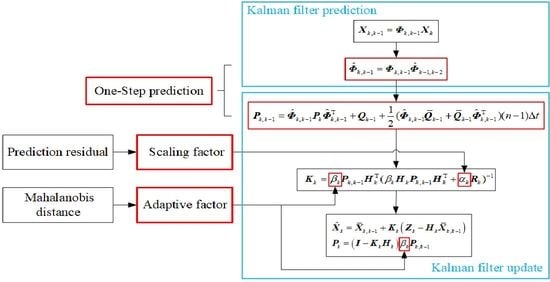
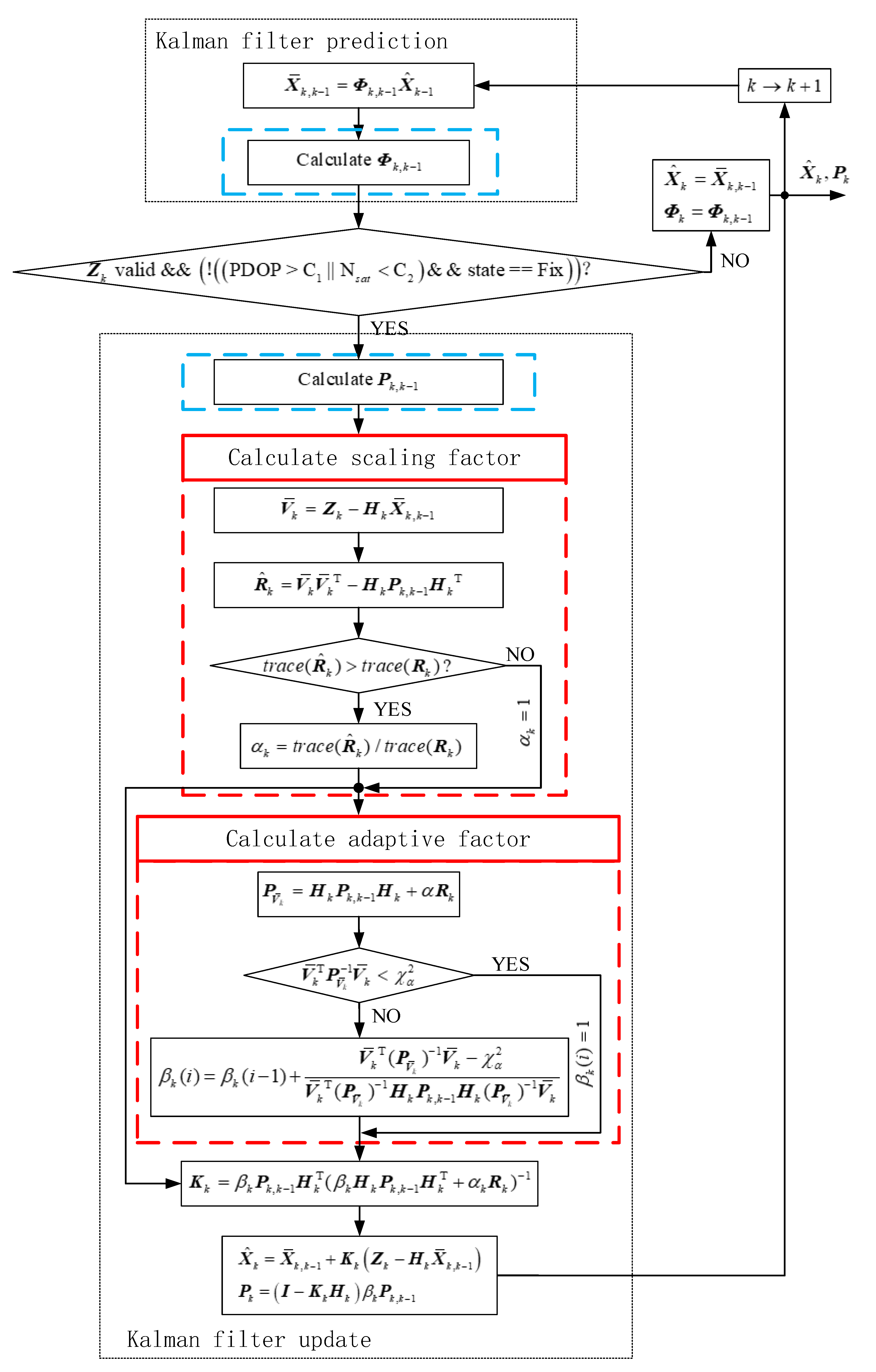
3.2.3. One-Step Prediction Kalman Filter Model

In traditional integrated navigation Kalman filter, the state prediction vector covariance matrix $P$ and state prediction vector $X$ are performed together, significantly increasing the computation load and unsuitable for systems with real-time and low power consumption requirements [5,6,34,35]. In our research, the Kalman filter is improved, and the state prediction vector covariance matrix $P$ is performed together with the measurement update, which dramatically reduces the computation load. The improved algorithm is as follows:

Prediction:

$$X_{k,k-1}={\Phi }_{k,k-1}{X}_k,$$

(32)

$${\widehat{\Phi }}_{k,k-1}={\Phi }_{k,k-1}{\widehat{\Phi }}_{k-1,k-2}$$

(33)

Update:

$$P_{k,k-1}={\widehat{\Phi }}_{k,k-1}{P}_k{\widehat{\Phi }}_{k,k-1}^{\mathrm{T}}+Q_{k-1}+\frac{1}{2}({\widehat{\Phi }}_{k,k-1}{\overline{Q}}_{k-1}+{\overline{Q}}_{k-1}{\widehat{\Phi }}_{k,k-1}^{\mathrm{T}})(n-1)\Delta t,$$

(34)

$$K_k=P_{k,k-1}{H}_k^{\mathrm{T}}{(H_k{P}_{k,k-1}{H}_k^{\mathrm{T}}+R_k)}^{-1},$$

(35)

$$X_k=X_{k,k-1}+K_k(Z_k-H_k{X}_{k,k-1}),$$

(36)

$$P_k=(I-K_k{H}_k)P_{k,k-1},$$

(37)

where $\Phi$ represents the state transition matrix; $\widehat{\Phi }$ denotes the calculated state transition matrix, which is obtained by multiplying the current $\Phi$ by the previous $\widehat{\Phi }$. For example, ${\Phi }_{k,k-1}$ means the state transition matrix from epoch $k-1$ to epoch $k$.

In order to put the state predicted covariance matrix $P$ into the measurement update process, it is necessary to use the state transition matrix $\Phi$ to achieve this goal. Therefore, theoretical reasoning is needed to prove the feasibility of the formula.

According to the theoretical derivation, $Q$ and $P$ of the $k+3$ epoch in the extended Kalman filter are as follows [36]:

$$Q_{k+2}=\frac{1}{2}({\Phi }_{k+3,k+2}{\overline{Q}}_{k+2}+{\overline{Q}}_{k+2}{\Phi }_{k+3,k+2}^{\mathrm{T}})\Delta t$$

(38)

$$\begin{array}{ll}{P}_{k+3,k+2}& ={\Phi }_{k+3,k+2}{P}_{k+2}{\Phi }_{k+3,k+2}^{\mathrm{T}}+Q_{k+2}\\ & =({\Phi }_{k+3,k+2}{\Phi }_{k+2,k+1}{\Phi }_{k+1,k})P_k{({\Phi }_{k+3,k+2}{\Phi }_{k+2,k+1}{\Phi }_{k+1,k})}^{\mathrm{T}}+Q_{k+2}+\\ & {\Phi }_{k+3,k+2}{Q}_{k+1}{\Phi }_{k+3,k+2}^{\mathrm{T}}+({\Phi }_{k+3,k+2}{\Phi }_{k+2,k+1})Q_k{({\Phi }_{k+3,k+2}{\Phi }_{k+2,k+1})}^{\mathrm{T}}\end{array},$$

(39)

where $Q$ is the constant spectral density matrix; $\Delta t$ is the sampling interval of the navigation system.

Expand the Formula (39):

$$\begin{array}{ll}{P}_{k+3,k+2}& ={\Phi }_{k+3,k+2}{P}_{k+2}{\Phi }_{k+3,k+2}^{\mathrm{T}}+Q_{k+2}\\ & =({\Phi }_{k+3,k+2}{\Phi }_{k+2,k+1}{\Phi }_{k+1,k})P_k{({\Phi }_{k+3,k+2}{\Phi }_{k+2,k+1}{\Phi }_{k+1,k})}^{\mathrm{T}}+Q_{k+2}+\\ & \frac{1}{2}[({\Phi }_{k+3,k+2}{\Phi }_{k+2,k+1}){\overline{Q}}_{k+1}{\Phi }_{k+3,k+2}^{\mathrm{T}}+{\Phi }_{k+3,k+2}{\overline{Q}}_{k+1}{({\Phi }_{k+3,k+2}{\Phi }_{k+2,k+1})}^{\mathrm{T}}]\Delta t+\\ & \frac{1}{2}[({\Phi }_{k+3,k+2}{\Phi }_{k+2,k+1}{\Phi }_{k+1,k}){\overline{Q}}_k{({\Phi }_{k+3,k+2}{\Phi }_{k+2,k+1})}^{\mathrm{T}}+({\Phi }_{k+3,k+2}{\Phi }_{k+2,k+1}){\overline{Q}}_k{({\Phi }_{k+3,k+2}{\Phi }_{k+2,k+1}{\Phi }_{k+1,k})}^{\mathrm{T}}]\Delta t\end{array},$$

(40)

where ${\overline{Q}}_k\approx {\overline{Q}}_{k+1}\approx {\overline{Q}}_{k+2}\approx \cdots \approx {\overline{Q}}_{k+n}$ is the system noise covariance matrix.

By observing Equation (40), it can be found that the first and second terms on the right side of the equation are easier to calculate, while the third and fourth terms are relatively complicated. If we want to calculate the third and fourth terms, we must save the previous value of $\Phi$. However, as time grows, the number of $\Phi$ that also needs to be saved increases, which seriously wastes hardware memory resources. Therefore, in order to facilitate the calculation, we should construct the third and fourth terms into the form of the first term, as shown below:

$$s_3=\frac{1}{2}[({\Phi }_{k+3,k+2}{\Phi }_{k+2,k+1}{\Phi }_{k+1,k}){\overline{Q}}_{k+1}+{\overline{Q}}_{k+1}{({\Phi }_{k+3,k+2}{\Phi }_{k+2,k+1}{\Phi }_{k+1,k})}^{\mathrm{T}}]\Delta t$$

(41)

$$s_4=\frac{1}{2}[({\Phi }_{k+3,k+2}{\Phi }_{k+2,k+1}{\Phi }_{k+1,k}){\overline{Q}}_k+{\overline{Q}}_k{({\Phi }_{k+3,k+2}{\Phi }_{k+2,k+1}{\Phi }_{k+1,k})}^{\mathrm{T}}]\Delta t.$$

(42)

Consequently, substituting (41) and (42) for the last two items in (40),

$$\begin{array}{ll}{P}_{k+3,k+2}=& {\Phi }_{k+3,k+2}{P}_{k+2}{\Phi }_{k+3,k+2}^{\mathrm{T}}+Q_{k+2}\\ & =({\Phi }_{k+3,k+2}{\Phi }_{k+2,k+1}{\Phi }_{k+1,k})P_k{({\Phi }_{k+3,k+2}{\Phi }_{k+2,k+1}{\Phi }_{k+1,k})}^{\mathrm{T}}+Q_{k+2}+\\ & \frac{1}{2}[({\Phi }_{k+3,k+2}{\Phi }_{k+2,k+1}{\Phi }_{k+1,k}){\overline{Q}}_{k+1}+{\overline{Q}}_{k+1}{({\Phi }_{k+3,k+2}{\Phi }_{k+2,k+1}{\Phi }_{k+1,k})}^{\mathrm{T}}]\Delta t+\\ & \frac{1}{2}[({\Phi }_{k+3,k+2}{\Phi }_{k+2,k+1}{\Phi }_{k+1,k}){\overline{Q}}_k+{\overline{Q}}_k{({\Phi }_{k+3,k+2}{\Phi }_{k+2,k+1}{\Phi }_{k+1,k})}^{\mathrm{T}}]\Delta t\end{array}.$$

(43)

In order to verify the feasibility of replacing the last two items of Formula (40) with the constructed Formulas (41) and (42), we use Formula (43) to subtract Formula (40). If the result approaches zero, it indicates that the construction method is feasible. The procedures (43)–(40) are as follows:

$$\begin{array}{ll}(43)-(40)=& \frac{1}{2}[({\Phi }_{k+3,k+2}{\Phi }_{k+2,k+1}{\Phi }_{k+1,k}){\overline{Q}}_{k+1}+{\overline{Q}}_{k+1}{({\Phi }_{k+3,k+2}{\Phi }_{k+2,k+1}{\Phi }_{k+1,k})}^{\mathrm{T}}]\Delta t-\\ & \frac{1}{2}[({\Phi }_{k+3,k+2}{\Phi }_{k+2,k+1}){\overline{Q}}_{k+1}{\Phi }_{k+3,k+2}^{\mathrm{T}}+{\Phi }_{k+3,k+2}{\overline{Q}}_{k+1}{({\Phi }_{k+3,k+2}{\Phi }_{k+2,k+1})}^{\mathrm{T}}]\Delta t+\\ & \frac{1}{2}[({\Phi }_{k+3,k+2}{\Phi }_{k+2,k+1}{\Phi }_{k+1,k}){\overline{Q}}_k+{\overline{Q}}_k{({\Phi }_{k+3,k+2}{\Phi }_{k+2,k+1}{\Phi }_{k+1,k})}^{\mathrm{T}}]\Delta t-\\ & \frac{1}{2}[({\Phi }_{k+3,k+2}{\Phi }_{k+2,k+1}{\Phi }_{k+1,k}){\overline{Q}}_k{({\Phi }_{k+3,k+2}{\Phi }_{k+2,k+1})}^{\mathrm{T}}+({\Phi }_{k+3,k+2}{\Phi }_{k+2,k+1}){\overline{Q}}_k{({\Phi }_{k+3,k+2}{\Phi }_{k+2,k+1}{\Phi }_{k+1,k})}^{\mathrm{T}}]\Delta t\end{array}.$$

(44)

According to the theoretical formula of the Kalman filter state transition matrix, it can be known that there is $\Delta t$ in the matrix, so it is assumed that ${\Phi }_k\approx I+F_k\Delta t$. In the Kalman filter, $\Delta t$ is equal to 0.01s. Putting it into Equation (44), it can be seen that (43)–(40) are high-order small quantities, and the result approaches zero. The details are as follows:

$$\begin{array}{ll}(43)-(40)=& \frac{1}{2}(\Delta t^2+F_2\Delta t^3+F_3\Delta t^3+F_2{F}_3\Delta t^4)(F_1-F_3^{\mathrm{T}}){\overline{Q}}_k+\frac{1}{2}{\overline{Q}}_k(F_1^{\mathrm{T}}-F_3)(\Delta t^2+F_2\Delta t^3+F_3\Delta t^3+F_2{F}_3\Delta t^4)-\\ & \frac{1}{2}(\Delta t^2+F_1\Delta t^3+F_2\Delta t^3+F_3\Delta t^3+F_2{F}_1\Delta t^4+F_3{F}_1\Delta t^4+F_3{F}_2\Delta t^4+F_3{F}_2{F}_1\Delta t^5){\overline{Q}}_k{(F_2+F_3+F_3{F}_2\Delta t)}^{\mathrm{T}}-\\ & \frac{1}{2}(F_2+F_3+F_3{F}_2\Delta t){\overline{Q}}_k{(\Delta t^2+F_1\Delta t^3+F_2\Delta t^3+F_3\Delta t^3+F_2{F}_1\Delta t^4+F_3{F}_1\Delta t^4+F_3{F}_2\Delta t^4+F_3{F}_2{F}_1\Delta t^5)}^{\mathrm{T}}\end{array}.$$

(45)

Therefore, the third and fourth terms of Formula (40) can be replaced by (41) and (42). The $P$ matrix of the epoch $k+3$ can be rewritten as follows:

$$\begin{array}{ll}{P}_{k+3,k}& =({\Phi }_{k+3,k+2}{\Phi }_{k+2,k+1}{\Phi }_{k+1,k})P_k{({\Phi }_{k+3,k+2}{\Phi }_{k+2,k+1}{\Phi }_{k+1,k})}^{\mathrm{T}}+Q_{k+2}+\\ & 2\cdot \frac{1}{2}[({\Phi }_{k+3,k+2}{\Phi }_{k+2,k+1}{\Phi }_{k+1,k}){\overline{Q}}_k+{\overline{Q}}_k{({\Phi }_{k+3,k+2}{\Phi }_{k+2,k+1}{\Phi }_{k+1,k})}^{\mathrm{T}}]\Delta t\end{array},$$

(46)

where $P_{k+3,k}$ is the state predicted covariance matrix from epoch $k$ to epoch $k+3$. It can be seen from the above formula that the calculation of the state prediction covariance matrix from epoch $k$ to $k+3$ can be realized in one step. Then, the state transition matrix from epoch $k$ to epoch $k+3$ can be written as:

$${\Phi }_{k+3,k}={\Phi }_{k+3,k+2}{\Phi }_{k+2,k+1}{\Phi }_{k+1,k}.$$

(47)

Similarly, the matrix of $P$ and $\Phi$ are extended to $n$ epochs, namely from $k$ epochs to $k+n$ epochs, as follows:

$$\begin{array}{ll}{P}_{k+n,k}& ={\Phi }_{k+n,k}{P}_k{\Phi }_{k+n,k}^{\mathrm{T}}+\frac{1}{2}({\Phi }_{k+n,k+n-1}{\overline{Q}}_{k+n-1}+{\overline{Q}}_{k+n-1}{\Phi }_{k+n,k+n-1}^{\mathrm{T}})\Delta t\\ & +\frac{1}{2}({\Phi }_{k+n,k}{\overline{Q}}_{k+n-1}+{\overline{Q}}_{k+n-1}{\Phi }_{k+n,k}^{\mathrm{T}})(n-1)\Delta t\end{array}$$

(48)

$${\Phi }_{k+n,k}={\Phi }_{k+n,k+n-1}{\Phi }_{k+n-1,k+n-2}\cdots {\Phi }_{k+2,k+1}{\Phi }_{k+1,k}$$

(49)

Therefore, the $P$ can be executed in the measurement update process, and in the Kalman filter prediction process, a new $\Phi$ can be obtained by multiplying each previous $\Phi$. The state transition matrix $\Phi$ and the predicted state vector covariance matrix $P$ of the code running in the chip can be written in the following form:

$${\widehat{\Phi }}_{k,k-1}={\Phi }_{k,k-1}{\widehat{\Phi }}_{k-1,k-2}$$

(50)

$$P_{k,k-1}={\widehat{\Phi }}_{k,k-1}{P}_k{\widehat{\Phi }}_{k,k-1}^{\mathrm{T}}+Q_{k-1}+\frac{1}{2}({\widehat{\Phi }}_{k,k-1}{\overline{Q}}_{k-1}+{\overline{Q}}_{k-1}{\widehat{\Phi }}_{k,k-1}^{\mathrm{T}})(n-1)\Delta t.$$

(51)

In Kalman filter prediction, the amount of calculation of the $\Phi$ matrix is much less than that of $P$ matrix, which significantly reduces the computational complexity.

4. Experimental Route and Hardware Platform

This study selected a section of complex scene road in Wuhan, Hubei Province as the test route, as shown in Figure 2. The route includes scenes such as Boulevard 1, Tunnel 1, Boulevard 2, and Tunnel 2. They constitute a continuous GNSS high occlusion scene, and there are continuous s-turns and up and down ramps, and multipath interference of lake reflected signals. The vehicle-mounted experimental platform is shown in Figure 3. The testing equipment and reference equipment are installed on the vehicle’s roof, and the odometer is attached to the wheel. The experimental equipment is a multi-sensor fusion navigation and positioning module, which incorporates single-frequency GNSS, MEMS-IMU, magnetometer, barometer, temperature and humidity sensor, NB-IoT, and e-sim to form an integrated navigation and positioning system. The reference equipment is NovAtel SPAN CPT6, a navigation-level device with dual-frequency GNSS and fiber optic gyroscope tight integrated navigation technology.

Table 1. Performance specifications of the IMU in the experiment.

		Module	SPAN CPT6
Gyro	Bias (deg/h)	10	0.027
	ARW (deg/sqrt(h))	0.27	0.0667
Accelerometer	Bias (mGal)	1800	50
	VRW (m/s/sqrt(h))	0.042	0.03

shows the performance indicators of the two devices.

5. Results

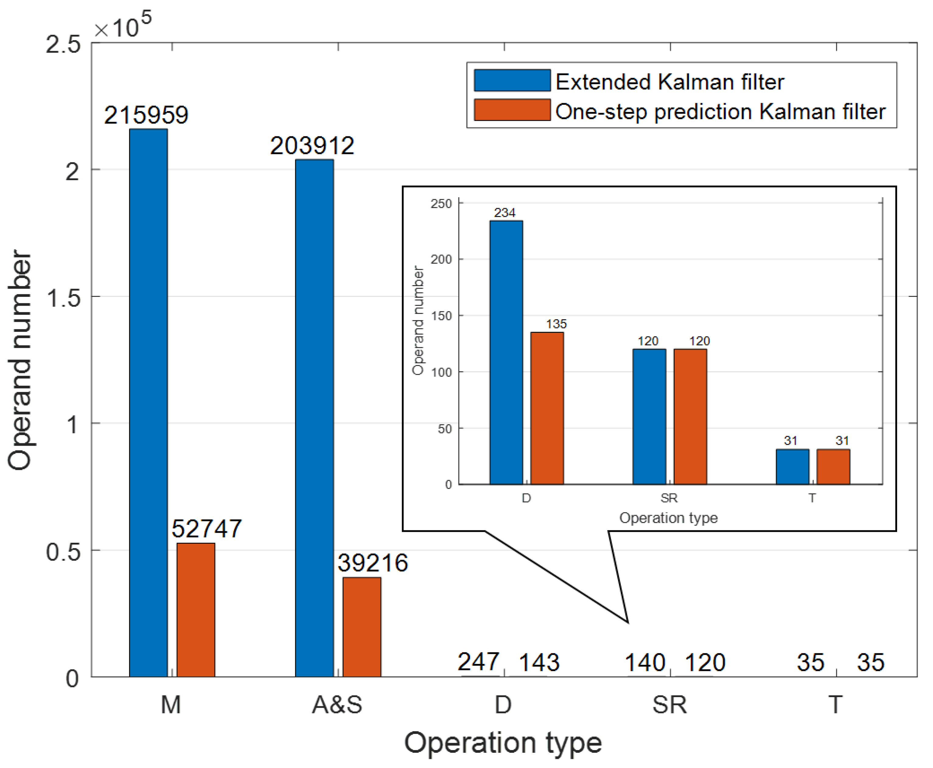
5.1. Operands Analysis and Comparison

In order to verify the effectiveness of the simplified one-step prediction Kalman filter in the improved robust adaptive algorithm, the calculation amount and positioning performance are analyzed and compared with the extended Kalman filter.

In the IRAKF algorithm, the simplified one-step prediction Kalman filter is used. That is, the prediction state covariance matrix is only calculated once in the measurement update cycle. Consequently, the algorithm dramatically reduces calculation and can run in real-time in a low-cost MCU with a low operating frequency. It ensures that the system works with low power consumption. In order to evaluate the computational complexity of the one-step prediction Kalman filter and extended Kalman filter in the IRAKF algorithm, the operation number of multiplication (M), addition and subtraction (A&S), division (D), square root (SR), and trigonometric (T) function are counted. Figure 4 shows the number of each operation in the two Kalman filters. In the extended Kalman filter, the operands of M, A&S, D, SR, and T within one second are 215,959, 203,912, 247, 132, and 35, respectively. In the one-step prediction Kalman filter, the operands of M, A&S, D, SR, and T are 52,747, 39,216, 143, 132, and 35, respectively. Compared with the extended Kalman filter algorithm, the one-step prediction Kalman filter reduces the number of operations of M by 75.6%, A&S by 80.8%, and D by 42.1%.

In order to verify whether the simplified one-step prediction Kalman filter in the IRAKF algorithm will affect the positioning performance of the integrated navigation system, the real-time vehicle-mounted experiments are carried out in a challenging urban environment. Meanwhile, the simplified one-step prediction Kalman filter is replaced with the extended Kalman filter in the algorithms, and the positioning accuracy of the two is compared. The positioning errors of the two in the North, East, and Down directions are shown in Figure 5. It can be seen from the figure that although the simplified one-step prediction Kalman filter reduces the number of operations of the algorithm, its positioning accuracy hardly deteriorates. The overlap curve in Figure 5a is expanded to the separation curve in Figure 5b to make the figures clearer.

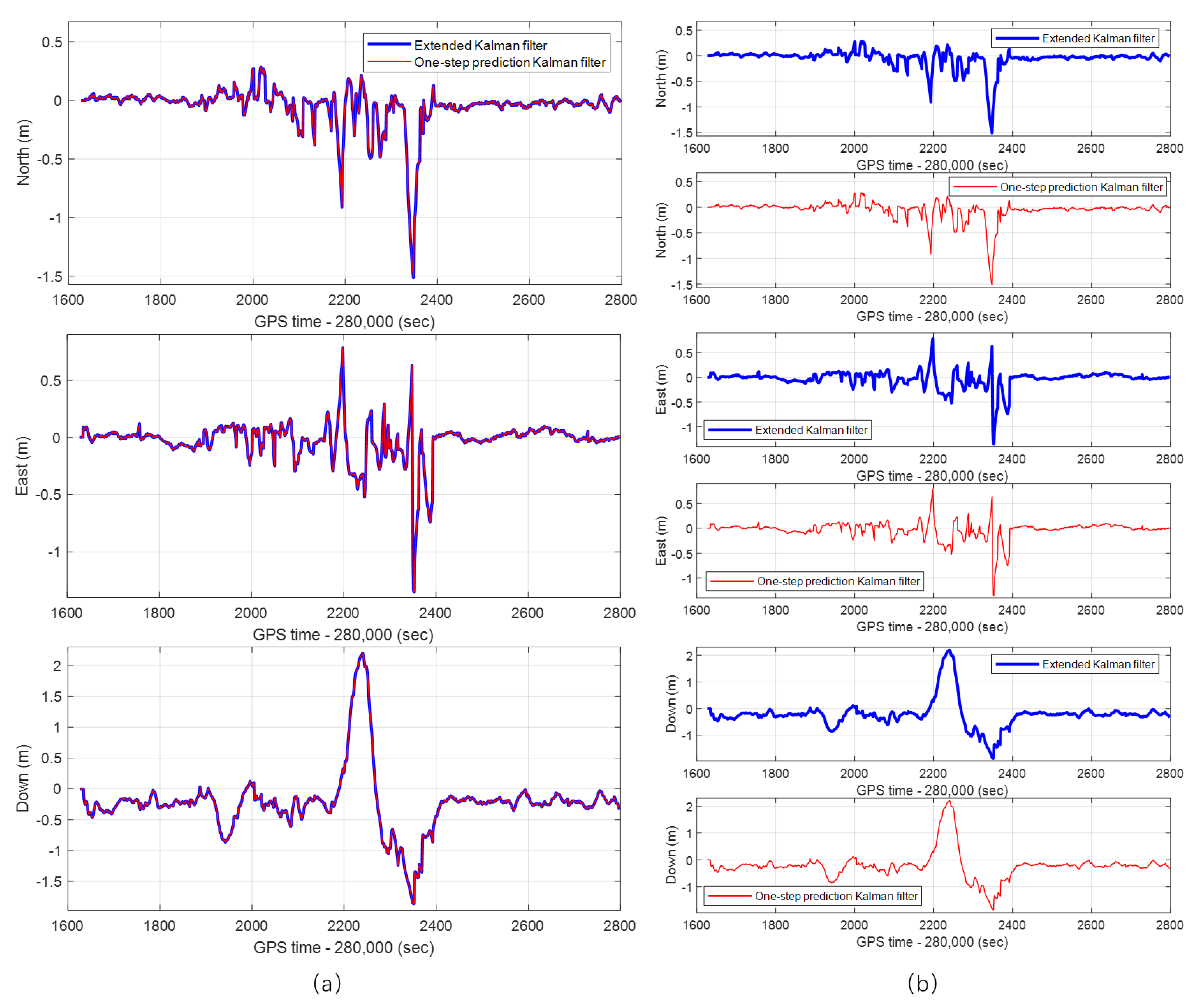
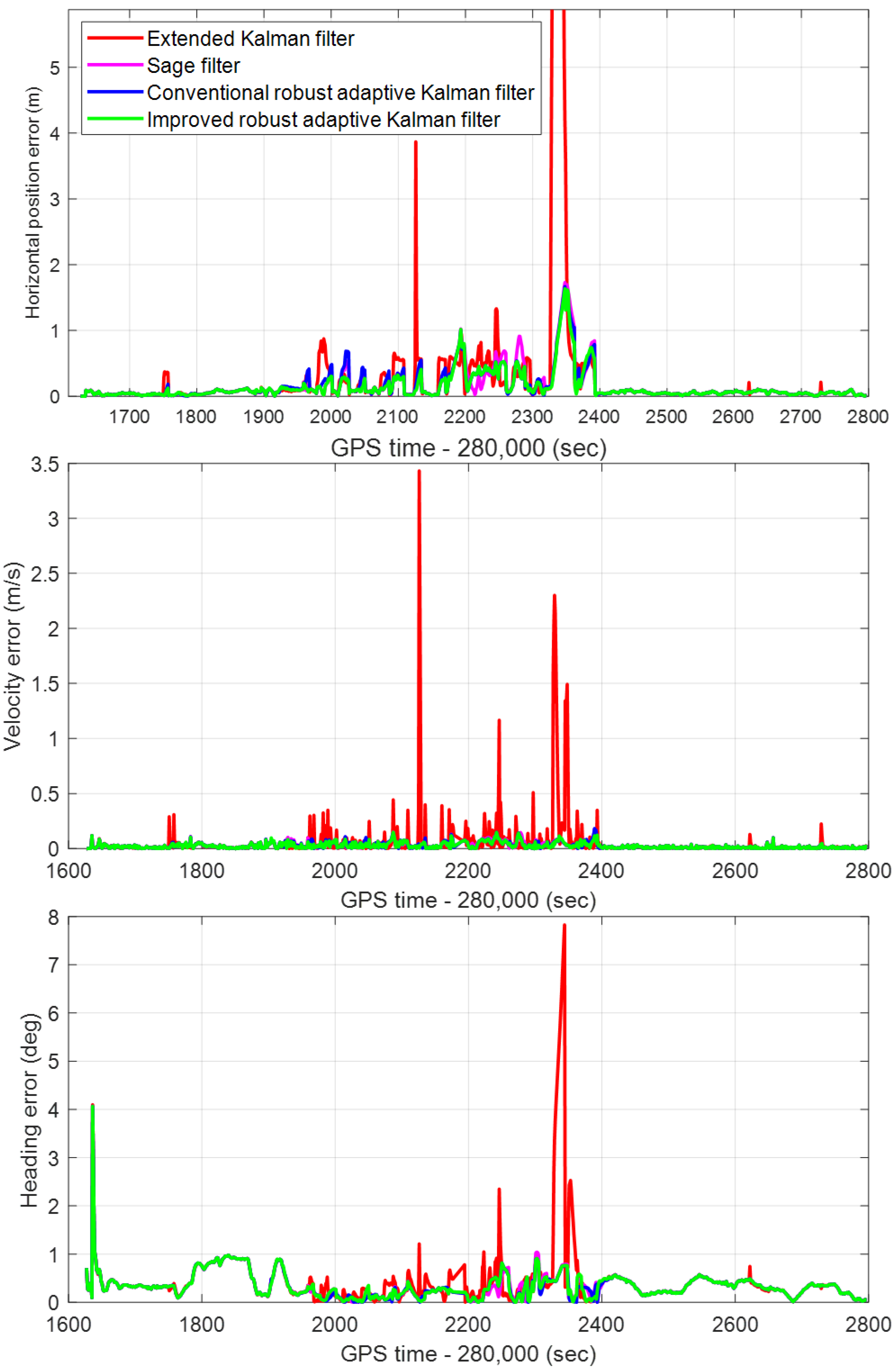
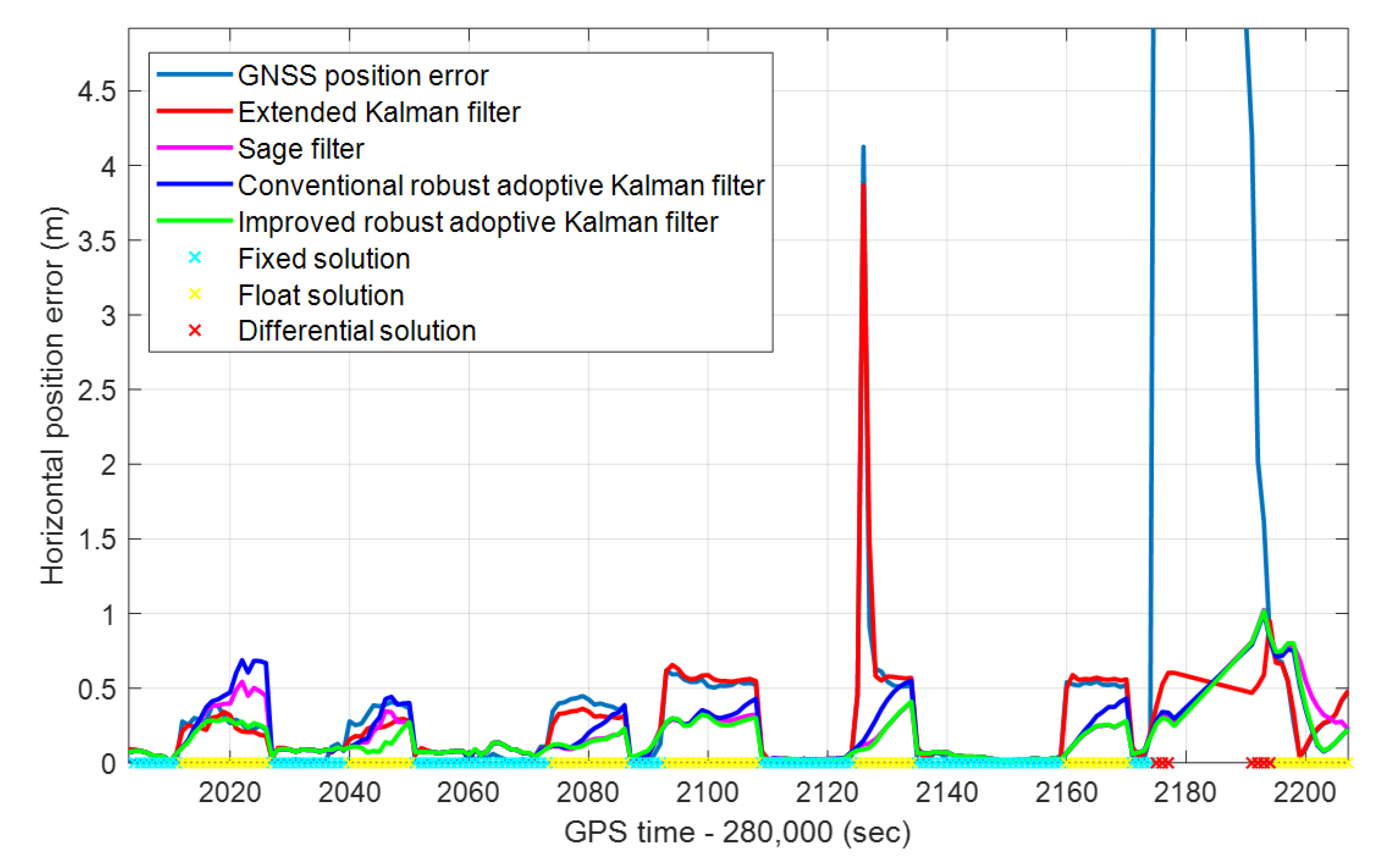
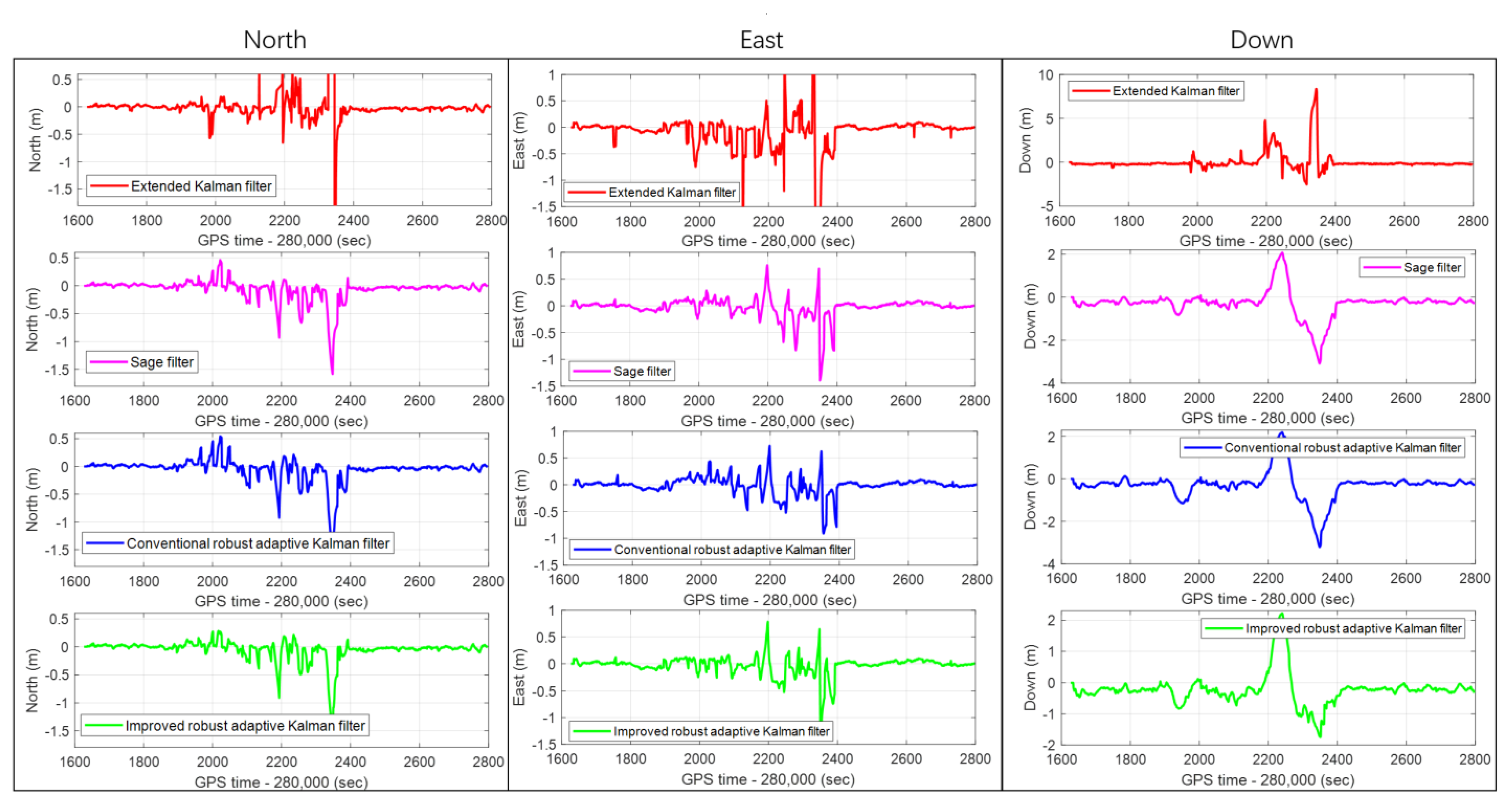
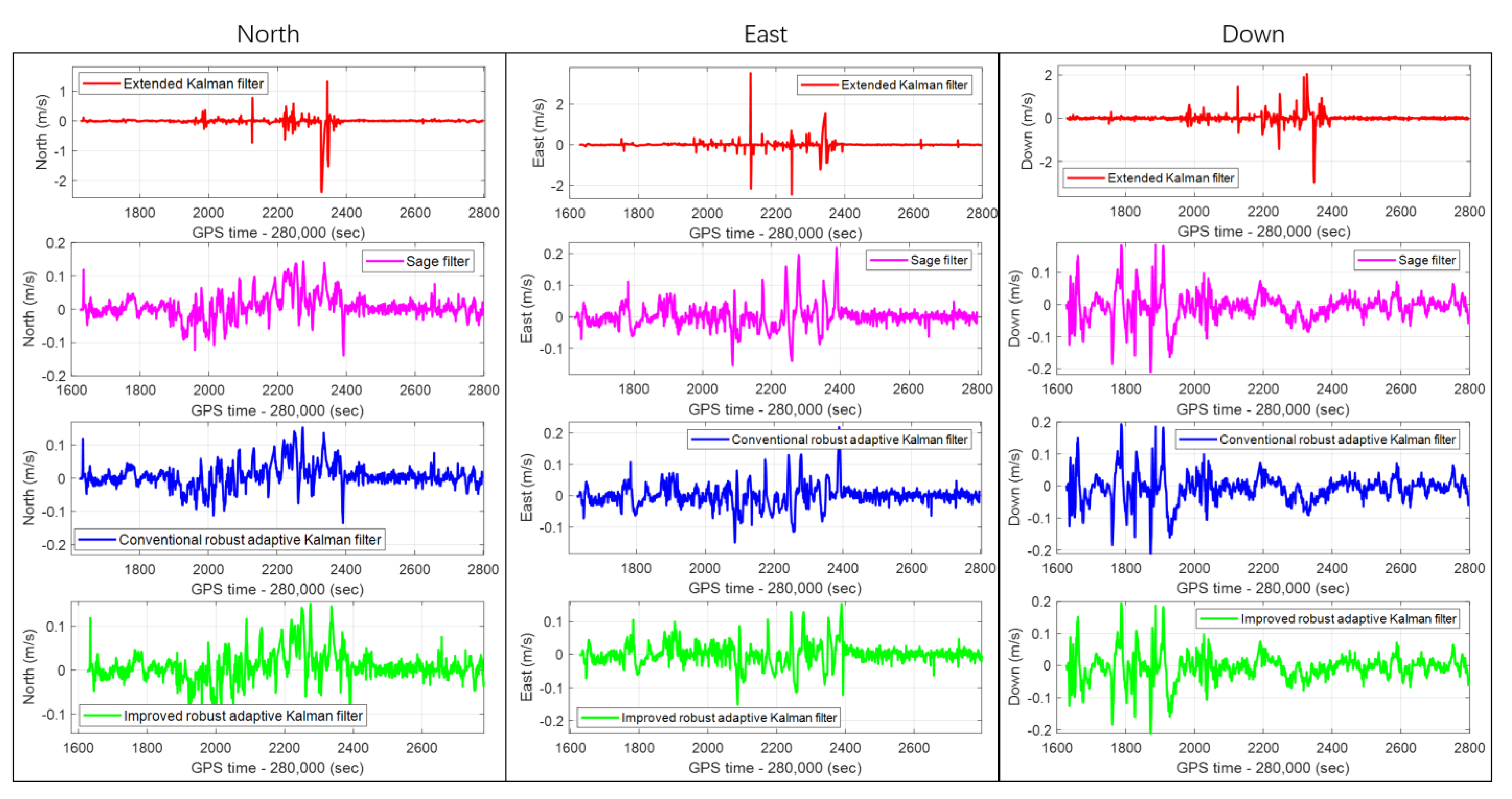
5.2. Performance Verification

The accuracy of the positioning, velocity, and attitude are essential indicators that reflect the performance of the integrated navigation system. In order to verify the performance of the IRAKF algorithm in complex scenarios, real-time vehicle-mounted experiments are carried out. This section analyzes the horizontal positioning, forward velocity, and heading errors of the single-frequency GNSS/MEMS-IMU/odometer integrated navigation module with the IRAKF algorithm. In addition, the positioning performance of challenging scenes, namely boulevard and tunnel, is also analyzed and compared.

The horizontal position, forward velocity, and heading errors of the whole test route estimated by the methods of the CRAKF, Sage filter, extended Kalman filter, and IRAKF are shown in Figure 6. It can be noted that the horizontal position error of the extended Kalman filter exhibits large values between 281,989 s (280,000 + 1989) and 282,344 s (280,000 + 2344). Compared with the CRAKF, Sage filter, extended Kalman filter, the IRAKF algorithm proposed in this paper has the highest positioning accuracy and the best robustness. But it is only limited to most road scenes. The main reason is that the GNSS receiver cannot output the observation vector covariance matrix, and the manually set value cannot accurately represent the current positioning error. In terms of horizontal velocity error, it can be seen from Figure 6 that the proposed IRAKF can provide better performance than the other three methods. From the heading error in Figure 6, it can be seen that the heading error of IRAKF is smaller than the other three methods in most periods and the error curve is smoother. To make the figures clearer, the subfigures of horizontal position error, velocity error, and heading error are shown in Figure 7, showing the curves in each figure.

The statistical values of the root mean square (RMS) and maximum errors of the horizontal position, forward velocity, and heading of the CRAKF, Sage filter, extended Kalman filter, and IRAKF are shown in

Table 2. The RMS and maximum errors of the horizontal position, forward velocity, and heading of the CRAKF, Sage filter, extended Kalman filter, and IRAKF.

	CRAKF			Sage Filter			Extended Kalman Filter			IRAKF
	Pos (m)	Vel (m/s)	Heading (deg)	Pos (m)	Vel (m/s)	Heading (deg)	Pos (m)	Vel (m/s)	Heading (deg)	Pos (m)	Vel (m/s)	Heading (deg)
RMS	0.26	0.038	0.44	0.28	0.039	0.46	1.3	0.22	0.77	0.25	0.035	0.43
MAX	1.67	0.18	4.06	1.7	0.18	4.1	17.1	3.4	7.8	1.65	0.14	4.06

. It can be seen that the RMS and maximum errors of the proposed IRAKF are minor than those of the other three methods. The specific comparative analysis is as follows. Compared with the CRAKF, the RMS errors of the horizontal position, forward speed, and heading of the IRAKF are increased by 3.8%, 7.9% and 2.3%, respectively. Compared with Sage filtering, it has increased by 10.7%, 10.3% and 6.5% respectively. However, compared with extended Kalman filter, it has increased by 80.7%, 84.1%, and 44.2%, respectively. In terms of maximum error, the horizontal position, forward speed and heading of IRAKF are improved by 1.2%, 22.2% and 0%, respectively compared with the CRAKF. Compared with Sage filtering, it is improved by 2.9%, 22.2% and 1% respectively. However, compared with extended Kalman filter, it has increased by 90.4%, 95.9% and 47.9%, respectively.

The single-frequency GNSS signal is easy to block on the boulevard, resulting in poor positioning accuracy. As shown in Figure 8, the GNSS signal was blocked at the epoch of 282,126 s, and there was an abnormal observation. At this time, the GNSS positioning error reached 4.12 m. The single-frequency GNSS/MEMS-IMU/odometer integrated navigation positioning error with extended Kalman filter algorithm is also 3.8 m. Although the CRAKF can suppress abnormal GNSS positioning errors, it is still inferior in reducing error divergence. It can be seen from the green line in Figure 8 that the proposed IARKF has the best accuracy, preventing abnormal GNSS observations and effectively slowing down the divergence of positioning errors.

In the boulevard scene, the horizontal position errors of the CRAKF, Sage filter, extended Kalman filter, and IRAKF at the moment of GNSS abnormal observations are shown in

Table 3. The horizontal position error of CRAKF, Sage filter, extended Kalman filter, and IRAKF at the moment of gross error.

	CRAKF	Sage Filter	Extended KF	IRAKF	Improvement (%)
horizontal position (m)	0.15	0.14	3.8	0.12	20	14.3	96.8

. It can be seen that the integrated navigation system with the IRAKF eliminates GNSS gross errors and improves positioning accuracy. Compared with the other three methods, its positioning accuracy at the time of GNSS gross errors are improved by 20%, 14.3%, and 96.8%, respectively.

The tunnel scene significantly influences the positioning accuracy, and if it is not processed, a significant error will occur. The GNSS signal is blocked when the vehicle enters the tunnel, and only the odometer assists the INS. However, the GNSS RTK is a pseudo-fixed solution when the vehicle enters the tunnel, as shown at 282,327 s in Figure 9. If sufficient measures are not taken, the GNSS pseudo-fixed solution with large errors will disturb the stable integrated navigation system, leading to significant errors in subsequent positioning results. The red line in the figure shows the impact of the integrated navigation with the extended Kalman filter algorithm. At the time of the GNSS outliers, the fixed solution positioning error reaches 2.1 m. Nevertheless, the positioning error with the IRAKF is only 0.14 m. This value is also better than the 0.165 m and 0.16 m of Sage filter and CRAKF. Besides, the divergence speed of the INS in the tunnel is slower than the other three methods. Therefore, the IRAKF eliminates the RTK pseudo-fixed solution, improves the stability of the system state and reduces the positioning error.

In the tunnel scene, the horizontal position errors of the CRAKF, Sage filter, extended Kalman filter, and IRAKF at the moment of GNSS RTK pseudo-fixed solution are shown in

Table 4. The horizontal position errors of the CRAKF, Sage filter, extended Kalman filter, and IRAKF at the moment of GNSS RTK pseudo-fixed solution in the tunnel scene.

	CRAKF	Sage Filter	Extended KF	IRAKF	Improvement (%)
horizontal position (m)	0.16	0.165	2.1	0.14	12.5	15.2	93.3

. It can be seen from the table that the integrated navigation system with IRAKF eliminates GNSS abnormal observation and improves positioning accuracy. Compared with the other three methods, its positioning accuracy at the RTK pseudo-fixed solution epoch is improved by 12.5%, 15.2%, and 93.3%, respectively.

5.3. Comparison with Other Filtering Algorithms

The IRAKF algorithm is verified in the single-frequency GNSS/MEMS-IMU/odometer integrated navigation module, and compared with the CRAKF, Sage filter, and extended Kalman filter. The real-time errors of the position, velocity and attitude of the four algorithms in the entire experimental route are shown in Figure 10, Figure 11 and Figure 12, respectively. In addition, to make the graph clearer, the subfigures of the position, velocity, and attitude errors are shown in Figure 13, Figure 14 and Figure 15, respectively, which show each curve in the figure. It can be seen from the figures that, in complex scenes such as Boulevard 1, Tunnel 1, Boulevard 2, and Tunnel 2, the position, velocity, and attitude errors are relatively large. In these scenarios, the integrated navigation system with the extended Kalman filter algorithm is difficult to reduce the positioning error caused by the GNSS gross error. Although the integrated navigation with the Sage filter and CRAKF algorithms can achieve a certain effect, the performance is still unsatisfactory in some harsh environments. However, the proposed IRAKF can effectively eliminate GNSS gross errors, slow down system divergence errors in complex environments, and improve the position, velocity and attitude accuracy of single-frequency GNSS/MEMS-IMU/odometer integrated navigation.

In the entire experimental route, the RMS errors of the position, velocity, and attitude of the CRAKF, Sage filter, extended Kalman filter, and IRAKF are shown in

Table 5. The RMS errors of the position, velocity, and attitude of the CRAKF, Sage filter, extended Kalman filter, and IRAKF in the whole experimental route.

	Position (m)			Velocity (m/s)			Attitude (deg)
	North	East	Down	North	East	Down	Roll	Pitch	Yaw
CRAKF	0.21	0.16	0.74	0.035	0.034	0.045	0.53	0.214	0.432
Sage filter	0.2	0.19	0.68	0.036	0.036	0.044	0.55	0.22	0.45
Extended Kalman filter	1.11	0.66	1.02	0.19	0.2	0.23	0.65	0.60	0.774
IRAKF	0.18	0.14	0.56	0.033	0.032	0.043	0.51	0.2	0.43

. Since the extended Kalman filter has weak robustness, its RMS errors of the position, velocity and attitude are relatively large. The CRAKF, Sage filter, and IRAKF can eliminate gross errors, and their performance indexes are better than the extended Kalman filter. However, according to the data in Table 5, the proposed IRAKF has the best performance. In terms of positioning accuracy, compared with the CRAKF algorithm, IRAKF has improved by 14.3%, 12.5%, and 24.3% in the north, east, and down directions, respectively. Compared with the Sage filter, it has improved by 10%, 26.3%, and 17.6%, respectively. However, compared with the extended Kalman filter, it is improved by 83.7%, 78.7%, and 45.1%, respectively.

5.4. Real-Time Power Consumption Verification and Comparision

In the process of real-time vehicle navigation, the power meter and power supply are used to test the power consumption of the multi-sensor fusion navigation and positioning module, and the data are saved. The real-time power consumption curve is shown in Figure 16. The MCU operating frequency in the module with the IRAKF algorithm can be reduced to 50 MHz, and its average power consumption is 143 mW. Because CRAKF, Sage filter, and extended Kalman filter do not adopt Kalman one-step prediction strategy, the working frequency of MCU can only be reduced to 200 MHz. The average power consumption of these methods is relatively high—296 mW, 300 mW, and 304 mW, respectively. According to the above analysis, IRAKF reduces the module’s power consumption by reducing the computational complexity.

6. Discussion

In this paper, robustness and low computation complexity are the topics. According to the presented results, the IRAKF applied to single-frequency GNSS/MEMS-IMU/odometer integrated navigation in the challenging urban environment can improve the robustness ability of the system and significantly reduce the computational complexity of the algorithm. Compared with the CRAKF, Sage filter, and extended Kalman filter algorithms, the IRAKF with the one-step prediction Kalman filter dramatically reduces computation. As shown in Figure 4, the number of M, A&S, and D operations decreased by 75.6%, 80.8%, and 42.3%, respectively. The IRAKF not only reduces the amount of calculation but also slows down the error divergence. As shown in Figure 6, the maximum errors of horizontal position, forward speed, and the heading of CRAKF are 1.67 m, 0.18 m/s, and 4.06 degrees, respectively. For the Sage filter they are 1.7 m, 0.18 m/s, and 4.1 degrees, respectively, and for the extended Kalman filter they are 17.1 m, 3.4 m/s, and 7.8 degrees, respectively. However, for the IRAKF they are only 1.65 m, 0.14 m/s, and 4.06 degrees, respectively. Regarding the RMS errors, the horizontal position, forward speed, and heading of the IRAKF are 0.29 m, 0.04m/s, and 0.72 degrees, respectively.

Compared with the CRAKF, Sage filter, and extended Kalman filter algorithm, the IRAKF improves robustness. In the boulevard, when the GNSS signal is blocked suddenly, the positioning result becomes worse. Since the covariance matrix of the observation vector is a fixed value, the gain matrix of the extended Kalman filter cannot change with the GNSS positioning accuracy, so the influence of these outliers cannot be eliminated. However, the IRAKF algorithm can use the scale and adaptive factors to adjust the measurement vector and state prediction covariance matrices. The gain matrix can change with the GNSS positioning accuracy and improve the robust performance of the integrated navigation system. As shown in Figure 8, the IRAKF suppresses the abnormal GNSS and improves the positioning accuracy of integrated navigation. In addition, it also has a specific effect in terms of improving the accuracy of the tunnel scene. When the vehicle enters the tunnel, GNSS RTK is a pseudo-fixed solution. The IRAKF can eliminate the RTK pseudo-fixed solution and reduce the system state error. However, sometimes the positioning error of the IRAKF is greater than the CRAKF, Sage filter, and extended Kalman filter. The main reason is that the observation vector covariance matrix is an artificially set fixed value, which cannot accurately represent the current GNSS positioning accuracy. If the GNSS receiver can output the observation vector covariance matrix, it is believed that the positioning accuracy of the integrated navigation system with the IARKF will be further improved.

In addition, since the calculation amount of the IRAKF algorithm is less than that of the CRAKF, Sage filter, and extended Kalman filter, the MCU with the IRAKF algorithm can run at a lower operating frequency. As can be seen from Figure 16, compared with the other three algorithms, IRAKF has the lowest power consumption.

7. Conclusions

This paper presents an improved robust adaptive Kalman filter algorithm with real-time performance and low computation complexity for single-frequency GNSS/MEMS-IMU/odometer integrated navigation in the challenging environment. It is implemented in multi-sensor fusion navigation and positioning module. The algorithm obtains the scale factor by the prediction residual to adjust the artificially set covariance matrix of the observation vector under different GNSS solution states. It can make the observation vector covariance matrix constantly change with complex scenes. Since the Mahalanobis distance can better reflect the disturbance anomaly, the Mahalanobis distance based on the prediction residual is introduced to detect disturbance anomalies and obtain the adaptive factor to inflate the state prediction covariance matrix. Furthermore, the one-step prediction Kalman filter is adopted to reduce the computation complexity of the algorithm and realize the low power consumption real-time integrated navigation.

The robust adaptive algorithm based on the GNSS state suppresses the GNSS gross errors in the avenue scene, eliminates the GNSS-RTK pseudo-fixed solution in the tunnel scene, and improves the positioning accuracy of integrated navigation. In addition, compared with the CRAKF, Sage filter, and extended Kalman filter, the IRAKF reduces the amount of calculation and realizes the low power consumption of the integrated navigation module. The average power consumption in the whole test route is only 143 mW. It is of great significance for real-time vehicle navigation applications in complex environments. With measurements from the multi-sensor fusion navigation and positioning module, the proposed filtering method can provide real-time medium and low dynamic horizontal positioning error of less than 0.25 m, a forward velocity error of less than 0.035m/s, and a heading error of less than 0.43 degrees, which are far better than the results of the same level commercial integrated navigation module or other existing filtering methods.

References

1. Grewal, M.; Andrews, A.; Bartone, C. Global Navigation Satellite Systems, Inertial Navigation, and Integration; John Wiley & Sons: Hoboken, NJ, USA, 2020. [Google Scholar] [CrossRef]
2. Kaplan, E.D.; Hegarty, C. Understanding GPS Principles and Applications; Artech House Publishers: Boston, MA, USA, 2005. [Google Scholar]
3. Gallon, E.; Joerger, M.; Pervan, B. Development of Stochastic IMU Error Models for INS/GNSS Integration. In Proceedings of Proceedings of the 34th International Technical Meeting of the Satellite Division of The Institute of Navigation (ION GNSS+ 2021), St. Louis, MI, USA, 20–24 September 2021; pp. 2565–2577. [Google Scholar]
4. Shin, E.H. Estimation Techniques for Low-Cost Inertial Navigation. Ph.D. Thesis, The University of Calgary, Calgary, AB, Canada, 2005. [Google Scholar]
5. Hu, S.; Xu, S.; Wang, D.; Zhang, A. Optimization Algorithm for Kalman Filter Exploiting the Numerical Characteristics of SINS/GPS Integrated Navigation Systems. Sensors 2015, 15, 28402–28420. [Google Scholar] [CrossRef]
6. Niu, X.; Zhang, Q.; Gong, L.; Liu, C.; Zhang, H.; Shi, C.; Wang, J.; Coleman, M. Development and evaluation of GNSS/INS data processing software for position and orientation systems. Surv. Rev. 2015, 47, 87–98. [Google Scholar] [CrossRef]
7. Chang, G. Robust Kalman filtering based on Mahalanobis distance as outlier judging criterion. J. Geod. 2014, 88, 391–401. [Google Scholar] [CrossRef]
8. Zhao, L.; Qiu, H.; Feng, Y. Analysis of a robust Kalman filter in loosely coupled GPS/INS navigation system. Measurement 2016, 80, 138–147. [Google Scholar] [CrossRef]
9. Jiang, C.; Zhang, S.B.; Zhang, Q.Z. A New Adaptive H-Infinity Filtering Algorithm for the GPS/INS Integrated Navigation. Sensors 2016, 16, 2127. [Google Scholar] [CrossRef] [Green Version]
10. Teunissen, P.J.G. Quality control in integrated navigation systems. In Proceedings of the IEEE Symposium on Position Location and Navigation. A Decade of Excellence in the Navigation Sciences, Las Vegas, NV, USA, 20–23 March 1990; pp. 158–165. [Google Scholar]
11. Jiang, C.; Zhang, S.-b.; Zhang, Q.-z. A Novel Robust Interval Kalman Filter Algorithm for GPS/INS Integrated Navigation. J. Sens. 2016, 2016, 1–7. [Google Scholar] [CrossRef] [Green Version]
12. Jiang, C.; Zhang, S.B. A Novel Adaptively-Robust Strategy Based on the Mahalanobis Distance for GPS/INS Integrated Navigation Systems. Sensors 2018, 18, 695. [Google Scholar] [CrossRef] [Green Version]
13. Gao, B.; Hu, G.; Zhu, X.; Zhong, Y. A Robust Cubature Kalman Filter with Abnormal Observations Identification Using the Mahalanobis Distance Criterion for Vehicular INS/GNSS Integration. Sensors 2019, 19, 5149. [Google Scholar] [CrossRef] [Green Version]
14. Yang, Z.; Li, Z.; Liu, Z.; Wang, C.; Sun, Y.; Shao, K. Improved robust and adaptive filter based on non-holonomic constraints for RTK/INS integrated navigation. Meas. Sci. Technol. 2021, 32, 105110. [Google Scholar] [CrossRef]
15. Yang, Y.; Xu, T. An Adaptive Kalman Filter Based on Sage Windowing Weights and Variance Components. J. Navig. 2003, 56, 231–240. [Google Scholar] [CrossRef]
16. Mohamed, A.H.; Schwarz, K.P. Adaptive Kalman Filtering for INS/GPS. J. Geod. 1999, 73, 193–203. [Google Scholar] [CrossRef]
17. Wang, J.; Stewart, M.P.; Tsakiri, M. Adaptive Kalman Filtering for Integration of GPS with GLONASS and INS; Springer: Berlin/Heidelberg, Germany, 2000; Volume 121, pp. 325–330. [Google Scholar]
18. Gandhi, M.A.; Mili, L. Robust Kalman Filter Based on a Generalized Maximum-Likelihood-Type Estimator. IEEE Trans. Signal Process. 2010, 58, 2509–2520. [Google Scholar] [CrossRef]
19. Duan, Z.; Zhang, J.; Zhang, C.; Mosca, E. Robust H2 and H∞ filtering for uncertain linear systems. Automatica 2006, 42, 1919–1926. [Google Scholar] [CrossRef]
20. Zhang, L.; Viktorovich, P.A.; Selezneva, M.S.; Neusypin, K.A. Adaptive Estimation Algorithm for Correcting Low-Cost MEMS-SINS Errors of Unmanned Vehicles under the Conditions of Abnormal Measurements. Sensors 2021, 21, 623. [Google Scholar] [CrossRef]
21. Zhao, L.; Liu, J. An Improved Adaptive Filtering Algorithm with Applications in Integrated Navigation. In Proceedings of the 2012 Third International Conference on Digital Manufacturing & Automation, Guilin, China, 31 July–2 August 2012; pp. 182–185. [Google Scholar]
22. Shi, E. An Improved Real-Time Adaptive Kalman Filter for Low-Cost Integrated GPS/INS Navigation. In Proceedings of the 2012 International Conference on Measurement, Information and Control, Harbin, China, 18–20 May 2012; Volume 2, pp. 1093–1098. [Google Scholar]
23. Yang, Y.; He, H.B.; Xu, G. Adaptively robust filtering for kinematic geodetic positioning. J. Geod. 2001, 75, 109–116. [Google Scholar] [CrossRef]
24. Yang, Y.; Cui, X. Adaptively robust filter with multi adaptive factors. Surv. Rev. 2013, 40, 260–270. [Google Scholar] [CrossRef]
25. Yang, Y. Adaptively Robust Kalman Filters with Applications in Navigation. In Sciences of Geodesy-I; Springer: Berlin/Heidelberg, Germany, 2010; pp. 49–82. [Google Scholar]
26. Yang, Y.; Xu, T.; Xu, J. Principles and Comparisons of Various Adaptively Robust Filters with Applications in Geodetic Positioning. In Proceedings of the 1st International Workshop on the Quality of Geodetic Observation and Monitoring Systems (QuGOMS’11), Munich, Germany, 13–15 April 2011; pp. 101–105. [Google Scholar]
27. Jung, S.; Hwang, S.; Shin, H.; Shim, D.H. Perception, Guidance, and Navigation for Indoor Autonomous Drone Racing Using Deep Learning. IEEE Robot. Autom. Lett. 2018, 3, 2539–2544. [Google Scholar] [CrossRef]
28. Rostami, M.; Kolouri, S.; Eaton, E.; Kim, K. SAR Image Classification Using Few-Shot Cross-Domain Transfer Learning. In Proceedings of the 2019 IEEE/CVF Conference on Computer Vision and Pattern Recognition Workshops (CVPRW), Long Beach, CA, USA, 16–17 June 2019; pp. 907–915. [Google Scholar]
29. Abdallah, A.; Kassas, Z. Deep Learning-Aided Spatial Discrimination for Multipath Mitigation; IEEE: Piscataway, NJ, USA, 2020; pp. 1324–1335. [Google Scholar]
30. Fayjie, A.; Hossain, S.; Doukhi, O.; Lee, D. Driverless Car: Autonomous Driving Using Deep Reinforcement Learning in Urban Environment. In Proceedings of the 2018 15th International Conference on Ubiquitous Robots (UR), Jeju, Korea, 28 June–1 July 2018; pp. 896–901. [Google Scholar]
31. Yan, P.; Jiang, J.; Tang, Y.; Zhang, F.; Xie, D.; Wu, J.; Liu, J.; Liu, J. Dynamic Adaptive Low Power Adjustment Scheme for Single-Frequency GNSS/MEMS-IMU/Odometer Integrated Navigation in the Complex Urban Environment. Remote. Sens. 2021, 13, 3236. [Google Scholar] [CrossRef]
32. Zhou, Y.; Chen, Q.; Niu, X. Kinematic Measurement of the Railway Track Centerline Position by GNSS/INS/Odometer Integration. IEEE Access 2019, 7, 157241–157253. [Google Scholar] [CrossRef]
33. Simon, D. Optimal State Estimation (Kalman, H∞, and Nonlinear Approaches)||Optimal Smoothing; John Wiley and Sons: Hoboken, NJ, USA, 2006; pp. 263–296. [Google Scholar]
34. Zhu, Q.J.; Yan, G.M.; Yang, P.X.; Qin, Y.Y. A Rapid Computation Method for Kalman Filtering in Vehicular SINS/GPS Integrated System. Appl. Mech. Mater. 2012, 182–183, 541–545. [Google Scholar] [CrossRef]
35. Emami, M.; Taban, M. A Low Complexity Integrated Navigation System for Underwater Vehicles. J. Navig. 2018, 71, 1–17. [Google Scholar] [CrossRef]
36. Li, Q.; Ban, Y.; Niu, X.; Zhang, Q.; Gong, L.; Liu, J. Efficiency Improvement of Kalman Filter for GNSS/INS through One-Step Prediction of P Matrix. Math. Probl. Eng. 2015, 2015, 1–13. [Google Scholar] [CrossRef]
Figure 1. The algorithm flow chart of improved robust adaptive Kalman filter algorithm applied to GNSS/INS/odometer integrated navigation module.
Remotesensing 13 04317 g001
Figure 2. Real-time performance verification experiment trajectory and scenes of vehicle navigation.
Remotesensing 13 04317 g002
Figure 3. Vehicle experimental platform.
Remotesensing 13 04317 g003
Figure 4. The operand number of the operation type in the extended Kalman filter and the one-step prediction Kalman filter.
Remotesensing 13 04317 g004
Figure 5. The positioning errors of the extended Kalman filter and the one-step prediction Kalman filter in North, East, and Down directions: (a) curve overlap; (b) curve separation.
Remotesensing 13 04317 g005
Figure 6. The real-time horizontal position error, velocity error, and heading error of the conventional robust adaptive Kalman filter, Sage filter, extended Kalman filter, and improved robust adaptive Kalman filter.
Remotesensing 13 04317 g006
Figure 7. The real-time horizontal position error, velocity error, and heading error subfigures of conventional robust adaptive Kalman filter, Sage filter, extended Kalman filter, and improved robust adaptive Kalman filter.
Remotesensing 13 04317 g007
Figure 8. The positioning errors of conventional robust adaptive Kalman filter, Sage filter, extended Kalman filter, improved robust adaptive Kalman filter, and GNSS in the boulevard scene.
Remotesensing 13 04317 g008
Figure 9. The positioning errors of conventional robust adaptive Kalman filter, Sage filter, extended Kalman filter, improved robust adaptive Kalman filter, and GNSS in the tunnel scene.
Remotesensing 13 04317 g009
Figure 10. The real-time position errors of the CRAKF, Sage filter, extended Kalman filter, and IRAKF in the North, East, and Down directions in the whole experimental route.
Remotesensing 13 04317 g010
Figure 11. The real-time velocity errors of the CRAKF, Sage filter, extended Kalman filter, and IRAKF in the North, East, and Down directions in the whole experimental route.
Remotesensing 13 04317 g011
Figure 12. The real-time attitude errors of the CRAKF, Sage filter, extended Kalman filter, and IRAKF in the Roll, Pitch, and Yaw in the whole experimental route.
Remotesensing 13 04317 g012
Figure 13. The real-time position errors subfigures of the CRAKF, Sage filter, extended Kalman filter, and IRAKF in the North, East, and Down directions.
Remotesensing 13 04317 g013
Figure 14. The real-time velocity errors subfigures of the CRAKF, Sage filter, extended Kalman filter, and IRAKF in the North, East, and Down directions.
Remotesensing 13 04317 g014
Figure 15. The real-time attitude errors subfigures of the CRAKF, Sage filter, extended Kalman filter, and IRAKF in the Roll, Pitch, and Yaw.
Remotesensing 13 04317 g015
Figure 16. The real-time power consumption of IRAKF, CRAKF, extended Kalman filter, and Sage filter in the experimental route.
Remotesensing 13 04317 g016