Abstract
Turbidity impacts the growth and productivity of marine benthic habitats due to light limitation. Daily/monthly synoptic and tidal influences often drive turbidity fluctuations, however, our understanding of what drives turbidity across seasonal/interannual timescales is often limited, thus impeding our ability to forecast climate change impacts to ecologically significant habitats. Here, we analysed long term (18-year) MODIS-aqua data to derive turbidity and the associated meteorological and oceanographic (metocean) processes in an arid tropical embayment (Exmouth Gulf in Western Australia) within the eastern Indian Ocean. We found turbidity was associated with El Niño Southern Oscillation (ENSO) cycles as well as Indian Ocean Dipole (IOD) events. Winds from the adjacent terrestrial region were also associated with turbidity and an upward trend in turbidity was evident in the body of the gulf over the 18 years. Our results identify hydrological processes that could be affected by global climate cycles undergoing change and reveal opportunities for managers to reduce impacts to ecologically important ecosystems.
1. Introduction
Coastal ecosystems make contributions to marine productivity and biodiversity yet are increasingly the most threatened of all oceanic regions [1,2,3,4]. Habitats such as coral reefs, seagrasses and intertidal zones are under local pressure from changes in water quality that arise from a range of naturally occurring (e.g., cyclones) and anthropogenic processes (e.g., dredging). On global scales, climate change is increasingly altering a range of meteorological and oceanographic (metocean) processes that have likewise contributed to the decline of coastal ecosystems. The impacts of climate change include ocean warming and acidification [5,6], coastal wind intensification [7], the increasing frequency and severity of extreme weather events [8], changing wave climates [9], and sea level rise [10] which are often strongly coupled to global climate cycles such as El Niño–Southern Oscillation (ENSO) and the Indian Ocean Dipole (IOD) [11,12,13]. While these pressures from climate change often have long-lasting impacts, any co-occurring local declines in water quality, such as increasing water turbidity, can also reduce the recovery and resilience of many ecologically critical habitats [14].
Turbidity is one of the most important measures of water quality from an ecological perspective, given its close association with light that fuels the primary productivity of coastal ecosystems [15]. For example, corals and seagrasses are important benthic habitats that rely on light for photosynthesis. Low light availability due to increased suspended matter not only stunts growth but can smother benthic habitats, transport toxins, and reduce larval recruitment [16] and species diversity [16,17,18,19]. There is also some evidence that turbidity can become a stressor that increases corals’ susceptibility to bleaching [20]. However, some moderate levels of disturbance, such as turbidity fluctuations, can also be associated with increased levels of biodiversity in the context of the intermediate disturbance hypothesis [21], and some turbid water corals show a higher resilience to bleaching than their clear water counterparts [22,23,24].
Understanding how turbidity impacts coastal habitats is complicated by the fact that natural turbidity regimes can be highly variable in space and time [25,26]. Therefore, to assess if turbidity is causing ecological stress or if turbidity is likely changing with environmental drivers over time, it is necessary to understand the long-term (multi-decadal) turbidity regime and its spatial variability across a region, and to determine the associated metocean drivers of that regime. While regional processes such as tides, wind and waves are often found to be major drivers of turbidity [27,28], global climate cycles can influence these regional processes and therefore have implications for regional variability on inter-annual timescales. For example, large scale wind and wave patterns are modified by ENSO/IOD and have impacts on regional oceanographic processes [29]. To better predict the effects of climate variability and change on coastal ecosystems, an understanding of how both regional and large-scale metocean processes are driving turbidity patterns is required.
Identifying the drivers of regional-scale turbidity variability requires combining long term, high spatial and temporal resolution turbidity observations with corresponding metocean data. Traditional field methods for turbidity data collection (e.g., placement of turbidity loggers) cannot meet the spatial and temporal requirements that are necessary for this type of analysis as they represent a single location and may not capture the full range of synoptic and climate influences within a region. Satellite derived remote sensing, however, overcomes these limitations by providing both long-term (multi-decadal) time series, and broad (100′s km2) spatial scale datasets [30,31].
Remotely sensed turbidity data is based on reflectance values of a water body, that increase in the presence of suspended matter. While the accuracy has been validated by a large body of work globally [32], there are some limitations to consider when utilising remote sensing in coastal waters. Foremost among these is the performance of ocean colour algorithms, that must be calibrated for each regional body of water due to distinct differences in optical properties between regions [33]. A further limitation is the presence of cloud cover, which, if present at the time of satellite overpass, results in no data for that pass. This is problematic when time series analysis against variable synoptic influences (e.g., wind) is required, particularly for satellites with a low temporal frequency, such as the National Aeronautics and Space Administration (NASA) Landsat platform, with a 16-day revisit cycle [34]. A better alternative is NASA’s Moderate Resolution Imaging Spectroradiometer (MODIS) satellite, which has the advantage of a daily revisit cycle and has been in orbit continually since 1999 (MODIS-terra)/2002 (MODIS-aqua), meaning multi-decadal time series studies, with high temporal resolution, are now feasible.
To better understand the long-term variability of turbidity and implications for vulnerable ecosystems, a more detailed understanding of the drivers of turbidity fluctuations is needed. In this work we quantified 18 years of daily turbidity in the Exmouth Gulf, derived from the MODIS-aqua satellite [35], to provide a unique dataset that we use to investigate long-term trends in turbidity. Firstly, we investigate the spatial and temporal variability of turbidity across the environmentally heterogenous Gulf region and determine patterns related to seasonal and inter-annual variability. We then focus on the potential metocean drivers of turbidity, and the influence of ENSO and IOD. This novel analysis is important for understanding how drivers of turbidity vary across low to high energy gradients, as well as for predicting how climate change could affect turbidity and therefore marine ecosystems. This information will also provide important insights for managers of the region’s unique environmental values.
2. Materials and Methods
2.1. Study Site
The Exmouth Gulf is a large embayment (~3000 km2) with a maximum depth of 20 m (LAT), situated in the arid tropical Pilbara region of Western Australia (Figure 1). The Gulf supports one of Australia’s most fauna rich coastal regions and has previously been nominated for World Heritage status [36,37,38]. Yet, anthropogenic impacts including prawn trawling [39] and offshore oil and gas [40,41] are present threats in the region. Further, several large-scale industrial developments have been proposed for Exmouth Gulf in recent times leading to calls by government for a very high level of protection to be given to the eastern and southern portion of the Gulf [42].
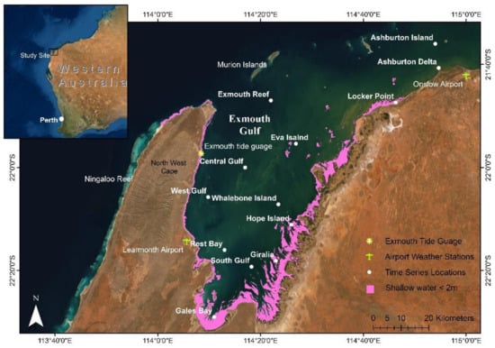
Figure 1.
The study site, Exmouth Gulf, located in northern Western Australia. Symbols represent 13 locations where long-term turbidity and its metocean drivers are analysed, location of the Exmouth tide gauge and location of the airport weather stations. Pink areas denote shallow water where satellite derived bathymetry estimates depths of less than two metres during lowest astronomical tides. Note: Some sites are named for their proximity to known landmarks and may not represent the exact location of that landmark. Basemap images are from Environmental Systems Research Institute (ESRI) Online.
Lying to the east of Cape Range, the Gulf marks the transition zone from the deep ocean waters adjacent to the fringing Ningaloo Reef to the shallow, broad (up to 250 km) North West Shelf. The World Heritage protected Ningaloo Reef’s northern extent lies within the north-west corner of the Gulf and ocean currents and tides may provide some connectivity between their ecosystems [43]. The complex topography of islands, reefs and shoals produce a variety of wave patterns that, combined with a heterogenous sediment size distribution, results in a natural spatial variability of sediment dynamics and turbidity [44].
The northern Gulf is influenced by wind-driven waves to 1.5 m, with a seasonally variable wave climate where longer period energy (peak period ~7–10 s) ocean swell waves propagate into the Gulf during austral winter from the NNW and shorter period, locally generated sea waves (peak period ~5 s) during the austral summer from the SSW [45]. Regional wind patterns are due to low pressure troughs extending over the inland Pilbara during summer resulting in a mostly south to south-easterly regime. However, localised sea breezes are often present due to differential land/sea temperatures causing predominantly south-westerly and north-easterly wind patterns year-round [36].
The eastern gulf shoreline consists of tidal creeks with extensive, low relief salt flats (>1000 km2) which are lined with highly productive intertidal microbial mats (~80 km2) and mangroves (161 km2) [46]. The north-eastern coast is subject to wave energy that is fetch limited by the dimensions of the Gulf, while the south-eastern coast is tidal current dominated [36]. On a daily timescale, currents on the North West Shelf tend to be dominated by tides [47]. While tides are thought to be a major force behind sediment transport in the Exmouth Gulf, the extent to which they influence turbidity is not known. Tides are semi-diurnal and force the Gulfs circulation in a north–south orientation, with average spring tides to 2.5 m and a mean tidal range of 1.5 m (AHD).
There are no permanent river systems that drain into the Gulf and rainfall is low (~300 mm annually), typically occurring between January and July in association with tropical lows/cyclones. Cyclones form 1–3 times a year on average, mostly during La Niña phases [48], with a severe cyclone (Category 5) directly impacting the Gulf approximately every 25 years. In the past these cyclones have caused some irreversible impacts to reefs, seagrasses, mangroves and foredunes, significantly altered nearshore bathymetry and water flow paths, and shifted entire tidal creeks [36,49].
The Exmouth Gulf was chosen for this study as it is a region where there is both high spatial and temporal variability in turbidity as well as ecologically critical marine habitats and proximity to a World Heritage listed marine park (Ningaloo Reef). There are industrial pressures in the region and the Environmental Protection Agency has advised that all Exmouth Gulf proposals will be subject to a cumulative impact study [42]. From a global perspective, the region is subject to influences from both the Pacific Ocean and Indian Ocean climatic events which makes an interesting case study for the effects and interactions of large-scale climatic drivers such as El-Niño Southern Oscillation and the Indian Ocean Dipole.
2.2. Remote Sensing Data
The satellite-derived remote sensing data used here were MODIS-Aqua level 1B scenes from 2002–2020 that were downloaded from the NASA LAADS DAAC (https://ladsweb.modaps.eosdis.nasa.gov (accessed on 12 January 2021)). The Level 1B products were converted to atmospherically corrected, at-surface remote sensing reflectance using the Level 1 to Level 2 generator (L2gen) function on SeaDAS 7.4 (https://seadas.gsfc.nasa.gov/ (accessed on 20 January 2021)). During the L2Gen process the standard MODIS atmospheric correction model was replaced by the Management Unit of the Mathematical Model of the North Sea (MUMM) atmospheric correction process which has shown better reflectance retrieval for turbid coastal waters [50]. This resulted in 7640 Level 2 product files that were then geo-referenced using the geolocation file associated with each image (scene) and gridded to Plate Carrée projection at 250 m resolution. As cloud cover is a constraint for remote sensing analyses, a data count was conducted over the north-eastern (Ashburton Island), northern (Exmouth Reef) and southern (South Gulf) regions of the Gulf to check how seasonally variable scene availability was in the region. The highest scene availability was in August (420–450) and the lowest in January (190–250).
A single band total suspended matter (TSM) algorithm based on the red band reflectance at 667 nm was applied to all scenes. Reflectance at this wavelength is sensitive to the concentration of suspended sediments [15]. The algorithm employed here was developed by Dorji and Fearns [51] and was calibrated and validated with in situ measurements in the same optically complex waters of this study region. In moderately turbid waters the algorithm detects sediments in the top approximately 50 cm of water and is considered robust at depths greater than approximately 2 m in mildly turbid waters [51]. As some near-coastal regions of the Exmouth Gulf may be shallower than 2 m during some tidal cycles (Figure 1), some caution should be applied to the analysis of these regions.
2.3. Spatial and Temporal Variability in Turbidity
Daily, monthly, and annual mean turbidity as total suspended matter (TSM) were calculated for each pixel of the Gulf (each pixel represents a 250 × 250 m ground area). Annual anomaly maps were produced to identify years where turbidity was higher or lower than the long-term (2002–2020) mean turbidity. The anomalies were calculated annually from July 1 to June 31, both to capture Austral Summer in each map and because MODIS-aqua’s first data acquisition was in July 2002. To quantify how turbidity varied at different locations throughout the Exmouth Gulf, 13 specific locations were chosen to extract a monthly time series on which to conduct statistical analyses (Figure 1). The locations were chosen to represent sites that were (a) spatially and ecologically distinct; (b) had varying levels of wave/swell exposure; (c) where a priori mapping showed significant correlations to different environmental variables existed.
To assess for long term monotonic trends (overall increase or decline in turbidity) at each location, a modified Mann–Kendall test for serially correlated data using the Hamed and Rao [52] variance correction approach (95% confidence interval) was applied to all monthly time series. This test removes the autocorrelation effect of time series data increasing the reliability of the statistical result. To assess how seasonality might affect turbidity, Kruskal–Wallis tests were conducted at all locations to look for significant differences between turbidity during the different months of the year at the different locations. Statistics were performed using R Studio [53]. Daily TSM time series data at each location were assessed for periodicity using spectral analysis. A derivative of Fourier transform, the Lomb–Scargle Periodogram, was used due to its superior performance where uneven sampling periods exist [54,55]. Lomb–Scargle periodograms were constructed for all locations where a turbidity time series had been extracted to assess patterns of turbidity.
2.4. Metocean Drivers of Turbidity
This analysis was separated into two parts to include both the individual time series locations (single pixel per location) and entire geographic regions (every pixel of each scene) and covered the time period January 2003–October 2019. The time period of this analysis was slightly shorter than the spatial and temporal variability of turbidity analysis (July 2002–December 2020) due to the availability of some environmental data (wave data). The following environmental variables were considered in this analysis: u and v components of the wind, wave power, tidal maxima, tidal range, mean sea level, rainfall, ENSO and IOD. There are other variables that may influence turbidity in coastal regions such as currents and internal waves, however, the data availability for these parameters is extremely limited and resource intensive (if even possible) to derive and were therefore were not considered in this analysis.
2.4.1. Individual Locations in the Gulf
To quantify the contribution of metocean processes to turbidity in the Exmouth Gulf, stepwise regression models were constructed for each of the 13 time series locations. Environmental variables that showed a significant Pearson’s r correlation with turbidity were included in the initial step of the regression, with the least significant variables removed at each step. An Akaike information criterion (AIC) test was used to find the best of the stepped models, being the one that explains the greatest amount of variation using the fewest possible independent variables (lowest AIC). The AIC compares models to find the model with the best ‘fit’ and is known to minimise the risk of choosing a bad model [56]. Monthly average values were used for all variable inputs including ENSO and IOD indexes, wave power, east–west and north–south components of the wind, rainfall and mean sea level (each variable described in Section 3.3.1); monthly mean was also used for turbidity (TSM). A separate Pearson’s correlation analysis was performed against turbidity and the three-day tidal range average to ensure this variable was captured at finer timescales. Note that environmental variables were considered at the same value for all locations in the Gulf, except for waves, which were extracted independently for each time series location.
2.4.2. Regional Analysis of Turbidity Drivers in the Gulf Using Every Pixel of the Map (Each Turbidity Data Point)
Maps representing the Pearson’s r correlations between monthly turbidity and different environmental variables (ENSO and IOD indexes, wave power, east–west and north–south components of the wind, rainfall, tidal range, tidal maxima and mean sea level), at every pixel of the region were produced. Maps showing significant p-values of these Pearson’s r correlations were also produced.
To visualise the relationship between metocean drivers and turbidity, a principal components analysis was conducted and applied for each turbidity signal (pixel) of the Gulf. The resulting maps show each pixel’s strength of association with the first three principal components (PC1, PC2 and PC3). Regions showing similar strong associations to PC1 (and to a lesser extent PC2 and PC3) were grouped together and a biplot was constructed to graphically visualise these regions and their environmental drivers.
2.4.3. Environmental Variables
Wave Power
Wave data was extracted from a 20-year regional-scale, fully coupled wave-circulation hindcast (Delft3D-SWAN [45]) that has been extensively validated along the Pilbara coast [57]. Point data was extracted for the 13 locations from 2003 to 2019. Proportional wave power (p) was calculated using the equation p = H2T, where H2 is the squared significant wave height and T is the peak wave period. For the regional analysis, the wave data grid was interpolated from the modelled spherical/nested grid to a Plate Carree cylindrical projection to match the gridded MODIS TSM data.
Wind Forcing
Strong wind conditions are known to contribute to sediment resuspension by increasing wave activity [58,59]. To investigate the effect of wind speed and direction on turbidity in the Exmouth Gulf monthly averaged wind speed and direction was calculated using Bureau of Meteorology (BOM) wind data from the regions two closest stations, at Learmonth and Onslow airports (Figure 1). Two separate wind vector components representing the magnitude and direction of East–West (u-wind) and North–South (v-wind) winds were created. A positive u is defined as being towards the east and a positive v is defined as towards the north.
Tides and Sea Surface Height
Water-level observations (relative to the Australian height datum, AHD) from 2003 to 2019 were obtained from the Exmouth tide gauge (see Figure 1) provided by the Western Australia Department of Transport (DoT). For tidal range, the difference between the maximum and minimum tidal height over each daily tidal period was calculated and the mean monthly tidal range was used in all the analyses. As this signal does not capture smaller time scale variability of tides and their effects on turbidity, we also calculated a three-day tidal range average and performed a separate correlation analysis with the turbidity value each third day through the study period (2003–2019), at each of the 13 time series locations.
Tidal maxima are thought to increase suspended sediments by both inundating depositional shorelines that are beyond the reach of normal daily tides, and by being associated with spring tidal currents. Tidal maxima were recorded as the single highest tidal height for each month (2003–2019) and used in all analyses. This signal will capture storm surges and other seasonal inundation events.
Non-tidal sources of sea level variability can potentially be a large influence in this region. Monthly mean sea level (MSL) was accessed from the Permanent Service for Mean Sea Level (PSMSL) and applied in all analyses.
Rainfall
Monthly mean rainfall was calculated from Australian Bureau of Meteorology data collected and averaged from two regional weather stations, Learmonth Airport and Onslow Airport (Figure 1). Rainfall in this region is highest from January to July, peaking in June, and the driest period is in Austral Spring.
Southern Oscillation Index (SOI) and Indian Dipole Mode (IDM)
The Southern Oscillation Index (SOI) describes the positive and negative phase of the El Niño–Southern Oscillation (ENSO), an important climate phenomenon that drives global weather patterns, and strongly affects the tropics [60]. The index is a measure of the pressure difference between opposite sides of the Pacific Ocean that leads to cyclic patterns of warming/cooling of ocean temperature and changing sea levels across the Pacific that are also transmitted into the Indian Ocean. A strongly positive SOI (>1) refers to the La Niña phase of ENSO, while a strongly negative SOI (<1) refers to the El Niño phase of ENSO. The Indian Dipole Mode (IDM) describes the positive (pIOD) and negative phase of the Indian Ocean Dipole (IOD) and is a measure of the anomalous sea surface temperature (SST) gradient between the western and eastern Indian Ocean.
The relationship between ENSO and IOD is complex. Both indices oscillate between positive and negative phases at different times and are considered related to the extent that one can trigger a shift in the other phase [61,62]. When both ENSO and IOD phases interact, they can enhance or limit both the evolution and climatic effects of both phases [62]. Correlation and regression analyses were used to measure the relationship between ENSO and turbidity, IOD and turbidity, and between ENSO and IOD. As it is known that there can be a lag time between the index phases and subsequent effects at the extremities of the oceanic regions they influence, lag correlations were calculated for 0–12-month lags, and the strongest correlating lag (10-month lag) was used in the analysis.
To analyse how the different phase combinations might affect turbidity we separated the phases into four stage types, (1): negative SOI-negative IDM; (2): negative SOI-positive IDM; (3): positive SOI-negative IDM; (4): positive SOI-positive IDM. Kruskal–Wallis analyses were applied to test for significant differences in turbidity levels between the four different phase combinations at the direct phase time and for 12 monthly lag intervals.
3. Results
3.1. Spatial and Temporal Variability in Turbidity
Turbidity varied spatially throughout the Exmouth Gulf. The highest mean TSM values (between 3.8 and 5.8 mg/L) occur at the mouth of the Ashburton Delta, along the north-east coast of the Gulf, and within Gales and Giralia Bays located at the very southern end of Exmouth Gulf. High TSM values also occur along the shallow inshore waters along the Gulf’s north-eastern and eastern coasts which are characterised by extensive mangrove and estuarine environments. Mean TSM decreased with distance offshore and increasing water depth. Lowest mean TSM values occurred in deeper water areas located in the NW part of the Gulf (Figure 2).
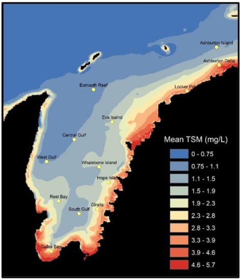
Figure 2.
Mean monthly turbidity (TSM) in the Exmouth Gulf region over the period 2002–2020, retrieved from MODIS-aqua remotely sensed data with a locally calibrated turbidity algorithm applied.
Analysis of annual turbidity anomalies spanning the 18-year time MODIS time series (July to June) shows negative TSM anomalies across much of the Gulf between 2002/03 and 2009/10 (Figure 3). This trend is reversed from 2010/11 to 2012/13 with positive TSM anomalies, particularly along the eastern Gulf. The years 2013/14 saw much of the Gulf return to negative TSM conditions with all but the very southern Gulf experiencing positive values. Between 2016/2017 and 2019/20 the Gulf experienced generally neutral TSM conditions, becoming more negative along the eastern coast.
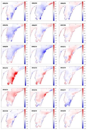
Figure 3.
Anomaly maps showing the years 2002–2020 (1 July–30 June) where mean turbidity is higher (red) or lower (blue) than the overall mean turbidity for the entire period.
3.2. Time Series Analysis of Spot Locations
Of the 13 spot locations situated around the Gulf, inshore sites exhibited the highest mean and most variable TSM values, with the site situated off the front of the Ashburton Delta returning the highest mean monthly value of 3.8 mg/L (Figure 4a). Offshore sites exhibited minimal variation with mean monthly TSM values ranging between 1 and 1.5 mg/L, but several areas saw TSM spikes of up to 3.7 mg/L. Long term trend analysis (Modified Mann–Kendall test) applied to the 13 spot locations revealed three sites located inside the Gulf (Eva Island, p < 0.01; Whalebone Island and West Gulf (p < 0.001)) had experienced a significant upward trend from 2002 to 2020, with a step increase in mean monthly TSM values occurring between 2011 and 2012. For Eva and Whalebone Island, located in the more turbid eastern Gulf, this increase was on the order 1 mg/L while the West Gulf site saw as step increase of 0.3 mg/L. TSM values did fall after 2013 but have not returned to their pre 2010 values, with TSM fluctuating between 1 and 2 mg/L at Eva and Whalebone and between 1 and 1.2 mg/L at West Gulf (Figure 4b; Mann–Kendall table of results in Appendix A). One location (Ashburton Delta) showed a small, but significant downward trend in turbidity over the study period (Table A1).
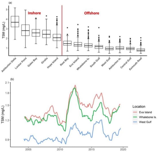
Figure 4.
(a) Monthly total suspended matter (TSM) variability at 13 locations in the Exmouth Gulf between 2002 and 2020 showing median, interquartile ranges, max/min, and outliers; offshore refers to locations more than 3 nautical miles from the coastline. (b) TSM time series (18-month rolling mean) at three locations where there was an increasing trend of monthly average TSM from 2002 to 2020 (modified Mann–Kendall p < 0.05).
All locations within Exmouth Gulf exhibited a high degree of seasonality, with mean monthly TSM differing significantly in all months (Kruskal–Wallis p < 0.01; Figure 5), and seasonal trends coinciding within similar regions of the Gulf. For example, sites located across the top of the Gulf exhibited elevated TSM during winter months and lower values during summer months, with Locker and Ashburton Delta showing the most obvious summer–winter TSM pattern with Exmouth Reef and Eva Island exhibiting the same pattern but to a lesser extent. Ashburton Island site was the anomaly showing the opposite trend higher TSM value in autumn and spring and lower values in winter and summer. This autumn–spring pattern was observed at sites located across the middle of Exmouth Gulf including Central Gulf, West Gulf, Whalebone and Hope Islands. Southern Gulf sites including Rest and Gales Bays, South Gulf and Giralia exhibit a spring peak in mean monthly TSM with only Rest Bay having an autumn peak, with the other sites exhibiting lower mean monthly TSM across the rest of the year.
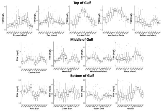
Figure 5.
Monthly differences in average turbidity (TSM mg/L) from 13 different locations in the Exmouth Gulf 2002–2020.
Spectral analysis of daily TSM supports the observed seasonal turbidity trends. For example, those sites experiencing a single winter TSM peak return a very strong spectral frequency of 360 days while sites that experience autumn and spring peaks returned a spectral analyses frequency spike at 180 days. Sites located in the southern Gulf, including Giralia, Hope Island, Gales and Rest Bay were also found to exhibit a spectral frequency spike at 14 days, coinciding with the spring–neap tidal period (Figure 6).
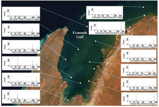
Figure 6.
Lomb–Scargle periodograms with x-axis showing TSM spectral frequencies (period in days) at 13 locations in the Exmouth Gulf; y-axis denotes Lomb–Scargle Power.
3.3. Metocean Drivers of Turbidity
3.3.1. Location Analyses
Time series analysis from 13 locations around the Gulf showed that there was interannual variability of turbidity at all sites (Figure 7a). The influence of ENSO at each of the 13 locations was seen in the time series (12-month rolling mean) for TSM, wave power, MSL, ENSO and IDM, where higher turbidity, sea level and wave power are apparent following strong ENSO (SOI index) events (Figure 7a–e). This influence was especially strong during the 2010/2011 extreme La Niña event.
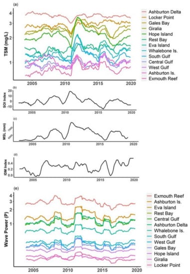
Figure 7.
The 12-month rolling mean of (a) turbidity (TSM) at 13 locations in the Exmouth Gulf; (b) El Niño-Southern Oscillation Index (SOI); (c) mean sea level, (d) Indian Ocean Dipole mode (IDM), and (e) wave power at 13 locations in the Exmouth Gulf.
Stepwise regression models and Pearson’s correlation analyses performed on the 13 time series locations reveal that drivers of turbidity varied in different regions of the Gulf (Figure 8; Table 1; full regression tables in Appendix A).
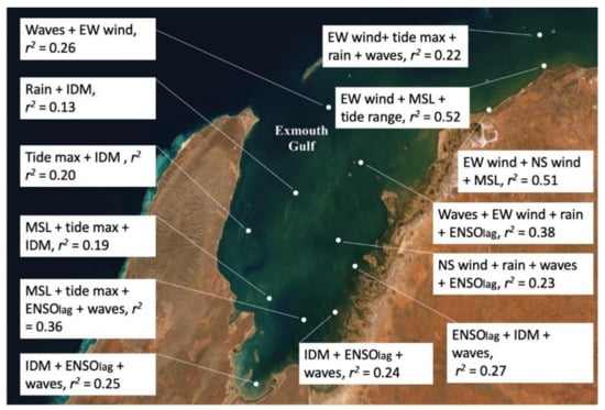
Figure 8.
Multiple regression results showing the metocean processes, east–west (EW) winds, north–south (NS) winds, mean sea level (MSL), tidal maxima, tidal range, rainfall, ENSO (10-month phase lag), wave power and Indian Ocean Diploe Mode (IDM), that best described turbidity at 13 locations in the Exmouth Gulf region between 2002 and 2019. Models were chosen by a backward stepwise regression process where the least significant variable was removed at each step and the best model chosen using the Akaike Information Criterion (AIC). Full regression table results available in Appendix A.

Table 1.
Pearson’s R correlation coefficients for (a) turbidity and environmental variables (wave power, east–west winds, north–south winds, tidal range (monthly average), tidal range (3-day average), tidal maximum, mean sea level, rainfall, Indian Ocean Dipole Mode (IDM) and El Niño–Southern Oscillation (ENSO) in the Exmouth Gulf. All correlations are from monthly averaged values except for 3-day tidal range. The R2 value was derived from multiple regression models using all variables (full stepwise regression table results in Appendix A); (b) correlations between waves and other environmental variables at 13 locations in the Exmouth Gulf and (c) correlations between all the environmental variables except waves.
Wind and waves were primary drivers of turbidity in the north and north-eastern regions of the Gulf. Waves also affected turbidity in the far south of the Gulf. For regions along the eastern and southern Gulf (Whalebone, South Gulf, Hope Is., Giralia, Gales Bay), ENSO (10-month lag phase) was a primary driver of turbidity, with the IDM (direct phase) also a primary driver at seven of the 13 locations. While monthly averaged tidal range was used in the regression analysis, only one location (Ashburton Island) contained this parameter in its turbidity model, however, the 3-day tidal range was significantly correlated to turbidity at multiple locations in the Pearson’s correlation analyses (Table 1). Mean sea level was a strongly correlated factor in some central, southern, and western locations (South Gulf, West Gulf, Whalebone Island) and rainfall was also correlated with turbidity in several locations (Eva Island, Central Gulf, Exmouth Reef, South Gulf, West Gulf, Whalebone Is.). Rainfall in the Gulf was strongly associated with increased winds and sea surface heights (tidal maxima, mean sea level; Table 1(b)), as well as waves (Table 1(c)) indicating that rainfall correlation with turbidity was strongly associated with these other drivers.
El Niño–Southern Oscillation and Indian Ocean Dipole
Correlations between turbidity and both ENSO and IOD varied with the different lag increments and at the different locations in the Gulf (Table A2 and Table A3). The eastern Gulf inshore locations were the most correlated to ENSO overall, with strongest correlations at 9–11 months lag. These same sites were also correlated (~30%) to the direct phase of the IOD. ENSO and IOD were also correlated significantly to each other at the 0–3-month lags and the 6–12-month lags, with a peak correlation at the 11-month lag (R = 0.277).
There was a significant effect of ENSO-IDM Phase type on turbidity at three locations inside the Exmouth Gulf: Hope Island, Whalebone Island and Gales Bay (Kruskal–Wallis p < 0.05). A Dunn’s test of multiple comparisons using rank sums showed that turbidity was significantly higher during a Type 4 Phase (ENSO positive, IOD positive) compared to a Type 3 Phase (ENSO Positive, IOD negative) at both Whalebone Island and Gales Bay (Table 2).
Table 2.
Effect of El Niño–Southern Oscillation and Indian Ocean Diploe phase combination on turbidity at two locations in the Exmouth Gulf.
3.3.2. Regional Analyses
Correlation maps between turbidity and environmental variables (east–west and north–south components of the wind, tidal range, tidal maximum, wave power, ENSO and IOD indexes, rainfall, and mean sea level), further supported the findings of the time series analyses and revealed larger-scale regional trends (Figure 9). Winds, waves, and sea level variability were highly correlated with turbidity, however, the effects differed throughout the Gulf. For example, higher turbidity in the northern Gulf was associated with winds from the east while turbidity in the southern Gulf was associated with winds from the west (Figure 9a). Wave power had a stronger influence in the north-east part of the Gulf than any other region, and in some parts of the southwest Gulf there was little effect of waves on turbidity. Rainfall had a high correlation with turbidity in the north-eastern Gulf (Figure 9i) and tidal maxima were highly correlated with turbidity in the southern Gulf regions (Figure 9c). Each correlation map has a corresponding p-value map where all significantly correlated (p < 0.05) pixels are coloured.
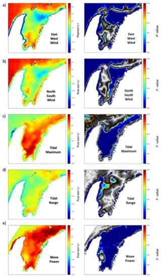
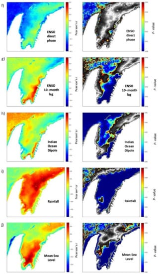
Figure 9.
Correlation maps showing the strength of the relationship at each pixel of the region (Pearson’s correlation coefficient R) and significance of the correlation (p-value) between mean monthly turbidity and (a) east–west winds (a negative R value denotes a correlation with easterly winds and a positive R correlates to westerly winds); (b) north–south winds (a negative R denotes correlation to northerly winds and a positive R to southerly winds); (c) tidal maximum; (d) tidal range; (e) wave power; (f) ENSO direct phase; (g) ENSO 10-month lag; (h) Indian Ocean Dipole; (i) rainfall; (j) mean sea level. Note: colour scale range may differ between plots.
Principal component analysis (PCA) resulted in three components that explained 87.6% of the data variance: 63.3% for PC1, 24.2% for PC2 and 0.07% for PC3 (Figure 10a–c). Both wind components (east–west and north–south) were the primary predictors of PC1; east–west wind, wave power, mean sea level and tidal maxima/ tidal range were the primary predictors of PC2, and wave power was primarily responsible for PC3 (Table 3).
Figure 10.
(a–c) Principal components 1, 2 and 3 (respectively) with overlay of nine geographical regions used to construct the biplot; (d) bi-plot showing the first two principal components that explain environmental drivers of turbidity from nine regions in the Exmouth Gulf. The cosine of the angles between the variable arrows estimates the correlations between the variables (from Table 3), the smaller the angle the higher the correlation. The length of arrows is roughly proportional to the standard deviation in the correlations for that variable, meaning that the longer the arrow, the more that variable is responsible for separating the groups.
Table 3.
Loadings from principal component analysis of metocean drivers of turbidity in the Exmouth Gulf.
Regions showing associations to the same principal component were grouped to give nine regional groups (the polygons were drawn where neighbouring pixels showed the same principal component associations (same colour) from all three principal component maps). The resulting regional groups show where environmental drivers of turbidity are similar within each region—NE Coast, East Coast and West Coast (inshore regions), and NE Gulf, North Gulf, Central Gulf, East Gulf and South Gulf (offshore regions; Figure 10a–c). When all data points within the grouped regions were plotted, the resulting bi-plot showed the clusters of these nine distinct geographic regions and their associated drivers of turbidity (Figure 10d). The bi-plot reveals that the environmental drivers ENSO (SOI), waves, sea surface height (tidal maxima and mean sea level) and rainfall were closely associated with each other, while east–west and north–south wind components were more independent of these other processes. Rainfall was highly associated with the negative phase of the Indian Dipole Mode and east–west winds were the main variable responsible for separating the regions, followed by north–south winds and mean sea level.
4. Discussion
4.1. Drivers of Spatial Variability in Turbidity
4.1.1. Northeast Coast
The highest turbidity in the Exmouth Gulf was found along the Gulf’s north-east coast (Locker Point, Ashburton Delta). Seasonality of turbidity was strong, with winter months experiencing the highest turbidity, coinciding with peaks in the easterly wind regime and rainfall patterns. This shallow coastline is highly exposed, particularly during easterly wind phases when long fetch can occur across this region of the North-West Shelf. These sites are also proximal to the mouth of the Ashburton River and therefore impacted by infrequent flood discharge events that occur primarily during cyclones [49]. Currents here are often tidally driven in an east–west orientation but become dominated by wind-driven flow during neap tides [63]. Wind forcing was the primary variable associated with high turbidity in this region, with correlations of r = 0.59–0.64 for easterly winds and r = 0.23–0.27 for northerly winds (both these directions provide large fetch to build wave energy). Many studies have shown the susceptibility of shallow coastal regions to resuspension of sediments, occurring under certain conditions of fetch, when wave induced shear-stress causes resuspension at the water–sediment interface [58,59,64]. Given a favourable fetch, the frequency and duration of wind forcing are often the most important factors driving turbidity in shallow water [59,64], however, wave induced sediment resuspension can vary according to sediment grain size and the presence/absence of benthic cover (i.e., seagrass) [65,66]. Sediments in this north-eastern region of the Gulf are clay-dominated and stay in suspension for extended periods [67], while seagrass/algal beds are sparse as well as deciduous and may not be stabilising sediments [49,68].
As well as driving wave-induced sediment resuspension, easterly winds are potentially depositing sediments via aeolian processes. Studies have shown the variation in clay mineral on the north-west shelf matches that of the adjacent soil crusts [67,69] and degradation of soil crusts adjacent to coasts is known to make significant contributions to marine ecosystem through aeolian dust deposition [70]. Pilbara soils are highly erodible [71] and it is known that during long dry periods, dust is transported to the shelf off north-western Australia by prevailing easterly to south-easterly trade winds [72]. Furthermore, dust storms in this region are known events, occurring 1–3 times annually associated with low pressure systems and cyclones/storms [73].
4.1.2. East Coast
The inshore regions along the eastern to south-eastern coastline of the Exmouth Gulf display the next highest average turbidity (after the north-east inshore coast). This coastline comprises complex, mangrove lined tidal channels with high silt/clay sediment content that is known to form muddy pools [67]. The strongest driver of turbidity along this coastline was the La Niña phase of ENSO (highest at the 10-month lag). It is known that this phase is also associated with increased sea level anomalies throughout the region as well as increased cyclonic and wave activity [74,75,76,77]. The positive phase of the Indian Ocean Dipole (pIOD) was also significantly correlated with turbidity along the inshore eastern coastline of the Gulf. The process by which this climate phenomenon is affecting this region is unclear despite several Indian Ocean basin wide studies on the effects of IOD variability, that have focussed on chlorophyll-a [78,79,80], biogeochemical responses [81] and even human infectious disease prevalence [82]. It is known from altimetry studies that pIOD reduces water levels in the eastern Indian Ocean south of Java by as much as 0.28 m [74] and lowers rainfall over inland Australia. Over the period of this study, pIOD was strongly correlated with reduced water heights, amplification in southerly winds, and lower rainfall in the Gulf. This combination of events may increase the susceptibility of these shallow regions to resuspension of sediments by wind/waves as found by others [58,59,64].
Turbidity in the eastern Gulf is also significantly associated with reduced tidal range at two locations (Gales Bay and Giralia). This is unexpected as reduced tidal range, such as during neap tidal phases, is often associated with a decrease in water turbidity due to weaker currents than those present during spring tide phases [83]. As with the shallow northeast coast, and the pIOD reduced water level effect previously mentioned, neap tides are potentially resulting in the seabed being within the range of sediment resuspension by locally generated wind waves while during spring tides the water level is too high for wind waves to resuspend sediments. Another potential mechanism is coastal trapping by haloclines, which are known to trap sediments [84,85,86] and are more likely to occur on neap tides when tidal range is lowest and salinity stratification is enhanced [87]. Salinity in the upper reaches of the Gulf can be 10% higher than that found in other parts of the Gulf [88]. This is consistent with findings in Gulf St Vincent, South Australia, where incoming tides during neap periods produced a strong salinity wedge while spring tides led to well mixed waters [89].
4.1.3. Body of Gulf
Exmouth Gulf is vast (~3000 km2) and turbidity is driven by combinations of metocean factors that differ in each defined region. Close to the mouth of the North Gulf region is Eva Island and Exmouth Reef, which are heavily exposed to NNW swell wave and southerly wind-wave energy. Island shoreline change on Eva Island is known to be sensitive to the metocean conditions that occur with ENSO, displaying an oscillating orientation of erosion–accretion that aligns with ENSO events [45]. Seasonal turbidity patterns in this region are like those in the NE Coast region, with higher turbidity occurring during winter months, coinciding with the winter intensification of easterly wind forcing and swell waves. Environmental variables correlating strongest with turbidity here were wave power, easterly winds, and rainfall. These findings are consistent with other regions, such as the inner shelf of the Great Barrier Reef, where wind driven waves were the major driver of turbidity [28,90], the Gulf of Mexico where wind and ENSO were primary drivers of turbidity [91], and an open coast in New Zealand where turbidity was primarily correlated with wave energy and rainfall [92]. It is likely that these turbidity drivers (higher water levels, wave power and rainfall) along with cyclones (due to the immense, but short-lived, wave power and winds) are the mechanism behind increased turbidity in the Gulf during La Niña phases of ENSO. We found many of these drivers (waves, rainfall, higher water levels) were intensified in the Exmouth Gulf region during the La Niña phase of ENSO (Figure 5) and this has been shown by others [45,77,93]. Furthermore, cyclonic activity is increased during La Niña phases in north Western Australia [94] and strong turbidity peaks are known to be associated with these events [47].
4.1.4. Central and East Gulf
Further south in the Central and East Gulf regions, the influence of the easterly wind on turbidity drops off dramatically. Wave energy is the primary driver of turbidity in both these regions, along with tidal influences, rainfall, and the IOD. The Central region is the deepest part of the Gulf (~15–21 m) and less susceptible to wind–wave-induced sediment resuspension, whilst also being far enough away from the coast that aeolian deposition of sediments is less likely as a regular occurrence. Limited resuspension due to depth has also been shown in New Zealand [92] and San Francisco [95], where deeper sites within channels did not show a turbidity response to local wind driven waves which have a much shorter wavelength compared to oceanic swells. The Central Gulf is also within the reach of the flood tide waters that draw in open ocean water between North West Cape and the Murion Islands and flush the western top-third of the Gulf [43]. The East Gulf is shallower (~8–10 m); unlike the Central Gulf, northerly winds as well as ENSO (at the 10-month lag), are additional drivers of turbidity here. Here, we also see a relationship between turbidity and the IOD, though less strong than the adjacent East Coast near shore regions.
4.1.5. West Gulf and Coast
The West Gulf and West Coast regions turbidity regime is highly influenced by north-easterly wind forcing, particularly the West Coast where this parameter’s influence is stronger than anywhere else in the Gulf. Like other shallow locations (Gales Bay, Giralia), turbidity on the West Coast was also strongly negatively correlated with neap tides. This contrasts with deeper offshore sites (West Gulf, South Gulf, Rest Bay, Eva Island) where higher monthly tidal range correlates to turbidity.
4.1.6. Southern Gulf
In the most southern reaches of the Gulf, metocean drivers of turbidity are like those found around the Central Gulf and East Gulf, where the pENSO effects of high water levels, rainfall and increased wave power are strongly associated with turbidity. Northerly winds are also correlated to turbidity here, potentially from the enhanced effect of fetch into the deeper parts of the Gulf. This region is also beyond the reach of the daily tidal flushing that enters the Gulf, and this may mean increased residence time of smaller particulates that are then subject to resuspension.
There is a small region around Rest Bay in the South-West Gulf, where wave power is not significantly correlated to turbidity. It is also the only region in the Gulf (apart from Giralia Bay) where south westerly winds are a stronger driver of turbidity than north easterly winds. Tidal influences and IOD are the only strong drivers of turbidity in this part of the Gulf.
4.2. Climate Change and Turbidity
This study has found pathways where climate change could alter turbidity regimes in Exmouth Gulf and negatively impact ecologically critical habitats. During the extreme La Niña event of 2010/2011 there was a corresponding large spike in turbidity in the Gulf, along with spikes in mean sea level and wave power (Figure 7). Climate change is expected to alter ENSO and IOD patterns and, while different outcomes have been modelled, the strong consensus is that both La Niña and El Niño extreme events will intensify [11,96]. As extreme pIOD events develop after, and are exacerbated by, extreme El Niño [62,97], it is expected that extreme pIOD events will also be a more frequent occurrence [98]. The frequency of extreme La Niña is also expected to increase in response to more extreme El Niños [99]. As well as being a strong driver of the metocean processes that are most strongly correlated to turbidity in the Gulf (wave power, sea level maxima, rainfall), extreme La Niña is associated with the marine heatwaves that lead to mass coral bleaching and destruction of benthic flora habitats [100,101,102]. Ecosystems already under stress from heatwaves could then be subjected to increased turbidity and may not recover to their same stable states. This has been shown previously in the Pilbara region where corals were slower to recover from bleaching events under turbid conditions [14].
These changing patterns could potentially trigger ecological impacts for parts of the Gulf including important coral reef systems, which are shown to be both productive and resilient to some turbidity fluctuation and temperature anomalies [103], as well as the eastern Gulf seagrass/macroalgal ecosystems. Here, we have shown that:
- Turbidity in the Exmouth Gulf has a strong relationship to ENSO and the synoptic influences that are driven by extreme La Niña phases.
- Turbidity in some Gulf habitats increases under pIOD events, meaning that more extreme pIOD (as predicted) could lead to more periods of higher turbidity.
- Wind, wave energy and sea level maxima are highly correlated to turbidity in many regions of the Gulf. Under climate change these processes are likely to increase, with more extreme La Niña and an increase in the frequency of the most intense cyclones.
- Extreme El Niño and extreme pIOD events are associated with drought conditions across Australia. The Pilbara Rangelands are a terrestrial source of aeolian sediment deposition in the Gulf, and with increased drought, there will be increased availability of loose sediments atop the soil crust, potentially leading to an increase in intensity of dust storms and turbidity during extreme wind events.
- Future work could attempt to quantify the climate change impacts to regional water quality by applying statistical methods that incorporate climate circulation models and emission scenarios [104] and machine learning approaches [105,106] to long-term hydrological data such as that presented in this study.
5. Conclusions
This study analysed 18 years of remotely sensed turbidity data from the Exmouth Gulf region of Western Australia to find the metocean processes that drive seasonal and interannual turbidity fluctuations in the Exmouth Gulf, north Western Australia. We find that while variability in turbidity is high, there has been a systematic upward trend in turbidity in some regions of the Gulf. The significant coupling of ENSO and IOD to turbidity reveals pathways where climate change could further impact water quality to ecologically critical habitats into the future. This highlights how important a better understanding of the relationship between global climate cycles, regional oceanographic processes and turbidity is to the future management of coastal environmental values under the influence of climate change. This study was limited to the quantification of turbidity variability and its associated metocean processes. We recommend that future studies should approach the quantification of climate change impacts to water quality variability by using long term hydrological data (such as we have produced in this work) and applying novel statistical approaches that incorporate climate change circulation models and emission scenarios.
Author Contributions
P.J.C. conceived the study, contributed to image analysis and processing, and analysed all results. P.R.C.S.F. adapted the turbidity algorithm and contributed to image analysis and processing. P.B. and M.V.W.C. developed the numerical wave-circulation model and conducted the 20-year wave hindcast. M.O. contributed to study design and data interpretation. N.K.B. contributed to study design and data interpretation. R.J.L. contributed to method development. All authors contributed to the manuscript. All authors have read and agreed to the published version of the manuscript.
Funding
P.J.C. was supported by an Australian Research Training Scholarship.
Acknowledgments
The authors would like to thank the National Aeronautics and Space Administration (NASA) for supplying open access satellite data to the scientific community. This work was supported by resources provided by the Pawsey Supercomputing Centre. We also thank the Department of Transport, Western Australia, for supplying tide data and the Australian Bureau of Meteorology for supplying the rainfall data.
Conflicts of Interest
The authors declare no conflict of interest. The funders had no role in the design of the study; in the collection, analyses, or interpretation of data; in the writing of the manuscript, or in the decision to publish the results.
Appendix A
Table A1.
Modified Mann–Kendall table of results.
Table A1.
Modified Mann–Kendall table of results.
| Location | Corrected Zc | Tau | New p-Value | Sens Slope | Trend |
|---|---|---|---|---|---|
| Ashburton D. | −2.674 | −0.059 | 0.008 | −0.0002 | Decreasing |
| Locker Pt. | 1.723 | 0.042 | 0.084 | 0.00019 | No sig. trend |
| Gales | 0.730 | 0.032 | 0.465 | 0.00005 | No sig. trend |
| Giralia | 0.636 | 0.034 | 0.524 | 0.00004 | No sig. trend |
| Hope | 0.251 | 0.011 | 0.801 | 0.00001 | No sig. trend |
| Eva Is. | 1.716 | 0.017 | 0.003 | 0.000004 | Increasing |
| Central Gulf | 1.652 | 0.016 | 0.102 | 0.000007 | No sig. trend |
| South Gulf | 1.256 | 0.045 | 0.208 | 0.00002 | No sig. trend |
| West Gulf | 4.599 | 0.056 | <0.0001 | 0.00002 | Increasing |
| Whalebone | 2.646 | 0.065 | 0.008 | 0.00003 | Increasing |
| Rest | 1.732 | 0.052 | 0.083 | 0.00004 | No sig. trend |
| Ashburton Is. | −0.706 | −0.031 | 0.480 | −0.00002 | Ni sig. trend |
| Exmouth Reef | 1.716 | 0.086 | 0.086 | 0.00002 | No sig. trend |
Table A2.
Pearson’s r correlations between turbidity and the El-Niño Southern Oscillation Index (SOI) at different time lags. Highlighted cells indicate significant correlations (p < 0.05). Additionally included is the correlation between SOI and the Indian Dipole Mode (IDM) at the same lag increments.
| Location | SOI + 0 | SOI + 1 | SOI + 2 | SOI + 3 | SOI + 4 | SOI + 5 | SOI + 6 | SOI + 7 | SOI + 8 | SOI + 9 | SOI + 10 | SOI + 11 | SOI + 12 |
|---|---|---|---|---|---|---|---|---|---|---|---|---|---|
| Ashburton Delta | −0.123 | −0.134 | −0.035 | −0.084 | 0.044 | 0.097 | 0.104 | 0.099 | 0.171 | 0.085 | 0.034 | 0.009 | −0.059 |
| Gales Bay | 0.101 | 0.161 | 0.201 | 0.197 | 0.228 | 0.302 | 0.353 | 0.348 | 0.397 | 0.406 | 0.373 | 0.425 | 0.286 |
| Giralia | 0.077 | 0.142 | 0.119 | 0.137 | 0.167 | 0.266 | 0.331 | 0.324 | 0.38 | 0.386 | 0.374 | 0.361 | 0.267 |
| Hope Is | 0.175 | 0.199 | 0.237 | 0.216 | 0.293 | 0.367 | 0.417 | 0.425 | 0.451 | 0.436 | 0.45 | 0.372 | 0.324 |
| Central Gulf | −0.05 | −0.026 | 0.004 | −0.087 | −0.073 | 0.042 | −0.002 | 0.003 | 0.008 | 0.038 | 0.096 | −0.001 | 0.025 |
| Eva | 0.021 | 0.071 | 0.139 | 0.06 | 0.144 | 0.243 | 0.179 | 0.203 | 0.147 | 0.136 | 0.147 | 0.015 | 0.023 |
| Rest Bay | 0.046 | −0.049 | −0.052 | −0.157 | −0.119 | −0.048 | −0.036 | −0.046 | 0.004 | 0.036 | 0.105 | 0.052 | 0.09 |
| Exmouth Reef | −0.001 | 0.089 | 0.124 | 0.095 | 0.182 | 0.24 | 0.21 | 0.222 | 0.166 | 0.166 | 0.194 | 0.057 | 0.028 |
| Open Water | −0.15 | −0.103 | −0.083 | −0.141 | −0.057 | 0.061 | 0.015 | 0.087 | 0.092 | 0.087 | 0.128 | 0.119 | 0.161 |
| Ashburton Is | 0.079 | 0.026 | 0.042 | −0.069 | −0.068 | −0.08 | −0.13 | −0.125 | −0.117 | −0.17 | −0.071 | −0.154 | −0.068 |
| IDM | −0.124 | −0.142 | −0.201 | −0.1 | 0.004 | 0.081 | 0.167 | 0.255 | 0.291 | 0.266 | 0.255 | 0.277 | 0.208 |
Table A3.
Pearson’s r correlations between turbidity and the Indian Ocean Dipole mode (IDM) at different time lags. Highlighted cells indicate significant correlations (p < 0.05).
Table A3.
Pearson’s r correlations between turbidity and the Indian Ocean Dipole mode (IDM) at different time lags. Highlighted cells indicate significant correlations (p < 0.05).
| Location | IDM + 0 | IDM + 1 | IDM + 2 | IDM + 3 | IDM + 4 | IDM + 5 | IDM + 6 | IDM + 7 | IDM + 8 | IDM + 9 | IDM + 10 | IDM + 11 | IDM + 12 |
|---|---|---|---|---|---|---|---|---|---|---|---|---|---|
| Ashburton Delta | 0.042 | −0.021 | −0.145 | −0.279 | −0.283 | −0.175 | −0.132 | −0.04 | 0.012 | 0.143 | 0.209 | 0.195 | 0.107 |
| Gales Bay | 0.319 | 0.27 | 0.189 | 0.073 | 0.021 | 0.054 | −0.022 | −0.05 | −0.032 | −0.003 | 0.079 | 0.139 | 0.187 |
| Giralia | 0.297 | 0.252 | 0.159 | 0.031 | −0.053 | −0.048 | −0.09 | −0.117 | −0.101 | −0.057 | 0.023 | 0.101 | 0.176 |
| Hope Is | 0.249 | 0.22 | 0.141 | 0.052 | −0.009 | 0.017 | −0.035 | −0.068 | −0.071 | −0.047 | 0.015 | 0.071 | 0.131 |
| Central Gulf | 0.15 | 0.131 | 0.036 | −0.018 | −0.001 | 0.092 | 0.1 | 0.092 | −0.01 | 0.006 | 0.062 | 0.068 | 0.042 |
| Eva | 0.078 | 0.024 | −0.056 | −0.094 | −0.057 | 0.037 | 0.084 | 0.067 | 0.09 | 0.192 | 0.219 | 0.138 | 0.027 |
| Rest Bay | 0.119 | 0.175 | 0.183 | 0.102 | 0.127 | 0.265 | 0.25 | 0.192 | 0.017 | −0.053 | −0.063 | −0.092 | −0.089 |
| Exmouth Reef | 0.17 | 0.065 | −0.058 | −0.155 | −0.16 | −0.062 | 0 | 0.027 | 0.017 | 0.108 | 0.214 | 0.211 | 0.162 |
| Open Water | 0.308 | 0.249 | 0.191 | 0.05 | −0.02 | −0.015 | −0.021 | −0.03 | −0.57 | −0.047 | 0.02 | 0.104 | 0.143 |
| Ashburton Is | 0 | −0.017 | −0.053 | −0.007 | −0.047 | 0.118 | 0.122 | −0.021 | −0.115 | −0.095 | −0.074 | −0.036 | −0.063 |
References
- Halpern, B.S.; Walbridge, S.; Selkoe, K.A.; Kappel, C.V.; Micheli, F.; D’Agrosa, C.; Bruno, J.F.; Casey, K.S.; Ebert, C.; Fox, H.E.; et al. A Global Map of Human Impact on Marine Ecosystems. Science 2008, 319, 948–952. [Google Scholar] [CrossRef]
- Crain, C.M.; Halpern, B.S.; Beck, M.W.; Kappel, C.V. Understanding and managing human threats to the coastal marine environment. Ann. N. Y. Acad. Sci. 2009, 1162, 39–62. [Google Scholar] [CrossRef]
- Duarte, C.M.; Dennison, W.C.; Orth, R.J.W.; Carruthers, T.J.B. The Charisma of Coastal Ecosystems: Addressing the Imbalance. Estuar. Coasts 2008, 31, 233–238. [Google Scholar] [CrossRef]
- Lu, Y.; Yuan, J.; Lu, X.; Su, C.; Zhang, Y.; Wang, C.; Cao, X.; Li, Q.; Su, J.; Ittekkot, V.; et al. Major threats of pollution and climate change to global coastal ecosystems and enhanced management for sustainability. Environ. Pollut. 2018, 239, 670–680. [Google Scholar] [CrossRef] [PubMed]
- Rathore, S.; Bindoff, N.L.; Phillips, H.E.; Feng, M. Recent hemispheric asymmetry in global ocean warming induced by climate change and internal variability. Nat. Commun. 2020, 11, 2008. [Google Scholar] [CrossRef]
- Dove, S.G.; Kline, D.I.; Pantos, O.; Angly, F.E.; Tyson, G.W.; Hoegh-Guldberg, O. Future reef decalcification under a business-as-usual CO(2) emission scenario. Proc. Natl. Acad. Sci. USA 2013, 110, 15342–15347. [Google Scholar] [CrossRef] [PubMed]
- Sydeman, W.J.; García-Reyes, M.; Schoeman, D.S.; Rykaczewski, R.R.; Thompson, S.A.; Black, B.A.; Bograd, S.J. Climate change and wind intensification in coastal upwelling ecosystems. Science 2014, 345, 77. [Google Scholar] [CrossRef]
- Knutson, T.R.; McBride, J.L.; Chan, J.; Emanuel, K.; Holland, G.; Landsea, C.; Held, I.; Kossin, J.P.; Srivastava, A.K.; Sugi, M. Tropical cyclones and climate change. Nat. Geosci. 2010, 3, 157–163. [Google Scholar] [CrossRef]
- Dobrynin, M.; Murawski, J.; Baehr, J.; Ilyina, T. Detection and Attribution of Climate Change Signal in Ocean Wind Waves. J. Clim. 2015, 28, 1578–1591. [Google Scholar] [CrossRef]
- Chen, X.; Zhang, X.; Church, J.A.; Watson, C.S.; King, M.A.; Monselesan, D.; Legresy, B.; Harig, C. The increasing rate of global mean sea-level rise during 1993–2014. Nat. Clim. Chang. 2017, 7, 492–495. [Google Scholar] [CrossRef]
- Ham, Y.-G. El Niño events will intensify under global warming. Nature 2018, 564, 192–193. [Google Scholar] [CrossRef] [PubMed]
- Zhou, Z.-Q.; Xie, S.-P.; Zheng, X.-T.; Liu, Q. Indian Ocean Dipole response to global warming: A multi-member study with CCSM4. J. Ocean Univ. China 2013, 12, 209–215. [Google Scholar] [CrossRef]
- Cai, W.; Wang, G.; Dewitte, B.; Wu, L.; Santoso, A.; Takahashi, K.; Yang, Y.; Carréric, A.; McPhaden, M.J. Increased variability of eastern Pacific El Niño under greenhouse warming. Nature 2018, 564, 201. [Google Scholar] [CrossRef]
- Evans, R.D.; Wilson, S.K.; Fisher, R.; Ryan, N.M.; Babcock, R.; Blakeway, D.; Bond, T.; Dorji, P.; Dufois, F.; Fearns, P.; et al. Early recovery dynamics of turbid coral reefs after recurring bleaching events. J. Environ. Manag. 2020, 268, 110666. [Google Scholar] [CrossRef]
- Kirk, J.T. Light and Photosynthesis in Aquatic Ecosystems; Cambridge University Press: Cambridge, UK, 1994. [Google Scholar]
- Erftemeijer, P.L.; Riegl, B.; Hoeksema, B.W.; Todd, P.A. Environmental impacts of dredging and other sediment disturbances on corals: A review. Mar. Pollut. Bull. 2012, 64, 1737–1765. [Google Scholar] [CrossRef] [PubMed]
- Post, A.L.; Wassenberg, T.J.; Passlow, V. Physical surrogates for macrofaunal distributions and abundance in a tropical gulf. Mar. Fresh. Res. 2006, 57, 469–483. [Google Scholar] [CrossRef]
- Fabricius, K.E. Effects of terrestrial runoff on the ecology of corals and coral reefs: Review and synthesis. Mar. Pollut. Bull. 2005, 50, 125–146. [Google Scholar] [CrossRef] [PubMed]
- Weber, M.; Lott, C.; Fabricius, K.E. Sedimentation stress in a scleractinian coral exposed to terrestrial and marine sediments with contrasting physical, organic and geochemical properties. J. Exp. Mar. Biol. Ecol. 2006, 336, 18–32. [Google Scholar] [CrossRef]
- Fisher, R.; Bessell-Browne, P.; Jones, R. Synergistic and antagonistic impacts of suspended sediments and thermal stress on corals. Nat. Comm. 2019, 10, 2346. [Google Scholar] [CrossRef]
- Bendix, J.; Wiley, J.J.; Commons, M.G. Intermediate disturbance and patterns of species richness. Phys. Geogr. 2017, 38, 393–403. [Google Scholar] [CrossRef]
- Morgan, K.M.; Perry, C.T.; Johnson, J.A.; Smithers, S.G. Nearshore Turbid-Zone Corals Exhibit High Bleaching Tolerance on the Great Barrier Reef Following the 2016 Ocean Warming Event. Front. Mar. Sci. 2017, 4. [Google Scholar] [CrossRef]
- Jordán-Garza, A.G.; González-Gándara, C.; Salas-Pérez, J.J.; Morales-Barragan, A.M. Coral assemblages are structured along a turbidity gradient on the Southwestern Gulf of Mexico, Veracruz. Cont. Shelf Res. 2017, 138, 32–40. [Google Scholar] [CrossRef]
- Zweifler, A.; O’Leary, M.; Morgan, K.; Browne, N.K. Turbid Coral Reefs: Past, Present and Future—A Review. Diversity 2021, 13, 251. [Google Scholar] [CrossRef]
- Larcombe, P.; Carter, R. Cyclone pumping, sediment partitioning and the development of the Great Barrier Reef shelf system: A review. Quat. Sci. Rev. 2004, 23, 107–135. [Google Scholar] [CrossRef]
- Anthony, K.R.N.; Ridd, P.V.; Orpin, A.R.; Larcombe, P.; Lough, J. Temporal variation of light availability in coastal benthic habitats: Effects of clouds, turbidity, and tides. Limnol. Oceanogr. 2004, 49, 2201–2211. [Google Scholar] [CrossRef]
- Van Senden, D.; Taylor, D.; Branson, P. Realtime turbidity monitoring and modelling for dredge impact assessment in Darwin Harbour. In Proceedings of the 14th Australasian Port and Harbour Conference, Sydney, Australia, 11–13 September 2013. [Google Scholar]
- Browne, N.; Smithers, S.; Perry, C. Spatial and temporal variations in turbidity on two inshore turbid reefs on the Great Barrier Reef, Australia. Coral Reefs 2013, 32, 195–210. [Google Scholar] [CrossRef]
- Barnard, P.L.; Hoover, D.; Hubbard, D.M.; Snyder, A.; Ludka, B.C.; Allan, J.; Kaminsky, G.M.; Ruggiero, P.; Gallien, T.W.; Gabel, L. Extreme oceanographic forcing and coastal response due to the 2015–2016 El Niño. Nature Commun. 2017, 8, 1–8. [Google Scholar] [CrossRef] [PubMed]
- Fearns, P.; Greenwood, J.; Chedzey, H.; Dorji, P.; Broomhall, M.; King, E.; Cherukuru, N.; Hardman-Mountford, N.; Antoine, D. Remote Sensing for Environmental Monitoring and Management in the Kimberley. Final. Rep. Project 2017, 1. Available online: http://hdl.handle.net/102.100.100/87570?index=1 (accessed on 11 February 2019).
- Hedley, J.; Roelfsema, C.; Chollett, I.; Harborne, A.; Heron, S.; Weeks, S.; Skirving, W.; Strong, A.; Eakin, C.; Christensen, T. Remote sensing of coral reefs for monitoring and management: A review. Remote Sens. 2016, 8, 118. [Google Scholar] [CrossRef]
- Gholizadeh, M.H.; Melesse, A.M.; Reddi, L. A Comprehensive Review on Water Quality Parameters Estimation Using Remote Sensing Techniques. Sensors 2016, 16, 1298. [Google Scholar] [CrossRef]
- Dorji, P.; Fearns, P. A Quantitative Comparison of Total Suspended Sediment Algorithms: A Case Study of the Last Decade for MODIS and Landsat-Based Sensors. Remote Sens. 2016, 8, 810. [Google Scholar] [CrossRef]
- Wulder, M.A.; Loveland, T.R.; Roy, D.P.; Crawford, C.J.; Masek, J.G.; Woodcock, C.E.; Allen, R.G.; Anderson, M.C.; Belward, A.S.; Cohen, W.B. Current status of Landsat program, science, and applications. Remote Sens. Environ. 2019, 225, 127–147. [Google Scholar] [CrossRef]
- NASA. NASA Goddard Space Flight Center, Ocean Ecology Laboratory, Ocean Biology Processing Group. In Moderate-Resolution Imaging Spectroradiometer (MODIS) Aqua Data; AOB.DAAC: Greenbelt, MD, USA. Available online: https://oceancolor.gsfc.nasa.gov/cgi/browse.pl?sen=am (accessed on 11 February 2019).
- Oceanica. Marine and Coastal Environment of the Eastern Exmouth Gulf. Available online: https://www.epa.wa.gov.au/sites/default/files/PER_documentation/1295-ERMP-Appendix%207-Marine%20and%20coastal%20environment%20V1-2.pdf2006; (accessed on 11 February 2019).
- Preen, A.R.; Marsh, H.; Lawler, I.R.; Prince, R.I.T.; Shepherd, R. Distribution and Abundance of Dugongs, Turtles, Dolphins and other Megafauna in Shark Bay, Ningaloo Reef and Exmouth Gulf, Western Australia. Wildl. Res. 1997, 24, 185–208. [Google Scholar] [CrossRef]
- Williamson, D.; Hamilton-Smith, E. Cape range and ningaloo reef: A semi-arid karst and coastal area unlike any other. Australasian Cave Karst Manag. 2009, 18, 78–93. [Google Scholar]
- Martín, J.; Puig, P.; Palanques, A.; Giamportone, A. Commercial bottom trawling as a driver of sediment dynamics and deep seascape evolution in the Anthropocene. Anthropocene 2014, 7, 1–15. [Google Scholar] [CrossRef]
- Haslam Mckenzie, F. Delivering enduring benefits from a gas development: Governance and planning challenges in remote Western Australia. Aust. Geogr. 2013, 44, 341–358. [Google Scholar] [CrossRef]
- Chapman, R.; Tonts, M.; Plummer, P. Resource development, local adjustment, and regional policy: Resolving the problem of rapid growth in the Pilbara, Western Australia. J. Rural Dev. 2014, 9, 72–86. [Google Scholar]
- EPA. Potential Cumulative Impacts of the Activities and Developments Proposed for Exmouth Gulf. 2021. Available online: https://www.epa.wa.gov.au/potential-cumulative-impacts-activities-and-developments-proposed-exmouth-gulf (accessed on 20 August 2021).
- Massel, S.; Brickman, R.; Mason, L.; Bode, L. Water circulation and waves in Exmouth Gulf. In Proceedings of the Australian Physical Oceanography Conference, Sydney, Australia; 1997; p. 48. [Google Scholar]
- Semeniuk, V. Development of mangrove habitats along ria shorelines in north and northwestern tropical Australia. Vegetatio 1985, 60, 3–23. [Google Scholar] [CrossRef]
- Cuttler, M.V.; Vos, K.; Branson, P.; Hansen, J.E.; O’Leary, M.; Browne, N.K.; Lowe, R.J. Interannual Response of Reef Islands to Climate-Driven Variations in Water Level and Wave Climate. Remote Sens. 2020, 12, 4089. [Google Scholar] [CrossRef]
- Lovelock, C.E.; Grinham, A.; Adame, M.F.; Penrose, H.M. Elemental composition and productivity of cyanobacterial mats in an arid zone estuary in north Western Australia. Wetl. Ecol. Manag. 2010, 18, 37–47. [Google Scholar] [CrossRef]
- Dufois, F.; Lowe, R.J.; Branson, P.; Fearns, P. Tropical Cyclone-Driven Sediment Dynamics Over the Australian North West Shelf. J. Geophys. Res. Oceans 2017, 122, 10225–10244. [Google Scholar] [CrossRef]
- Liu, K.S.; Chan, J.C. Interannual variation of Southern Hemisphere tropical cyclone activity and seasonal forecast of tropical cyclone number in the Australian region. Int. J. Climatol. 2012, 32, 190–202. [Google Scholar] [CrossRef]
- Loneragan, N.; Kangas, M.; Haywood, M.; Kenyon, R.; Caputi, N.; Sporer, E. Impact of cyclones and aquatic macrophytes on recruitment and landings of tiger prawns Penaeus esculentus in Exmouth Gulf, Western Australia. Estaur. Coast. Shelf 2013, 127, 46–58. [Google Scholar] [CrossRef]
- Ruddick, K.G.; Ovidio, F.; Rijkeboer, M. Atmospheric correction of SeaWiFS imagery for turbid coastal and inland waters. Appl. Opt. 2000, 39, 897–912. [Google Scholar] [CrossRef]
- Dorji, P.; Fearns, P.; Broomhall, M. A Semi-Analytic Model for Estimating Total Suspended Sediment Concentration in Turbid Coastal Waters of Northern Western Australia Using MODIS-Aqua 250 m Data. Remote Sens. 2016, 8. [Google Scholar] [CrossRef]
- Hamed, K.H.; Rao, A. A modified Mann-Kendall trend test for autocorrelated data. J. Hydrol. 1998, 204, 182–196. [Google Scholar] [CrossRef]
- RStudio. Integrated Development for R; PBC: Boston, MA, USA, 2020. [Google Scholar]
- Ruf, T. The Lomb-Scargle periodogram in biological rhythm research: Analysis of incomplete and unequally spaced time-series. Biol. Rhyth. Res. 1999, 30, 178–201. [Google Scholar] [CrossRef]
- VanderPlas, J.T. Understanding the lomb–scargle periodogram. Astrophys. J. Suppl. Ser. 2018, 236, 16. [Google Scholar] [CrossRef]
- Akaike, H. Factor analysis and AIC. In Selected Papers of Hirotugu Akaike; Springer: Berlin/Heidelberg, Germany, 1987; pp. 371–386. [Google Scholar]
- Branson, P.M.; Sun, C. Wamsi dredging science node: Plume modelling uncertainty-hydrodynamics. In Proceedings of the Coasts & Ports 2017 Conference, Cairns, Australia, 21–23 June 2017; p. 159. [Google Scholar]
- Arfi, R.; Guiral, D.; Bouvy, M. Wind induced resuspension in a shallow tropical lagoon. Estuar. Coast. Shelf 1993, 36, 587–604. [Google Scholar] [CrossRef]
- Booth, J.; Miller, R.; McKee, B.; Leathers, R. Wind-induced bottom sediment resuspension in a microtidal coastal environment. Cont. Shelf Res. 2000, 20, 785–806. [Google Scholar] [CrossRef]
- Philander, S.; Yamagata, T.; Pacanowski, R. Unstable air-sea interactions in the tropics. J. Atmosph. Sci. 1984, 41, 604–613. [Google Scholar] [CrossRef]
- Kug, J.-S.; Kang, I.-S. Interactive feedback between ENSO and the Indian Ocean. J. Clim. 2006, 19, 1784–1801. [Google Scholar] [CrossRef]
- Wang, H.; Kumar, A.; Murtugudde, R.; Narapusetty, B.; Seip, K.L. Covariations between the Indian Ocean dipole and ENSO: A modeling study. Clim. Dyn. 2019, 53, 5743–5761. [Google Scholar] [CrossRef]
- Condie, S.A.; Andrewartha, J.R. Circulation and connectivity on the Australian North West Shelf. Cont. Shelf Res. 2008, 28, 1724–1739. [Google Scholar] [CrossRef]
- Bailey, M.C.; Hamilton, D.P. Wind induced sediment resuspension: A lake-wide model. Ecol. Model. 1997, 99, 217–228. [Google Scholar] [CrossRef]
- Larsen, L.H.; Sternberg, R.W.; Shi, N.C.; Marsden, M.A.H.; Thomas, L. Field investigations of the threshold of grain motion by ocean waves and currents. Mar. Geol. 1981, 42, 105–132. [Google Scholar] [CrossRef]
- Ward, L.G.; Michael Kemp, W.; Boynton, W.R. The influence of waves and seagrass communities on suspended particulates in an estuarine embayment. Mar. Geol. 1984, 59, 85–103. [Google Scholar] [CrossRef]
- Brunskill, G.; Orpin, A.; Zagorskis, I.; Woolfe, K.; Ellison, J. Geochemistry and particle size of surface sediments of Exmouth Gulf, Northwest Shelf, Australia. Cont. Shelf Res. 2001, 21, 157–201. [Google Scholar] [CrossRef]
- McCook, L.; Klumpp, D.; McKinnon, A. Seagrass communities in Exmouth Gulf, Western Australia: A preliminary survey. J. R. Soc. West. Aust. 1995, 78, 81–87. [Google Scholar]
- Gingele, F.X.; De Deckker, P.; Hillenbrand, C.-D. Clay mineral distribution in surface sediments between Indonesia and NW Australia—Source and transport by ocean currents. Mar. Geol. 2001, 179, 135–146. [Google Scholar] [CrossRef]
- McTainsh, G.; Strong, C. The role of aeolian dust in ecosystems. Geomorphology 2007, 89, 39–54. [Google Scholar] [CrossRef]
- Smith, J.; Sullivan, L. Construction and maintenance of embankments using highly erodible soils in the Pilbara, North-Western Australia. Int. J. Geomate 2014, 6, 897–902. [Google Scholar] [CrossRef]
- Bowler, J.M. Aridity in Australia: Age, origins and expression in aeolian landforms and sediments. Earth Sci. Rev. 1976, 12, 279–310. [Google Scholar] [CrossRef]
- McTainsh, G.; O’Loingsigh, T.; Strong, C. Update of Dust Storm Index (DSI) Maps for 2005 to 2010; Atmospheric Environment Research Centre, Griffith University: Brisbane, Queensland, 2011. [Google Scholar]
- Fadlan, A.; Sugianto, D.N.; Zainuri, M. Influence of ENSO and IOD to Variability of Sea Surface Height in the North and South of Java Island. In Proceedings of the IOP Conference Series: Earth and Environmental Science, Shanghai, China, 19–22 October 2017; p. 012021. [Google Scholar]
- Amin, M. Changing mean sea level and tidal constants on the west coast of Australia. Mar. Fresh. Res. 1993, 44, 911–925. [Google Scholar] [CrossRef]
- Dufois, F.; Lowe, R.J.; Rayson, M.D.; Branson, P.M. A numerical study of tropical cyclone-induced sediment dynamics on the Australian North West Shelf. J. Geophys. Res. Oceans 2018, 123, 5113–5133. [Google Scholar] [CrossRef]
- Lowe, R.J.; Cuttler, M.V.; Hansen, J.E. Climatic drivers of extreme sea level events along the coastline of Western Australia. Earth’s Future 2021. [Google Scholar]
- Park, J.-Y.; Kug, J.-S. Marine biological feedback associated with Indian Ocean Dipole in a coupled ocean/biogeochemical model. Clim. Dyn. 2014, 42, 329–343. [Google Scholar] [CrossRef]
- Pandey, S.; Bhagawati, C.; Dandapat, S.; Chakraborty, A. Surface chlorophyll anomalies associated with Indian Ocean Dipole and El Niño Southern Oscillation in North Indian Ocean: A case study of 2006–2007 event. Environ. Monit. Assess. 2019, 191, 1–14. [Google Scholar] [CrossRef]
- Thushara, V.; Vinayachandran, P. Unprecedented surface chlorophyll blooms in the southeastern Arabian Sea during an extreme negative Indian Ocean Dipole. Geophys. Res. Lett. 2020, 47, e2019GL085026. [Google Scholar] [CrossRef]
- Wiggert, J.D.; Vialard, J.; Behrenfeld, M.J. Basinwide modification of dynamical and biogeochemical processes by the positive phase of the Indian Ocean Dipole during the SeaWiFS era. Geophys. Monogr. Ser. 2009, 185, 350. [Google Scholar]
- Lal, A.; Hashizume, M.; Hales, S. Indian Ocean Dipole and Cryptosporidiosis in Australia: Short-Term and Nonlinear Associations. Environ. Sci. Technol. 2017, 51, 8119–8127. [Google Scholar] [CrossRef]
- Kleypas, J. Coral reef development under naturally turbid conditions: Fringing reefs near Broad Sound, Australia. Coral Reefs 1996, 15, 153–167. [Google Scholar] [CrossRef]
- Burchard, H.; Baumert, H. The formation of estuarine turbidity maxima due to density effects in the salt wedge. A hydrodynamic process study. J. Phys. Oceanogr. 1998, 28, 309–321. [Google Scholar] [CrossRef]
- Geyer, W.R. The importance of suppression of turbulence by stratification on the estuarine turbidity maximum. Estuaries 1993, 16, 113–125. [Google Scholar] [CrossRef]
- Yellen, B.; Woodruff, J.D.; Ralston, D.K.; MacDonald, D.G.; Jones, D.S. Salt wedge dynamics lead to enhanced sediment trapping within side embayments in high-energy estuaries. J. Geophys. Res. Oceans 2017, 122, 2226–2242. [Google Scholar] [CrossRef]
- Ren, J.; Wu, J. Sediment trapping by haloclines of a river plume in the Pearl River Estuary. Cont. Shelf Res. 2014, 82, 1–8. [Google Scholar] [CrossRef]
- McKinnon, A.; Ayukai, T. Copepod egg production and food resources in Exmouth Gulf, Western Australia. Mar. Fresh. Res. 1996, 47, 595–603. [Google Scholar] [CrossRef]
- De Silva Samarasinghe, J.R.; Lennon, G.W. Hypersalinity, flushing and transient salt-wedges in a tidal gulf—An inverse estuary. Estuar. Coast. Shelf 1987, 24, 483–498. [Google Scholar] [CrossRef]
- Orpin, A.R.; Ridd, P.V.; Thomas, S.; Anthony, K.R.; Marshall, P.; Oliver, J. Natural turbidity variability and weather forecasts in risk management of anthropogenic sediment discharge near sensitive environments. Mar. Pollut. Bull. 2004, 49, 602–612. [Google Scholar] [CrossRef]
- McCarthy, M.J.; Otis, D.B.; Méndez-Lázaro, P.; Muller-Karger, F.E. Water Quality Drivers in 11 Gulf of Mexico Estuaries. Remote Sens. 2018, 10, 255. [Google Scholar] [CrossRef]
- Seers, B.M.; Shears, N.T. Spatio-temporal patterns in coastal turbidity–long-term trends and drivers of variation across an estuarine-open coast gradient. Estuar. Coast. Shelf 2015, 154, 137–151. [Google Scholar] [CrossRef]
- Pattiaratchi, C.; Buchan, S.J. Implications of long-term climate change for the Leeuwin Current. J. R. Soc. West. Aust 1991, 74, 133–140. [Google Scholar]
- Goebbert, K.H.; Leslie, L.M. Interannual variability of northwest Australian tropical cyclones. J. Clim. 2010, 23, 4538–4555. [Google Scholar] [CrossRef][Green Version]
- Ruhl, C.; Schoellhamer, D.; Stumpf, R.; Lindsay, C. Combined use of remote sensing and continuous monitoring to analyse the variability of suspended-sediment concentrations in San Francisco Bay, California. Estuar. Coast. Shelf 2001, 53, 801–812. [Google Scholar] [CrossRef]
- Cai, W.; Wu, L.; Lengaigne, M.; Li, T.; Mcgregor, S.; Kug, J.-S.; Yu, J.-Y.; Stuecker, M.F.; Santoso, A.; Li, X. Pantropical climate interactions. Science 2019, 363, eaav4236. [Google Scholar] [CrossRef]
- Cai, W.; Wang, G.; Gan, B.; Wu, L.; Santoso, A.; Lin, X.; Chen, Z.; Jia, F.; Yamagata, T. Stabilised frequency of extreme positive Indian Ocean Dipole under 1.5 C warming. Nat. Comm. 2018, 9, 1419. [Google Scholar] [CrossRef]
- Wang, G.; Cai, W.; Yang, K.; Santoso, A.; Yamagata, T. A unique feature of the 2019 extreme positive Indian Ocean Dipole event. Geophys. Res. Lett. 2020, 47, e2020GL088615. [Google Scholar] [CrossRef]
- Cai, W.; Santoso, A.; Wang, G.; Yeh, S.-W.; An, S.-I.; Cobb, K.M.; Collins, M.; Guilyardi, E.; Jin, F.-F.; Kug, J.-S.; et al. ENSO and greenhouse warming. Nat. Clim. Change 2015, 5, 849–859. [Google Scholar] [CrossRef]
- Fraser, M.W.; Kendrick, G.A.; Statton, J.; Hovey, R.K.; Zavala-Perez, A.; Walker, D.I. Extreme climate events lower resilience of foundation seagrass at edge of biogeographical range. J. Ecol. 2014, 102, 1528–1536. [Google Scholar] [CrossRef]
- Gilmour, J.P.; Cook, K.L.; Ryan, N.M.; Puotinen, M.L.; Green, R.H.; Shedrawi, G.; Hobbs, J.-P.A.; Thomson, D.P.; Babcock, R.C.; Buckee, J.; et al. The state of Western Australia’s coral reefs. Coral Reefs 2019, 38, 651–667. [Google Scholar] [CrossRef]
- Lafratta, A.; Fromont, J.; Speare, P.; Schönberg, C. Coral bleaching in turbid waters of north-western Australia. Mar. Fresh. Res. 2017, 68, 65–75. [Google Scholar] [CrossRef]
- Dee, S.; Cuttler, M.; Cartwright, P.; McIlwain, J.; Browne, N. Encrusters maintain stable carbonate production despite temperature anomalies among two inshore island reefs of the Pilbara, Western Australia. Mar. Environ. Res. 2021, 169, 105386. [Google Scholar] [CrossRef] [PubMed]
- Sharafati, A.; Pezeshki, E. A strategy to assess the uncertainty of a climate change impact on extreme hydrological events in the semi-arid Dehbar catchment in Iran. Theor. Appl. Climatol. 2020, 139, 389–402. [Google Scholar] [CrossRef]
- Asadollah, S.B.H.S.; Sharafati, A.; Motta, D.; Yaseen, Z.M. River water quality index prediction and uncertainty analysis: A comparative study of machine learning models. J. Environ. Chem. Engin. 2021, 9, 104599. [Google Scholar] [CrossRef]
- Shamshirband, S.; Jafari Nodoushan, E.; Adolf, J.E.; Abdul Manaf, A.; Mosavi, A.; Chau, K.W. Ensemble models with uncertainty analysis for multi-day ahead forecasting of chlorophyll a concentration in coastal waters. Eng. Appl. Comput. Fluid Mech. 2019, 13, 91–101. [Google Scholar] [CrossRef]


Publisher’s Note: MDPI stays neutral with regard to jurisdictional claims in published maps and institutional affiliations. |
© 2021 by the authors. Licensee MDPI, Basel, Switzerland. This article is an open access article distributed under the terms and conditions of the Creative Commons Attribution (CC BY) license (https://creativecommons.org/licenses/by/4.0/).