Abstract
Automatic ship detection provides an essential function towards maritime domain awareness for security or economic monitoring purposes. This work presents an approach for training a deep learning ship detector in Sentinel-2 multi-spectral images with few labeled examples. We design a network architecture for detecting ships with a backbone that can be pre-trained separately. By using self supervised learning, an emerging unsupervised training procedure, we learn good features on Sentinel-2 images, without requiring labeling, to initialize our network’s backbone. The full network is then fine-tuned to learn to detect ships in challenging settings. We evaluated this approach versus pre-training on ImageNet and versus a classical image processing pipeline. We examined the impact of variations in the self-supervised learning step and we show that in the few-shot learning setting self-supervised pre-training achieves better results than ImageNet pre-training. When enough training data are available, our self-supervised approach is as good as ImageNet pre-training. We conclude that a better design of the self-supervised task and bigger non-annotated dataset sizes can lead to surpassing ImageNet pre-training performance without any annotation costs.
1. Introduction
Ship detection is an important challenge in economic intelligence and maritime security, with applications in detecting piracy or illegal fishing and monitoring logistic chains. For now, cooperative transponders systems, such as AIS, provide ship detection and identification for maritime surveillance. However, some ships may have non-functioning transponders; many times they are turned off on purpose to hide ship movements. Maritime patrols can help to identify suspect ships, but this requires many resources and their range is restricted. Therefore, using satellites, such as those from the European Space Agency Sentinel-2 mission, to detect ships in littoral regions is a promising solution thanks to their large swath and high revisit time.
Some commercial satellite constellations offer very high resolution images (VHR) (<1 m/pixel) with low revisit time (1–2 days). However, VHR images are usually limited to the R, G, B bands and image analysis on such high resolution images is computationally intensive. On the other hand, synthetic aperture radar (SAR) satellites can also be used, although their resolution is lower than VHR optical sources (e.g., Sentinel 1 has 5 m resolution), the analysis of their imagery is the main approach to ship detection since SAR images can be acquired irrespective of cloud cover and the day and night cycle. The downsides of SAR are low performance in rough sea conditions, but, most importantly, detection is only done on seas away from land and is not possible for moored ships in harbor or for ships smaller than 10 m [1]. Furthermore, SAR is vulnerable to jamming [2].
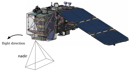
The Copernicus Sentinel-2 mission of the European Space Agency offers free multi-spectral images with a refresh rate of maximum 5 days and a resolution down to 10 m, as detailed in Table 1. Our work focuses on this data source for several reasons. First, multi-spectral information allows to better extract a ship fingerprint and distinguish it from land or man-made structures, as shown in [3,4]. Second, a multi-spectral optical learning based approach can perform detection in both high seas and harbor contexts, while also removing the requirement of storing a vector map of coastlines and performing cloud removal as a pre-processing step. Thus, it could be adapted to a real-time, on-board satellite setting and is not affected by jamming.

Table 1.
Sentinel-2 satellite and capabilities.
Although ship detection is a challenging task, ship identification in remote-sensing images is even more difficult [5]. A coarse identification could be made by ship type (container ship, fishing vessel, barge, cruiseliner, etc.) using supervised classification, with accuracy that should be closely related to image resolution. However, to establish ship identity uniquely, it does not seem feasible with the Sentinel-2 sensor to extract features fit for this purpose, such as measurement of ships to meter precision, extracting exact contours, or detecting salient unique traits of different ships. Our work focuses on detection but the approach is generic and could be extended to other sensors with better resolution, eventually allowing identification.
Recent remote sensing approaches based on machine learning require large amounts of annotated data. Some efforts to collect and annotate data have been made for VHR images, for SAR and for Sentinel 2, but, for the latter, these works did not target ship detection in particular. For object detection using convolutional neural networks (CNN), an interesting way to overcome the lack of data is to use transfer learning. This is achieved either by using CNNs pretrained on large labeled data sets gathered in a sufficiently “close” domain (such as digital photographs), or by pretraining a neural network on the satellite image domain. The latter can be done through an unsupervised pipeline using self-supervised learning (SSL) [6], a contrastive learning paradigm that extracts useful patterns, learns invariances and disentangles causal factors in the training data. Features learned this way are better adapted for transfer learning of few-shot object detectors. We propose to use this paradigm to create a ship detector with few data.
1.1. Related Work and Motivations
For VHR images, a large amount of literature exists, with the number of works following the increasing number of sensors and the quantity of publicly available data [7,8]. Many of these approaches focused on detecting ships with classical image processing pipelines: image processing using spectral indices or histograms (e.g., sea-land segmentation, cloud removal), ship candidate extraction (e.g., threshold, anomaly detection, saliency), and, then, rule-based ship identification or classification using statistical methods. Virtually all of these works focus on VHR images with R,G,B, and PAN bands, occasionally with the addition of NIR, with resolution less than 5 m. Deep learning was applied to images with under 1m resolution by using object detection convolutional neural networks (CNN): R-CNNs [9,10], YOLO [11,12], U-Net [13,14].
For SAR imagery, [1] reviews four operational ship detectors that work on multiple sensors. All of the approaches use classical processing chains and start by filtering out land pixels. This filter is either based on shapefiles or on land/water segmentation masks generated from the SAR image. However, in both cases, a large margin is taken around the coastlines, eliminating any ships that are moored in ports. Deep learning was also applied to SAR ship detection, with notable results detailed in [15].
In multi-spectral images, the most notable work is [4] which uses SVMs to identify water, cloud, and land pixels and then builds a CNN to fuse multiple spectral channels. This fusion network predicts whether objects in the water are ships. Other approaches, such as [3], rely on hand made rules on size and spectral values to distinguish between ships, clouds, islands, and icebergs. The only Sentinel 2 ship dataset publicly available is [16] but it only includes small size image chips and weak annotations for precise localization, i.e., a single point for each ship, obtained by geo-referencing AIS GPS coordinates to pixel coordinates in the chips.
Although large datasets exist for VHR images, for Sentinel-2 none are available with pixel level annotations while usually thousands of examples are needed to train deep learning object detectors. Few-shot learning based approaches can bring interesting perspectives for remote sensing in general and in our setting in particular. Few-shot learning consists in training a neural network with few labeled samples, most often thanks to quality feature extractors upon which transfer learning is performed. One recent method for unsupervised learning of features extractors that enable few-shot learning is contrastive self-supervised learning [6,17]. Contrastive SSL relies on a “pretext training task”, defined by the practitioner, that helps the network to learn invariances and latent patterns in the data [18,19,20].
Several strategies exist for choosing the pretext task: context prediction [21], jigsaw puzzle, or simply by considering various augmented views. The latter is used by [22,23] for remote sensing applications like land use classification and change detection.
1.2. Contributions
In this work, we make two contributions:
- (1)
- A deep learning pipeline for ship detection with few training examples. We take advantage of self-supervised learning to learn features on large non-annotated datasets of Sentinel 2 images and we learn a ship detector using few-shot transfer learning;
- (2)
- A novel Sentinel 2 ship detection dataset, with 16 images of harbours with a total of 1053 ship annotations at the pixel level.
2. Materials and Methods
Our approach is based on a U-Net architecture with a ResNet-50 backbone to produce binary ship/no-ship segmentation masks of the input image. U-Net has been used extensively in remote sensing applications, traditionally with a simple downsampling path of consecutive convolution blocks with no downward skip connections.
2.1. U-Net Architecture
Although the “vanilla” version of U-Net is usually trained from scratch, in this work we modify it to use a different backbone, ResNet-50, that can be easily pre-trained separately using a contrastive objective and then plugged into the U-Net architecture. Figure 1 describes graphically this architecture.

Figure 1.
ResNet50-UNET architecture (s2 = stride 2px). The FC layer of ResNet50 has been removed. Numbers show output channels of each block.
The network takes as input a 64 × 64 pixel patch with 6 channels corresponding to the B2 (B), B3 (G), B4 (R), B8 (NIR), and B11 and B12 (SWIR) spectral channels. The downsampling path reduces the width and height through strided convolution layers while increasing the numbers of channels. The last layer of the ResNet50 backbone has 2048 channels. A “bridge” is added between this layer and the first UPconv block of the upsampling branch of the U-Net.
The output layer uses pointwise convolution, equivalent to applying a fully-connected layer at each pixel, to produce a 2-dimensional vector . This vector contains class probabilities of the pixel belonging to the ship class . The classification decision p is taken by of this output vector in each pixel, giving a binary mask at the resolution of the input image.
The input patch size, 64 × 64 pixels, is chosen such that SSL training of the ResNet-50 backbone is technically possible on a desktop GPU, as detailed in the following section.
2.2. Self-Supervised Learning of ResNet-50 Backbone
We chose the MoCo architecture [24] for the self-supervised pretraining of the ResNet-50 backbone. In this approach, a dictionary of embeddings from previous versions of the feature extractor are cached to provide, without additional computation, a large amount of negative examples to a contrastive loss at each iteration.
The main advantage of MoCo is that it does not require large batch sizes [6] and, thus, can be trained on a single desktop GPU. In this approach, only few embeddings of negatives are computed in each training iteration using the current version of the encoder. Many other embeddings, computed with previous versions of the encoder, are cached and, thus, reused. The encoder is updated using a momentum rule based on the encoder weights, thus converging more slowly towards the encoder.
The Moco algorithm is described in Figure 2. Here and are two 64 × 64 pixel patches. We designate as the query patch and as “negatives”. At each training iteration a new query patch is considered and a “positive” patch is generated by the pretext task. A number of random negative patches are sampled and passed through the momentum encoder to produce “negative” embeddings. The similarity, is computed between the query patch and the embedding of the positive patch and of the negatives. The embeddings of the negatives are the union of those computed from the negatives in the current batch and those taken from a FIFO queue of negative embeddings. We use the NTXent loss on the similarity measure:
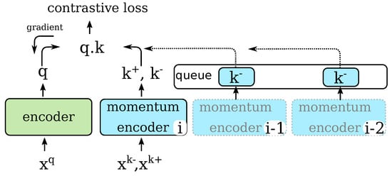
Figure 2.
MoCo training algorithm [6]: negative embeddings from momentum encoders at previous iterations (, , etc.) are cached and reused at iteration i.
The encoder and momentum encoder are both ResNet-50 networks, as described in the backbone block of Figure 1 but with an additional average pooling and fully connected layers on top. The fully connected layer has 512 output neurons and produces the embedding. The encoder’s parameters are updated with SGD while the momentum encoder’s parameters are updated using Equation (2) where is the momentum value:
Patches in SSL are pre-processed by first clipping to the 3rd and 97th percentile computed, for each band, over the pre-training dataset. Then the patches are standardized by subtracting the mean and dividing by the standard deviation computed on a part of the EuroSAT dataset [25].
2.3. Pretext Task Settings
We implemented two pretext tasks in this work:
- Data-Augmentations (A): it consists in choosing data-augmentations according to the invariances our network needs to learn. In our case, it has to identify ships no matter their orientation, size, even if the water is turbulent or if the background is noisy. Therefore, we applied an augmentation function to our query patch, where is one of: color jitter, random rotations, crop and resize with a small scale difference, slight Gaussian noise:
- Region-wise similarity and data augmentations (RA): learns features that increase the similarity between two patches of the same geographical region. This task is illustrated in Figure 3 and can be formalized as , where is the same as above and generates a geographically close patch. Inspired by [26], this strategy aims to help the network to better cluster together similar regions (land, water bodies, etc.). The maximum distance can be varied to control the average overlap of sampled patches. Larger distance induces increased diversity but can generate patches that are too different from each other (ex: water and land when applying to littoral regions). We test two variants: high distance (RA) and low (RA-lo).
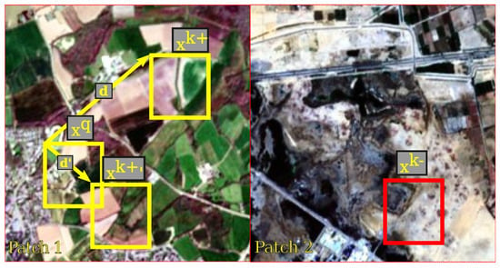 Figure 3. Region based pretext task. Patches and (yellow) constitute a positive pair whereas patches and (red and yellow) form a negative pair.
2.4. U-Net Ship Detector Training
We consider full-size training images and their associated ground truth that is a binary pixel mask for each multi-spectral image. In the mask, pixels with a value of one are ship pixels, and are zeroed otherwise. Next, we sample random 64 × 64 pixel patches from these images, ensuring, however, that at least five pixels of the patch belong to a ship. Since ships are scarce in the images this step re-balances the distribution of ship vs. non-ship pixels in training.
During training we further take into account the class imbalance of pixels by using the focal loss [27] to train the U-Net model. For a prediction and ground truth y:
We set , (corresponding to background pixels) and (corresponding to ship pixels). We train the U-Net detector with the ADAM optimizer while also introducing some data augmentation in training: random vertical and horizontal flips.
We normalize the training patches in the same way as in the pretext task (see Section 2.3).
2.5. Inference
To detect ships with our model we first cut the target image into patches of the same size as in training-64 × 64 pixels-using a regular grid. However, for inference we take these patches with an overlap of 32 pixels. It is well known that U-Net architectures, and CNNs in general have lower performance on the borders of the image than in the center, due to the influence of padding in the backbone. Since our backbone is trained with a contrastive objective task during SSL, this type of padding was the most straightforward approach. When transferred to the U-Net setting, 0-padding introduces artifacts on image borders. We chose to simply cut out 16 pixel wide borders of the patches.
Finally, the full image binary mask is produced by stitching the individual patch masks together. We apply the connected components algorithm with 4-connectivity to extract blobs in this mask. Each blob is considered as a detected ship, without additional filtering.
2.5.1. Filtering Stage
Optionally, we can filter these detections with a water/land mask generated from OpenStreetMap coastline vector data. When enabled, we perform filtering by multiplying the image binary prediction mask with the water mask, before extracting connected components. In this way, ships that are moored will be detected without spillover to peers or land masses. A variation of this filtering involves a water mask than removes littoral regions (in a 600 m range), in order to perform detection only in open sea. This second open-sea mask is obtained by thresholding a distance-transform of the water/land mask. Our pipeline, thus, has an optional filtering stage with two variations: coastline (CO) or open-sea (OS).
2.6. Ship Detection Dataset: S2-SHIPS
To the best of our knowledge, no ship detection Sentinel-2 datasets for both moving and static ships with pixel level annotations has yet to be published. We introduce a novel ship detection dataset made up of littoral and harbor regions images.
This dataset includes 16 L2A images of coastline, ports, and the Suez canal. Figure 4 shows the geographical distribution of the data. The images are of size 1783 × 938, cover 167 sq. km each, and are annotated at the pixel level with a total of 1053 distinct ships. We also provide earth/water masks for these images, rasterized from OpenStreetMap layers.

Figure 4.
S2-SHIPS geographical distribution of image tiles. Points on Western Europe map (middle) represent image tiles in data set for ports of: Southampton, Portsmouth, Brest, Rotterdam (3 tiles), Toulon, Rome, Marseilles.
The ships are from various size, with areas ranging from 100 m (e.g., pleasure boats, small fishing ships) to more than 5000 m (e.g., cargo ships). Since the Sentinel 2 mission does not provide high sea tiles, the images are taken near coasts and we annotated moored ships and ships at sea separately. Our dataset also provides images taken under different weather conditions, including turbulent seas, clouds, or sun glint. Thus, the complex environment surrounding ships in our dataset makes it challenging for ship detection. Several samples are shown in Figure 5.

Figure 5.
S2-SHIPS dataset patch samples: Brest (FR), Toulon (FR), Rotterdam (NL), Colon (PA), Suez Canal (EG). Note that some images have partial cloud cover or rough sea conditions.
We rasterize OpenStreetMap water layers (ocean, major rivers, canals) on the 16 geo-referenced images to produce binary masks of water. These layers sometimes have the contours of peers, jetties, but the annotation of these entities as land is not insured.
2.7. Backbone Pre-Training Datasets
For backbone pre-training with SSL, we look at existing large scale Sentinel 2 datasets. Several have been published in recent years and usually focus on land cover classification or segmentation. Since we do not use labels for pre-training we can use these types of data easily and in large quantities. Some well-known datasets are:
- EuroSAT [25], which is a 10 class land-cover classification dataset containing 27,000 multi-spectral patches of size 64 × 64 pixels. We apply the (A)ugmentation pretext task on this dataset;
- BigEarthNet [28], which is a very large scale multi-label land-cover classification dataset. It contains 590,326 multi-spectral image patches of size 120 × 120 pixels. We randomly crop 320,000 64 × 64 pixel patches from the original dataset and we apply the (A)ugmentation pretext task for BigEarthNet;
- SEN12MS [29], which is a very large curated land cover segmentation dataset, made of Sentinel 1, 2 and MODIS images. It contains 180,662 Sentinel 2 multi-spectral patches of size 256 × 256. For this dataset, we apply both the (A)ugmentation and the region-wise and augmentation (RA) pretext task. For the first one we sample 1,337,360 patches 64 × 64 patches from the 256 × 256 patches in the dataset. For the (RA) and (RA-lo) tasks we sample patches and of size 64 × 64 pixels randomly from the same 256 × 256 patch. The distance between these two “positive” patches can thus be at most 1.2 km for (RA) and 640 m for (RA-lo), while sometimes there can be an overlap.
2.8. Experimental Settings and Parameters
We run the pre-training SSL pipeline for 100 epochs with a learning rate of 0.001 and a cosine annealing schedule. For the augmentation (A) task, we used a batch size of 500 for the EuroSAT and BigEarthNet pretraining and a batch size of 900 for SEN12MS. We trained the pretext task on one GPU with 12 Go of memory for the EuroSAT and BigEarthNet datasets, and on a multi-gpu machine for SEN12MS dataset to accelerate the learning process. The region based pretext (RA) task was applied to SEN12MS using the same hyperparameters as for (A), with a batch size of 500.
Next, we copied the parameters of the ResNet-50 backbone trained with SSL into the corresponding layers of the U-Net. We train the network in two ways: fine-tuning (FT) and transfer learning (TL). The first one, FT, corresponds to training all the layers of the U-NET on the ship detection task, while for the latter, TL, we froze the layers of the backbone.
For the ship detection task, both in the TL and FT modes, we train the network with 100 epochs, with a batch size of 20 and a learning rate of 0.001.
We evaluate our method as a one class object detection algorithm, using the pycocotools package. We focused on object-wise precision, recall and F1-score (harmonic mean of precision and recall) metrics. We also compute the recall for each ship size (a ship is considered as small if its area is under 2500 m², otherwise it is considered as being large), and for each ship location (moored ships or sailing ships).
2.9. Baselines
- ImageNet transfer learning: Instead of pre-training the backbone with SSL, this baseline uses a ResNet-50 encoder pretrained on ImageNet as implemented by the torchvision package. Since these encoders are trained on RGB images, we copy the weights of the first 3 channels of the first layer in order to initialize the channels corresponding to spectral bands B8, B11, and B12. Both the TL and FT ship detector training approach can be applied to this baseline;
- Random initialization: Instead of using a trained backbone network, we initialize the ResNet-50 encoder randomly following the standard Kaiming initialization. Only the fine-tuning (FT) detector training mode is applied when initializing the weights randomly;
- BL-NDWI—Water segmentation baseline with NDWI: We develop a simple baseline which is based on classical image processing techniques. We use the NDWI spectral index and we threshold its value to segment water and non-water pixels. The threshold for the NDWI segmentation is chosen to obtain the best performance on the whole dataset, which may lead to suboptimal choices for some images.Next, we eliminate land pixels using the water/land segmentation (CO) (Section 2.5.1) map, giving a ship proposal map. We consider non-water pixels in what are normally water regions to potentially be ships. We extract connected components and we eliminate those that have a width and height greater than 50 pixels (500 m) since no ships larger than this size exist. These are due to islands or sandbanks not correctly mapped in OpenStreetMap layers or thin water banks where the coastline annotation in OpenStreetMap is imprecise.Finally, we do several filtering passes on the resulting proposal map: morphological opening and we apply watershed segmentation on the resulting map to identify individual ships.
3. Results
Our evaluation has three objectives: (1) study the impact of the SSL pre-training strategy of the backbone on the final performance of the ship detector, (2) compare our SSL-trained U-Net to the baselines and, (3) analyze the few-shot performance of SSL.
3.1. Self-Supervised Learning Approach Analysis
We train the ship detector on the S2-SHIPS dataset in the leave-one-out setting: out of N images we choose for training and one for testing. For certain geographical regions there are several images in the dataset while for others only one. Therefore, by varying the testing and training images we measure the transferability of the learned detector, for different levels of domain difference between training and testing sets. We do not perform cross-validation, the hyperparameters for U-Net are chosen a priori and not optimized.
We obtain 16 folds with 15 training images and one testing image. The training set consists of patches that match the ship presence criterion described in Section 2.4, extracted from the original images. This sampling produced about 1800 patches on average per fold. We report precision, recall, and F1-score averaged over the 16 folds, averaged over 5 runs of the experiments. We do not report standard deviations as they were always insignificant.
Our initial aim is to evaluate the overall performance of the detector, irrespective of land cover in the images. Thus, we first test without the filtering stage, and the precision results reflect false positives both on land and at sea.
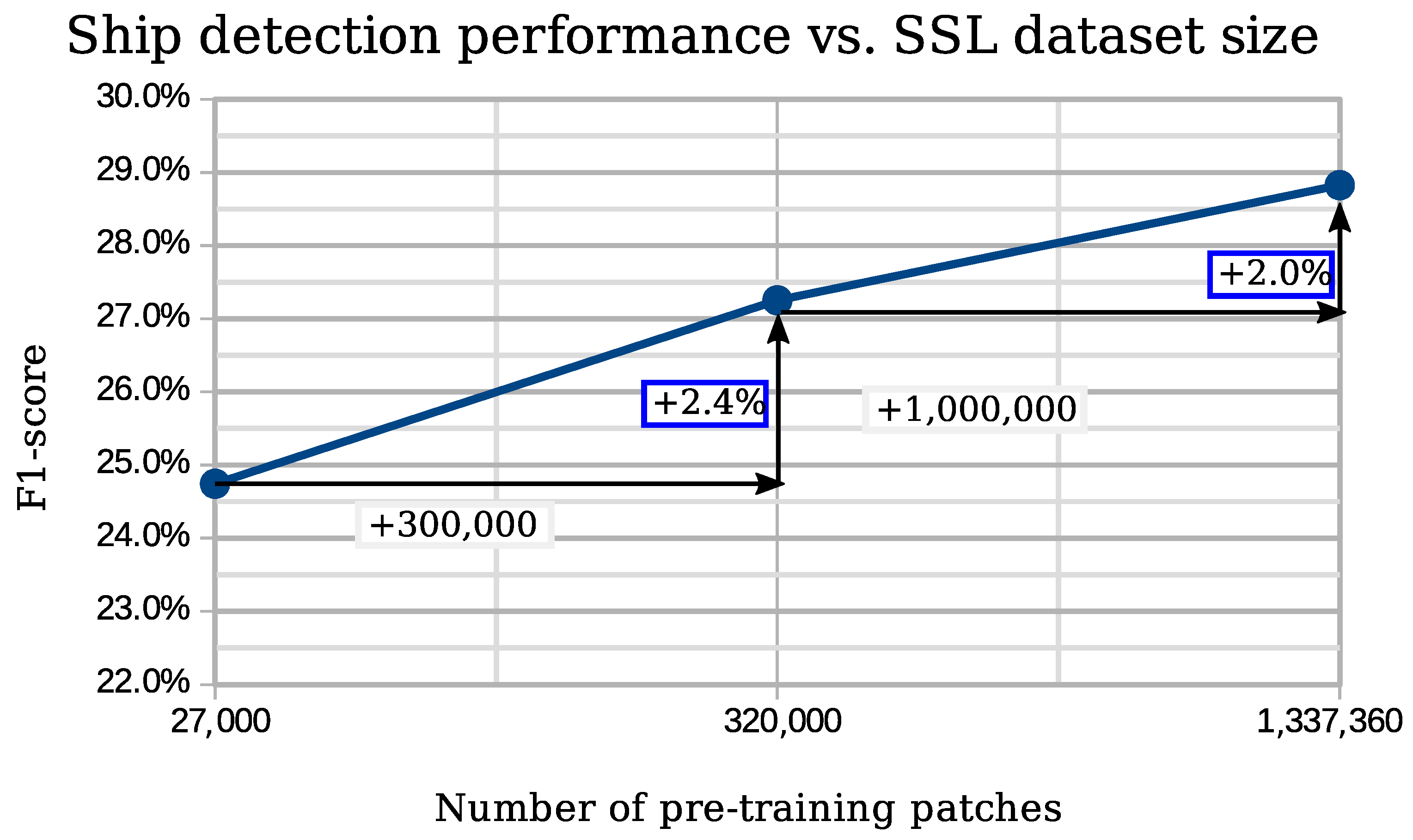
Table 2 presents the results of this comparison. First, we can observe that there is a strong relationship between the dataset size and the performance attained. To see this in more detail, in Figure 6 we show graphically the difference in F1 score depending on the size of the pre-training dataset, under the (A)ugmentation pre-text task, using transfer learning (TL).

Table 2.
Average performance measures for the various SSL settings, over 5 runs over the 16 folds of the S2-SHIPS dataset. Best results are presented in bold font. Note that the F1-score here is the average of F1 scores over folds.
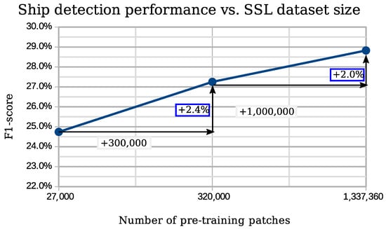
Figure 6.
Impact of dataset size on F1 score in the TL settings with the A pretext task.
Using the large SEN12MS dataset we obtain four percentage points of F1 score more than with EuroSAT for the same pretext task. In Table 2, we note that this gain in performance is due to a stronger gain of relative precision than the loss of relative recall.
Table 2 also shows that the region-wise similarity, coupled to augmentation (RA), outperforms augmentation-only pre-training (four F1 percentage points in the FT setting). Furthermore, a large maximum positive patch distance is beneficial, compared to low-distance/high overlap (RA-lo).
Additionally, Table 3 shows how the false alarm rate drastically decreases from 1.70 ship/km² for EuroSAT to 1.20 ship/km² for SEN12MS-A without filtering, and down to 0.14 ships/km² for the open-sea setting (OS).

Table 3.
False alarm rates for the various SSL settings (Transfer Learning). Best results are presented in bold font.
3.2. Comparison of SSL to Baseline Approaches
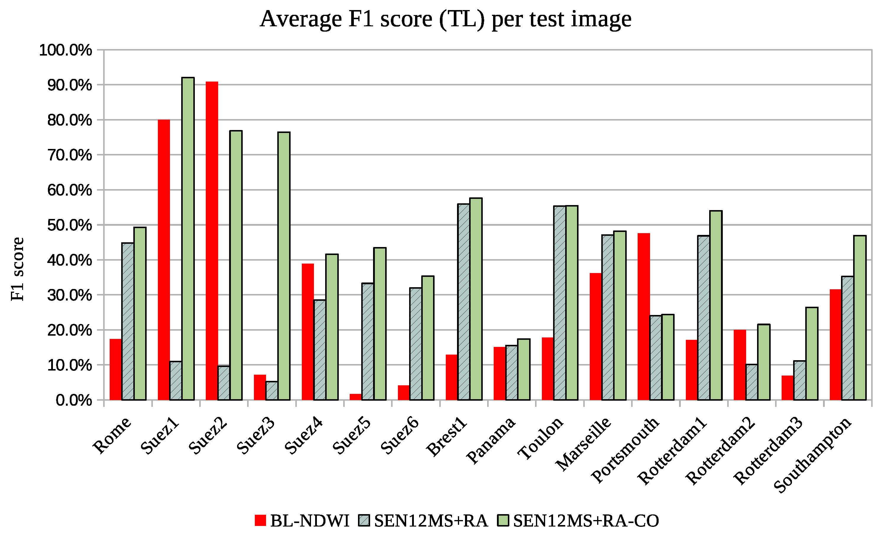
Next, we compare our best pre-training method (SEN12MS+RA) to the ImageNet pretraining and to the BL-NDWI baseline. Table 4 presents this comparison, Table 5 analyzes the false alarm rate for the different methods and Figure 7 compares the results by image.

Table 4.
Ship detection performance—best SSL based approach versus baselines. Average precision, recall, and F1-score computed over the 16 folds. Best results are presented in bold font.

Table 5.
Average false alarm rate comparison of the best SSL result versus the baselines. Best results are presented in bold font.
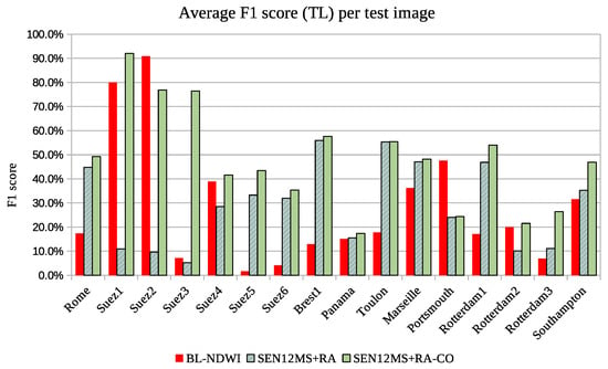
Figure 7.
F1-score variation on all S2-SHIPS dataset for NDWI, SEN12MS-RA (no filt.) and SEN12MS-RA with CO filt.
Table 4 shows that when all methods are filtered with land/sea map, deep learning algorithms lead to largely better results than the BL-NDWI method: in transfer learning mode, it gains 20 percentage points of F1 and double the recall. This means that many ships are not detected with BL-NDWI, and one explanation could be the threshold choice for the NDWI that is not generally optimal to all images. The problem of sub-optimal threshold can be seen in Figure 7, where, for some test images, such as Suez 1 and 2, the threshold is almost perfectly chosen, whereas on Suez 3, Suez 5, and Suez 6 the detection is really weak. As the threshold of the NDWI is chosen to maximize performance over the whole dataset, it is suboptimal on individual images.
For deep learning methods, such as SEN12MS-RA, generalizing problems are evidenced on images Suez 2, Panama, and Rotterdam 2, but this is mainly due to the challenging conditions induced by those test images, rather than domain difference: large land cover (Suez canal), clouds (Rotterdam, Panama), and turbulent sea (Panama).
Our SSL based pipeline achieves similar results to ImageNet pre-training in the transfer learning setting and two percentage points higher F1 score in the fine-tuning setting. It is worth noticing that training from scratch achieved better F1 score in the fine-tuning setting. When training on 15 images, learning from scratch seems a better choice due to simplicity and better performance. Indeed, most works use this setting for remote sensing applications. However, our aim is to study few shot learning performance and in this setting, as shown in the following sections, learning from scratch is disadvantaged.
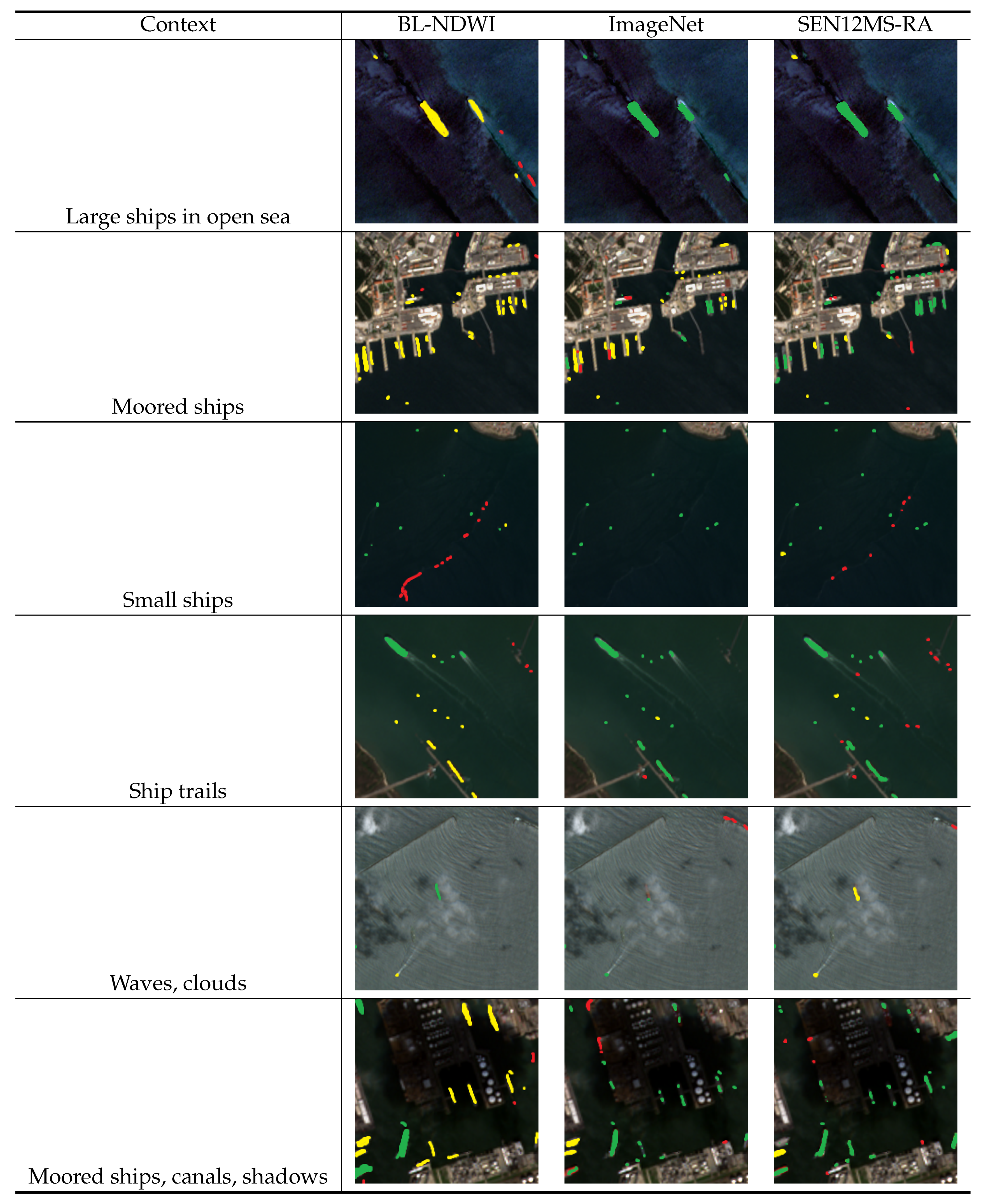
Generally, deep learning methods are weak in areas with dark background (grass, cloud shadow), waves or large boat trail, where they lead to many false positives. Figure 8 presents a qualitative analysis of their results. In these conditions, networks trained from scratch or pretrained on EuroSAT and BigEarthNet lead to the worst results. Some piers and docks are also confused with ships. Deep learning methods seem to be robust to brightness, water color, or environment difference, and they also rarely predict small islands as ships.
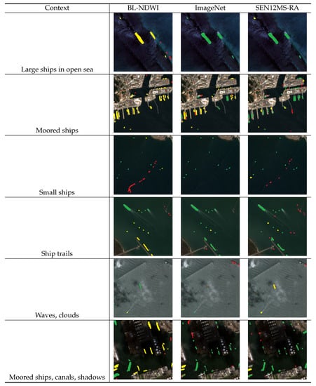
Figure 8.
Ship detection samples, in various conditions. In green are drawn true positives, in red false positives and in yellow missed ships (false negatives). Best viewed in color.
3.3. Few-Shot Performance of the Methods under Study
To evaluate the performance dynamics of the proposed method in the few-shot learning setting we split the dataset into two parts. The training set contains 13 images and the test set three: one from the Suez canal, a second from Brest and the last one from Rotterdam. We vary the number of training images from 1 to 13, which corresponds to a variation in the number of distinct ships from 42 to 742. This experiment aims to highlight the network’s robustness towards training dataset size and diversity (sun glint, water color, etc.).
Varying the number of training samples shows that SSL methods trained on large datasets, especially with the region based pretext task, achieve competitive and even better results than ImageNet pretrained networks fine-tuned on a small amount of data. Indeed, in Figure 9, we see that having only between 200 and 300 training examples is sufficient for SEN12MS-RA method to get close to a F1 score of 35%, while ImageNet network needs at least 350 samples to reach this performance. This experiment also confirms the importance of the pretext task: the region invariances induced by SEN12MS-RA method increased considerably the performances. Indeed, only 290 ships are needed by SEN12MS-RA to get 92% of the best performances obtained with 750 training ships, while other methods need at least a third more training ships.
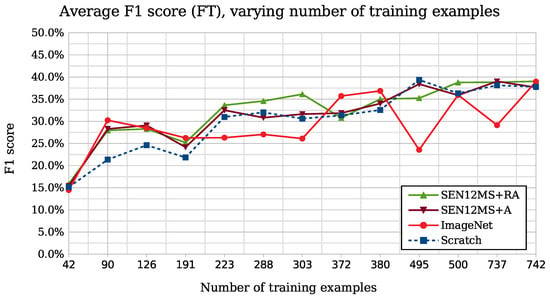
Figure 9.
Impact of the number of training ships variation on mean F1 score calculated on Brest, Rotterdam, and Suez canal.
Moreover, in a few-shot setting, with 126 training examples, Figure 10 analyzes the performance of the methods under study on different sub-classifications of the ships: small vs large and moored or at sea. SEN12MS-A and SEN12MS-RA have a better recall than ImageNet or training from scratch by far. SEN12MS pretraining is significantly better at detecting moored ships than other methods, including ImageNet.
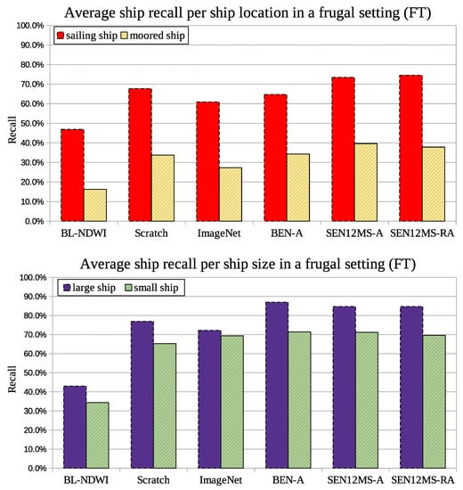
Figure 10.
Ship detection performance according on ship size and location, with a frugal setting (126 training ships).
The weakness of ImageNet may come from the fact that it needs to fine-tune its weights further, because of the large domain difference that exists when transferring the knowledge learned on object-centric datasets to remote sensing images. Therefore, robust SSL methods give a good boost when having few training samples, unlike networks trained from scratch or pretrained on ImageNet.
4. Discussion
Globally, the results allow us to conclude that deep learning techniques achieve promising results. In all cases (close to shore and open-sea) recall is high, more than 75%. We obtained less than 0.14 false alerts per square kilometer in the open sea and close to the sea shore, the false alarm rate is around 1 ship/km. Although the BL-NDWI baseline could be improved by finding more optimal NDWI thresholds for each image, the performance difference with respect to deep learning approaches seems hard to make up for.
Networks trained with SSL achieve better results compared with ImageNet pretrained ones. In the few-shot setting, SSL pre-training is usually better and more stable. When sufficient examples are available SSL pretraining is as good as ImageNet or training from scratch. We notice also that performance increases with the size of the pre-training datasets. Since these are not annotated it is easy to build such datasets. The ones chosen here have no relation to the ship detection problem at hand, thus no significant effort is needed to select the images in these datasets.
The pretext task needs to be chosen according to the downstream task in order to learn the needed invariances. The region based pretext task looks promising probably because it helps the encoder to better cluster together similar elements, such as water, agriculture crops, or residential areas, while a simple pretext task data-augmentation only focuses on color or noise invariances. The benefit of such pretext task can be seen in our case as it lowers the number of false positives over land and near the shore.
In terms of computational complexity, the difference between all deep learning methods lies in the way we pre-train the weights. Compared to the supervised pipelines that can be used to train a ResNet-50 on ImageNet dataset, the self-supervised pipeline has a similar complexity but requires much larger batch size. This is particularly problematic for multi-spectral images, and a GPU with at least 8 Go of memory is necessary. The pretext task training is time-consuming: it took us nearly two days to train it on SEN12MS dataset using a multi-GPU machine (4 GPU with a total of 64 Go of memory). Training on a single desktop GPU with at least 8 Go of memory is feasible, but lasts longer.
5. Conclusions
We presented a method to train a ship detector in Sentinel-2 images using self-supervised learning. Our method plugs in a SSL-trained backbone in a U-NET architecture. It achieved better or similar results to standard deep-learning approaches and significantly better results than a spectral index based method. The choice of pretext task in the SSL stage is a major source of performance improvements.
Further studies should focus on the design of a more effective pretext task. Our work shows that there is room for improvement although the direction towards this goal remains unclear. Instead of hand-designed pretext tasks, learning a better pretext task could be a fruitful avenue of research. However, the computational cost of pre-training is high, so it would be necessary to first reduce this cost or to approximate the pre-training stage performance with a light-weight proxy model.
The SSL pipeline can be applied to networks where no ImageNet pretraining is available, such as custom architectures specific to remote sensing. Thus, an interesting research goal would be training, through SSL, a feature extractor designed for remote-sensing applications, that improves upon learning from scratch or ImageNet pretraining by a large margin.
For ship detection, our image-based approach is still two orders of magnitude away from the false alert performance of methods applied on SAR images [1]. To improve image-based ship detection, a better network backbone could be studied, more adapted to small objects. Furthermore, it would be better to include cloud filtering and land/water classification explicitly in the network. Although adding more data is always a good idea, the few-shot setting is more challenging and can bring about more methodological improvements in deep learning for remote sensing.
Author Contributions
Software, validation, data curation, A.C.; supervision, A.S.; methodology, writing: A.C. and A.S. All authors have read and agreed to the published version of the manuscript.
Funding
This project has received funding from the European Union’s Horizon 2020 research and innovation programme under grant agreement No 101016798. This document reflects only the author’s view and the European Commission is not responsible for any use that may be made of the information it contains.

Data Availability Statement
github.com/alina2204/contrastive_SSL_ship_detection (accessed on 10 September 2021).
Conflicts of Interest
The authors declare no conflict of interest.
References
- Stasolla, M.; Mallorqui, J.J.; Margarit, G.; Santamaria, C.; Walker, N. A Comparative Study of Operational Vessel Detectors for Maritime Surveillance Using Satellite-Borne Synthetic Aperture Radar. IEEE J. Sel. Top. Appl. Earth Obs. Remote Sens. 2016, 9, 2687–2701. [Google Scholar] [CrossRef] [Green Version]
- Yang, K.; Ye, W.; Ma, F.; Li, G.; Tong, Q. A Large-Scene Deceptive Jamming Method for Space-Borne SAR Based on Time-Delay and Frequency-Shift with Template Segmentation. Remote Sens. 2020, 12, 53. [Google Scholar] [CrossRef] [Green Version]
- Heiselberg, P.; Heiselberg, H. Ship-Iceberg discrimination in Sentinel-2 multispectral imagery by supervised classification. Remote Sens. 2017, 9, 1156. [Google Scholar] [CrossRef] [Green Version]
- Xie, X.; Li, B.; Wei, X. Ship Detection in Multispectral Satellite Images Under Complex Environment. Remote Sens. 2020, 12, 792. [Google Scholar] [CrossRef] [Green Version]
- Heiselberg, H. A Direct and Fast Methodology for Ship Recognition in Sentinel-2 Multispectral Imagery. Remote Sens. 2016, 8, 1033. [Google Scholar] [CrossRef] [Green Version]
- Jaiswal, A.; Babu, A.R.; Zadeh, M.Z.; Banerjee, D.; Makedon, F. A survey on contrastive self-supervised learning. Technologies 2021, 9, 2. [Google Scholar] [CrossRef]
- Kanjir, U.; Greidanus, H.; Oštir, K. Vessel detection and classification from spaceborne optical images: A literature survey. Remote Sens. Environ. 2018, 207, 1–26. [Google Scholar] [CrossRef]
- Li, B.; Xie, X.; Wei, X.; Tang, W. Ship detection and classification from optical remote sensing images: A survey. Chin. J. Aeronaut. 2020, 34, 145–163. [Google Scholar] [CrossRef]
- Zhang, S.; Wu, R.; Xu, K.; Wang, J.; Sun, W. R-CNN-Based Ship Detection from High Resolution Remote Sensing Imagery. Remote Sens. 2019, 11, 631. [Google Scholar] [CrossRef] [Green Version]
- Liu, Z.; Yuan, L.; Weng, L.; Yang, Y. A high resolution optical satellite image dataset for ship recognition and some new baselines. In Proceedings of the International Conference on Pattern Recognition Applications and Methods, Porto, Portugal, 24–26 February 2017; Volume 2, pp. 324–331. [Google Scholar]
- Redmon, J.; Divvala, S.; Girshick, R.; Farhadi, A. You only look once: Unified, real-time object detection. In Proceedings of the IEEE Conference on Computer Vision and Pattern Recognition, Las Vegas, NV, USA, 27–30 June 2016; pp. 779–788. [Google Scholar]
- Tang, G.; Liu, S.; Fujino, I.; Claramunt, C.; Wang, Y.; Men, S. H-YOLO: A Single-Shot Ship Detection Approach Based on Region of Interest Preselected Network. Remote Sens. 2020, 12, 4192. [Google Scholar] [CrossRef]
- Ronneberger, O.; Fischer, P.; Brox, T. U-net: Convolutional networks for biomedical image segmentation. In Proceedings of the International Conference on Medical Image Computing and Computer-Assisted Intervention, Munich, Germany, 5–9 October 2015; pp. 234–241. [Google Scholar]
- Karki, S.; Kulkarni, S. Ship Detection and Segmentation using Unet. In Proceedings of the 2021 International Conference on Advances in Electrical, Computing, Communication and Sustainable Technologies (ICAECT), Bhilai, India, 19–20 February 2021; pp. 1–7. [Google Scholar]
- Tang, G.; Zhuge, Y.; Claramunt, C.; Men, S. N-YOLO: A SAR Ship Detection Using Noise-Classifying and Complete-Target Extraction. Remote Sens. 2021, 13, 871. [Google Scholar] [CrossRef]
- Lagrange, A.; De Vieilleville, F.; Ruiloba, R.; Le Saux, B.; Mathieu, P.P. CORTEX: Open training datasets of Sentinel images: Ships (Sentinel-2) and refugee camps detection (Sentinel-1 and 2). In Proceedings of the ESA EO PHI-WEEK 2020, Virtual Event, 28 September–2 October 2020. [Google Scholar] [CrossRef]
- Liu, X.; Zhang, F.; Hou, Z.; Mian, L.; Wang, Z.; Zhang, J.; Tang, J. Self-supervised learning: Generative or contrastive. IEEE Trans. Knowl. Data Eng. 2021. [Google Scholar] [CrossRef]
- Purushwalkam, S.; Gupta, A. Demystifying contrastive self-supervised learning: Invariances, augmentations and dataset biases. arXiv 2020, arXiv:2007.13916. [Google Scholar]
- Zimmermann, R.S.; Sharma, Y.; Schneider, S.; Bethge, M.; Brendel, W. Contrastive Learning Inverts the Data Generating Process. arXiv 2021, arXiv:2102.08850. [Google Scholar]
- Tsai, Y.H.H.; Wu, Y.; Salakhutdinov, R.; Morency, L.P. Self-supervised learning from a multi-view perspective. arXiv 2020, arXiv:2006.05576. [Google Scholar]
- Doersch, C.; Gupta, A.; Efros, A.A. Unsupervised visual representation learning by context prediction. In Proceedings of the IEEE International Conference on Computer Vision, Santiago, Chile, 7–13 December 2015; pp. 1422–1430. [Google Scholar]
- Tao, C.; Qi, J.; Lu, W.; Wang, H.; Li, H. Remote sensing image scene classification with self-supervised paradigm under limited labeled samples. IEEE Geosci. Remote Sens. Lett. 2020. [Google Scholar] [CrossRef]
- Leenstra, M.; Marcos, D.; Bovolo, F.; Tuia, D. Self-supervised pre-training enhances change detection in Sentinel-2 imagery. arXiv 2021, arXiv:2101.08122. [Google Scholar]
- He, K.; Fan, H.; Wu, Y.; Xie, S.; Girshick, R. Momentum contrast for unsupervised visual representation learning. In Proceedings of the IEEE/CVF Conference on Computer Vision and Pattern Recognition, Seattle, WA, USA, 14–19 June 2020; pp. 9729–9738. [Google Scholar]
- Helber, P.; Bischke, B.; Dengel, A.; Borth, D. Eurosat: A novel dataset and deep learning benchmark for land use and land cover classification. IEEE J. Sel. Top. Appl. Earth Obs. Remote Sens. 2019, 12, 2217–2226. [Google Scholar] [CrossRef] [Green Version]
- Jung, H.; Oh, Y.; Jeong, S.; Lee, C.; Jeon, T. Contrastive Self-Supervised Learning With Smoothed Representation for Remote Sensing. IEEE Geosci. Remote Sens. Lett. 2021. [Google Scholar] [CrossRef]
- Lin, T.Y.; Goyal, P.; Girshick, R.; He, K.; Dollár, P. Focal Loss for Dense Object Detection. In Proceedings of the 2017 IEEE International Conference on Computer Vision (ICCV), Venice, Italy, 22–29 October 2017; pp. 2999–3007. [Google Scholar] [CrossRef] [Green Version]
- Sumbul, G.; Kang, J.; Kreuziger, T.; Marcelino, F.; Costa, H.; Benevides, P.; Caetano, M.; Demir, B. BigEarthNet dataset with a new class-nomenclature for remote sensing image understanding. arXiv 2020, arXiv:2001.06372. [Google Scholar]
- Schmitt, M.; Hughes, L.H.; Qiu, C.; Zhu, X.X. SEN12MS—A Curated Dataset of Georeferenced Multi-Spectral Sentinel-1/2 Imagery for Deep Learning and Data Fusion. arXiv 2019, arXiv:1906.07789. [Google Scholar] [CrossRef] [Green Version]
Publisher’s Note: MDPI stays neutral with regard to jurisdictional claims in published maps and institutional affiliations. |
© 2021 by the authors. Licensee MDPI, Basel, Switzerland. This article is an open access article distributed under the terms and conditions of the Creative Commons Attribution (CC BY) license (https://creativecommons.org/licenses/by/4.0/).


