Abstract
The Surface Urban Heat Islands (SUHI) phenomenon has adverse environmental consequences on human activities, biophysical and ecological systems. In this study, Land Surface Temperature (LST) from Landsat and Sentinel-2 satellites is used to investigate the contribution of potential factors that generate the SUHI phenomenon. We employ Principal Component Analysis (PCA) and Multiple Linear Regression (MLR) techniques to model the main temporal and spatial SUHI patterns of Cartago, Colombia, for the period 2001–2020. We test and evaluate the performance of three different emissivity models to retrieve LST. The fractional vegetation cover model using Sentinel-2 data provides the best results with R2 = 0.78, while the ASTER Global Emissivity Dataset v3 and the land surface emissivity model provide R2 = 0.27 and R2 = 0.26, respectively. Our SUHI model reveals that the factors with the highest impact are the Normalized Difference Water Index (NDWI) and the Normalized Difference Build-up Index (NDBI). Furthermore, we incorporate a weighted Naïve Bayes Machine Learning (NBML) algorithm to identify areas prone to extreme temperatures that can be used to define and apply normative actions to mitigate the negative consequences of SUHI. Our NBML approach demonstrates the suitability of the new SUHI model with uncertainty within 95%, against the 88% given by the Support Vector Machine (SVM) approach.
1. Introduction
Urban expansion transforms natural areas into surfaces covered with concrete, asphalt, and buildings (highly impervious materials), reducing evapotranspiration and decreasing the cooling capacity of the air, which in turn helps to reduce the impacts of high urban surface temperature on the urban surface. Due to the existing urban growth, the climate in these areas becomes warmer than the regional areas of the suburban and rural regions, resulting in the phenomenon of Urban Heat Islands (UHI) [1]. The UHI refers to a phenomenon in which urban areas tend to have higher air or surface temperatures than their surroundings [2]. Traditionally, terrestrial observation methods, such as ground meteorological stations that record specific values of air temperature, have been used to model UHI [3]. The difference between air temperature measurements recovered from urban and rural meteorological stations is a direct method used to model UHI [4]. However, the high heterogeneity in urban areas makes temperature spatially diverse, making it difficult for a small number of stations to realistically represent the real variability [5]. When the UHI phenomenon is monitored by remote sensing, it is referred to as Surface Urban Heat Island (SUHI). The reason is that the parameter considered here is the Land Surface Temperature (LST), which differs from studies of air temperature [6]. Therefore, LST is an essential variable to characterize SUHI, which has been listed as an essential climate variable of the World Meteorological Organization program. This variable is an important indicator of the energy balance between the atmosphere and the surface of the Earth [7]. Zhou et al. [8] presented a broad review of the SUHI phenomenon and suggested several methods of analysis through the integration of remote sensing data, thermal trends, field observations, and numerical modeling. Sekerteking and Zadbagher [9] suggest that to model and simulate LST, it would be important to investigate the performance of various Machine Learning methods associated with statistical and numerical models. Li et al. [10] and Mei et al. [11] pointed out that one of the problems to be solved in inference models of LST or geographic variables is to evaluate the influence of contributing factors.
Land-use land-cover changes (LULC) and spectral indices from satellite data, such as, e.g., Normalized Difference Vegetation Index (NDVI) or Normalized Difference Water Index (NDWI), have been used extensively to investigate the relationships between urban and biophysical systems, as well as their impact on surface temperature [12,13,14,15]. LULCs are due to complex interactions between the urban system and the biophysical environment that produce significant changes in local temperatures. In a recent work published by Shi et al. [16], eight parameters were referred to as urban design factors, where thermal properties of building materials, vegetation, vegetation cover ratio, and ground emissivity were taken into account. The authors suggested the need to detect more potential factors affecting this phenomenon.
Understanding and quantifying urban temperatures in space and time are significantly relevant for city planners in defining policies that generate adaptation strategies to mitigate the SUHI effects. A very useful tool is Principal Component Analysis (PCA), a multivariate statistical technique that aims to preserve the total variance and reduce the dimensionality of the data set, while eliminating redundancy in the data [17]. Several authors have used this technique to detect spatial patterns of biophysical factors by synthesizing information from a set of images [18,19,20]. Multiple Linear Regression (MLR) analysis is an approach used to evaluate the relationship between independent and dependent factors [21]. This method has also been widely used to determine the relationship of various environmental factors [22,23,24].
Advanced nonlinear analysis techniques, such as Machine Learning, have been applied in numerous studies that require analyzing variables related to urban thermal changes. Some examples are population density, land cover, and urbanization [25,26,27,28,29]. Voelkel and Shandas [30] implemented a UHI model to detect a daily distribution of temperatures. Their results revealed that a random forest (RF) model performed better in predicting temperature. Furthermore, Zumwald et al. [31] developed a model to create high-resolution air temperature maps. This model makes predictions by integrating an RF algorithm with low-cost weather stations. It is important to note that the behavior of SUHI varies over time and is associated with factors such as human development and changes in land use. In this sense, Kafy et al. [32] formulated a seasonal thermal prediction influenced by LULC through Cellular Automata and Artificial Neural Network algorithms. Their findings indicated that by 2039, the urban growth of Cumilla, and Bangladesh, plus the decrease in land cover, will cause 30% of cities to experience temperatures above 33 °C. Shi et al. [33] noted that the use of time series and Machine Learning techniques is a growing trend in SUHI research.
Several studies have widely documented the influence of spectral indices such as the NDBI, NDVI and Normalized Difference Water Index (NDWI) on the SUHI phenomenon [34,35]. However, none of these authors considered the weighted contribution of the factors to temperature changes, while it is an interesting analysis that can identify which factors generate the greatest influence on SUHI. On the basis of these factors, specific adaptation measures to thermal change can be defined and applied. The main novelty of the approach proposed in this work is the application of a weighted Naïve Bayes Machine Learning (NBML) algorithm to segment the geographical space into regions of different thermal intensity, not explored in previous literature.
Understanding and quantifying urban temperatures in space and time is significantly relevant for city planners in defining policies that generate adaptation strategies in the face of adverse effects of SUHI. Here we study the application and assessment of modeling procedures that allow evaluating the contribution of various factors to SUHI. For this purpose, a combination of PCA and MLR techniques applied along with Machine Learning Algorithms is used to detect high thermal intensity patterns in the tropical Colombian Andean city of Cartago. Although SUHI is a derived quantity, expressed as the difference between urban and rural LST, the delimitation of thermal zones using LST ranges allows establishing comparisons with other zones, e.g., rural areas, and classifies the space into zones with greater or lesser thermal activity. In this study, the LST ranges are taken from Wang et al. [36], as they are based on statistical criteria, and they appear to conveniently reflect the LST differences of urban areas with their surroundings. The spatial patterns of the SUHI phenomenon can be represented through LST ranges, which, combined with the weights of the involved variables, are further classified using Machine Learning algorithms.
The methodology suggested in this article establishes an effective method for assessing SUHI patterns, locally, and attempts to draw several recommendations for planning sustainable urban development and for the regeneration of areas with thermal excesses.
2. Materials and Methods
2.1. Study Area
The city of Cartago is located in the south-west area of Colombia in the Andean region at an altitude of 917 m above sea level. It has an extension of 279 km2 with moderate topographic relief. The geodetic coordinates of the city center are 4.75° N and 75.9° W. This area belongs to Valle del Cauca Department and is surrounded by the Cauca and La Vieja rivers.
The climate in this area is tropical dry and the average air temperature is 23.8 °C, with an annual rainfall of 1578 mm. March is the warmest month with an average temperature of 24.3 °C, while October is the coldest with 23.3 °C. According to official reports, the urban population growth rate during 2001–2020 was 12.3%, while the rural population decreased by 44% [37]. The population density is 464 inhabitants per km2. The appearance of new urban units (red oval areas in Figure 1) denotes the urban growth from the city center to the north-east, near the La Vieja River, as well as to the south-east and south-west. Temperatures in tropical zones show small changes throughout the year. According to official reports from the study area, the difference between the average temperature of the warmest month and that of the coldest month is 1 °C [38].
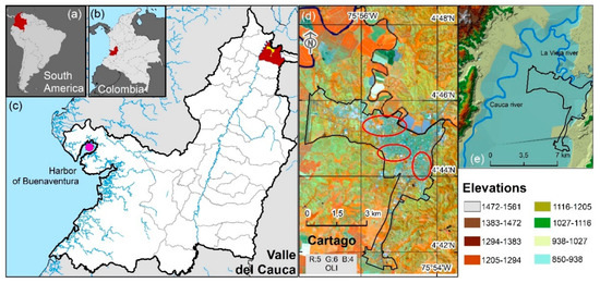
Figure 1.
Location of the study area. (a) South America: Colombia highlighted. (b) Location of Valle del Cauca in Colombia. (c) Cartago in Department of Valle del Cauca. (d) Cartago, Landsat 8 OLI band combination (R:5, G:6, B:4). (e) Digital Elevation Model.
2.2. Data
Data used for the study area (Figure 1a,b) were freely acquired from ESRI World Countries (https://hub.arcgis.com/, accessed on 20 October 2021). The base cartography for the construction of thematic maps and the topographic model is available at https://geoportal.dane.gov.co/, accessed on 20 October 2021 and https://geoportal.igac.gov.co/, accessed on 20 October 2021. The primary information sources used are satellite Earth images from the Thematic Mapper (TM) instrument onboard the Landsat 5 and 7 satellites (L5TM, and L7ETM+), and from the Operational Land Imager (OLI) and Thermal Infrared Sensor (TIRS) onboard the Landsat 8 satellite (L8OLI/TIRS). The images used in this study are sparsely distributed within the period 2001–2020, as shown in Figure 2. Each Landsat product contains separated spectral bands in GeoTIFF format and is referenced to the WGS84 datum in the UTM (18N) cartographic projection. L5TM, L7ETM+ and L8OLI VIS and NIR bands have a spatial resolution of 30 m, while for the TIR satellite instruments, the resolutions are 120, 60, and 100 m, respectively. We employ a total of 37 Landsat scenes (satellite path 009 and row 057) including 2 images of L5TM, 20 of L7ETM+, and 15 of L8OLI/TIRS. In addition to the Landsat products, 11 multispectral Level-2A atmospheric corrected images from the Sentinel-2 Multispectral Instrument (S2-MSI) were also used to extract the so-called Fractional Vegetation Cover (Fcover) biophysical variable. S2-MSI offers a different spatial resolution; the three visible and the near infrared bands have 10 m spatial resolution. The three Red Edge bands, an NIR band, and two SWIR S2-MSI bands have 20 m spatial resolution. These data are very appropriate for the retrieval of geophysical surface parameters. Meanwhile, the three other S2-MSI bands (coastal aerosol, water vapor, and SWIR-Cirrus) have a resolution of 60 m resolution. The reflectance S2-MSI products are freely available on the European Space Agency (ESA) DataHUB server (ESA, https://scihub.copernicus.eu/, accessed on 20 October 2021). Details on the retrieval of Fcover are given in Section 2.3.2. The estimation of LST from the Thermal Infrared Sensor (TIRS) is highly dependent on the intrinsic properties of the coverage, such as the emissivity of the land surface. The emissivity retrieval method based on the Fcover is very suitable due to its ease of application. The performance shown in works such as Sobrino et al. [39] and Valor and Caselles [40].

Figure 2.
Temporal distribution of Landsat and Sentinel 2.
2.3. Methods
The proposed methodology comprises five processing steps: (1) data calibration, (2) extraction of contributing factors, (3) estimation of temperature and emissivity, (4) validation of temperatures, and (5) modeling of the SUHI phenomenon. These are described in the following sections.
2.3.1. Data Calibration
The conversion of image digital values to top of atmosphere radiance (LTOA) was carried out using the gain and offset parameters included in the product metadata file. We use the radiance models provided by the USGS website [41]. Subsequently, the images were corrected from atmospheric effects to minimize the radiance scattering and absorption errors caused by water vapor, dust particles, and aerosols. We employ the Fast Line-of-sight Atmospheric Analysis of Spectral Hypercubes (FLAASH) module of ENVI®, which incorporates the MODerate Resolution Atmospheric TRANsmission (MODTRAN) model [42]. Given the geographic location of the area of interest, the tropical atmospheric model is applied to the Landsat products. FLAASH solves the radiative transfer equation by determining the water vapor for each pixel in the image. Water vapor content (WVC) retrieval is not a straightforward solution for Landsat bands, so this parameter was taken from a standard atmospheric model. Regarding the aerosol concentration or aerosol optical depth (AOD), the dark vegetation reflectance algorithm of Kaufman et al. [43] was applied. Finally, all images were subset to fit the boundaries of the study area.
2.3.2. Definition and Extraction of Contributing Factors
Spectral indices such as NDBI, NDVI, and NDWI are used to examine the underlying properties of SUHI formation. Analytical expressions of these indices can be found in Zha et al. [44], Tucker [45], and Gao [46]. Moreover, the components of the tasseled cap (TC) components (brightness, greenness, and wetness) are also computed [47]. The rationale for the selection of these biophysical indices is as follows.
- Energy exchange between latent and sensible heat is related to NDBI, since it detects impervious surfaces that reduce humidity and increase the average temperature of the environment [48].
- Temperature and vegetation maintain a spatially dependent relationship [49]. Vegetation reduces surface irradiation and increases humidity through physiological processes that allow energy exchange, while producing a cooling effect. In this sense, an index for measuring this photosynthetic activity is the NDVI.
- The presence of water bodies has a cooling effect on urban temperature [50]. In this scheme, the NDWI quantifies the water content in the vegetation, while suggesting a significant effect in reducing SUHI. Likewise, rivers play an important role as thermal regulators of urban climate, increasing the cooling potential through evaporation and facilitating airflow. Given that the urban center is the main point for the development of socioeconomic activities, two additional variables were considered to describe the expression of the proximity, i.e., the proximity map of the water body (PW) and the proximity map (PW) and the city center (PUC). A greater distance would imply a lower thermal intensity [51]. The proximity indices are computed by means of a Euclidean distance using the inverse weight distance operator in ArcGIS® (https://esri.com/, accessed on 20 October 2021).
The above indices conform to the contributing factors to our proposed SUHI model. To compute the emissivity values required to retrieve LST from Landsat thermal bands, a novel method is proposed through extracting Fcover biophysical variable, although this information can be derived indirectly from NDVI, Leaf area index (LAI), or other biophysical variables [52,53,54]. Bacour et al. [55] proposed a robust procedure based on the Neural Network training of the PROSAIL (PROSPECT leaf optical properties model and SAIL canopy bidirectional reflectance) model. This Fcover variable is implemented in the ESA’s Sentinel Application Platform (SNAP (https://step.esa.int/main/toolboxes/snap/, accessed on 20 October 2021), and requires S2-MSI images. Detailed descriptions of this scheme are available in Weiss and Baret [56]. The Fcover variable provides the emissivity values necessary to compute LST with the L8OLI/TIRS thermal band 10. Compared to traditional methods based on NDVI, this new approach for extracting the emissivity is suitable for thermal radiation models. Due to temporal synchronization between S2-MSI and L8OLI/TIRS images, this method is only applicable since 2015.
2.3.3. Estimation of Land Surface Temperature and Emissivity
Land surface temperatures are retrieved from L5TM, L7ETM+, and L8OLI/TIRS. For L8OLI/TIRS, only band 10 is used, since band 11 has large uncertainties, as reported by the USGS [57]. The consistency of Landsat 5, 7 and 8 satellite thermal instruments in recovering LST was compared by Sekertekin and Bonafoni [58] and validated with in situ LST measurements. The RMSE values were 2.39 °C, 2.57 °C and 2.73 °C, respectively, resulting in an average difference of 0.2 °C between the sensors. The uncertainty values are adequate uncertainty for the purpose of this study. In Figure 3, our model to retrieve LST is presented in a flow chart. Temperatures are derived using the radiative components implemented by Barsi et al. [59] for single-channel algorithms. This method simulates the attenuation effects of the atmosphere that disturb the TIR signal.
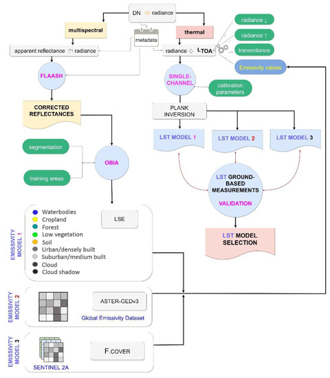
Figure 3.
Flowchart for LST estimation and assessment of the emissivity models used in this study.
Radiance and transmissivity values are available at https://atmcorr.gsfc.nasa.gov/, accessed on 20 October 2021. The data is a compendium of atmospheric transmissivity values, along with upwelling and downwelling radiances for a given geographical location. The radiative values can be used in atmospheric correction models, e.g., Equation (1), taking also into account the correction of spectral emissivity.
In this equation, is the spectral radiance at the top of the atmosphere (registered by the sensor), is the atmospheric transmittance, is the spectral emissivity, is the spectral radiance of a black-body target of kinetic temperature T, and are the upwelling atmospheric path radiance and the downwelling or sky radiance, respectively.
Implementing Equation (1) requires the supply of adequate emissivity values for a suitable estimation of LST. Since different land covers emit thermal radiation differently, spectral emissivity corrections are necessary [60]. In this work, three emissivity models are tested to accurately estimate LST. First, the field-measured LSE (land surface emissivity) values are obtained from different authors, and are listed in Table 1. Then the emissivity data of the ASTER-GEDv3 product [61] were considered.
Then, the Fcover model of Valor and Caselles [40] is applied; this model allows the calculation of the emissivity in the Landsat 8 thermal band, considering the Fcover index and the minimum and maximum values of the emissivity in the corresponding spectral band. Finally, the three LST models are compared and validated. In this study, land use features are categorized into seven classes. These are water bodies, cropland, forest, low vegetation, bare soil, urban/densely built, and suburban/medium built. We applied this scheme following the land cover classes proposed by Park et al. [62]. Since impervious surfaces exhibit a large spectral variation [63], two classes are used to represent artificial surfaces: urban/dense and suburban/medium. These classes are particularly identified by the impact on emissivity.
For this purpose, an object-based classification is carried out using Trimble’ s eCognition Developer software (https://geospatial.trimble.com/products-and-solutions/ecognition, accessed on 20 October 2021).

Table 1.
Reference values for the LSE model with L8OLI/TIRS band 10.
Table 1.
Reference values for the LSE model with L8OLI/TIRS band 10.
| Land Cover | Emissivity | Reference |
|---|---|---|
| Waterbodies | 0.992 | FROM-GLC cited by [64] |
| Cropland | 0.971 | FROM-GLC cited by [64] |
| Forest | 0.995 | FROM-GLC cited by [64] |
| Low vegetation | 0.986 | Tan et al. [65] |
| Soil | 0.972 | Tan et al. [65] |
| Urban/densely built | 0.973 | FROM-GLC cited by [64] |
| Suburban/medium built | 0.971 | Tan et al. [65] |
The second emissivity dataset in this work is the ASTER Global Emissivity Dataset v3 (ASTER-GEDv3) [61], (https://emissivity.jpl.nasa.gov/aster-ged, accessed on 20 October 2021). This method was developed by the NASA Jet Propulsion Laboratory (JPL) as an algorithm based on temperature and emissivity separation along with an atmospheric correction model. More details can be found in Hulley and Hook [66].
The third emissivity model requires knowledge of the Fcover variable [40]. This method provides the emissivity of a heterogeneous surface as follows:
In this equation, and are reference vegetation and bare soil emissivity, respectively. ‘’ is the cavity effect associated with the indirect radiance emitted due to internal reflections between the interfaces. Here, Fcover is obtained from S2-MSI Level 2A products (see Section 2.3.2). The procedure to retrieve the Fcover variable differs from the NDVI methods [67,68], and is presented as a novel alternative for thermal modeling with Landsat data. In tropical areas, throughout the year, vegetation dynamics does not exhibit abrupt changes, and this implies that Fcover lacks significant seasonal variations. For the L5TM and L7ETM+ thermal instruments, the emissivity model of Equation (3) [69] is used. This last method to obtain Fcover is based on the NDVI parameter.
In this equation, and are the reference emissivity values for nonvegetated and vegetated areas, being 0.97 and 0.99, respectively [70]. In this work, the Fcover variable is recovered using the NDVI, as it effectively reflects the conditions of vegetation cover [42]. This is estimated by Equation (4).
In this equation, is the NDVI value of pure soil, and is the NDVI of pure vegetation obtained from the NDVI image.
This method is based on the Carlson and Ripley [69] model. Finally, the conversion from LTOA to LST is estimated by using the constants for sensor calibration and the inversion of the Planck equation [71].
2.3.4. Assessment of the Land Surface Temperature Retrieved from L8TIRS B10
Landsat-retrieved LST was verified with in situ measurements. Unfortunately, due to the Landsat overpasses schedule, starting in 2001, it was impossible to undertake a validation by means of field surveys for the entire Landsat time series. Due to these inconveniences, the comparison was limited only to two overpasses of L8OLI/TIRS band 10. The L5TM and L7ETM+ data, the Carlson and Ripley results [69] can be used as a reference. In situ temperatures were measured using 30 thermometers assembled into DS18B20 digital sensors. The direct calibration method was applied, which consists in recording the readings of the test and standard thermometers. The latter are preserved in an isothermal medium. This calibration procedure produced standard deviations of ±0.5 °C. The field survey consists of distributing 30 devices, as shown in Figure 4. LST measurement coincident with the two L8OLI/TIRS overpasses were recorded on 22 January and 9 September 2019. Each device recorded the temperature values by means of a probe in contact with the ground surface. The ground sensors were placed in areas with homogeneous land cover to minimize the spatial thermal variation caused by different emissivity values. These records will be used to contrast the LST values derived from satellite measurements. In Section 3.1, we perform a sensitivity analysis for the three emissivity models.

Figure 4.
Location of in situ ground LST measurements.
2.3.5. Modelling the SUHI Phenomenon
According to Rasul et al. [72], SUHI modeling consists of identifying the spatial variation in time of thermal features in urban areas. Here, through the combination of thermal images from remote sensing and sparse measurements on field, our SUHI model employs the PCA to analyze space-time data. The PCA is a multivariate statistical technique that preserves the total variance of a dataset while reducing its dimensionality [73]. In this way, the PCA can retrieve the main spatial patterns of variability in a time-series. The application of PCA provides a generalization of the changes that characterize the variability patterns in a time series of images [18].
Then, the impacts of the eight factors considered in this study are assessed using a MLR approach. The MLR technique is a parametric model that adjusts the relationship between explanatory variables, that is, the contributing factors, and the response variable, e.g., LST. The inclusion or elimination of predictors depends on the significance of these variables within the model, which is defined by a test hypothesis based on the coefficients associated with the response variable. When using MLR techniques, it is important to examine the key assumptions of autocorrelation, normality of residuals, and multicollinearity. These factors determine the reliability of the model [74]:
- Autocorrelation of a variable represents its self-dependence and implies redundant information that makes the estimator lose efficiency. The Durbin-Watson statistic is used to measure autocorrelation [75].
- The normality of a residuals guarantees a satisfactory representation of the model.
- Multicollinearity occurs when the predictor variables are highly correlated. Multicollinearity increases the variance, causing instability of the regression and thus increasing the standard error [76]. Multicollinearity is measured with the Variance Inflation Factor (VIF).
Finally, outliers can also alter the modelling approach, causing problems with regression assumptions [77,78], and these must be controlled or removed from the dataset. Here, our MLR analysis is an equation capable of describing the thermal intensity depending on the contributing factors. To verify the relative importance of each individual predictor of the LST model, a normalization procedure was previously performed to standardize the coefficients. We use the deviation of the mean values, which is divided by the standard deviation of the response variable in LST. This allows us to derive the standardized coefficients [79]. Subsequently, the contribution of each variable to LST is obtained by weighting the absolute value of each variable. The resulting weights are further used for assessing the subsequent Machine Learning procedure that derives the multitemporal intensity of the SUHI model. This provides a technical basis for analyzing the factors that influence the thermal environment, which is of great significance for rational urban planning and sustainability.
The methodological workflow in Figure 5 shows the spatiotemporal model followed to characterize the impact of environmental factors on the thermal changes. First, the multitemporal factors, such as LST, spectral indices, and other variables, are derived from the Landsat 2001–2020 dataset. Then, the PCA technique is applied to extract the main patterns of variability. Subsequently, all the variables involved are included in the MLR scheme to model the possible dependences on LST. The MLR is implemented with the software R Studio (https://rstudio.com/, accessed on 20 October 2021).
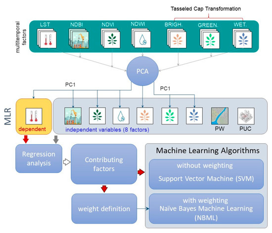
Figure 5.
Flowchart of the proposed SUHI model.
Finally, the SUHI phenomenon is segmented into different zones depending on the thermal intensity. Thermal value ranges follow the categories of Wang et al. [36], which consider the average temperature of the land surface and its standard deviation (SD). Segmentation provides a definitive SUHI product that categorizes the urban environment according to specific conditions. Here we test two different Machine Learning methods for classification; Support Vector Machine (SVM) and Naïve Bayes Machine Learning (NBML). Both SVM and NBML methods have shown in previous research their robustness for the characterization of various types of geospatial data [80,81]. The SVM method defines a separate hyperplane in a higher-dimensional space that optimally classifies the data. This method is particularly useful for solving nonlinear relations [82], and is available as open-source software in Orfeo ToolBox (OTB) at https://www.orfeo-toolbox.org/, accessed on 20 October 2021. The NBML technique is based on the Bayes theorem for conditional probability and assumes independence between predictors, variables, or features [83].
NBML is often referred to as the maximum a posteriori decision rule [84], and its code can be easily written in any programming language. NBML assigns the most likely class to a certain observation by estimating the probability density of the training classes [85]. An observation is classified as a certain class when the posterior probability reaches the maximum value according to the following expression:
In this equation, is the maximum a posteriori of for the class labeled as , is the prior probability for class represents the conditional probability distribution of given , and is a particular weight applied to each factor. Usually, the independence assumption is not fulfilled, and the weighting of the features involved in the assignment process can satisfy the required assumptions [86]. Here, each feature or factor is affected by a particular weight , which can be formally defined by:
In this equation, denotes the weight value of the ith attribute, with values restricted to the range [0, 1]. In this work, attributes are the contributing factors involved in the SUHI phenomenon, while the classes are the seven temperature categories defined by Wang et al. [36]. These are described in Table 2.
Table 2.
Range of LST intervals. Ts represents land surface temperature; Ta is the average land surface temperature. SD is the standard deviation.
The prior and conditional probabilities are determined through a training process. Then, Equation (6) becomes:
In this equation, and are estimates of the probabilities density functions (PDFs). These are derived from the frequency of their respective arguments in the training sample. Here, can also be estimated from a preliminary outcome of a SVM process.
Equation (7) allows us to weight each environmental factor to generate the final SUHI product. The resulting map is generated according to the architecture shown in Figure 6, which is based on the NB decision rule. This approach categorizes the urban environment according to a specific condition and assigns a specific type of action based on each temperature category. This analytical procedure allows one to obtain a map that delimits the areas of different thermal intensities. The resulting areas are based on the spatiotemporal trends of the contributing factors, facilitating the management and application of measures to mitigate/adapt the SUHI phenomenon.
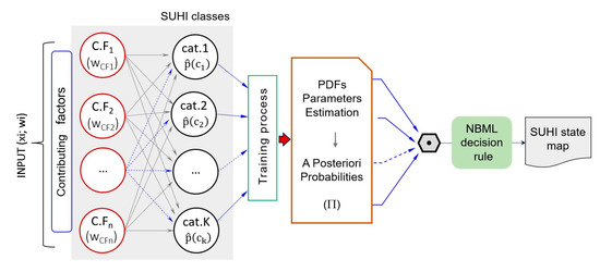
Figure 6.
Architecture of the NBML modelling for generating the SUHI product.
3. Results
3.1. Land Surface Temperature
Sensitivity analysis of the three emissivity models is performed prior to retrieving land surface temperatures from the 37 Landsat images; the results of the assessment for the LST retrieved from L8/TIRS B10 (described in Section 2.3.4) are presented here. Figure 7 shows the differences between LST derived from the three models evaluated in this study (Fcover, AS-TER-GEDv3, and LSE), and these are compared with in situ LST. In this figure, the minimum, maxima, median and mean values are shown for (a) January 2019 and (b) September 2019. In both cases, the lowest differences agree with the LST values from our Fcover emissivity model.
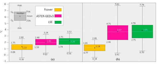
Figure 7.
Boxplots of LST results from Fcover, ASTER-GEDv3, and LSE. The white horizontal line in each box is the median. (a) January 2019; (b) September 2019.
The interquartile ranges show a narrower dispersion for the Fcover model compared to the ASTER-GEDv3 and the LSE model. This feature is obvious for the campaign in September 2019. The regression analysis between the LST from ground-based sensors and that of the L8OLI/TIRS band 10 is shown in Figure 8. The dark gray areas represent the confidence boundaries of 95%, while the solid lines represent the line of best fit between the computed and in situ LST. The best determination coefficient is given by Fcover with R2 = 0.78 and SD = 0.73 °C (Figure 8a). For the other two cases, the coefficients are R2 = 0.27 and R2 = 0.26 for the ASTER-GEDv3 and LSE models, respectively.
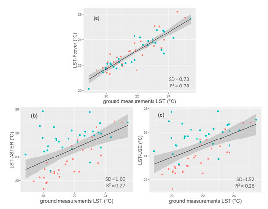
Figure 8.
Regression analysis between LST from L8OLI/TIRS and that from ground measurements. Color code: Orange, January; Green, September (a) Fcover; (b) ASTER-GEDv3; (c) LSE model.
3.2. Principal Component Analysis
The PCA was carried out using all contributing factors during the period 2001–2020 (37 images for each variable). Figure 9 shows the contribution to the total variance of each PCA component. We can observe that the first PCA component (PCA1) of T-cap Brightness and T-cap Wetness provide a lower contribution to the total variance, with 54% and 64%, respectively. On the other hand, the rest of the variables show larger patterns of variability with only the first PCA component (above 75%).
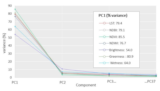
Figure 9.
Contribution of the main PCA components to the total variance for the different variables used in this study.
Regarding the explained variance (%) of the second principal component or the T-cap Brightness, it is observed that it still retains a large amount of variance (12%), when compared to other factors. Since the goal of the PCA is to reduce the set of variables, in the case of the T-cap Brightness, the former dataset cannot be strictly explained by the first principal component, as it is the case of the remaining factors. This implies that further analysis is addressed towards investigating the second or even third components of the T-cap Brightness.
We employ the Jenks Natural Breaks grouping model [87] to identify the main groups and the inherent patterns that minimize the deviation of each class with respect to the mean value of the other groups. This method reduces the variance within the classes and maximizes the variance between classes. In this scheme, we obtain four groups for each factor, representing the spatiotemporal trends between 2001–2020. Figure 10 shows the resulting maps where the results for LST (Figure 10a) show the maximum concentration of temperature in densely populated areas, similar to the results of NDBI (Figure 10b). The LST results show gradual variations from low to high temperatures near the perimeter of urban areas. Regions with lower temperatures are mainly located in areas close to water bodies and dense vegetation. Vegetation areas can be identified in the NDVI results (Figure 10c). The NDVI and T-Cap Greenness maps Figure 10c,f have high similarity, while the T-Cap Brightness and Wetness maps Figure 10e,g lack spatial correlation with the thermal phenomenon. In the next section, we analyze the spatial correlations in more detail.

Figure 10.
First PCA components for the main factors during the period 2001–2020: (a) land surface temperature; (b) normalized difference built-up index; (c) normalized difference vegetation index; (d) normalized difference water index; (e) T-cap brightness; (f) T-cap greenness; (g) T-cap wetness.
3.3. Multiple Linear Regression
A large number of outliers were identified and removed in the brightness and humidity factors to avoid introducing “noise” into the MLR analysis. All residuals greater than 3σ standard deviation from the mean value are considered outliers and thus removed. Since NDVI and Greenness factors are highly redundant (R2 = 0.99), the latter was excluded. Concerning the Brightness factor, under the special circumstances observed in Section 3.2, the two first principal components only explain 66% of the total variance. Moreover, the low spatial correlation with LST (Figure 10) suggests excluding this variable.
Then, in the Fisher hypothesis test for the PW factor is larger than 0.1, and it was removed. Finally, the scrutiny explanatory variables are NDBI, NDVI, NDWI, and PUC, and the resulting MLR model outcomes as follows:
The regression analysis coefficients are shown in Table 3. In this table, p (>|t = 0.05|) represents the probability of observing any value larger than t. In our model, all p-values are below the significance level (0.05). This implies that NDBI, NDVI, NDWI and PUC are statistically significant predictors. The model has a high coefficient of determination (R2 = 0.82), this means that these variables explain 82% of the variability observed in the LST.
Table 3.
Multiple Linear Regression coefficients.
The p-values of the regression analysis are shown in Table 3. All p-values are smaller than 0.05, indicating that the relationships between independent and dependent variables are statistically significant. Finally, to support the validity of the model, the following key assumptions were verified: autocorrelation, normality, and multicollinearity. The resulting values are given in Table 4.
Table 4.
Fulfillment of the Assumptions.
In this table, we can appreciate that the NDBI and NDWI VIF values are greater than 10, thus exceeding the tolerance. This implies that these two variables should be disregarded. As stated by Szymanowski and Kryza [88], the variables that exceed this tolerance may be considered to improve a regression model. Moreover, these two predictors are very important variables in many UHI studies [89,90,91]. In the UHI study by Cruz et al. [92], after performing a multicollinearity test, explanatory variables with VIFs between 50 and 70 were selected for their multiregression analysis. These were considered an important component for modeling this phenomenon. These are the reasons for maintaining the NDBI and NDWI as explanatory variables in this study.
The independence between residuals was verified using the Durbin–Watson statistic (D-W) with a value of 2.0, which falls within the critical values of 1.5 < D-W < 2.5, indicating the absence of autocorrelation. The normality of the residuals was proved by applying a Kolmogorov–Smirnov (K-S) test, which confirms the normal distribution. Figure 11 shows the scatter diagrams, the histograms, and the correlation values for each pair of explanatory variables in the model. To verify our model assumptions, four scatterplots of residuals against fitted values are investigated. Figure 12 suggests that the data are randomly distributed around zero, with constant variability. There are no patterns that indicate that the assumptions of the model are fulfilled for the dataset.
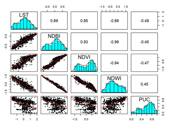
Figure 11.
Histograms of the model variables (i.e., LST, NDBI, NDVI, NDWI, and PUC) in the main diagonal. Scattergrams between the model variables (below main diagonal), and the corresponding Pearson correlation (above main diagonal).
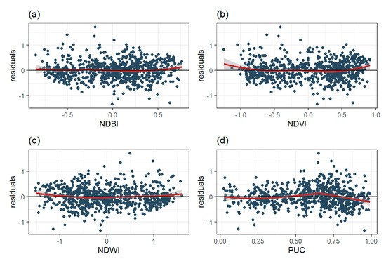
Figure 12.
Performance of the linearity of the model. Graphs of the regression analysis residuals vs. fitted lines. (a) NDBI vs. residuals. (b) NDVI vs. residuals. (c) NDWI vs. residuals. (d) PUC vs. residuals.
In this figure, good correlation of NDBI and NDWI with LST is observed.
The contribution of each variable () was obtained through the standardized regression coefficients (), which are weighted means absolute value. The resulting standardized regression coefficients and the contribution of the factors to the model are presented in Table 5. In this table, we can observe that the main contributing factors are the variables NDWI and NDBI, followed by NDVI and PUC. The derived weights are used in the next section to derive the SUHI model.
Table 5.
Standardized Regression Coefficients and Contribution of each Factor.
3.4. SUHI Modeling
The SUHI phenomenon depends on the properties of land cover properties which, combined with their energy absorption capacity, produce a thermal increase on the surface and represent a threat to the thermal regime of urban ecosystems. Our modeling approach is based on segmentation through the identification of potential thermal areas. Here we employ the seven temperature zones defined by Wang et al. [36]. The definition of the training areas is achieved with the LST variable (Figure 10a). The thermal ranges for the training process are those defined in Table 2. These ranges are based on LST averages and the standard deviations. We test both the SVM and NBML algorithms. The application of the NBML method requires estimating the conditional probability functions for each contributing factor. The Gaussian and Logistic probabilities density functions showed the best results for the respective training frequencies of observation/category. Each conditional probability was weighted according to Table 5. Moreover, the weighting capability of the NBML method allows taking into account the relevance of each factor for deriving the SUHI product. This feature is not possible with the SVM method.
The segmentation results for both methods are shown in Figure 13. In both cases, the results were validated with the criteria established in Table 2. Table 6 reports the Kappa index for SVM and NBML are approximately 88% and 94%, and the overall accuracy are 88% and 95%, respectively.
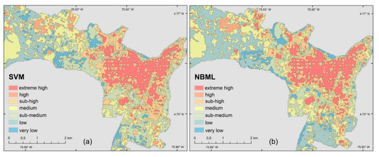
Figure 13.
Temperature classification results. (a) SVM; (b) naïve Bayes.
Table 6.
Kappa Index and Precision of SVM and NBML.
Figure 13 and Figure 14 show the final SUHI map that categorizes the urban environment according to a specific SUHI state and assigns a specific type of action based on temperature. The proposed actions are: intervene, monitor, strengthen, and preserve. The intervene action is directly related to the SUHI areas exposed to the maximum thermal concentration. These areas need to be immediately intervened in and are considered an ‘Extreme-high’ class. The monitor action groups ‘High’ and ‘Sub-high’ categories, and points to the SUHI areas that should be kept under observation and intervened in a medium term. The strengthen action classifies the ‘Medium’ and ‘Sub-medium’ classes into SUHI areas that have gradually presented a temporary thermal trend increase. The preserve action contains the ‘Low’ and ‘Very-low’ classes and comprises the SUHI areas that must be preserved.

Figure 14.
Final SHUI product from NBML. The legend recommendations are specific types of action based on temperature warnings.
4. Discussion
4.1. Sensitivity Analysis
The results of the January 2019 campaign (Figure 7a) suggest that the amplitude of the errors in recovering LST is similar between the models evaluated. The September 2019 measurement records (Figure 7b) indicated that the Fcover model provides the smallest deviation with a mean error of 1.14 °C. This is very obvious compared to ASTER-GEDv3 and the LSE model, which shows mean deviations of 3.67 °C and 3.85 °C, respectively. As shown in the Results section, the Fcover model exhibited better performance with a mean error of 1.33 °C. Data reported by Duan et al. [93], and Malakar et al. [94] showed differences for L5TM, L7ETM+, and L8OLI/TIRS among recovered LST and in situ LST between 0.7 and 1.2 °C. Furthermore, we observed mean differences between 1.1 °C and 1.3 °C. Authors such as Chen and Zhang [14] and Liu and Li [95] have analyzed the SUHI phenomena with similar differences. In this work, the Fcover model provided the smallest errors in LST recovery among all the tested schemes, and it is considered the most suitable for this kind of studies.
4.2. Statistical Analyses
The PCA was applied to derive the time trend of each variable and to analyze the LST variation. Then, the main PCA component was employed in the MLR. We achieve a coefficient of determination of approximately R2 = 0.82. These results are in agreement with recent studies that have used regression models to quantify the impact of contributing factors on LST [16,96]. Moreover, the combination of these factors defines how the different types of land cover absorb temperatures. These absorptions manifest themselves with the corresponding increase in emissivity and surface temperature. Our findings confirm results of earlier studies, such as those of Rasul et al. [72], who modeled with the MLR method the spatiotemporal trend of temperature data, and provided robust results in determining SUHI areas.
Regarding the conditions for ensuring the validity of our proposed approach, several considerations must be addressed. First, the multicollinearity of the predictor variables and their effect on the model need to be validated with the VIF. Our results show that two of the VIF parameters exceeded the value of 10, which would exclude two of the explanatory variables of the prediction model. However, it is found that NDBI and NDWI are the factors with the highest contribution, while NDVI and PUC have lower VIF values, contributing to a lesser extent. Strong correlations, 0.89 and −0.89, were found between the LST and NDBI and NDWI, respectively. A similar correlation was found between NDVI and NDWI. It is important to note that removing highly correlated variables can benefit the overall result and simplify the approach. However, having high contributing predictor variables such as NDBI and NDWI may indeed improve prediction products, as noted in [88]. Although some collinearity was presented, the Pearson correlation indices and the fulfillment of independence and normality of the residuals have denoted a very reliable model.
Regarding the direct relationships of LST with the different physical variables and contributing factors, a strong correlation with NDBI was observed: building construction. This justifies why impervious areas have high caloric retention capacity and low water storage capacity, in turn reducing humidity. Previous studies have demonstrated strong correlations between LST and NDBI [97,98]. In contrast, a strong correlation was found between LST and NDVI/NDWI. Please note that temperature decrease follows increases in vegetation and humidity. The higher the vegetation cover, the lower the surface temperature becomes. The reason for this may be strongly related to the soil moisture content in vegetated areas, which alters the energy balance and causes variation effects from solar radiation. These results are in line with those obtained by Ibrahim and Rasul Faqe [99], who reported a strong negative correlation between these variables. Our results show urban planners that the identification of factors and their contribution to the SUHI phenomenon serves as a support to define adaptation measures to cities for thermal change, allowing them to adapt with other territorial planning priorities.
A moderate correlation was found between LST and PUC, indicating that LST increases moderately according to the proximity to the urban center. This correlation may be related to urban density distribution and road infrastructure, which, compared to the distance variable, are responsible for generating a complex structure not well represented by linear models. Bonafoni and Keeratikasikorn [100] also implemented a ring-based method and analyzed LST as a function of building density and proximity to urban centers. This issue is to be addressed in future research.
4.3. The SUHI Model
To reveal the multitemporal intensity of the SUHI phenomenon, two Machine Learning techniques were tested, the SVM and the NBML. Both algorithms performed satisfactorily, with Kappa indices of 89% and 93%, respectively. Better performance was observed for certain categories for the NBML algorithm (Figure 13b). Although both procedures are able to detect high-density urban areas affected by extremely high temperatures, NBML allows coupling criteria to assign individual weights to each class, increasing the quality of the results. Conventional NBML classifiers consider the model to be applicable when the Gaussian probability density function is present in the data set [84]. Molina et al. [101] showed that the combination of the best-fit distribution model (not necessarily Gaussian), and the weights of each variable led to satisfactory results.
The SUHI phenomenon is a complex system that occurs as a result of the interaction of various factors [102]. This interactivity produced by anthropic effects generates thermal imbalances requiring intervention, monitoring, strengthening, and preservation, as a fundamental expression between causes and effects of urban/rural ecosystems. Our results show that the highest temperatures are concentrated in the central area of the city and gradually decrease toward the periphery. The characterization of the space through the four proposed classes of actions (intervene, monitor, strengthen, and preserve) makes it possible to regulate the conditions that could mitigate the SUHI effect. The areas designated as intervene correspond to the center of the city and tend to have a higher population density and old buildings. It is recommended to change black roofs to less thermic roofs that have reduced solar energy absorption and increased energy savings, as suggested by Alshayeb and Chang [103]. Since these areas do not have appropriate physical space to create green areas, an alternative might be the use of road dividers to plant trees with large foliage and roots that do not weaken existing infrastructure. An interesting measure that allows the reduction of anthropogenic heat is to restrict the transit of private vehicles and limit access to specific areas. The access methods can be substituted for public transportation or cycling. These measures have already been implemented in many locations. The areas identified as monitor should implement small tree-lined sites and natural corridors to refresh the space. Rainwater irrigation channeled through sewerage systems can be used as a contribution to the restoration of urban wetlands. The areas indicated as strengthen show less thermal intensity than the above areas and are associated with urban growth. Within this policy, the morphology of these areas should integrate green spaces that allow increased water infiltration and cooling [104]. In general, the use of highly reflective building materials is recommended, reducing the amount of solar radiation absorbed by the surface, such as, for example, the use of cool pavements suggested by the U.S. Environmental Protection Agency [105]. Finally, areas marked as preserve have the highest vegetation cover and play an important role in the urban ecosystem. They reduce carbon dioxide emissions, becoming spaces that reduce the radiant load produced by various economic activities, and generate thermal regulation. In addition, these have a great potential for ecotourism.
Further development of this research can be undertaken by applying simulation techniques with Machine Learning Algorithms that allow the integration of weights to the variables involved in the predictive model, and that allow characterization of future thermal scenarios associated with the spatiotemporal trends of the explanatory variables. The interactions produced by biophysical factors and the geometric changes that are transforming cities make the relationships between objects and phenomena increasingly complex. In this sense, it would be very pertinent to further explore the classification of local climatic zones in tropical cities in countries such as Colombia. These are highly vulnerable to climate change.
5. Conclusions
The results of this work demonstrate that emissivity data have a large impact on the retrieval of LST. Here, LST is obtained from L8OLI/TIRS band 10 and LSE from Sentinel-2. Both sources are more accurate and homogeneous than using traditional ground-based methods. Our innovative approach proposes quantifying the SUHI phenomenon from a set of contributing factors. We first employ the PCA to retrieve the main spatiotemporal variations in the initial data. Then, MLR is applied to integrate the dependencies and to analyze their impacts on SUHI. According to our regression model, the most influential factors in the SUHI are NDWI with a contribution of 52%, NDBI with 21%, NDVI with 13%, and PUC with a 14%. Finally, the integration of these predictors within an SVM and a NBML approaches confirms the existence of coupling mechanisms between each variable. The satisfactory results of the NBML confirm the suitability of the proposed approach, with an overall accuracy of 95%. We expect to improve the results of the model with future upgrades associated with structural complexity of the landscapes. The spatial variation of SUHI points out an enhanced phenomenon towards areas of high urban density. Our research demonstrates the suitability of Machine Learning Algorithms for mapping SUHI intensities, providing spatially explicit descriptions of urban heat distribution. The derived products are crucial for defining sustainable urban planning policies, as well as for adequate responses to thermal risks. These actions will in turn make it possible to define mitigation and adaptation strategies.
Author Contributions
J.G. and I.M. provided the main ideas, developed the methodology model, conceived and performed the comparison experiments, and analyzed the results. Both of them contributed equally. A.C. performed manuscript editing and revision tasks. J.V. supervised the whole process and reviewed the manuscript. All authors have read and agreed to the published version of the manuscript.
Funding
This research received no external funding.
Institutional Review Board Statement
Not applicable.
Informed Consent Statement
Not applicable.
Data Availability Statement
The data presented in this study are available on request from the corresponding author.
Conflicts of Interest
The authors declare no conflict of interest.
References
- Oke, T.R. The energetic basis of the urban heat island. Q. J. R. Meteorol. Soc. 1982, 108, 1–24. [Google Scholar] [CrossRef]
- Voogt, J.A.; Oke, T.R. Thermal remote sensing of urban climates. Remote Sens. Environ. 2003, 86, 370–384. [Google Scholar] [CrossRef]
- Schwarz, N.; Schlink, U.; Franck, U.; Großmann, K. Relationship of land surface and air temperatures and its implications for quantifying urban heat island indicators—An application for the city of Leipzig (Germany). Ecol. Indic. 2012, 18, 693–704. [Google Scholar] [CrossRef]
- Gubler, M.; Christen, A.; Remund, J.; Brönnimann, S. Evaluation and application of a low-cost measurement network to study intra-urban temperature differences during summer 2018 in Bern, Switzerland. Urban Clim. 2021, 37, 100817. [Google Scholar] [CrossRef]
- Chakraborty, T.C.; Lee, X.; Ermida, S.; Zhan, W. On the land emissivity assumption and Landsat-derived surface urban heat islands: A global analysis. Remote Sens. Environ. 2021, 265, 112682. [Google Scholar] [CrossRef]
- Sobrino, J.A.; Oltra-Carrió, R.; Sòria, G.; Jiménez-Muñoz, J.C.; Franch, B.; Hidalgo, V.; Mattar, C.; Julien, Y.; Cuenca, J.; Romaguera, M.; et al. Evaluation of the surface urban heat island effect in the city of Madrid by thermal remote sensing. Int. J. Remote Sens. 2013, 34, 3177–3192. [Google Scholar] [CrossRef]
- WMO Essential Climate Variables. Available online: https://public.wmo.int/en/programmes/global-climate-observing-system/essential-climate-variables (accessed on 18 October 2019).
- Zhou, D.; Xiao, J.; Bonafoni, S.; Berger, C.; Deilami, K.; Zhou, Y.; Frolking, S.; Yao, R.; Qiao, Z.; Sobrino, J.A. Satellite remote sensing of surface urban heat islands: Progress, challenges, and perspectives. Remote Sens. 2019, 11, 48. [Google Scholar] [CrossRef] [Green Version]
- Sekertekin, A.; Zadbagher, E. Simulation of future land surface temperature distribution and evaluating surface urban heat island based on impervious surface area. Ecol. Indic. 2021, 122, 107230. [Google Scholar] [CrossRef]
- Li, S.; Zhao, Z.; Miaomiao, X.; Wang, Y. Investigating spatial non-stationary and scale-dependent relationships between urban surface temperature and environmental factors using geographically weighted regression. Environ. Model. Softw. 2010, 25, 1789–1800. [Google Scholar] [CrossRef]
- Mei, C.-L.; Wang, N.; Zhang, W.X. Testing the importance of the explanatory variables in a mixed geographically weighted regression model. Environ. Plan. A 2006, 38, 587–598. [Google Scholar] [CrossRef]
- Senanayake, I.P.; Welivitiya, W.D.D.P.; Nadeeka, P.M. Remote sensing based analysis of urban heat islands with vegetation cover in Colombo city, Sri Lanka using Landsat-7 ETM + data. Urban Clim. 2013, 5, 19–35. [Google Scholar] [CrossRef]
- Bokaie, M.; Zarkesh, M.K.; Arasteh, P.D.; Hosseini, A. Assessment of Urban Heat Island based on the relationship between land surface temperature and Land Use/Land Cover in Tehran. Sustain. Cities Soc. 2016, 23, 94–104. [Google Scholar] [CrossRef]
- Chen, X.; Zhang, Y. Impacts of urban surface characteristics on spatiotemporal pattern of land surface temperature in Kunming of China. Sustain. Cities Soc. 2017, 32, 87–99. [Google Scholar] [CrossRef] [Green Version]
- Hereher, M.E. Effect of land use/cover change on land surface temperatures—The Nile Delta, Egypt. J. Afr. Earth Sci. 2017, 126, 75–83. [Google Scholar] [CrossRef]
- Shi, Y.; Xiang, Y.; Zhang, Y. Urban design factors influencing surface urban heat island in the high-density city of guangzhou based on the local climate zone. Sensors 2019, 19, 3459. [Google Scholar] [CrossRef] [PubMed] [Green Version]
- Song, J.; Wang, J.; Xia, X.; Lin, R.; Wang, Y.; Zhou, M.; Fu, D. Characterization of urban heat islands using city lights: Insights from modis and viirs dnb observations. Remote Sens. 2021, 13, 3180. [Google Scholar] [CrossRef]
- Parmentier, B. Characterization of land transitions patterns from multivariate time series using seasonal trend analysis and principal component analysis. Remote Sens. 2014, 6, 12639–12665. [Google Scholar] [CrossRef] [Green Version]
- Firozjaei, M.K.; Alavipanah, S.K.; Liu, H.; Sedighi, A.; Mijani, N.; Kiavarz, M.; Weng, Q. A PCA-OLS model for assessing the impact of surface biophysical parameters on land surface temperature variations. Remote Sens. 2019, 11, 2094. [Google Scholar] [CrossRef] [Green Version]
- Lemus-Canovas, M.; Martin-Vide, J.; Moreno-Garcia, M.C.; Lopez-Bustins, J.A. Estimating Barcelona’s metropolitan daytime hot and cold poles using Landsat-8 Land Surface Temperature. Sci. Total Environ. 2020, 699, 134307. [Google Scholar] [CrossRef]
- Shams, S.R.; Jahani, A.; Kalantary, S.; Moeinaddini, M.; Khorasani, N. Artificial intelligence accuracy assessment in NO2 concentration forecasting of metropolises air. Sci. Rep. 2021, 11, 1805. [Google Scholar] [CrossRef]
- Wicki, A.; Parlow, E. Multiple regression analysis for unmixing of surface temperature data in an urban environment. Remote Sens. 2017, 9, 684. [Google Scholar] [CrossRef] [Green Version]
- Zheng, Y.; Li, Y.; Hou, H.; Murayama, Y.; Wang, R.; Hu, T. Quantifying the cooling effect and scale of large inner-city lakes based on landscape patterns: A case study of hangzhou and nanjing. Remote Sens. 2021, 13, 1526. [Google Scholar] [CrossRef]
- Deng, Y.; Chen, R.; Xie, Y.; Xu, J.; Yang, J.; Liao, W. Exploring the impacts and temporal variations of different building roof types on surface urban heat island. Remote Sens. 2021, 13, 2840. [Google Scholar] [CrossRef]
- Oliveira, A.; Lopes, A.; Niza, S.; Soares, A. An urban energy balance-guided machine learning approach for synthetic nocturnal surface Urban Heat Island prediction: A heatwave event in Naples. Sci. Total Environ. 2022, 805, 150130. [Google Scholar] [CrossRef] [PubMed]
- Hassan, T.; Zhang, J.; Prodhan, F.A.; Pangali Sharma, T.P.; Bashir, B. Surface urban heat islands dynamics in response to lulc and vegetation across south asia (2000–2019). Remote Sens. 2021, 13, 3177. [Google Scholar] [CrossRef]
- Núñez-Peiró, M.; Mavrogianni, A.; Symonds, P.; Sánchez-Guevara Sánchez, C.; Neila González, F.J. Modelling long-term urban temperatures with less training data: A comparative study using neural networks in the city of Madrid. Sustainability 2021, 13, 8143. [Google Scholar] [CrossRef]
- Kwak, Y.; Park, C.; Deal, B. Discerning the success of sustainable planning: A comparative analysis of urban heat island dynamics in Korean new towns. Sustain. Cities Soc. 2020, 61, 102341. [Google Scholar] [CrossRef]
- Yoo, S. Investigating important urban characteristics in the formation of urban heat islands: A machine learning approach. J. Big Data 2018, 5, 2. [Google Scholar] [CrossRef] [Green Version]
- Voelkel, J.; Shandas, V. Towards systematic prediction of urban heat islands: Grounding measurements, assessing modeling techniques. Climate 2017, 5, 41. [Google Scholar] [CrossRef] [Green Version]
- Zumwald, M.; Knüsel, B.; Bresch, D.N.; Knutti, R. Mapping urban temperature using crowd-sensing data and machine learning. Urban Clim. 2021, 35, 100739. [Google Scholar] [CrossRef]
- Kafy, A.-A.; Faisal, A.A.; Rahman, M.S.; Islam, M.; Al Rakib, A.; Islam, M.A.; Khan, M.H.H.; Sikdar, M.S.; Sarker, M.H.S.; Mawa, J.; et al. Prediction of seasonal urban thermal field variance index using machine learning algorithms in Cumilla, Bangladesh. Sustain. Cities Soc. 2021, 64, 102542. [Google Scholar] [CrossRef]
- Shi, H.; Xian, G.; Auch, R.; Gallo, K.; Zhou, Q. Urban Heat Island and its regional impacts using remotely sensed thermal data—A review of recent developments and methodology. Land 2021, 10, 867. [Google Scholar] [CrossRef]
- Alves, E.; Anjos, M.; Galvani, E. Surface urban heat island in middle city: Spatial and temporal characteristics. Urban Sci. 2020, 4, 54. [Google Scholar] [CrossRef]
- Chakraborty, T.; Hsu, A.; Manya, D.; Sheriff, G. A spatially explicit surface urban heat island database for the United States: Characterization, uncertainties, and possible applications. ISPRS J. Photogramm. Remote Sens. 2020, 168, 74–88. [Google Scholar] [CrossRef]
- Wang, H.; Zhang, Y.; Tsou, J.Y.; Li, Y. Surface urban heat island analysis of shanghai (China) based on the change of land use and land cover. Sustainability 2017, 9, 1538. [Google Scholar] [CrossRef] [Green Version]
- DANE Departamento Administrativo Nacional de Estadística. Available online: https://www.dane.gov.co/ (accessed on 12 December 2020).
- Municipio de Cartago Valle del Cauca—Alcaldía de Cartago. Available online: http://www.cartago.gov.co/pot-vigente (accessed on 15 January 2018).
- Sobrino, J.A.; Raissouni, N.; Li, Z. A Comparative study of land surface emissivity retrieval from NOAA data. Remote Sens. Environ. 2001, 75, 256–266. [Google Scholar] [CrossRef]
- Valor, E.; Caselles, V. Mapping land surface emissivity from NDVI: Application to European, African, and South American areas. Remote Sens. Environ. 1996, 57, 167–184. [Google Scholar] [CrossRef]
- USGS Landsat 8 (L8) Data Users Handbook. Available online: https://www.usgs.gov/media/files/landsat-8-data-users-handbook (accessed on 7 January 2020).
- Tarawally, M.; Xu, W.; Hou, W.; Mushore, T.D. Comparative analysis of responses of land surface temperature to long-term land use/cover changes between a coastal and Inland City: A case of Freetown and Bo Town in Sierra Leone. Remote Sens. 2018, 10, 112. [Google Scholar] [CrossRef] [Green Version]
- Kaufman, Y.J.; Tanré, D.; Gordon, H.R.; Nakajima, T.; Lenoble, J.; Frouin, R.; Grassl, H.; Herman, B.M.; King, M.D.; Teillet, P.M. Passive remote sensing of tropospheric aerosol and atmospheric correction for the aerosol effect. J. Geophys. Res. Atmos. 1997, 102, 16815–16830. [Google Scholar] [CrossRef] [Green Version]
- Zha, Y.; Gao, J.; Ni, S. Use of normalized difference built-up index in automatically mapping urban areas from TM imagery. Int. J. Remote Sens. 2003, 24, 583–594. [Google Scholar] [CrossRef]
- Tucker, C.J. Red and photographic infrared linear combinations for monitoring vegetation. Remote Sens. Environ. 1979, 8, 127–150. [Google Scholar] [CrossRef] [Green Version]
- Gao, B.-C. Naval Research Laboratory, 4555 Overlook Ave. Remote Sens. Environ. 1996, 58, 257–266. [Google Scholar] [CrossRef]
- Baig, M.H.A.; Zhang, L.; Shuai, T.; Tong, Q. Derivation of a tasselled cap transformation based on Landsat 8 at-satellite reflectance. Remote Sens. Lett. 2014, 5, 423–431. [Google Scholar] [CrossRef]
- Zhang, Y.; Odeh, I.O.A.; Han, C. Bi-temporal characterization of land surface temperature in relation to impervious surface area, NDVI and NDBI, using a sub-pixel image analysis. Int. J. Appl. Earth Obs. Geoinf. 2009, 11, 256–264. [Google Scholar] [CrossRef]
- Karnieli, A.; Ohana-Levi, N.; Silver, M.; Paz-Kagan, T.; Panov, N.; Varghese, D.; Chrysoulakis, N.; Provenzale, A. Spatial and seasonal patterns in vegetation growth-limiting factors over Europe. Remote Sens. 2019, 11, 2406. [Google Scholar] [CrossRef] [Green Version]
- Yang, C.; He, X.; Yu, L.; Yang, J.; Yan, F.; Bu, K.; Chang, L.; Zhang, S. The cooling effect of urban parks and its monthly variations in a snow climate city. Remote Sens. 2017, 9, 1066. [Google Scholar] [CrossRef] [Green Version]
- Hathway, E.A.; Sharples, S. The interaction of rivers and urban form in mitigating the Urban Heat Island effect: A UK case study. Build. Environ. 2012, 58, 14–22. [Google Scholar] [CrossRef] [Green Version]
- Olioso, A. Simulating the relationship between thermal emissivity and the Normalized Difference Vegetation Index. Int. J. Remote Sens. 1995, 16, 3211–3216. [Google Scholar] [CrossRef]
- Wittich, K.-P. Some simple relationships between land-surface emissivity, greenness and the plant cover fraction for use in satellite remote sensing. Int. J. Biometeorol. 1997, 41, 58–64. [Google Scholar] [CrossRef]
- Mallick, J.; Singh, C.K.; Shashtri, S.; Rahman, A.; Mukherjee, S. Land surface emissivity retrieval based on moisture index from LANDSAT TM satellite data over heterogeneous surfaces of Delhi city. Int. J. Appl. Earth Obs. Geoinf. 2012, 19, 348–358. [Google Scholar] [CrossRef]
- Bacour, C.; Baret, F.; Béal, D.; Weiss, M.; Pavageau, K. Neural network estimation of LAI, fAPAR, fCover and LAI × Cab, from top of canopy MERIS reflectance data: Principles and validation. Remote Sens. Environ. 2006, 105, 313–325. [Google Scholar] [CrossRef]
- Weiss, M.; Baret, F. S2ToolBox Level 2 Products: LAI, FAPAR, FCOVER Version 1.1. 2016. Available online: https://step.esa.int/docs/extra/ATBD_S2ToolBox_L2B_V1.1.pdf (accessed on 15 December 2019).
- USGS Landsat 8 Thermal Infrared Sensor (TIRS) Calibration Notices. Available online: https://www.usgs.gov/land-resources/nli/landsat/landsat-8-oli-and-tirs-calibration-notices (accessed on 18 June 2020).
- Sekertekin, A.; Bonafoni, S. Land surface temperature retrieval from Landsat 5, 7, and 8 over rural areas: Assessment of different retrieval algorithms and emissivity models and toolbox implementation. Remote Sens. 2020, 12, 294. [Google Scholar] [CrossRef] [Green Version]
- Barsi, J.A.; Schott, J.R.; Palluconi, F.D.; Hook, S.J. Validation of a web-based atmospheric correction tool for single thermal band instruments. In Proceedings of the Earth Observing Systems X, SPIE, San Diego, CA, USA, 22 August 2005; Volume 5882, p. 58820E. [Google Scholar]
- Yue, W.; Xu, J.; Tan, W.; Xu, L. The relationship between land surface temperature and NDVI with remote sensing: Application to Shanghai Landsat 7 ETM + data. Int. J. Remote Sens. 2007, 28, 3205–3226. [Google Scholar] [CrossRef]
- Hulley, G.C.; Hook, S.J.; Abbott, E.; Malakar, N.; Islam, T.; Abrams, M. The aster global emissivity dataset (ASTER GED): Mapping Earth’s emissivity at 100 meter spatial scale. Geophys. Res. Lett. 2015, 42, 7966–7976. [Google Scholar] [CrossRef]
- Park, J.; Jang, S.; Hong, R.; Suh, K.; Song, I. Development of land cover classification model using AI based fusionnet network. Remote Sens. 2020, 12, 3171. [Google Scholar] [CrossRef]
- Lu, D.; Hetrick, S.; Moran, E. Land cover classification in a complex urban-rural landscape with quickbird imagery. Photogramm. Eng. Remote Sens. 2010, 76, 1159–1168. [Google Scholar] [CrossRef] [Green Version]
- Du, C.; Ren, H.; Qin, Q.; Meng, J.; Zhao, S. A practical split-window algorithm for estimating land surface temperature from landsat 8 data. Remote Sens. 2015, 7, 647–665. [Google Scholar] [CrossRef] [Green Version]
- Tan, K.; Liao, Z.; Du, P.; Wu, L. Land surface temperature retrieval from Landsat 8 data and validation with geosensor network. Front. Earth Sci. 2017, 11, 20–34. [Google Scholar] [CrossRef]
- Hulley, G.C.; Hook, S.J. Generating consistent land surface temperature and emissivity products between ASTER and MODIS data for earth science research. IEEE Trans. Geosci. Remote Sens. 2011, 49, 1304–1315. [Google Scholar] [CrossRef]
- Sobrino, J.A.; Jiménez-Muñoz, J.C.; Sòria, G.; Romaguera, M.; Guanter, L.; Moreno, J.; Plaza, A.; Martínez, P. Land surface emissivity retrieval from different VNIR and TIR sensors. IEEE Trans. Geosci. Remote Sens. 2008, 46, 316–327. [Google Scholar] [CrossRef]
- Jiménez-Muñoz, J.C.; Sobrino, J.A.; Skokovi, D.; Mattar, C.; Cristóbal, J.; Bands, A.L.-T. Land surface temperature retrieval methods from Landsat-8 thermal infrared sensor data. IEEE Geosci. Remote Sens. Lett. 2014, 11, 1840–1843. [Google Scholar] [CrossRef]
- Carlson, T.N.; Ripley, D.A. On the relation between NDVI, fractional vegetation cover, and leaf area index. Remote Sens. Environ. 1997, 62, 241–252. [Google Scholar] [CrossRef]
- Jiménez-Muñoz, J.C.; Cristobal, J.; Sobrino, J.A.; Sòria, G.; Ninyerola, M.; Pons, X. Revision of the single-channel algorithm for land surface temperature retrieval from landsat thermal-infrared data. IEEE Trans. Geosci. Remote Sens. 2009, 47, 339–349. [Google Scholar] [CrossRef]
- Li, Z.-L.; Tang, B.-H.; Wu, H.; Ren, H.; Yan, G.; Wan, Z.; Trigo, I.F.; Sobrino, J.A. Satellite-derived land surface temperature: Current status and perspectives. Remote Sens. Environ. 2013, 131, 14–37. [Google Scholar] [CrossRef] [Green Version]
- Rasul, A.; Balzter, H.; Smith, C.; Remedios, J.; Adamu, B.; Sobrino, J.; Srivanit, M.; Weng, Q. A review on remote sensing of urban heat and cool islands. Land 2017, 6, 38. [Google Scholar] [CrossRef] [Green Version]
- Machidon, A.L.; Del Frate, F.; Picchiani, M.; Machidon, O.M.; Ogrutan, P.L. Geometrical approximated principal component analysis for hyperspectral image analysis. Remote Sens. 2020, 12, 1698. [Google Scholar] [CrossRef]
- Adame-Campos, R.L.; Ghilardi, A.; Gao, Y.; Paneque-Gálvez, J.; Mas, J.F. Variables selection for aboveground biomass estimations using satellite data: A comparison between relative importance approach and stepwise Akaike’s information criterion. ISPRS Int. J. Geo-Inf. 2019, 8, 245. [Google Scholar] [CrossRef] [Green Version]
- Hanssens, D.M.; Parsons, L.J.; Schultz, R.L. Parameter estimation and model testing. In International Series in Quantitative Marketing; Springer: Boston, MA, USA, 2002; pp. 183–248. [Google Scholar]
- Harrell, F. Regression Modeling Strategies: With Applications to Linear Models, Logistic and Ordinal Regression and Survival Analysis, 2nd ed.; Springer: Berlin/Heidelberg, Germany, 2015; ISBN 9783319194240. [Google Scholar]
- Rahman, S.M.A.K.; Sathik, M.M.; Kannan, K.S. Multiple linear regression models in outlier detection. Int. J. Res. Comput. Sci. 2012, 2, 23–28. [Google Scholar] [CrossRef]
- Zhao, X.; Zhang, Y.; Xie, S.; Qin, Q.; Wu, S.; Luo, B. Outlier detection based on residual histogram preference for geometric multi-model fitting. Sensors 2020, 20, 3037. [Google Scholar] [CrossRef]
- Wilks, D.S. Statistical Methods in the Atmospheric Sciences, 4th ed.; Elsevier: Amsterdam, The Netherlands, 2019; ISBN 9780128158234. [Google Scholar]
- Noi, P.T.; Kappas, M. Comparison of random forest, k-nearest neighbor, and support vector machine classifiers for land cover classification using Sentinel-2 Imagery. Sensors 2017, 18, 18. [Google Scholar] [CrossRef] [Green Version]
- Barca, E.; Castrignanò, A.; Ruggieri, S.; Rinaldi, M. A new supervised classifier exploiting spectral-spatial information in the Bayesian framework. Int J. Appl Earth Obs. Geoinf. 2020, 86, 101990. [Google Scholar] [CrossRef]
- Tian, S.; Zhang, X.; Tian, J.; Sun, Q. Random forest classification of wetland landcovers from multi-sensor data in the arid region of Xinjiang, China. Remote Sens. 2016, 8, 954. [Google Scholar] [CrossRef] [Green Version]
- Lv, Z.Y.; He, H.; Benediktsson, J.A.; Huang, H. A generalized image scene decomposition-based system for supervised classification of very high resolution remote sensing imagery. Remote Sens. 2016, 8, 814. [Google Scholar] [CrossRef] [Green Version]
- Park, D. Image classification using naïve bayes classifier. Int. J. Comput. Sci. Electron. Eng. 2016, 4, 135–139. [Google Scholar]
- Judah, A.; Hu, B. The integration of multi-source remotely-sensed data in support of the classification of wetlands. Remote Sens. 2019, 11, 1537. [Google Scholar] [CrossRef] [Green Version]
- Zhang, H.; Jiang, L.; Yu, L. Class-specific attribute value weighting for Naive Bayes. Inf. Sci. 2020, 508, 260–274. [Google Scholar] [CrossRef]
- Jenks, G.F. The data model concept in statistical mapping. Int. Yearb. Cartogr. 1967, 7, 186–190. [Google Scholar]
- Szymanowski, M.; Kryza, M. Local regression models for spatial interpolation of urban heat island-an example from Wrocław, SW Poland. Theor. Appl. Climatol. 2012, 108, 53–71. [Google Scholar] [CrossRef] [Green Version]
- Ogashawara, I.; Bastos, V. A quantitative approach for analyzing the relationship between Urban Heat Islands and Land Cover. Remote Sens. 2012, 4, 3596–3618. [Google Scholar] [CrossRef] [Green Version]
- Zhang, X.; Estoque, R.C.; Murayama, Y. An urban heat island study in Nanchang City, China based on land surface temperature and social-ecological variables. Sustain. Cities Soc. 2017, 32, 557–568. [Google Scholar] [CrossRef]
- Guha, S.; Govil, H.; Diwan, P. Analytical study of seasonal variability in land surface temperature with normalized difference vegetation index, normalized difference water index, normalized difference built-up index, and normalized multiband drought index. J. Appl. Remote Sens. 2019, 13, 024518. [Google Scholar] [CrossRef] [Green Version]
- Cruz, J.A.; Santos, J.A.; Blanco, A. Spatial disaggregation of Landsat-derived land surface temperature over a heterogeneous urban landscape using planetscope image derivatives. Int. Arch. Photogramm. Remote Sens. Spat. Inf. Sci. 2020, 43, 115–122. [Google Scholar] [CrossRef]
- Duan, S.-B.; Li, Z.-L.; Wang, C.; Zhang, S.; Tang, B.-H.; Leng, P.; Gao, M.F. Land-surface temperature retrieval from Landsat 8 single-channel thermal infrared data in combination with NCEP reanalysis data and ASTER GED product. Int. J. Remote Sens. 2018, 40, 1763–1778. [Google Scholar] [CrossRef]
- Malakar, N.K.; Hulley, G.C.; Hook, S.J.; Laraby, K.; Cook, M.; Schott, J.R. An operational land surface temperature product for landsat thermal data: Methodology and validation. IEEE Trans. Geosci. Remote Sens. 2018, 56, 5717–5735. [Google Scholar] [CrossRef]
- Liu, C.; Li, Y. Spatio-temporal features of urban heat island and its relationship with land use/cover in mountainous city: A case study in Chongqing. Sustainability 2018, 10, 1943. [Google Scholar] [CrossRef] [Green Version]
- Nill, L.; Ullmann, T.; Kneisel, C.; Sobiech-Wolf, J.; Baumhauer, R. Assessing spatiotemporal variations of landsat land surface temperature and multispectral indices in the Arctic Mackenzie Delta Region between 1985 and 2018. Remote Sens. 2019, 11, 2329. [Google Scholar] [CrossRef] [Green Version]
- Dos-Santos, A.R.; de Oliveira, F.S.; da Silva, A.G.; Gleriani, J.M.; Gonçalves, W.; Moreira, G.L.; Silva, F.G.; Branco, E.R.F.; Moura, M.M.; da Silva, R.G.; et al. Spatial and temporal distribution of urban heat islands. Sci. Total Environ. 2017, 605–606, 946–956. [Google Scholar] [CrossRef]
- Guha, S.; Govil, H.; Dey, A.; Gill, N. Analytical study of land surface temperature with NDVI and NDBI using Landsat 8 OLI and TIRS data in Florence and Naples city, Italy. Eur. J. Remote Sens. 2018, 51, 667–678. [Google Scholar] [CrossRef]
- Ibrahim, G.R.F. Urban land use land cover changes and their effect on land surface temperature: Case study using Dohuk City in the Kurdistan Region of Iraq. Climate 2017, 5, 13. [Google Scholar] [CrossRef] [Green Version]
- Bonafoni, S.; Keeratikasikorn, C. Land surface temperature and urban density: Multiyear modeling and relationship analysis using modis and landsat data. Remote Sens. 2018, 10, 1471. [Google Scholar] [CrossRef] [Green Version]
- Molina, I.; Martinez, E.; Morillo, C.; Velasco, J.; Jara, A. Assessment of data fusion algorithms for earth observation change detection processes. Sensors 2016, 16, 1621. [Google Scholar] [CrossRef] [PubMed] [Green Version]
- Renard, F.; Alonso, L.; Fitts, Y.; Hadjiosif, A.; Comby, J. Evaluation of the effect of urban redevelopment on surface urban heat islands. Remote Sens. 2019, 11, 299. [Google Scholar] [CrossRef] [Green Version]
- Alshayeb, M.J.; Chang, J.D. Variations of PV panel performance installed over a vegetated roof and a conventional black roof. Energies 2018, 11, 1110. [Google Scholar] [CrossRef] [Green Version]
- Grilo, F.; Pinho, P.; Aleixo, C.; Catita, C.; Silva, P.; Lopes, N.; Freitas, C.; Santos-reis, M.; Mcphearson, T.; Branquinho, C. Using green to cool the gre: Modelling the cooling effect of green spaces with a high spatial resolution. Sci. Total Environ. 2020, 724, 138182. [Google Scholar] [CrossRef] [PubMed]
- U.S. Environmental Protection Agency. “Cool Pavements”. Reducing Urban Heat Islands: Compendium of Strategies. 2012. Available online: https://www.epa.gov/heat-islands/heat-island-compendium (accessed on 1 June 2021).

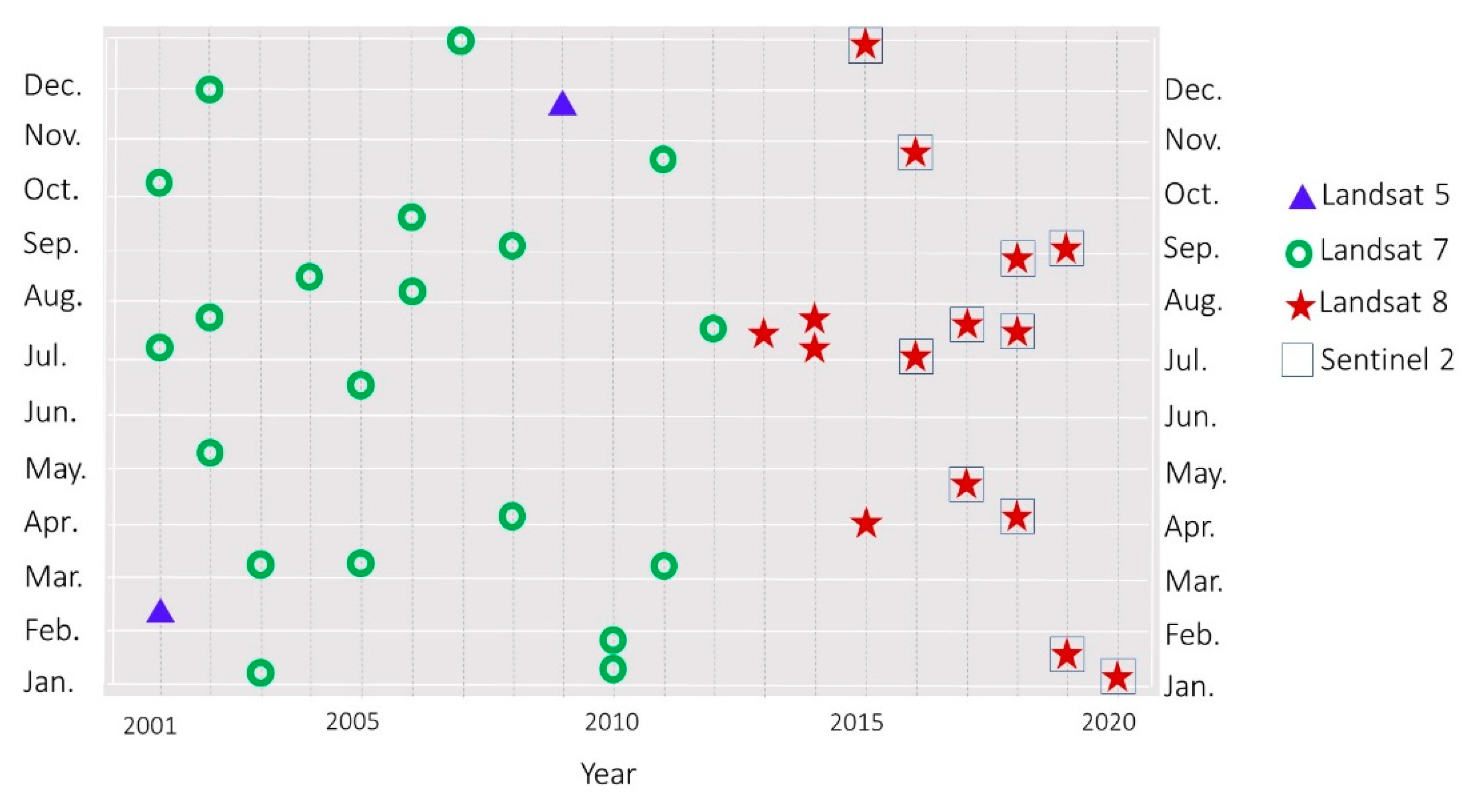

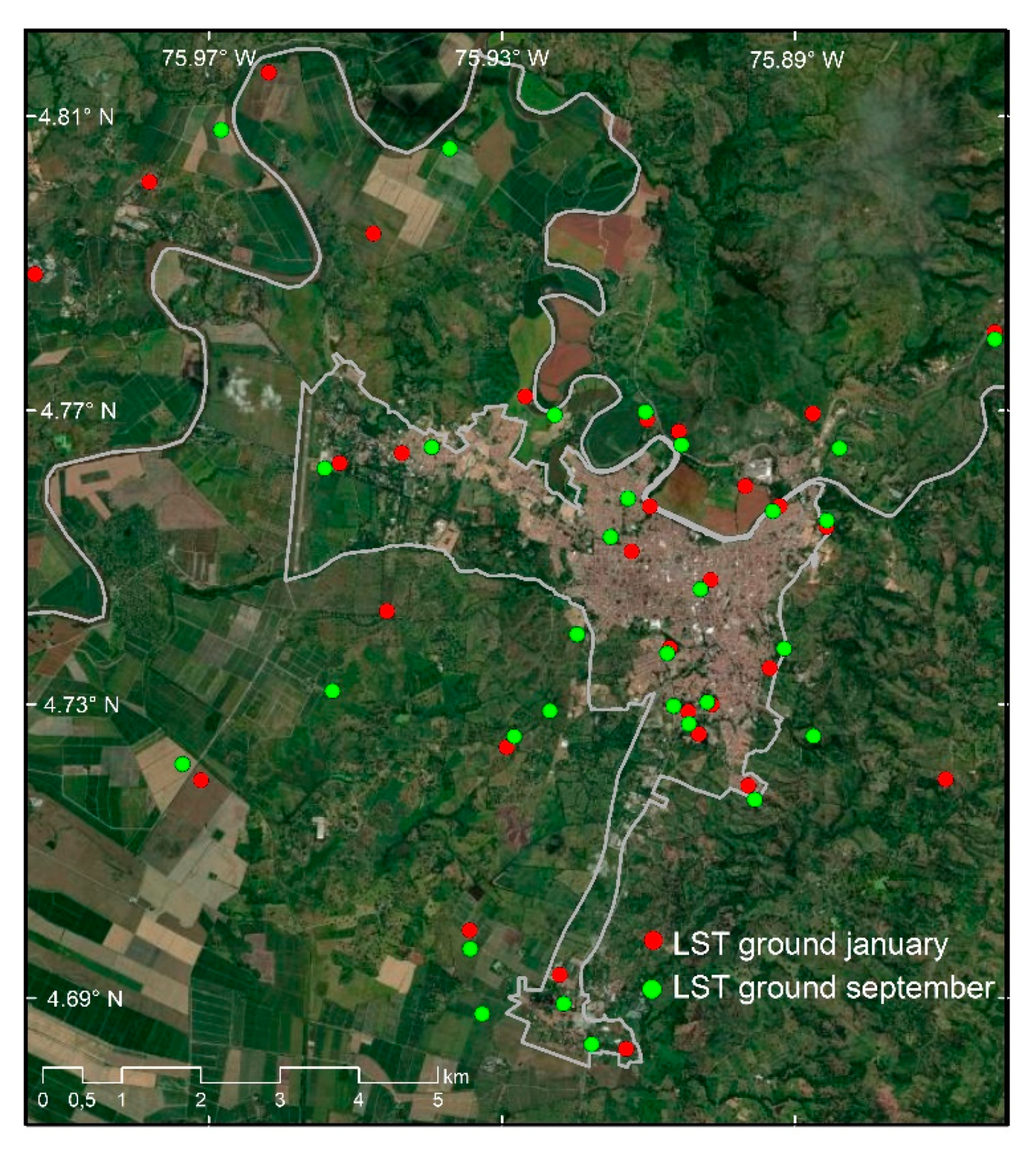
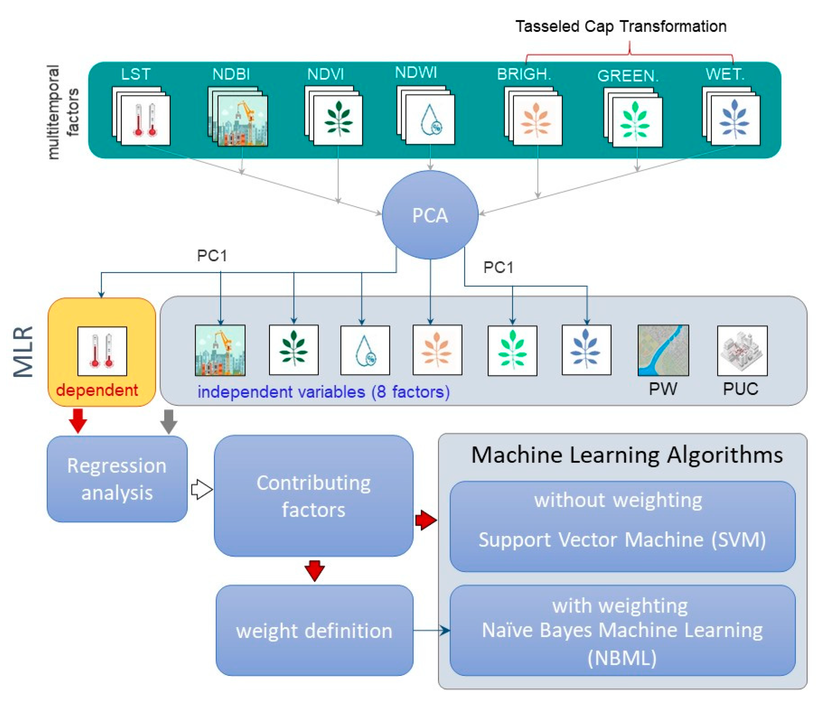
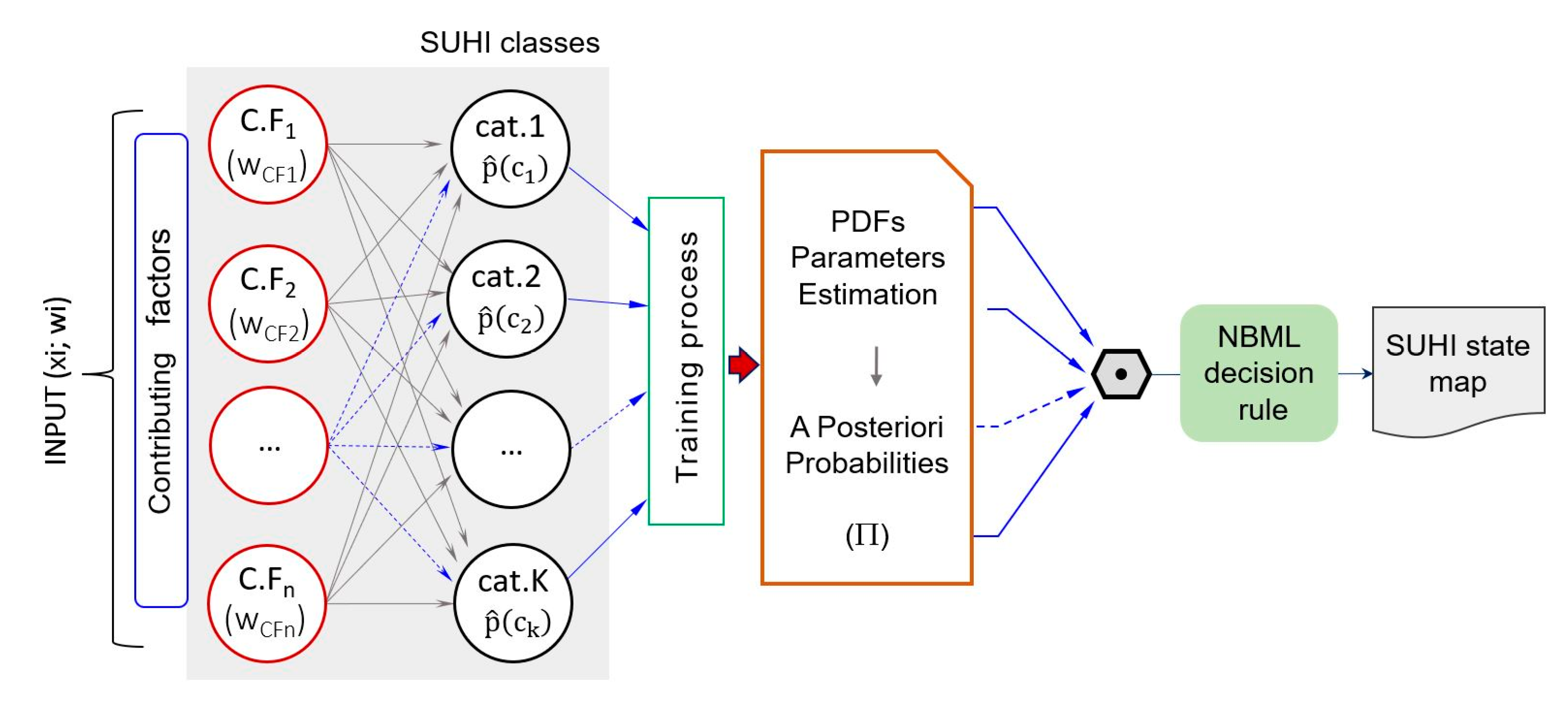
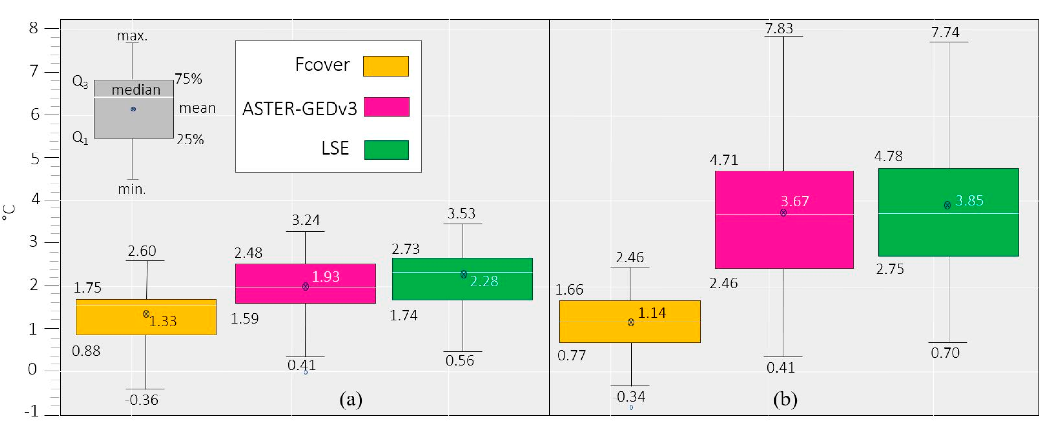
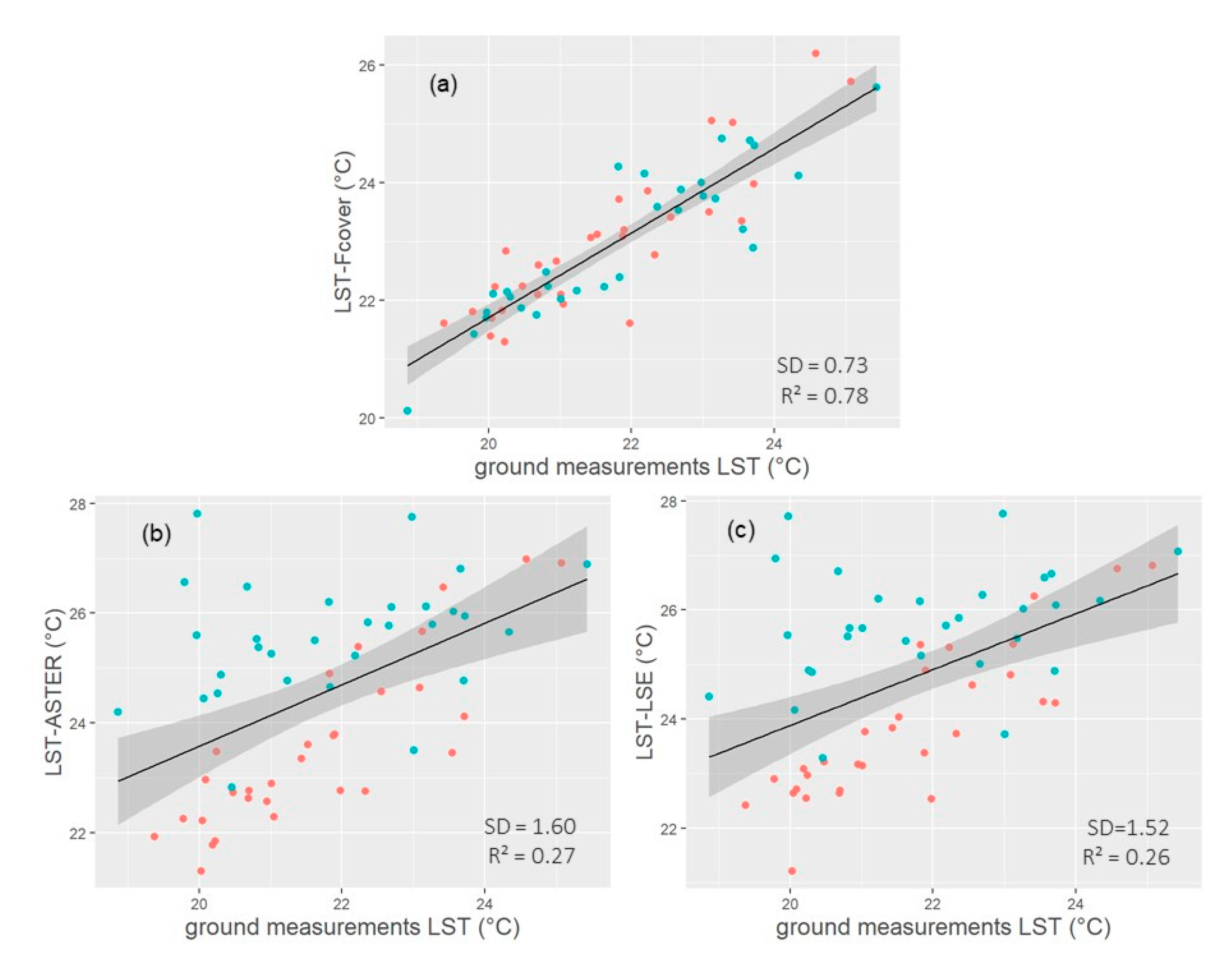
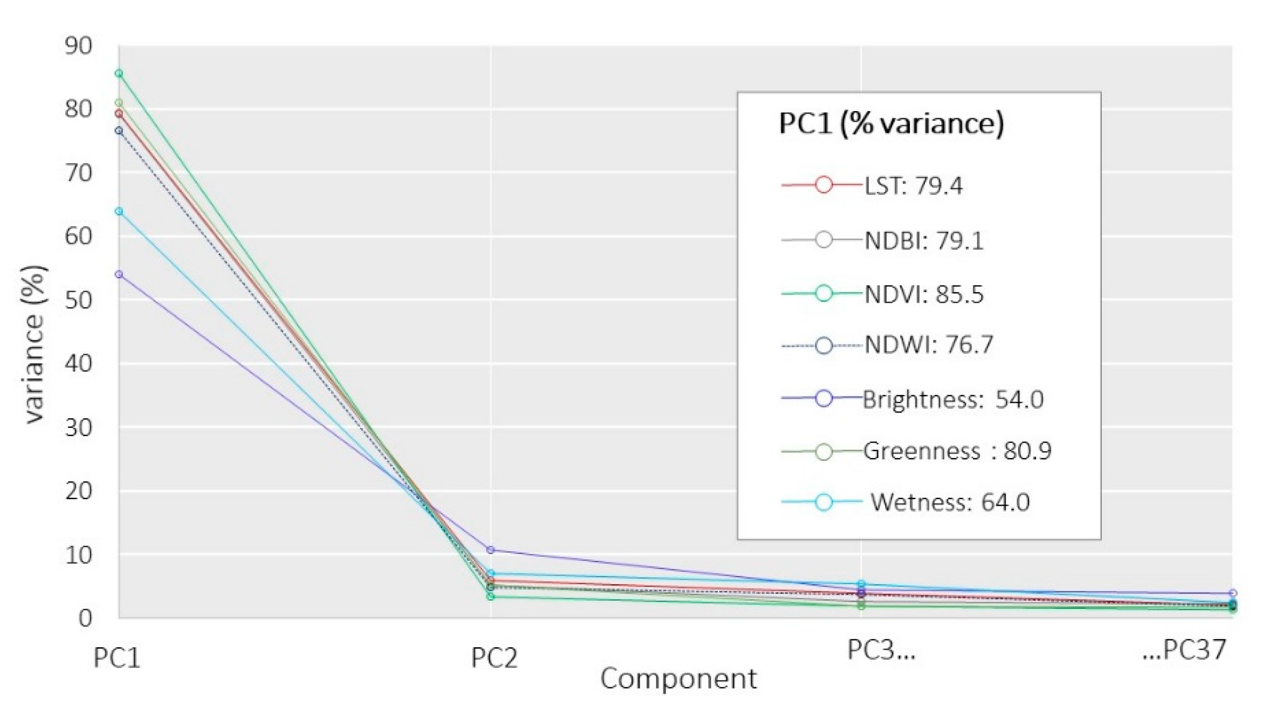
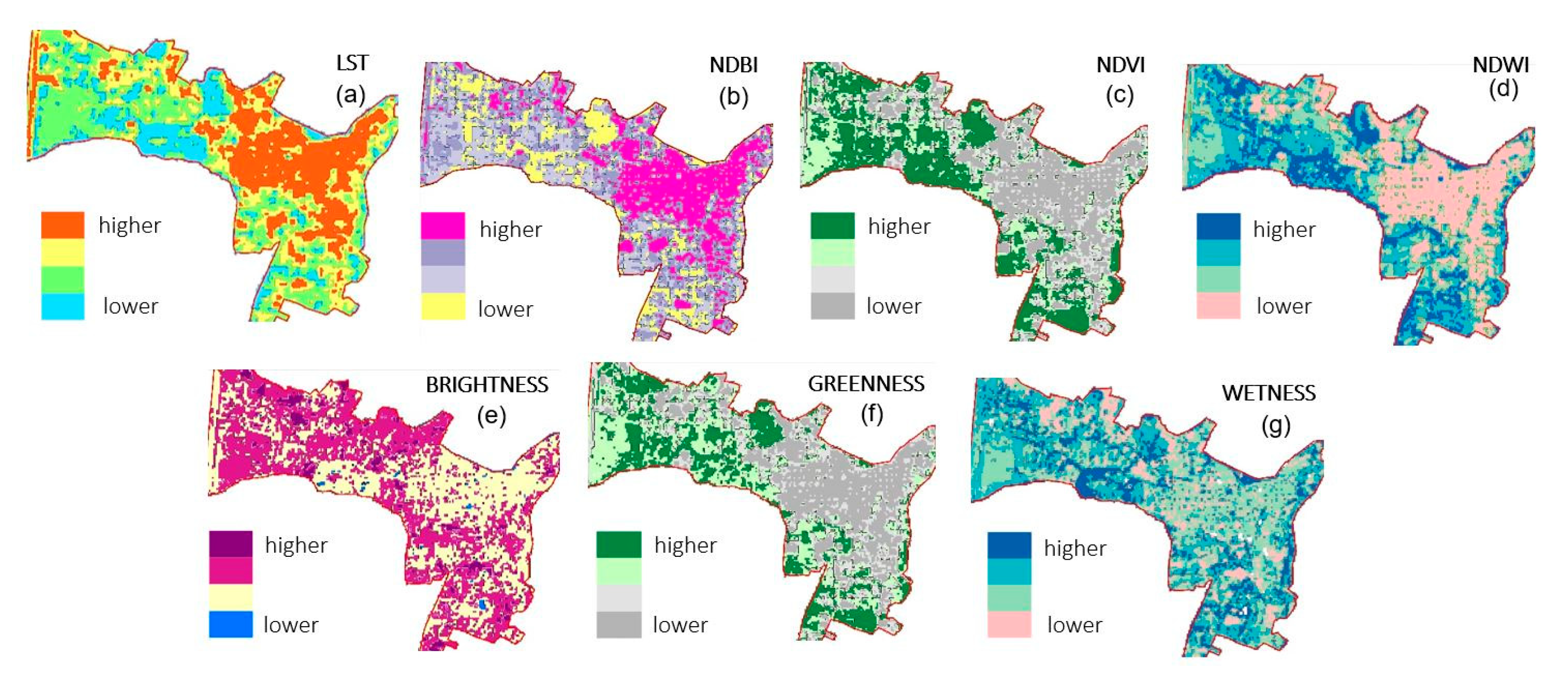
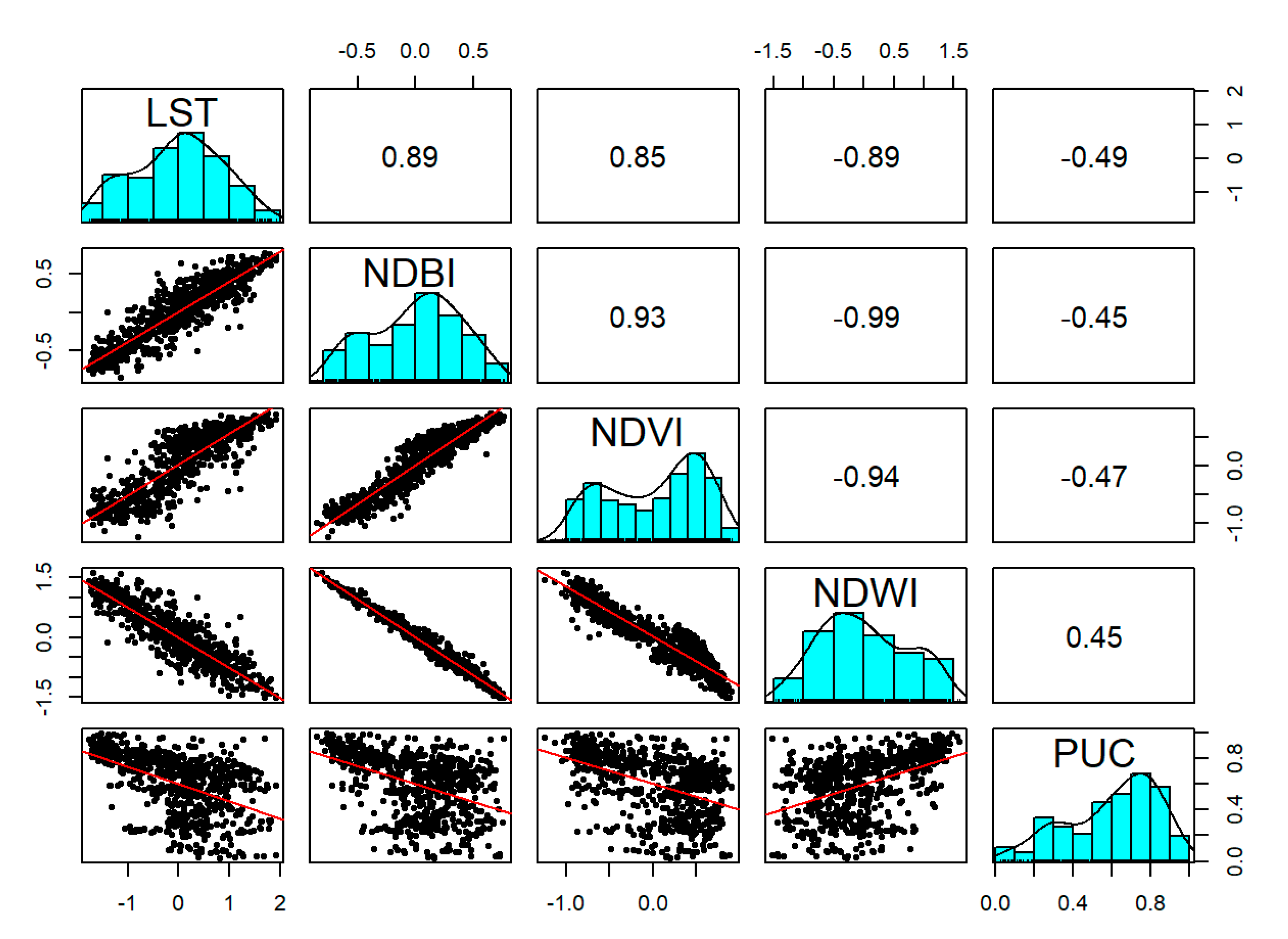
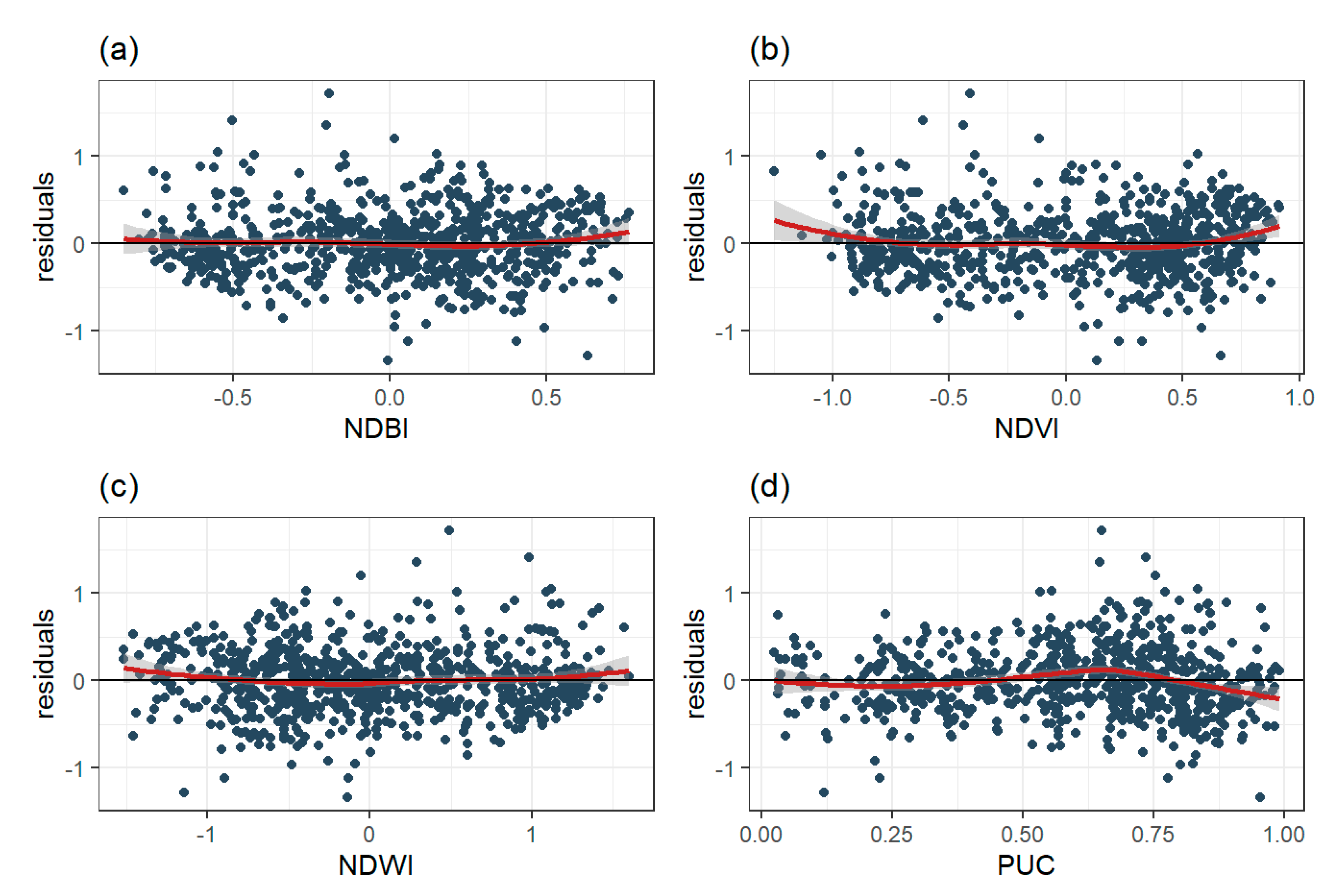
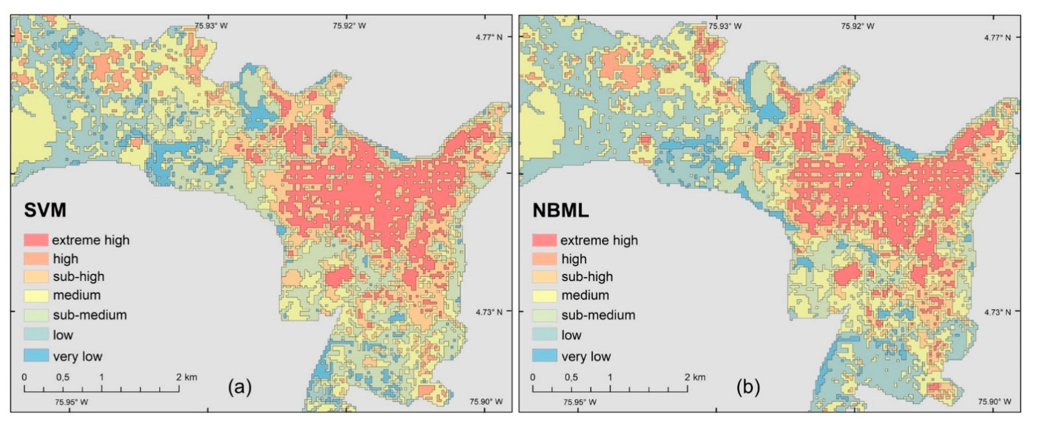
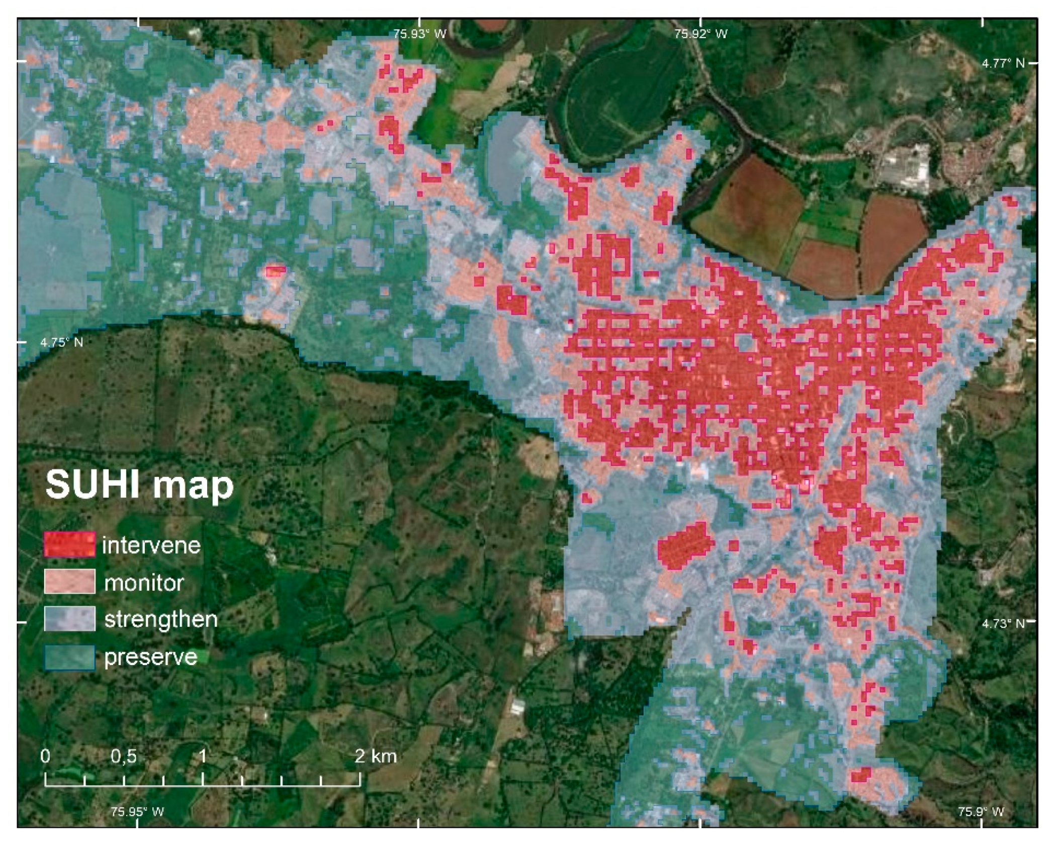
Publisher’s Note: MDPI stays neutral with regard to jurisdictional claims in published maps and institutional affiliations. |
© 2021 by the authors. Licensee MDPI, Basel, Switzerland. This article is an open access article distributed under the terms and conditions of the Creative Commons Attribution (CC BY) license (https://creativecommons.org/licenses/by/4.0/).