
Optimal Estimate of Global Biome—Specific Parameter Settings to Reconstruct NDVI Time Series with the Harmonic ANalysis of Time Series (HANTS) Method


Abstract
:
1. Introduction
- (1)
- Time window applied in compositing the input data. Most freely available NDVI data apply a 10- or 16- or 30-day time window in compositing daily observations by applying maximum value composition (MVC) [37,38,39]. This procedure was believed to be sufficient to eliminate most cloudy observations [11,15]. Most applications were based on such composite data products [16,18,34], although, to our knowledge, no study evaluated the performance of HANTS in processing raw daily NDVI data or products with different composition time windows.
- (2)
- Quality control (QC) information. Pixel-based QC information, which indicates the retrieving reliability (e.g., good, marginal, snow/ice or cloudy), is an indispensable attribute of quantitative remote sensing data products [40]. Previous studies suggested this information could help to exclude low quality observations and improve reconstruction performance [20,37]. The accuracy of QC information, however, may also degrade its reliability [10,12], and the degree to which the QC information may impact the global reconstruction performance of HANTS needs to be investigated.
- (3)
- Actual acquisition date of each observation. For each pixel and time window the MVC procedure selects the maximum NDVI value but does not retain the actual date of acquisition [15,41]. This implies that, e.g., in a 7-day composite, there might be a difference in acquisition time of up to 14 days between the NDVI observations retained in adjacent pixels. This inconsistency can be mitigated by assigning an approximate time stamp, e.g., start, middle or end of the time window, to each selected maximum NDVI observation. However, this solution may still yield large differences between this approximate time stamp and the actual date of acquisition for the retained maximum NDVI value. When applying longer time windows, e.g., 30 days, or when observing critical or shorter phenological stages, the vegetation signal can change significantly during the time window [41,42]. It still needs to be evaluated, therefore, whether the global reconstruction performance might be improved by applying the actual date acquisition of each retained NDVI observation in the reconstruction of the time series.
2. Materials and Methods
2.1. Materials
2.2. Methods
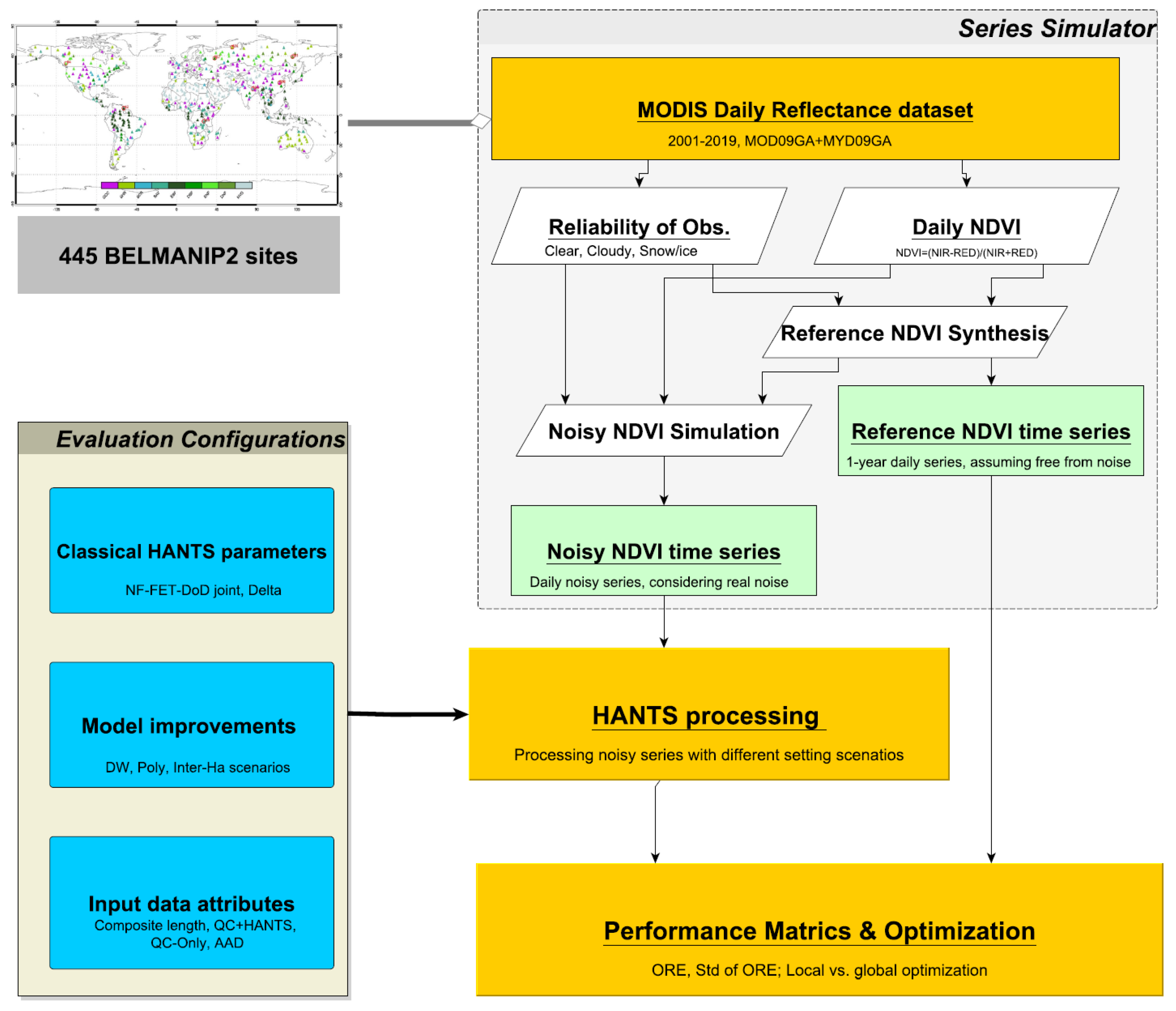
2.2.1. Overview of the Evaluation and Optimization Procedures
2.2.2. Simulation of Reference and Noisy NDVI Time Series
2.2.3. Configurations for Evaluation and Optimization
- (1)
- Configurations of classical HANTS parametersThe performance of HANTS is mainly controlled by multiple critical internal parameters. Except the length of the base period (BP), HiLO flag, and valid range (VR) that can be easily determined based on the physical meaning of the input signal, the other four parameters, i.e., NF, FET, DoD, and Delta, must be selected within a range of possible values by users and the selection procedure needs to be evaluated systematically. A set of configurations needs to be evaluated in order to understand better the impact of each parameter on the model in global NDVI reconstruction and can be briefly described as follows:
- (a)
- Length of base period (BP): This parameter corresponds to the period of the dominant component of the signal to be reconstructed, while the periods of all other harmonics are derived from the base period (see the description of NF below). Remote sensing-based NDVI data are provided at a daily to monthly sampling interval, with the signal dominated by the seasonal and yearly variations in vegetation greenness. Thus, the BP is normally set to 12-month (i.e., one year or 365 days).
- (b)
- Number of frequencies (NF): This parameter determines the total number of harmonics (excluding the zero-frequency component) to be used in the time series modeling and reconstruction. The period of the i-th harmonic is given by P(i) = BP/i (i = 1, 2, …, NF). In turn, the frequency is the reciprocal of P(i). Since atmospheric contamination mainly introduces high frequency noise, a few low frequency components (i.e., NF < 4) were used in previous studies (e.g., [18,30,35]). In this study, NF in the range from 2 (12-month and 6-month components) to 6 was applied, i.e., 2 months was the shortest period/highest frequency component, in the global evaluation of time series reconstruction by HANTS.
- (c)
- Fitting error tolerance (FET): The acceptable maximum deviation between raw observations and the result of the reconstruction. In the case of NDVI(t), at each iteration, a negative deviation from the modeled time series larger than FET will be excluded from further iterative processing. The iteration is terminated when all deviations between the remaining valid observations and the fitted model are smaller than the pre-defined FET value. A small FET may erroneously remove some valid observations as outliers while some real outliers cannot be correctly identified with a too large FET. FET is frequently set between 0.05 and 0.1 in the reconstruction of NDVI time series by HANTS [16,18,44,45]. In this study, a FET range from 0.01 to 0.12 with a 0.01 step was applied.
- (d)
- Degree of over-determinedness (DoD): A Fourier series including the harmonic components determined by BP and NF is used to model the time series of observations. The coefficients of the modeled series are obtained by solving a linear system of equations, which requires at least 2NF + 1 independent observation, since amplitude and phase value need to be determined for each harmonic component of the series. The observations are inherently accompanied with errors, solutions of the system of equations by using > 2NF + 1 observations may improve the accuracy of estimated amplitude and phase. Such an overdetermined system of equations is best solved using least square method, where more observations give a smaller error of estimate. HANTS is designed to identify and remove outliers iteratively. The DoD is defined as the minimum number of required additional observations, i.e., the minimum difference between the remaining valid observation size and 2NF + 1 [35]. In other words, if the total input observation size is N0, then the removed outliers should not exceed (N0 − (DoD + 2NF + 1)). Therefore, the DoD can be set between 0 and (N0 − (2NF + 1)) and it is a second termination criterion of iterations beside FET. A too large DoD tends, however, to prevent the iteration procedure from detecting possible outliers [16]. The minimum number of valid observations needed to solve a system of equations is 13 when NF = 6. So, the maximum possible DoD for 16-day composited yearly NDVI (N0 = 23) is 10. In this study, we varied DoD between 0 and 12 in steps of 1 to analyze the impact of DoD on model performance.
- (e)
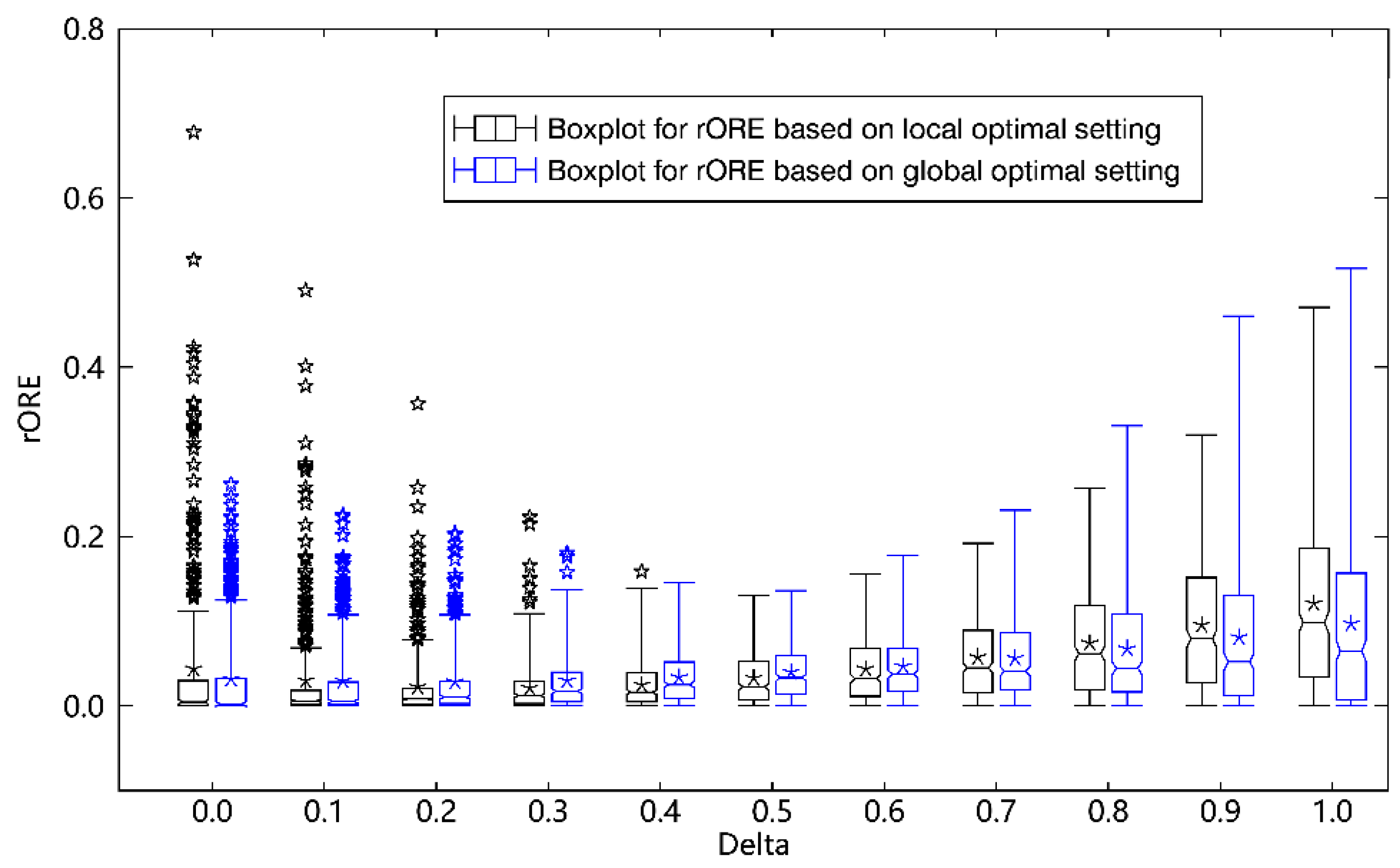
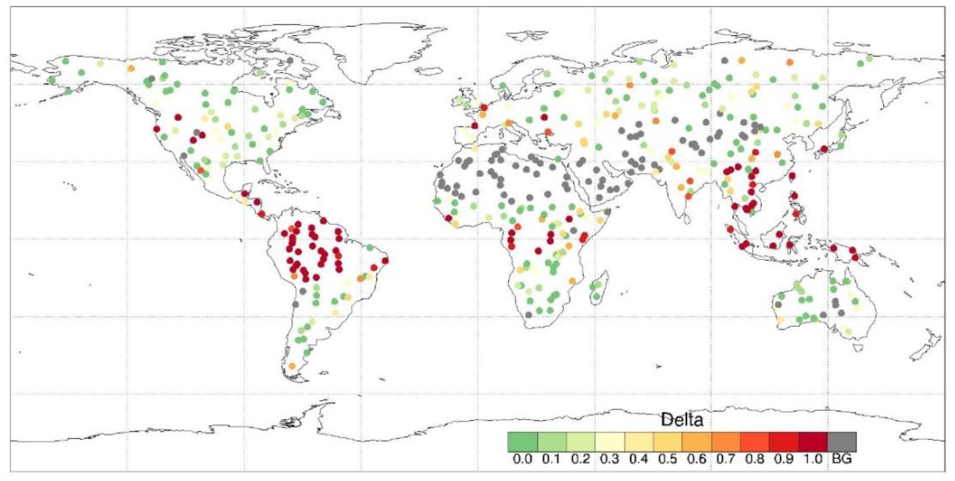
- Delta (regularization factor): Although the solution is obtained by solving an overdetermined linear system of equations in HANTS, the solutions may be non-unique because of possible singular matrixes, i.e., ill-conditioned systems. These non-unique solutions may yield large fluctuations in the fitted results, especially in subsequent iterations. The ridge regression method was applied to solve the linear system in the classical HANTS and a regularization factor (i.e., Delta) was used to damp the randomness of the solutions [20]. The Delta is generally set as a small positive value (e.g., 0.1). The impact on model performance was evaluated by varying Delta between 0 and 1 in step of 0.1.
- (f)
- HiLo flag: This parameter indicates whether outliers are expected either above or below the fitted model, which depends on the nature of observations [16]. For instance, cloud covered or contaminated targets yield lower NDVI values compared to clear-sky conditions, thus outliers are below the fitted model and are rejected (i.e., HiLo = “Low”). Given the type of observations, HiLo parameter is unambiguously defined and there is no need to evaluate the impact on HANTS performance.
- (g)
- Valid range (VR): The valid range of input signals is determined by the nature of the observations and is defined for each data product [16]. For instance, the land surface NDVI generally ranges between 0 (or −0.2 if including water or snow) and 1.0. Observations outside this range can be rejected as outliers directly.
In summary, the NF, FET, DoD, and Delta are the four most critical parameters of classical HANTS controlling the reconstruction performance. The NF, FET, and DoD jointly determine profile fitting and outlier detection of the model, and thus their settings are evaluated jointly. Here the “joint” evaluation means calculating performance metrics over all sites under each possible combination of NF, FET, and DoD settings. For each site, there will be 5 (NF settings) × 12 (FET settings) × 13 (DoD settings) = 780 combinations. Based on the joint evaluation result, the Delta scenarios are further evaluated, after which the optimized parameter settings for global reconstruction using classical HANTS can be derived. - (2)
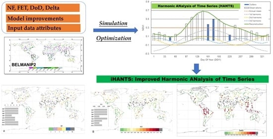
- Model improvementsIn addition to the procedure to optimize parameter settings of the classical HANTS, several ways to improve global reconstruction performance by adapting the design of HANTS were proposed.Specifically, the proposed improvements and the procedures to evaluate them are described below:
- (a)
- Dynamic update of weights. Initially, all input observations are assigned a weight = 1 by HANTS. The algorithm was originally designed to apply varying weights, but it was first implemented with binary weights, i.e., = 1 for valid observations and = 0 for outliers. As explained above, at each iteration, any observation negatively deviating from the current Fourier series by more than the FET are assigned a weight = 0 and excluded in further iterations. The FET setting is set on the basis of user experience and erroneous detection of outlier is unavoidable. The dynamic update of weights was proposed to improve the performance. In practice, the weight of the i-th observation is updated at each k-th iteration taking into account the deviation from the current Fourier series as:where yrk is the vector of estimates by the Fourier series at the k-th iteration. In this case, if the k-th estimates are larger than estimates in the previous iteration, weights are increased. This leads to the estimates in later iterations to approach the upper envelope of NDVI time-series.
- (b)
- Polynomial or inter-annual harmonic components: If HANTS is applied to annual NDVI time series, the estimated Fourier components can only explain variations over periods shorter than a year while real signals may contain trends or inter-annual variations [12]. Earlier studies on Fourier analysis of NDVI time series were focused on investigate inter-annual variation of vegetation regulated by climate using multi-annual data records [30,46,47,48]. Multi-annual components in the Fourier series or alternatively 3-order polynomial components can be used to capture inter-annual variability.
- (3)
- Impact of input data attributesThe impact on reconstruction performance of key—characteristics of input data was evaluated, specifically the time window applied in the compositing, QC information, and the actual date of acquisition of the observation retained in the temporal composite for each time window and each pixel:
- (a)
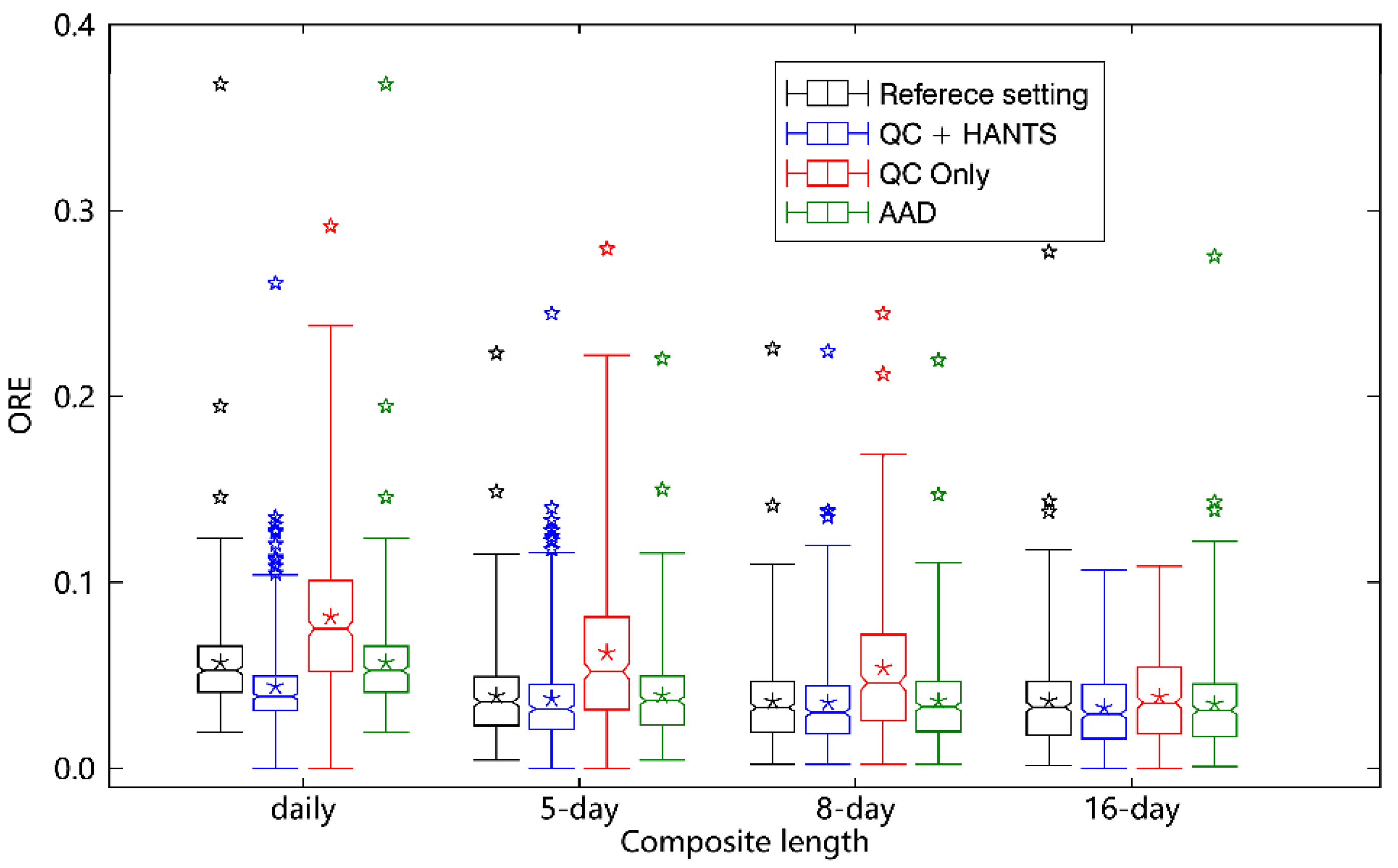
- Composite time window. MVC-s were generated applying a time window of 1, 5, 8, and 16 days and used to simulate daily noisy series for each site. The overall reconstruction error (ORE) was calculated to evaluate the impact of the MVC time window on reconstruction performance.
- (b)
- QC-based weighting. The QC flag of each observation was used in the reconstruction. The weights are set initially as 0 or 1 for low quality observations (QC = 0) or high-quality observations (QC = 1) respectively.
- (c)
- Actual date of acquisition. The actual date of acquisition of the observation retained in the temporal composite for each time window and each pixel was used in the reconstruction instead of the average or central date within each time window.
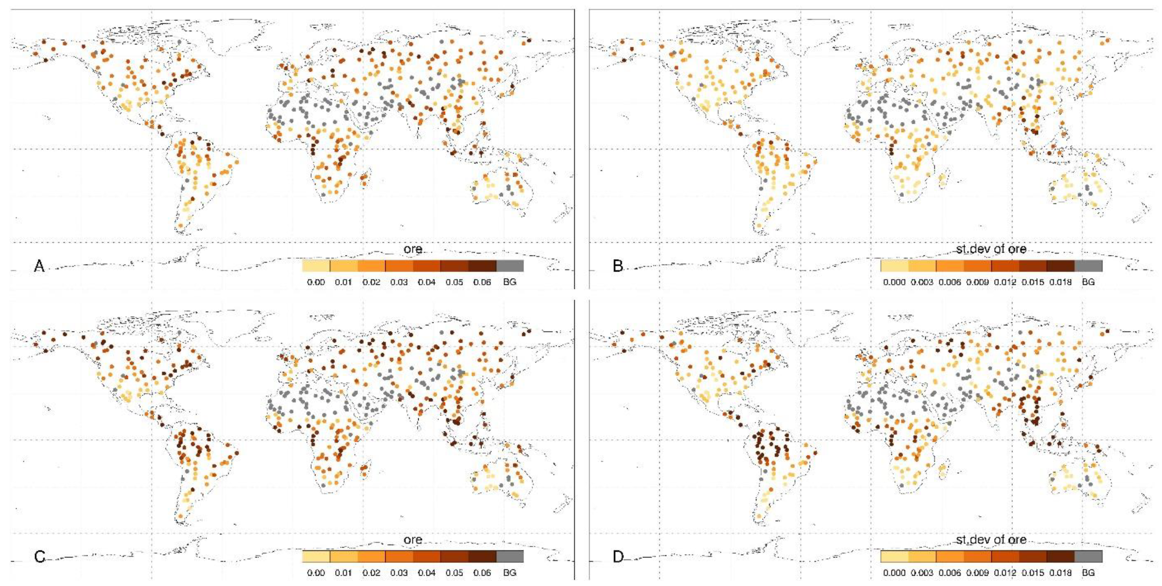
2.2.4. Performance Metrics
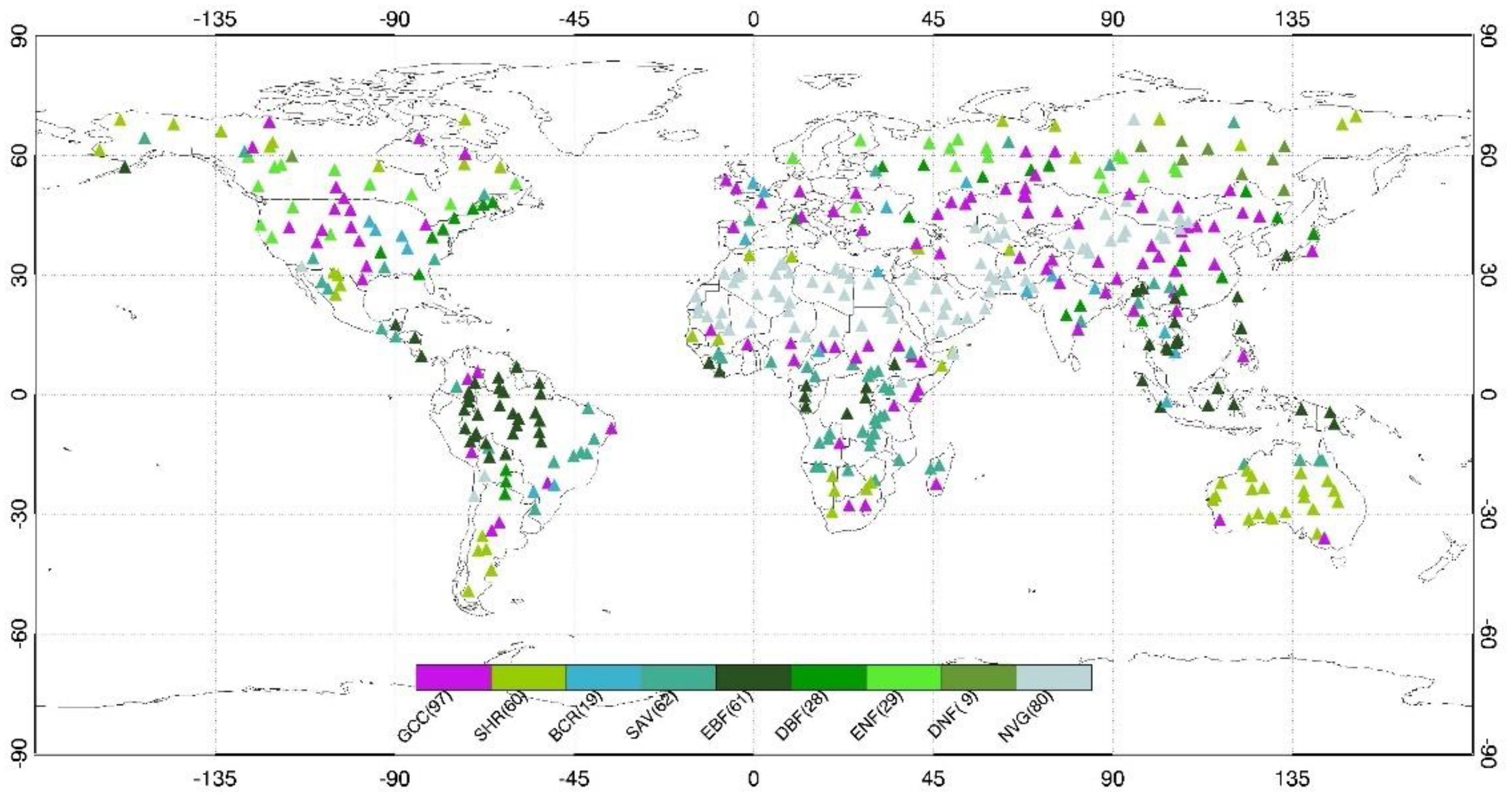
- = 1, 2, …, 445 sites;
- = 1, 2, …, 100 noisy series;
- is the k-th estimate of j-th reconstructed noisy NDVI series for the i-th site;
- is the k-th estimate of simulated reference NDVI series for i-th site;
- (=365) is the number of samples in each reconstructed time series.
3. Results
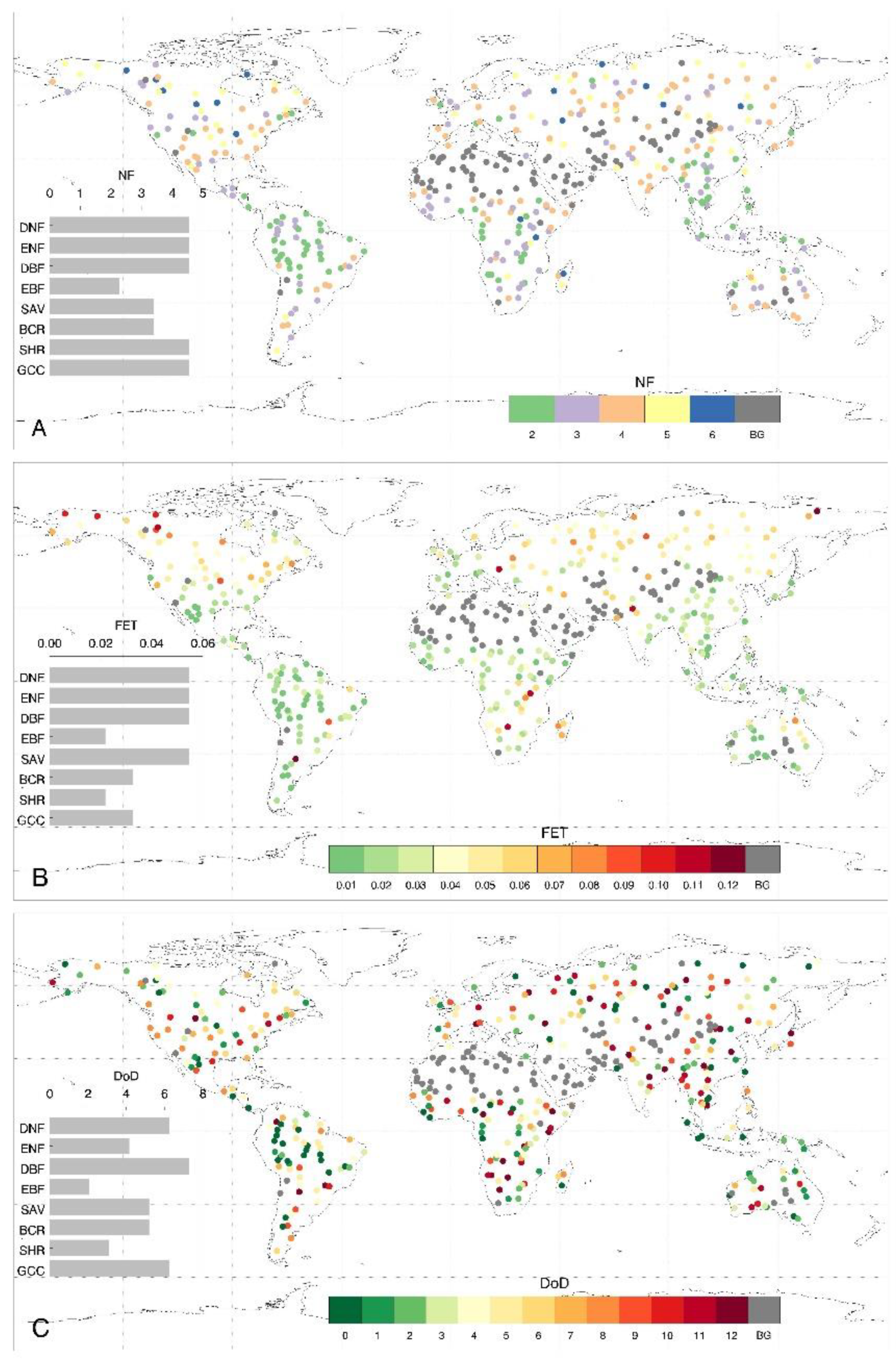
3.1. Optimization of Parameter Setting
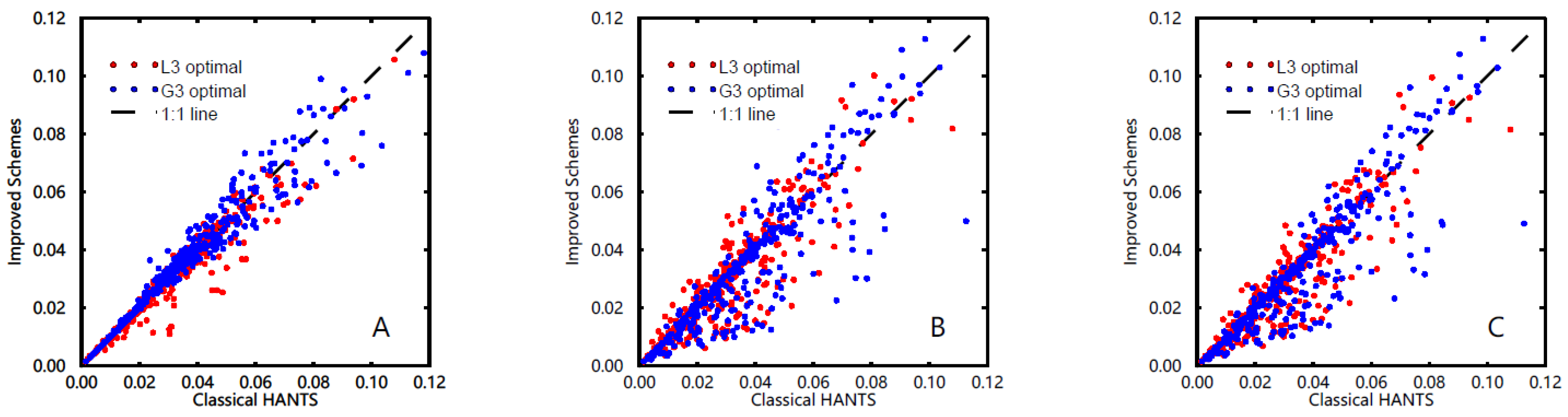
3.2. Impact of Proposed Improvements
3.3. Impact of Input Data Attributes
4. Discussion
4.1. The Improved Harmonic ANalysis of Time Series (iHANTS)
- (1)
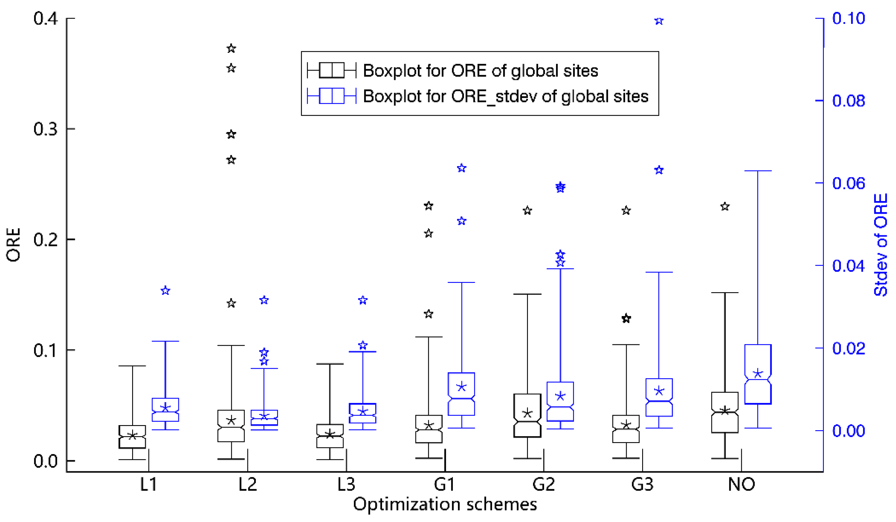
- The critical internal parameters, i.e., NF, FET, DoD and Delta can be set on the basis of either a “local” or “global” ranking for global reconstruction. For regional applications, users can refer to Figure 3 and Figure 6 for best local settings. The best global settings, based on the trade-off between ORE and Std-ORE, are: NF = 4, FET = 0.05, DOD = 5, and Delta = 0.5, which is the default setting scheme used by [18] to evaluate the performance of global NDVI reconstruction.
- (2)
- Reconstruction performance can be significantly improved in specific regions of the Earth by using dynamic weighting instead of the classical rigid weighting scheme and by adding 3-order polynomial or inter-annual harmonic components to account for inter-annual variability. Dynamic weighting and 3-order polynomial components require a revised implementation of HANTS.
- (3)
- Global reconstruction performance can be improved by using QC information of the dataset to set initial weight and applying the actual date of acquisition for each input observation. Most freely accessible implementations of HANTS do not support custom setting of initial weights and input timestamps. Thus, a revised implementation of the model is needed again.
4.2. Applying Optimaized HANTS to Other Terrestrial Remote Sensing Variables
4.3. Other Application Topics for the HANTS
5. Conclusions
Supplementary Materials
Author Contributions
Funding
Institutional Review Board Statement
Informed Consent Statement
Data Availability Statement
Conflicts of Interest
References
- Zeng, L.; Wardlow, B.D.; Xiang, D.; Hu, S.; Li, D. A review of vegetation phenological metrics extraction using time-series, multispectral satellite data. Remote Sens. Environ. 2020, 237, 111511. [Google Scholar] [CrossRef]
- Yao, X.; Li, G.; Xia, J.; Ben, J.; Cao, Q.; Zhao, L.; Ma, Y.; Zhang, L.; Zhu, D. Enabling the big earth observation data via cloud computing and DGGS: Opportunities and challenges. Remote Sens. 2020, 12, 62. [Google Scholar] [CrossRef] [Green Version]
- Xue, J.; Su, B. Significant remote sensing vegetation indices: A review of developments and applications. J. Sens. 2017, 2017, 1–17. [Google Scholar] [CrossRef] [Green Version]
- Huang, S.; Tang, L.; Hupy, J.P.; Wang, Y.; Shao, G. A commentary review on the use of normalized difference vegetation index (NDVI) in the era of popular remote sensing. J. For. Res. 2021, 32, 1–6. [Google Scholar] [CrossRef]
- Sudmanns, M.; Tiede, D.; Lang, S.; Bergstedt, H.; Trost, G.; Augustin, H.; Baraldi, A.; Blaschke, T. Big earth data: Disruptive changes in earth observation data management and analysis? Int. J. Digit. Earth 2020, 13, 832–850. [Google Scholar] [CrossRef]
- Guo, H.; Nativi, S.; Liang, D.; Craglia, M.; Wang, L.; Schade, S.; Corban, C.; He, G.; Pesaresi, M.; Li, J.; et al. Big earth data science: An information framework for a sustainable planet. Int. J. Digit. Earth 2020, 13, 743–767. [Google Scholar] [CrossRef] [Green Version]
- Zhu, Z.; Wulder, M.A.; Roy, D.P.; Woodcock, C.E.; Hansen, M.C.; Radeloff, V.C.; Healey, S.P.; Schaaf, C.; Hostert, P.; Strobl, P.; et al. Benefits of the free and open landsat data policy. Remote Sens. Environ. 2019, 224, 382–385. [Google Scholar] [CrossRef]
- Wulder, M.A.; Loveland, T.R.; Roy, D.P.; Crawford, C.J.; Masek, J.G.; Woodcock, C.E.; Allen, R.G.; Anderson, M.C.; Belward, A.S.; Cohen, W.B.; et al. Current status of landsat program, science, and applications. Remote Sens. Environ. 2019, 225, 127–147. [Google Scholar] [CrossRef]
- Fensholt, R.; Sandholt, I.; Stisen, S.; Tucker, C. Analysing NDVI for the African continent using the geostationary meteosat second generation seviri sensor. Remote Sens. Environ. 2006, 101, 212–229. [Google Scholar] [CrossRef]
- Julien, Y.; Sobrino, J.A. Optimizing and comparing gap-filling techniques using simulated NDVI time series from remotely sensed global data. Int. J. Appl. Earth Obs. Geoinf. 2019, 76, 93–111. [Google Scholar] [CrossRef]
- Holben, B.N. Characteristics of maximum-value composite images from temporal avhrr data. Int. J. Remote Sens. 1986, 7, 1417–1434. [Google Scholar] [CrossRef]
- Zhou, J.; Jia, L.; Menenti, M.; Gorte, B. On the performance of remote sensing time series reconstruction methods–A spatial comparison. Remote Sens. Environ. 2016, 187, 367–384. [Google Scholar] [CrossRef]
- Sarmah, S.; Jia, G.; Zhang, A.; Singha, M. Assessing seasonal trends and variability of vegetation growth from NDVI3g, MODIS NDVI and EVI over South Asia. Remote Sens. Lett. 2018, 9, 1195–1204. [Google Scholar] [CrossRef]
- Ql, J.; Kerr, Y. On current compositing algorithms. Remote Sens. Rev. 1997, 15, 235–256. [Google Scholar] [CrossRef]
- van Leeuwen, W.J.D.; Huete, A.R.; Laing, T.W. MODIS vegetation index compositing approach: A prototype with AVHRR data. Remote Sens. Environ. 1999, 69, 264–280. [Google Scholar] [CrossRef]
- Roerink, G.J.; Menenti, M.; Verhoef, W. Reconstructing cloudfree NDVI composites using fourier analysis of time series. Int. J. Remote Sens. 2000, 21, 1911–1917. [Google Scholar] [CrossRef]
- Nagai, S.; Saitoh, T.M.; Suzuki, R.; Nasahara, K.N.; Lee, W.-K.; Son, Y.; Muraoka, H. The necessity and availability of noise-free daily satellite-observed NDVI during rapid phenological changes in terrestrial ecosystems in East Asia. For. Sci. Technol. 2011, 7, 174–183. [Google Scholar] [CrossRef]
- Zhou, J.; Jia, L.; Menenti, M. Reconstruction of global MODIS NDVI time series: Performance of harmonic analysis of time series (HANTS). Remote Sens. Environ. 2015, 163, 217–228. [Google Scholar] [CrossRef]
- Jonsson, P.; Eklundh, L. Seasonality extraction by function fitting to time-series of satellite sensor data. IEEE T Geosci. Remote 2002, 40, 1824–1832. [Google Scholar] [CrossRef]
- Chen, J.; Jönsson, P.; Tamura, M.; Gu, Z.; Matsushita, B.; Eklundh, L. A Simple method for reconstructing a high-quality NDVI time-series data set based on the savitzky–golay filter. Remote Sens. Environ. 2004, 91, 332–344. [Google Scholar] [CrossRef]
- Julien, Y.; Sobrino, J.A. Comparison of cloud-reconstruction methods for time series of composite NDVI data. Remote Sens. Environ. 2010, 114, 618–625. [Google Scholar] [CrossRef]
- Atzberger, C.; Eilers, P.H.C. A time series for monitoring vegetation activity and phenology at 10-daily time steps covering large parts of South America. Int. J. Digit. Earth 2011, 4, 365–386. [Google Scholar] [CrossRef]
- Vuolo, F.; Ng, W.-T.; Atzberger, C. Smoothing and gap-filling of high resolution multi-spectral time series: Example of landsat data. Int. J. Appl. Earth Obs. Geoinf. 2017, 57, 202–213. [Google Scholar] [CrossRef]
- Menenti, M.; Malamiri, H.R.G.; Shang, H.; Alfieri, S.M.; Maffei, C.; Jia, L. Observing the response of terrestrial vegetation to climate variability across a range of time scales by time series analysis of land surface temperature. In Multitemporal Remote Sensing: Methods and Applications; Ban, Y., Ed.; Springer International Publishing: Berlin/Heidelberg, Germany, 2016; pp. 277–315. ISBN 978-3-319-47037-5. [Google Scholar]
- Geng, L.; Ma, M.; Wang, X.; Yu, W.; Jia, S.; Wang, H. Comparison of eight techniques for reconstructing multi-satellite sensor time-series NDVI data sets in the Heihe River Basin, China. Remote Sens. 2014, 6, 2024–2049. [Google Scholar] [CrossRef] [Green Version]
- Shen, H.; Li, X.; Cheng, Q.; Zeng, C.; Yang, G.; Li, H.; Zhang, L. Missing information reconstruction of remote sensing data: A technical review. IEEE Geosci. Remote Sens. Mag. 2015, 3, 61–85. [Google Scholar] [CrossRef]
- Zhou, J.; Jia, L.; van Hoek, M.; Menenti, M.; Lu, J.; Hu, G. An optimization of parameter settings in HANTS for global NDVI time series reconstruction. In Proceedings of the 2016 IEEE International Geoscience and Remote Sensing Symposium (IGARSS), Beijing, China, 10–15 July 2016; pp. 3422–3425. [Google Scholar]
- Julien, Y.; Sobrino, J.A. TISSBERT: A benchmark for the validation and comparison of ndvi time series reconstruction methods. Rev. De Teledetección 2018, 51, 19–31. [Google Scholar] [CrossRef]
- Zhu, Z.; Woodcock, C.E.; Holden, C.; Yang, Z. Generating synthetic landsat images based on all available landsat data: Predicting landsat surface reflectance at any given time. Remote Sens. Environ. 2015, 162, 67–83. [Google Scholar] [CrossRef]
- Menenti, M.; Azzali, S.; Verhoef, W.; van Swol, R. Mapping agroecological zones and time lag in vegetation growth by means of fourier analysis of time series of NDVI images. Adv. Space Res. 1993, 13, 233–237. [Google Scholar] [CrossRef]
- Sellers, P.J.; Tucker, C.J.; Collatz, G.J.; Los, S.O.; Justice, C.O.; Dazlich, D.A.; Randall, D.A. A Global 1-degrees-by-1-degrees Ndvi data set for climate studies. 2. the generation of global fields of terrestrial biophysical parameters from the Ndvi. Int. J. Remote Sens. 1994, 15, 3519–3545. [Google Scholar] [CrossRef]
- Jakubauskas, M.E.; Legates, D.R.; Kastens, J.H. Harmonic analysis of time-series AVHRR NDVI data. Photogramm. Eng. Remote Sens. 2001, 67, 461–470. [Google Scholar]
- Xie, F.; Fan, H. Deriving drought indices from MODIS vegetation indices (NDVI/EVI) and land surface temperature (LST): Is data reconstruction necessary? Int. J. Appl. Earth Obs. Geoinf. 2021, 101, 102352. [Google Scholar] [CrossRef]
- Menenti, M.; Jia, L.; Roerink, G.J.; Gonzalez-Loyarte, M.; Leguizamon, S.; Verhoef, W. Analysis of vegetation response to climate variability using extended time series of multispectral satellite images. In Remote Sensing Optical Observations of Vegetation Properties; Maselli, F., Massimo, M., Brivio, P.A., Eds.; Research Signpost: Kerala, India, 2010; pp. 131–163. ISBN 978-81-308-0421-7. [Google Scholar]
- Verhoef, W. Application of Harmonic Analysis of NDVI Time Series (HANTS); Fourier Analysis of Temporal NDVI in the Southern African and American Continents; DLO Winand Staring Centre: Wageningen, The Netherlands, 1996; pp. 19–24. [Google Scholar]
- Gorelick, N.; Hancher, M.; Dixon, M.; Ilyushchenko, S.; Thau, D.; Moore, R. Google earth engine: Planetary-scale geospatial analysis for everyone. Remote Sens. Environ. 2017, 202, 18–27. [Google Scholar] [CrossRef]
- Huete, A.; Didan, K.; Miura, T.; Rodriguez, E.P.; Gao, X.; Ferreira, L.G. Overview of the radiometric and biophysical performance of the MODIS vegetation indices. Remote Sens. Environ. 2002, 83, 195–213. [Google Scholar] [CrossRef]
- Tucker, C.J.; Pinzon, J.E.; Brown, M.E.; Slayback, D.A.; Pak, E.W.; Mahoney, R.; Vermote, E.F.; El Saleous, N. An extended AVHRR 8-Km NDVI dataset compatible with MODIS and SPOT vegetation NDVI data. Int. J. Remote Sens. 2005, 26, 4485–4498. [Google Scholar] [CrossRef]
- Amri, R.; Zribi, M.; Lili-Chabaane, Z.; Duchemin, B.; Gruhier, C.; Chehbouni, A. Analysis of vegetation behavior in a north african semi-arid region, Using SPOT-VEGETATION NDVI data. Remote Sens. 2011, 3, 2568–2590. [Google Scholar] [CrossRef] [Green Version]
- Roy, D.P.; Borak, J.S.; Devadiga, S.; Wolfe, R.E.; Zheng, M.; Descloitres, J. The MODIS land product quality assessment approach. Remote Sens. Environ. 2002, 83, 62–76. [Google Scholar] [CrossRef]
- Testa, S.; Mondino, E.C.B.; Pedroli, C. Correcting MODIS 16-day composite NDVI time-series with actual acquisition dates. Eur. J. Remote Sens. 2014, 47, 285–305. [Google Scholar] [CrossRef]
- Testa, S.; Soudani, K.; Boschetti, L.; Borgogno Mondino, E. MODIS-derived EVI, NDVI and WDRVI time series to estimate phenological metrics in french deciduous forests. Int. J. Appl. Earth Obs. Geoinf. 2018, 64, 132–144. [Google Scholar] [CrossRef]
- Baret, F.; Morissette, J.T.; Fernandes, R.A.; Champeaux, J.L.; Myneni, R.B.; Chen, J.; Plummer, S.; Weiss, M.; Bacour, C.; Garrigues, S.; et al. Evaluation of the representativeness of networks of sites for the global validation and intercomparison of land biophysical products: Proposition of the CEOS-BELMANIP. IEEE T Geosci. Remote 2006, 44, 1794–1803. [Google Scholar] [CrossRef]
- de Jong, R.; de Bruin, S.; de Wit, A.; Schaepman, M.E.; Dent, D.L. Analysis of monotonic greening and browning trends from global NDVI time-series. Remote Sens. Environ. 2011, 115, 692–702. [Google Scholar] [CrossRef] [Green Version]
- Julien, Y.; Sobrino, J.A.; Verhoef, W. Changes in land surface temperatures and NDVI values over Europe between 1982 and 1999. Remote Sens. Environ. 2006, 103, 43–55. [Google Scholar] [CrossRef]
- Azzali, S.; Menenti, M. Mapping vegetation-soil-climate complexes in southern Africa using temporal fourier analysis of NOAA-AVHRR NDVI data. Int. J. Remote Sens. 2000, 21, 973–996. [Google Scholar] [CrossRef]
- Loyarte, M.M.G.; Menenti, M.; Diblasi, A.M. Modelling bioclimate by means of fourier analysis of NOAA-AVHRR NDVI time series in western Argentina. Int. J. Climatol. 2008, 28, 1175–1188. [Google Scholar] [CrossRef]
- Roerink, G.J.; Menenti, M.; Soepboer, W.; Su, Z. Assessment of climate impact on vegetation dynamics by using remote sensing. Phys. Chem. Earth Parts A/B/C 2003, 28, 103–109. [Google Scholar] [CrossRef]
- Lu, X.; Liu, R.; Liu, J.; Liang, S. Removal of noise by wavelet method to generate high quality temporal data of terrestrial MODIS products. Photogramm Eng. Rem S 2007, 73, 1129. [Google Scholar] [CrossRef] [Green Version]
- Jiang, C.; Ryu, Y.; Fang, H.; Myneni, R.; Claverie, M.; Zhu, Z. Inconsistencies of interannual variability and trends in long-term satellite leaf area index products. Glob. Chang. Biol. 2017, 23, 4133–4146. [Google Scholar] [CrossRef] [PubMed]
- Alfieri, S.M.; De Lorenzi, F.; Menenti, M. Mapping air temperature using time series analysis of LST: The SINTESI approach. Nonlin. Process. Geophys. 2013, 20, 513–527. [Google Scholar] [CrossRef] [Green Version]
- Xu, Y.; Shen, Y. Reconstruction of the land surface temperature time series using harmonic analysis. Comput. Geosci. 2013, 61, 126–132. [Google Scholar] [CrossRef]


| Implementation of HANTS Version | Programing Language | Main Features | Author (First Release Year) |
|---|---|---|---|
| HANTS_Fortran_Verhoef [*1] | Fortran | With graphic user interface (GUI); Batch processing in command line | Verhoef (1996) |
| HANTS_IDL_Wit [*2] | IDL/ENVI (2004) | Implemented with IDL/ENVI APIs; Support parallel processing (Make full usage of the multiple processors of CPU) | Wit (2004) |
| TS_HANTS [*3] | IDL | Introduced as an official API in IDL 8.4 in 2014; Only support single series processing | N/A (2014) |
| HANTS_Matlab [*4] | Matlab | Exactly translated from the Fortran version of Verhoef; No tiling scheme, so the PC memory may pose a limitation on the processing | Mohammad Abouali (2011) |
| HANTS_C_Metz [*5] | C | An addon function of GRASS software; Only one function for image set processing | Markus Metz (2013) |
| HANTS_Python_Mattijn [*6] | Python | Demo python implementation of HANTS that can process single series; First publicly available python version. | van Hoek (2015) |
| HANTS_Python_ED [*7] | Python | Complete implementation of HANTS in python support image set processing | Espinoza-Dávalos et al., (2017) |
| HANTS_GEE_Zhou [*8] | Javascript /Python | Implemented on the Google earth engine (GEE) platform; Quick processing because of large volume earth observation dataset and powerful computation capacity provided by GEE | Zhou (2019) |
| HANTS-GeoTS [*9] | R | Full processing flow for remote sensing time series gap-filling considering both pre-processing and reconstruction. | Tecuapetla-Gómez (2020) |
| Parameter Name | Configuration Setting | The Number of Configurations | |
|---|---|---|---|
| Classical model parameter settings | Length of Base Period (BP) | 365 days * | 1 |
| Number of Frequencies (NF) | 2 to 6 in steps of 1 | 6 | |
| Fitting error tolerance (FET) | 0.01 to 0.12 in steps of 0.01 | 12 | |
| Degree of Overdeterminess (DoD) | 0 to 12 in steps of 1 | 13 | |
| Delta | 0 to 1 in steps of 0.1 | 11 | |
| HiLo flag | Low * | 1 | |
| Valid Range (VR) | [0, 1] * | 1 | |
| Proposed Improvements | Dynamic weights (DW) | Non-DW; DW | 2 |
| Polynomial components (PC) | Non-PC; PC | 2 | |
| Interannual Harmonics (Inter-Ha) | Non-Inter-Ha, Inter-Ha | 2 | |
| Data attributes | Compositing lengths (CL) | Daily, 5-day, 8-day, 16-day | 4 |
| Quality Control information (QC) | With-QC, QC-only, Without-QC | 3 | |
| Actual acquisition date (AAD) | With-AAD, Without-AAD | 2 |
Publisher’s Note: MDPI stays neutral with regard to jurisdictional claims in published maps and institutional affiliations. |
© 2021 by the authors. Licensee MDPI, Basel, Switzerland. This article is an open access article distributed under the terms and conditions of the Creative Commons Attribution (CC BY) license (https://creativecommons.org/licenses/by/4.0/).
Share and Cite
Zhou, J.; Jia, L.; Menenti, M.; Liu, X. Optimal Estimate of Global Biome—Specific Parameter Settings to Reconstruct NDVI Time Series with the Harmonic ANalysis of Time Series (HANTS) Method. Remote Sens. 2021, 13, 4251. https://doi.org/10.3390/rs13214251
Zhou J, Jia L, Menenti M, Liu X. Optimal Estimate of Global Biome—Specific Parameter Settings to Reconstruct NDVI Time Series with the Harmonic ANalysis of Time Series (HANTS) Method. Remote Sensing. 2021; 13(21):4251. https://doi.org/10.3390/rs13214251
Chicago/Turabian StyleZhou, Jie, Li Jia, Massimo Menenti, and Xuan Liu. 2021. "Optimal Estimate of Global Biome—Specific Parameter Settings to Reconstruct NDVI Time Series with the Harmonic ANalysis of Time Series (HANTS) Method" Remote Sensing 13, no. 21: 4251. https://doi.org/10.3390/rs13214251
APA StyleZhou, J., Jia, L., Menenti, M., & Liu, X. (2021). Optimal Estimate of Global Biome—Specific Parameter Settings to Reconstruct NDVI Time Series with the Harmonic ANalysis of Time Series (HANTS) Method. Remote Sensing, 13(21), 4251. https://doi.org/10.3390/rs13214251