Abstract
Vegetation indices are widely used to derive land surface phenology (LSP). However, due to inconsistent illumination geometries, reflectance varies with solar zenith angles (SZA), which in turn affects the vegetation indices, and thus the derived LSP. To examine the SZA effect on LSP, the MODIS bidirectional reflectance distribution function (BRDF) product and a BRDF model were employed to derive LSPs under several constant SZAs (i.e., 0°, 15°, 30°, 45°, and 60°) in the Harvard Forest, Massachusetts, USA. The LSPs derived under varying SZAs from the MODIS nadir BRDF-adjusted reflectance (NBAR) and MODIS vegetation index products were used as baselines. The results show that with increasing SZA, NDVI increases but EVI decreases. The magnitude of SZA-induced NDVI/EVI changes suggests that EVI is more sensitive to varying SZAs than NDVI. NDVI and EVI are comparable in deriving the start of season (SOS), but EVI is more accurate when deriving the end of season (EOS). Specifically, NDVI/EVI-derived SOSs are relatively close to those derived from ground measurements, with an absolute mean difference of 8.01 days for NDVI-derived SOSs and 9.07 days for EVI-derived SOSs over ten years. However, a considerable lag exists for EOSs derived from vegetation indices, especially from the NDVI time series, with an absolute mean difference of 14.67 days relative to that derived from ground measurements. The SOSs derived from NDVI time series are generally earlier, while those from EVI time series are delayed. In contrast, the EOSs derived from NDVI time series are delayed; those derived from the simulated EVI time series under a fixed illumination geometry are also delayed, but those derived from the products with varying illumination geometries (i.e., MODIS NBAR product and MODIS vegetation index product) are advanced. LSPs derived from varying illumination geometries could lead to a difference spanning from a few days to a month in this case study, which highlights the importance of normalizing the illumination geometry when deriving LSP from NDVI/EVI time series.
1. Introduction
The plant growth cycle, including the germination, growth, flowering, fruit-bearing, aging, and death stages, is accompanied by changes in plant physiology and appearance [1]. The physical, chemical, and biological properties of plants exhibit seasonal variations that can be described using the spectral characteristics of vegetation [2,3,4]. These changes are considered as a plant’s phenology and can be effectively monitored with remote sensing technologies [5]. Vegetation phenology can be used to detect the footprint of climate change, guide farming activities, and alert the appropriate parties of the potential outbreak of allergic diseases [6,7,8].
Phenological information is commonly derived from spectral vegetation indices (VIs), which combine signals of multiple spectral bands. Recent studies also focus on the angular vegetation indices that have been successfully used to retrieve various vegetation structural parameters [9,10,11]. However, the angular vegetation indices characterize three-dimensional vegetation structures [12], which have limited help in deriving land surface phenology (LSP) because phenological phases are closely related to variations in leaf pigments, and these variations are efficiently indicated by the spectral vegetation indices. Among the spectral vegetation indices, the normalized difference vegetation index (NDVI) and the enhanced vegetation index (EVI) are broadly used in regional or global phenology studies [13,14,15,16,17]. By analyzing NDVI and EVI time series, the patterns of vegetation growth, their seasonal characteristics, and their interannual variations can be derived.
To accurately capture phenological information from vegetation indices, previous works focus on improving phenology detection methods [5,18,19,20,21], evaluating the performance of different vegetation indices [22,23,24], investigating the spatial and temporal scaling effect on LSP metrics [25,26,27,28], and exploring the multilevel validation approach [29,30,31]. However, less attention has been paid to the influence of varying illumination geometries, which might make the retrieved LSP metrics deviated from their true dates. The inconsistency of illumination geometry results from several factors, especially when long-timespan and multiangle data are accessible at present [32]. First, the solar zenith angle (SZA) at local solar noon (LSN) is not constant throughout the year but exhibits seasonal amplitudes [33]. Second, SZA not only changes with seasons but also changes greatly throughout the day. The problem of inconsistent SZAs is exacerbated by the improved temporal resolution of remote sensing images from geostationary or equatorial-orbit satellites that capture several images per day [34,35]. Third, the assumption of a constant illumination geometry is jeopardized by the effect of satellite orbit drift [36]. For example, the drifts associated with the Landsat and EO-1 satellites have modified the time of image acquisition and, therefore, the acquisition of SZA [37,38]. Fourth, high-relief topography and changes in terrain slopes and aspects intensify inconsistent solar illumination, thereby affecting the retrieved LSP [39,40,41]. Fifth, multi-sensor data integration raises issues associated with incorporating the potential effects of inconsistent SZAs in the time series because different products provide inconsistent angle configurations [42,43,44,45,46].
Ignoring changes in the SZA affects the accuracy of vegetation indices, which inevitably leads to an inaccurate assessment of the growth conditions [47]. Bhandari et al. [47] verified that varying illumination geometries had impacts on spectral vegetation indices and further on phenology and disturbance detection, pointing out that NDVI time series was more effective in capturing such changes. Ji and Brown [48] testified how orbital-drift-induced SZA change impacted LSP metrics, noting that these two factors were significantly correlated in 4.1–20.4% of the contiguous United States area. Vegetation indices also show different sensitivities to varying SZA. Breunig et al. [49] studied how SZA impacted the spectral vegetation indices individually and synergistically with leaf area index, revealing the different dependence of NDVI and EVI on sun-sensor geometry.
Despite the progress made so far, fewer studies have directly explored to what extent varying SZAs impacted the derivation of LSP metrics, especially at high latitudes where SZA at LSN shows prominent variations during a year. However, the influence of the changing illumination geometries should be taken into consideration before retrieving phenological information from vegetation indices time series, especially when end-users tend to ignore the uncertainties coming from the inconsistent illumination geometries that are inherently incorporated in remotely sensed observations. The specific objectives of this study are to investigate the impact of changing illumination geometries on NDVI and EVI profiles as well as the cascading effect on retrieved LSP metrics, and to assess the associated uncertainties. The semi-empirical RossThick-LiSparse Reciprocal (RTLSR) bidirectional reflectance distribution function (BRDF) model was adopted to simulate surface reflectance under a set of constant SZAs (i.e., 0°, 15°, 30°, 45°, and 60°), with the MCD43A1 (BRDF) product providing kernel parameters as inputs. Then LSP metrics under the five constant SZAs were retrieved based on the simulated surface reflectance. LSP metrics retrieved from the MOD13A1 (VI) and the MCD43A4 (NBAR) products were adopted as baselines because those two products are broadly used in phenology studies yet without correcting angle effects for the former, and with view angle corrected to the nadir but solar angle varies at local solar noon for the latter.
2. Study Area and Data
2.1. Study Area
In this study, we would like to explore whether a large variation of SZA throughout the year impacts the vegetation indices and exerts further influences on derived LSP, so we need a research area located at a high latitude where SZA at LSN shows prominent variations during a year. The study site is at Harvard Forest Environmental Measuring Site (https://harvardforest.fas.harvard.edu/, accessed on 1 October 2021), Petersham, MA, USA. This site covers from 42.53° N to 42.54° N and 72.18° W to 72.19° W, with annual SZA varying from 19° to 65°. It locates at an altitude from 335 to 365 m, with a typical temperate continental climate. The average annual precipitation is 1100 mm, and precipitation remains at approximately the same level throughout the year. We used an image chip (3 by 3 MODIS 500 m pixel window) as the study site to match the area of ground observations in the Harvard Forest. We chose the image chip centered at 42.535° N and 72.185° W to guarantee that the ground measurements (i.e., Data Archive HF-003) are located within the image chip and thus can be used to validate the LSP metrics derived from remote sensing data. In addition, choosing image chips instead of pixels can minimize the pixel-to-pixel difference, and therefore has been adopted in several angle effect studies [50,51].
2.2. Data
2.2.1. Ground Measurements
Three types of spring phenology are recorded in the Harvard Forest [52,53,54]: the percentage of buds on the trees that have broken open (BBRK), the percentage of leaves on the tree that is at least 75% of their final size (L75), and the percentage of leaves on the tree that is greater than or equal to 95% of their final size (L95). Two types of autumn phenology data are also provided: one is the proportion of leaves remaining on the tree that have changed color (LCOLOR), another is the proportion of defoliation (LFALL). In this study, BBRK30 (days when 30% percent of buds on the tree have broken open) and LFALL50 (50% leaves have fallen from a given tree) are used to verify the accuracy of NDVI/EVI-derived LSPs.
The Harvard Forest site is dominated by deciduous species, including red maple (Acer Rubrum, accounts for 22% basal area) and red oak (Quercus rubra, accounts for 52% basal area) [55], and the averaged phenology dates of those two species are widely used in previous studies as ground phenology references [56,57,58,59,60]. Good relative consistency exists among species and among individuals within species in the Harvard Forest, so we consider the mean phenology dates of five red maple trees and four red oak trees qualified to validate the LSP derived from remote sensing data.
2.2.2. Remote Sensing Data
The remote sensing data used in this study are listed in Table 1. The MODIS BRDF/Albedo model parameters from MCD43A1 [61,62] and its quality control dataset MCD43A2 [63] were used as inputs to simulate reflectance under a set of constant SZAs. Although MODIS instruments are onboard the Terra and Aqua satellites (with Terra overpasses at 10:30 A.M. and 10:30 P.M. local time and Aqua overpasses at 1:30 A.M. and 1:30 P.M. local time), BRDF parameters from the MCD43A1 product allow simulating surface reflectance under any angle configurations based on a BRDF model, which will be introduced in Section 3.1. We also used the MCD43A4 (NBAR) product (16-day composition with an 8-day interval) as a baseline because it has been broadly used as source data in phenology studies [5,33,64,65]. Although its view zenith angle is normalized to nadir, its solar zenith angle is adjusted to the local solar noon of the day, suggesting that the impact of varying view zenith angles is eliminated yet the impact of the seasonal variation in the solar zenith angle still exists. We included the MOD13A1 (VI) product as well because it has been broadly used in phenology studies [24,66] but the varying angle configurations have not been corrected. The MOD13A1 (VI) product uses the constraint view angle—maximum value composite (CV-MVC) method as the primary compositing algorithm [67,68], which selects the observation with a smaller view angle between the two highest vegetation index values to minimize the impact of large view zenith angle, but the view zenith angles are still inconsistent over time. Besides, due to the lack of restrictions on solar zenith angles, the solar direction of the chosen observation can be either from the zenith or deviated. Therefore, the performance of the MOD13A1 (VI) product in deriving LSP metrics should be examined.

Table 1.
Remote sensing datasets.
To minimize the impacts of clouds and snow on the reflectance in the Harvard Forest, we only kept the pixels with high-quality full inversion and snow-free BRDF parameters retrieved. Full inversion means that sufficient high-quality observations are available when performing matrix inversion to compute the kernel parameters in the MODIS BRDF/Albedo product (i.e., MCD43A1) [69,70,71]. Although the MCD43 V006 product is retrieved on a daily basis using 16-day observations while the MCD43 V005 product is retrieved every eight days, we chose Version 005 instead of Version 006 because we considered eight days as a reasonable time interval for generating the 10-year NDVI/EVI time series that is used to extract LSP metrics. In addition, the angle effect is consistent from Version 005 to Version 006 because the latest product does not improve upon the elimination of the influence of inconsistent illumination geometries, indicating that our study with Version 005 is also enlightening for studies using Version 006.
3. Methods
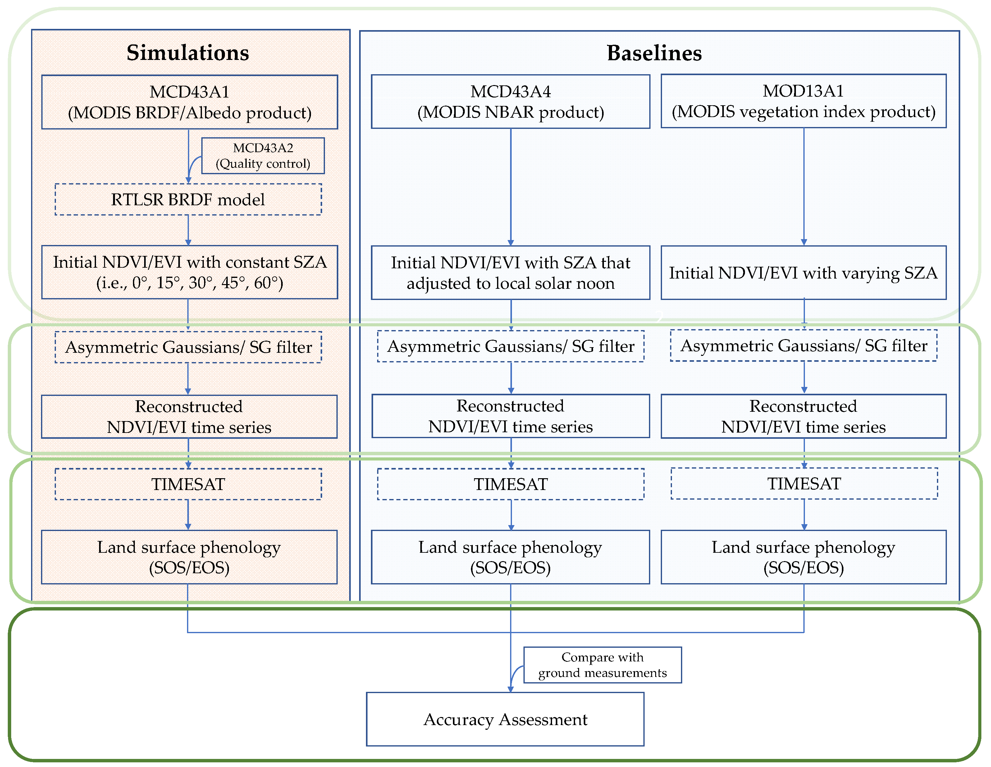
In this study, to compare LSPs derived from simulations with constant SZAs and from baseline products with inconsistent SZAs, four major processes are required, including NDVI/EVI time series simulation based on a kernel-driven model, NDVI/EVI time series reconstruction, land surface phenology derivation, and accuracy assessment (Figure 1).
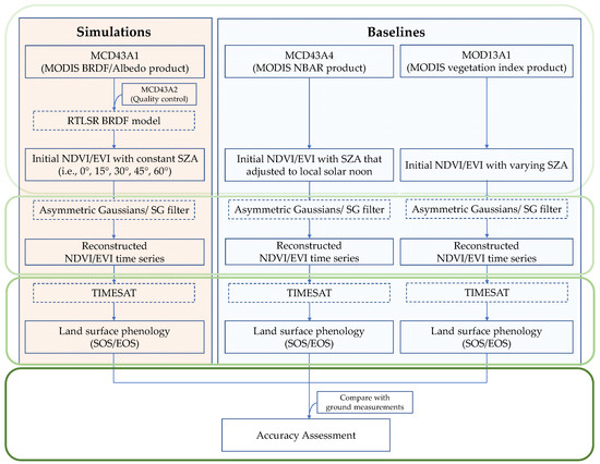
Figure 1.
The process chain of deriving LSP from simulations with constant SZAs and from baseline products with inconsistent SZAs. The green rectangles from top to the bottom represent NDVI/EVI time series simulation based on the kernel-driven model, NDVI/EVI time series reconstruction, land surface phenology derivation, and accuracy assessment, respectively. Blue solid rectangles are used products or derived results, while blue dashed rectangles are used models or integrated algorithms.
3.1. NDVI/EVI Time Series Simulation Based on the Kernel-Driven Model
We used the semiempirical RossThick-LiSparseReciprocal (RTLSR) BRDF model [12,61,72,73] to simulate reflectance under fixed illumination geometries. The RTLSR BRDF model simplifies the directional distribution of land surface reflectance as a linear combination of three components, i.e., the geometric optical scattering, volumetric optical scattering, and isotropic scattering [74,75,76,77], denoted by , and in Equation (1), respectively.
where is the reflectance in waveband under a designated viewing and illumination geometry. ,, and are spectrally dependent model parameters, with denoting an isotropic parameter, and , and serving as anisotropic parameters. and are the geometric optical scattering kernel and the volumetric optical scattering kernel, respectively [74,78,79]. , , and are the view zenith angle, solar zenith angle, and relative azimuth angle, respectively. Given that the MCD43A1 (BRDF) product provides the three model weighting parameters ,, and , RTLSR can be used to standardize the illumination geometry and generate comparable phenology metrics. The performance of the RTLSR BRDF model has been fully evaluated in previous studies [12,72,73], and it has been adopted as the standard model in operational MODIS BRDF/Albedo/NBAR products [61,69,70,80].
By verifying the longitude and latitude of the research site, we read the BRDF model parameters from the MCD43A1 (BRDF) product from 2001 to 2010. We also used the MCD43A2 (QA) product to remove the data contaminated by clouds, cloud shadows, and snow. The eligible BRDF model parameters were then put into the RTLSR BRDF model to simulate the surface reflectance with both the view zenith angle and the relative azimuth angle set to 0°, but the SZA was set to 0°, 15°, 30°, 45°, or 60° to test the solar angle effect. Although the real SZA at LSN in the Harvard Forest varies from 19° to 65°, variations in the illumination geometry come not only from the seasonal amplitude of the SZA at LSN [33] but also from the improved temporal resolution [34,35], satellite orbit drift [37,38], different data source integration [42,43,44], and terrain illumination [39,40,41], etc. Because of the abovementioned factors, the coupled impact could lead to a larger SZA range. Therefore, this study focused on SZAs spanning from 0° to 60°, with an interval of 15°. We start this range from 0° because we also want to analyze the impact of the hot spot, where the directional reflectance at nadir view is near to the illumination direction and therefore results in a spike in the reflectance profile [69,81]. Besides, we consider that the measured reflectance under SZAs larger than 60° is less accurate. We set a constant SZA throughout the year to eliminate the confounding effect of varying SZAs on deriving LSPs. To demonstrate that the impact of varying SZAs on the derived LSPs was not a special case in a certain year, we used a ten-year time series as a repeated annual experiment to strengthen the conclusion.
We selected NDVI and EVI in our study to derive LSP metrics because these two vegetation indices have been shown to be efficient indicators of vegetation growth conditions and have been largely used in phenology studies [13,14,15,16]. Based on Equations (2) and (3), the ten-year NDVI/EVI time series are obtained.
, and are the reflectance in the near-infrared band, red band, and blue band, respectively.
3.2. Reconstructing NDVI/EVI Time Series
LSP metrics were derived from continuous NDVI/EVI time series. However, the removal of unqualified values resulting from clouds, cloud shadows, and snow led to incomplete NDVI/EVI time series [82]. Therefore, we reconstructed the NDVI/EVI profiles in TIMESAT [83]. TIMESAT embeds three methods in its time-series-smoothing module, including adaptive Savitzky-Golay filter, asymmetric Gaussians, and double logistic functions [83], from which we chose both the SG filter and the asymmetric Gaussians. For NDVI/EVI time series with sufficient signals after removing unqualified values, the SG filter has the highest fidelity and is able to retain more details in the NDVI/EVI time series [84]; for NDVI/EVI time series with more than 3 consecutive months without signals, we used the asymmetric Gaussian due to its better performance in capturing the overall seasonal structure and in demonstrating less sensitivity to incomplete time-series data [85,86].
3.3. Deriving Land Surface Phenology
The reconstructed NDVI/EVI time series were then used to derive LSP metrics, including the start of season (SOS) and the end of season (EOS) [87], with SOS and EOS referring to the point at which the curve intersected a proportion of the seasonal amplitude measured from the left minimum and from the right minimum, respectively [51,88,89,90,91,92,93].
TIMESAT has been recognized as an efficient and robust software in phenology studies [94]. With its graphical user interface (GUI), TIMESAT is user-friendly by setting key parameters, e.g., the size of the moving window and the number of iterations [57]. To determine the SOS and EOS in the Harvard Forest from remote sensing data, we set the threshold at 0.5 to find the point at which the curve intersected 50% of the seasonal amplitude. For the SOS, the exposure of the understory reduces the NDVI at the beginning of each year, which extends the amplitude of the NDVI/EVI time series from the left side, so 50% of the amplitude closely matches the ground validations determined by BBRK30, as we introduced in Section 2.2.1. For the EOS, 50% of the amplitude from the right base level corresponds to the ground phenology metric of LFALL50.
3.4. Accuracy Assessment
The accuracy of the LSP derived from sensor data is measured by RMSE (root mean square error) and Spearman’s rank correlation coefficient. RMSE is used to measure the difference between the VI-derived LSP and the ground measurements, as shown in Equation (4).
where and denote the LSP metrics (SOS or EOS) derived from sensor data and ground measurements, respectively. N indicates the total year numbers in the time series, which is 10 in this study.
In contrast to RMSE, which measures how close the VI-derived LSPs are to ground measurements, Spearman’s rank correlation coefficient describes whether the trend of the 10-year time series in the VI-derived LSP aligns well with the trend in the ground-measured LSP. A large positive rank correlation coefficient indicates that the trend of the VI-derived LSP is consistent with the trend of the ground-measured LSP. Spearman’s rank correlation coefficient is calculated using Equation (5).
Here, ρ denotes the Spearman’s rank correlation coefficient; N is 10 in this study. is computed by sorting the VI-derived LSPs and ground-measured LSPs, calculating the difference between those two sorted arrays; the difference between corresponding elements in the two arrays is .
4. Results
4.1. NDVI and EVI Time Series
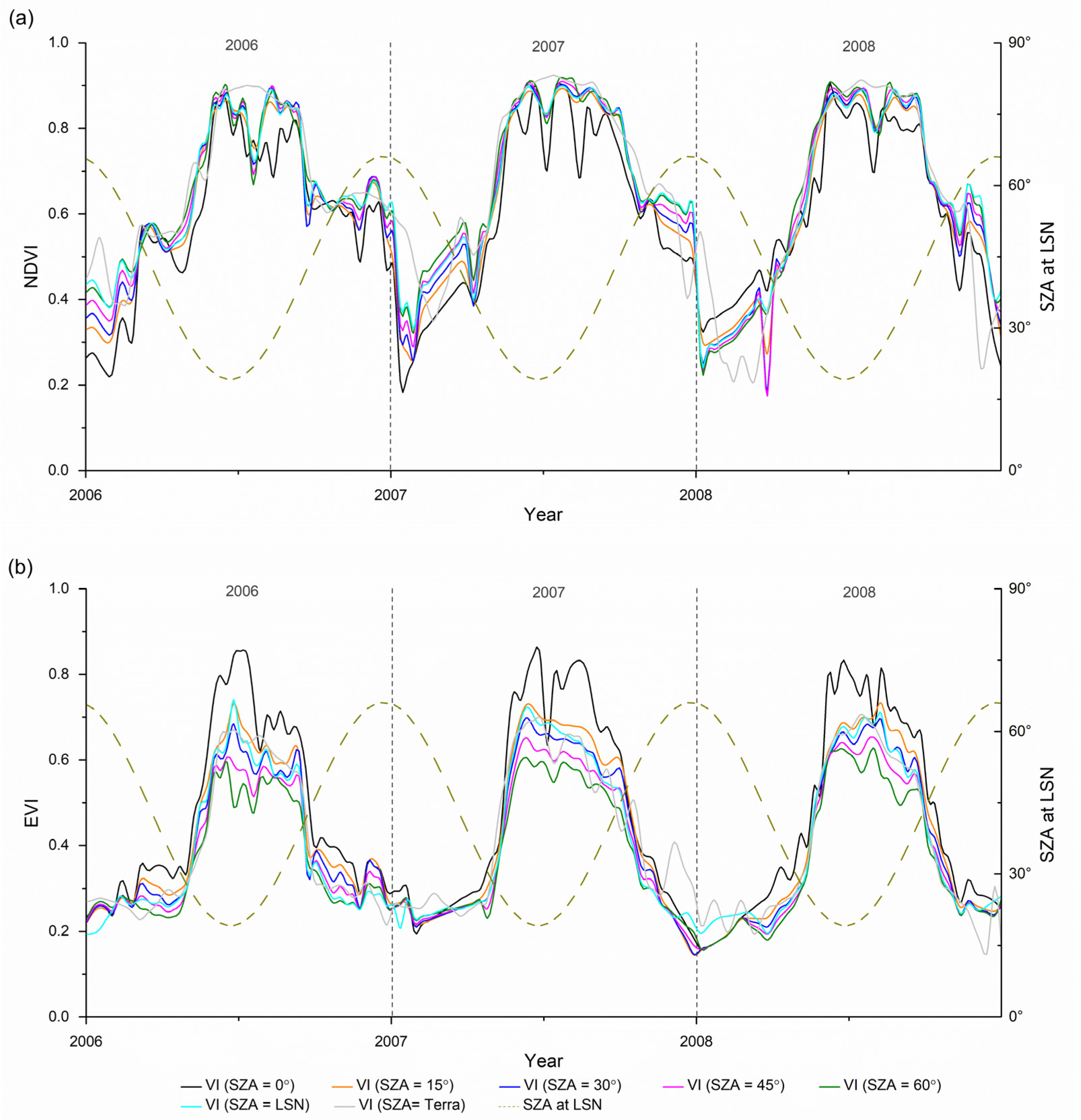
The ten-year NDVI/EVI time series in the Harvard Forest from 2001 to 2010 are consistent, suggesting that the vegetation conditions in this area are relatively stable, with no significant disturbances. Therefore, we use a three-year NDVI/EVI time series (2006 to 2008) to synchronize the need of showing details within a single year and of demonstrating the repeated pattern in the ten-year NDVI/EVI time series.
NDVI generally increases with SZA (Figure 2a), while EVI generally decreases with SZA (Figure 2b). The black lines in Figure 2 refer to the NDVI/EVI time series generated at the hot spot where the SZA equals the view zenith angle in this angle configuration, leading to a higher NDVI and a lower EVI compared to NDVI/EVI values under other angle configurations. Compared to the simulated NDVI/EVI time series with a constant SZA, the angle configuration of the NDVI/EVI time series from the MOD13A1 (VI) product shows less regularity (gray line) because of fewer constraints on the SZA. Although the NDVI/EVI time series from the MCD43A4 (NBAR) product (cyan line) is generated with view angle normalized to the nadir, the SZA still varies at LSN. Because the seasonal SZA shifts from 19° to 65° (dotted line), when the SZA at LSN approaches 15°, the NDVI/EVI time series from the MCD43A4 (NBAR) product (cyan line) is close to the time series simulated at 15° SZA (orange line); when the SZA is approximately 60°, the cyan line is close to the time series simulated at 60° SZA (green line) (Figure 2). This pattern not only demonstrates that the MODIS BRDF product has a high degree of accuracy in simulating the surface reflectance under a certain angle configuration but also shows the impact of varying SZAs on NDVI/EVI time series.
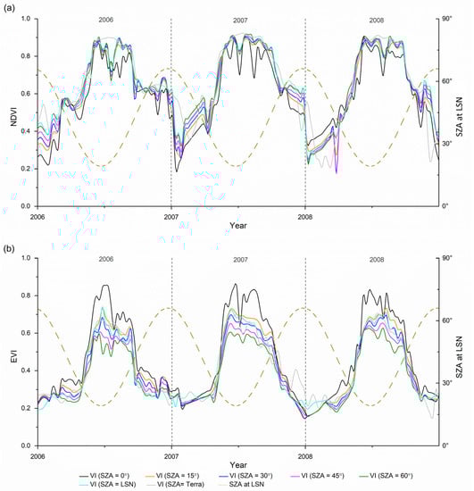
Figure 2.
(a) NDVI and (b) EVI time series in the Harvard Forest from 2006 to 2008. The NDVI/EVI profiles in black, orange, blue, magenta, and green represent the NDVI/EVI that are simulated with a view zenith angle and relative azimuth angle of 0° and with a constant SZA of 0°, 15°, 30°, 45° and 60°, respectively. The cyan line denotes the NDVI/EVI time series that is generated from the MCD43A4 (NBAR) product. The gray line is taken directly from the MOD13 (MODIS vegetation index product).
4.2. SOS Derived from NDVI and EVI Time Series
4.2.1. SOS Derived from NDVI Time Series
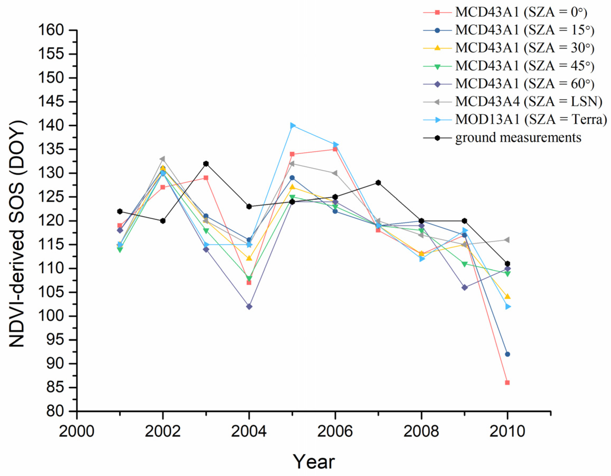
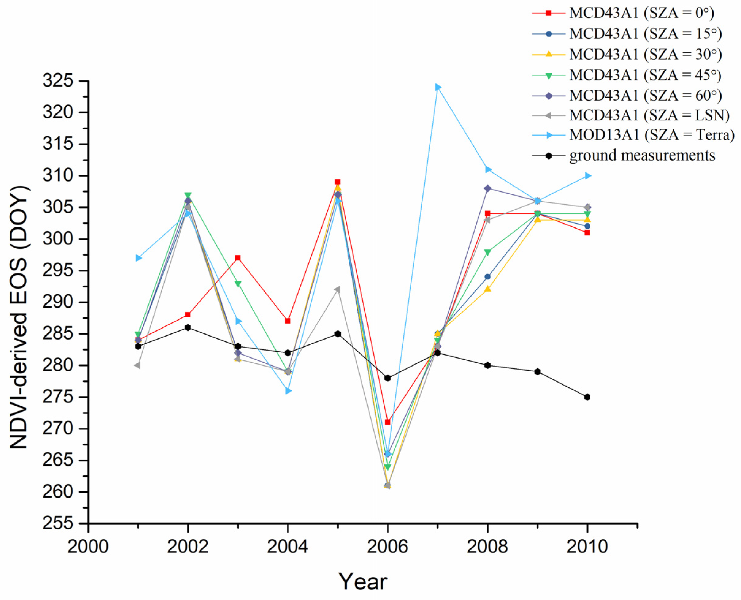
Figure 3 suggests that the NDVI-derived SOS tends to underestimate the SOS compared to ground measurements [95,96]. In Table 2, when SZA is 0° and 60°, the RMSE is high (11.4 and 10.8, respectively), which indicates discrepancies between NDVI-derived SOSs and ground-measured SOSs. The rank correlation between NDVI-derived SOSs and ground-measured SOSs is only 0.285 when SZA equals 60°, suggesting a large difference between the ground-measured SOS and the NDVI-derived SOS under 60° SZA in terms of the trend of SOS across the 10-year period. When the SZA equals 30°, the retrieved SOS has the best performance, exhibiting a lower RMSE (8.1) and a higher correlation (0.539). This could be explained by the fact that the actual SZA at the date of SOS in each year is close to 30°. Specifically, when averaging the corresponding SZA of each SOS, the 10-year averaged actual SZA is 28.23°, which is close to the 30° SZA we set in this angle configuration.
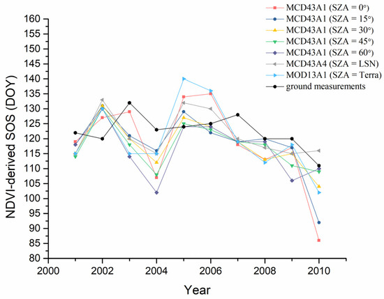
Figure 3.
SOS derived from the NDVI time series from 2001 to 2010. SZA = 0°, 15°, 30°, 45° and 60° denote the SOSs derived from the MCD43A1 (BRDF) product with a consistent angle configuration; SZA = LSN and SZA = Terra refer to SOSs derived from the MCD43A4 (NBAR) product and the MOD13A1 (VI) product, respectively.
Table 2.
Difference between the ground-observed and NDVI-derived SOS.
4.2.2. SOS Derived from EVI Time Series
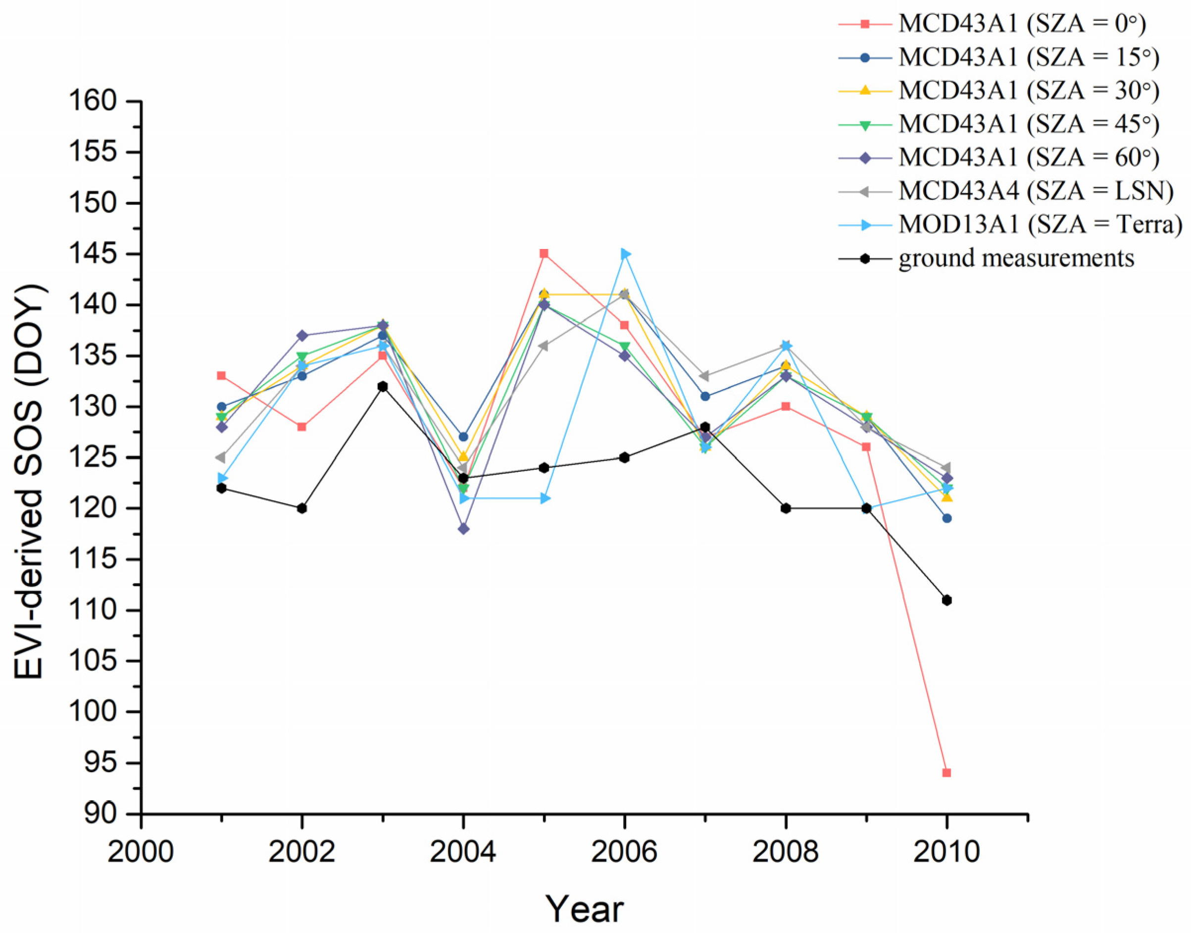
Figure 4 reveals that EVI-derived SOSs are delayed relative to the ground-measured SOSs, which is inverse to the pattern observed from NDVI-derived SOSs. EVI-derived SOSs show fewer discrepancies across different SZA configurations, with a maximum RMSE of 11.1 days, and a minimum RMSE of 10.0 days (Table 3). The Spearman’s rank correlation coefficient (ρ) also demonstrates a good rank correlation between EVI-derived SOSs and ground-measured SOSs, excluding SOSs retrieved under 60° SZA and retrieved directly from the MOD13A1 (VI) product.
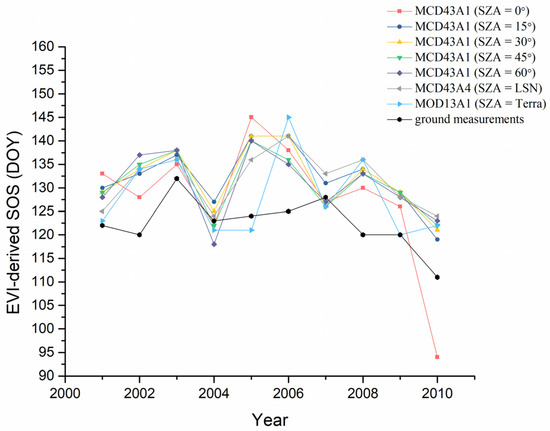
Figure 4.
SOS derived from the EVI time series from 2001 to 2010. SZA = 0°, 15°, 30°, 45° and 60° denote the SOSs derived from the MCD43A1 (BRDF) product with a consistent angle configuration; SZA = LSN and SZA = Terra refer to SOSs derived from the MCD43A4 (NBAR) product and the MOD13A1 (VI) product, respectively.
Table 3.
Difference between the ground-observed and EVI-derived SOS.
4.2.3. Comparison of SOS Derived from NDVI and EVI Time Series
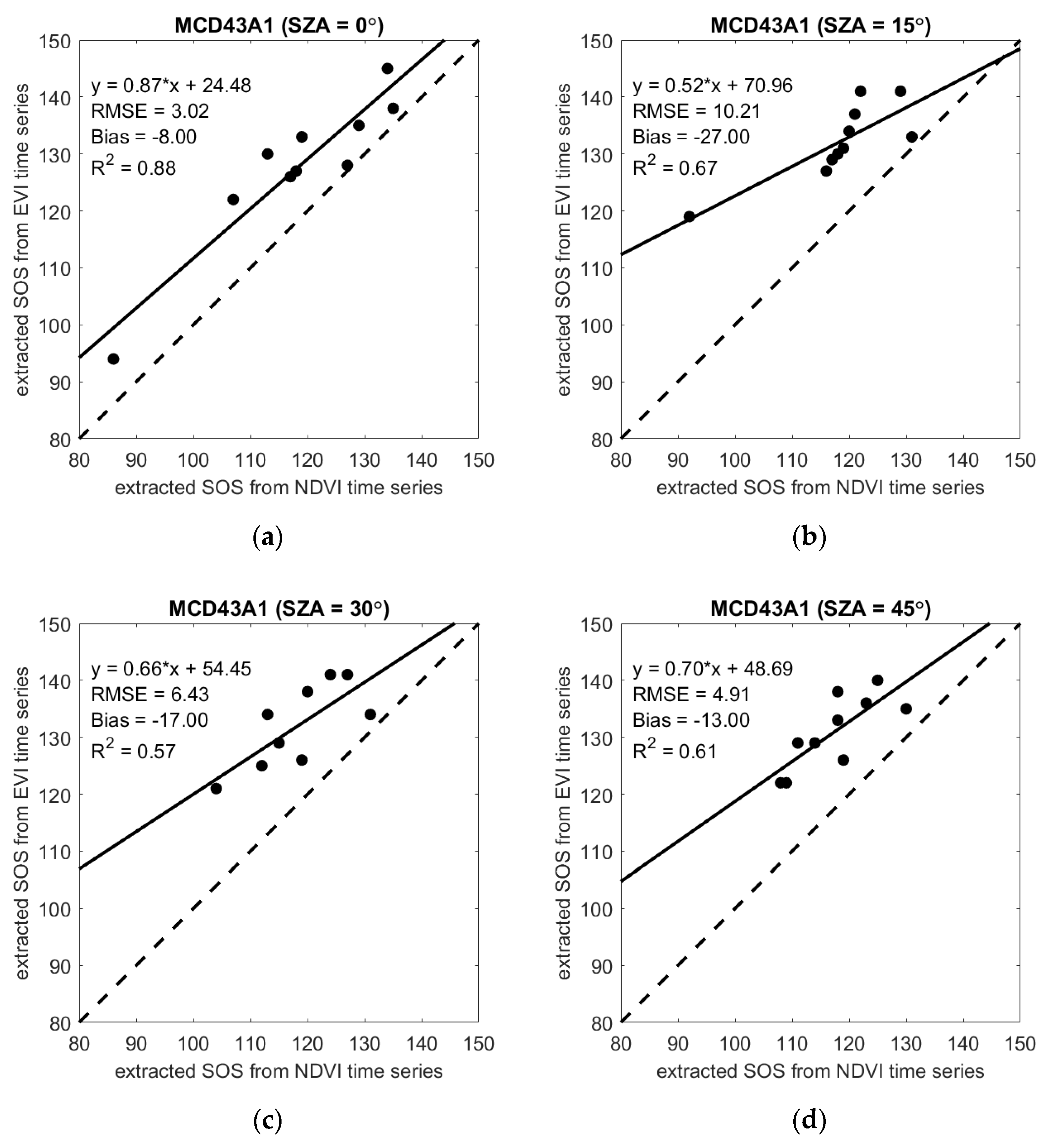
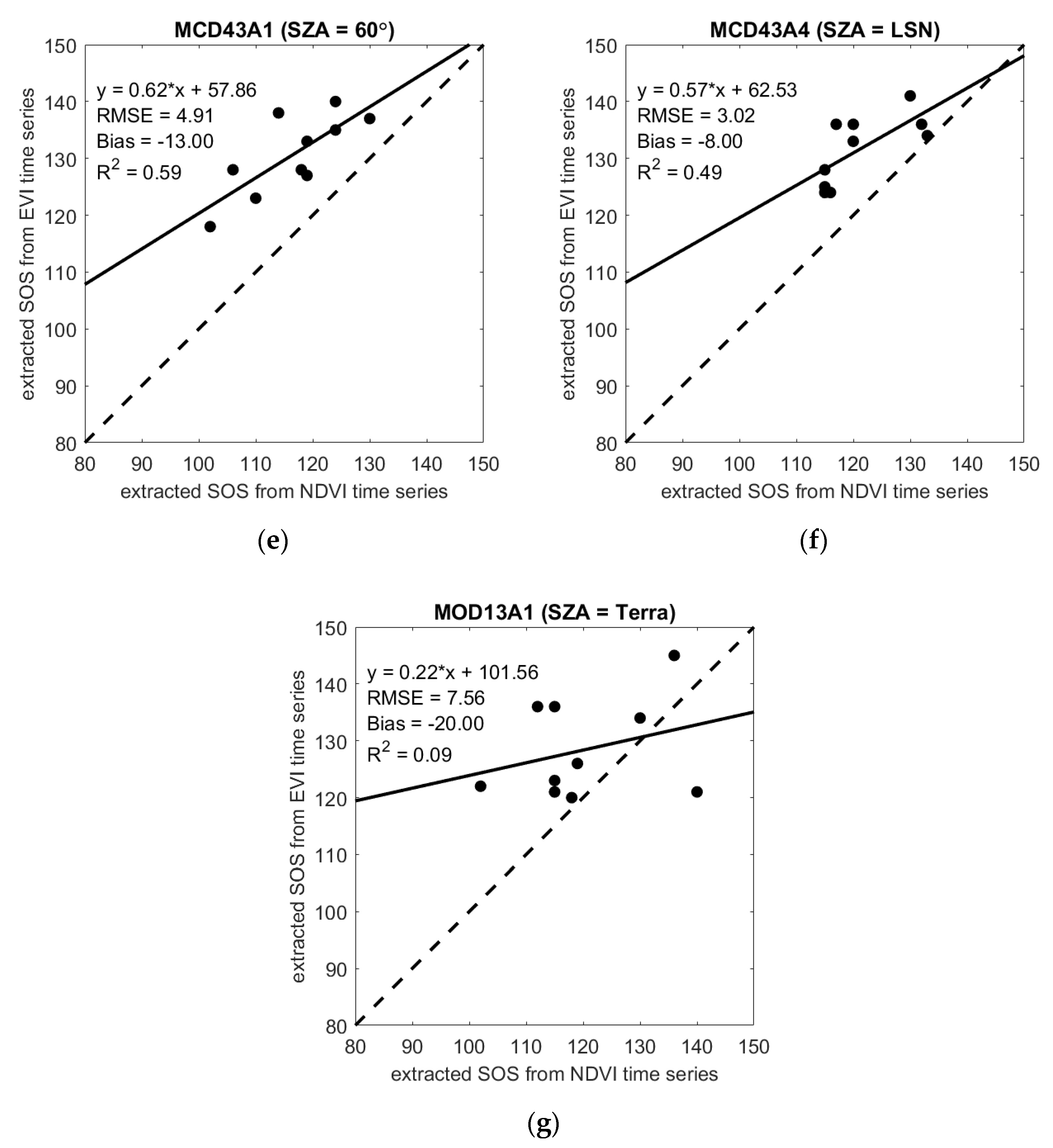
Comparisons of the SOSs derived from the NDVI and EVI time series from 2001 to 2010 are shown in Figure 5. The x-axis represents the NDVI-derived SOS, and the y-axis indicates the EVI-derived SOS. The SOSs derived from MCD43A1 (BRDF) product are distributed along the diagonal and exhibit a higher correlation (0.57 < R2 < 0.88), indicating that the NDVI-derived SOSs and EVI-derived SOSs under a constant SZA are relatively close; the SOSs derived from the MCD43A4 (NBAR) and MOD13A1 (VI) products show a relatively low correlation, with an R2 of 0.49 for the former and only 0.09 for the latter. In addition, the distribution of points occurs mainly above the diagonal line, suggesting that EVI-derived SOSs generally occur later than NDVI-derived SOSs.
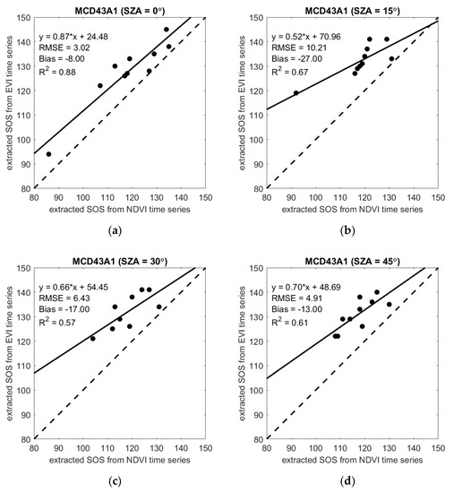
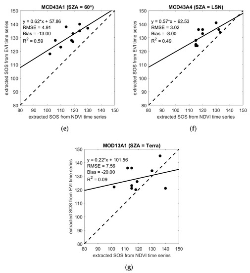
Figure 5.
Comparison of SOS derived from the NDVI and EVI time series from 2001 to 2010 when the SZA is (a) 0°; (b) 15°; (c) 30°; (d) 45°; (e) 60°; (f) at local solar noon; and (g) dependent on the observations of the Terra satellite. (a–e) are derived from the simulations, while (f,g) are from the MCD43A4 (NBAR) product and MOD13A1 (VI) product, respectively.
4.3. EOS Derived from NDVI and EVI Time Series
4.3.1. EOS Derived from NDVI Time Series
In contrast with NDVI-derived SOS, NDVI-derived EOS generally overestimates the EOS relative to that of the ground measurements, excluding 2006. From Table 4, the NDVI-derived EOS shows a large RMSE when the SZA equals 60°, indicating a poor performance of the simulated NDVI time series in deriving EOS under a large SZA. Compared to the rank correlation between NDVI-derived SOSs and ground-measured SOSs (Table 2), the rank correlation between NDVI-derived EOSs and ground-measured EOSs is low (Table 4), aligning well with the pattern shown in Figure 6, where the trend of ground-measured EOS over ten years shows less variation, yet the NDVI-derived EOS demonstrates drastic variation throughout the evaluated years.
Table 4.
Difference between the ground-observed and NDVI-derived EOS.
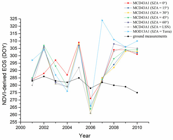
Figure 6.
EOS derived from the NDVI time series from 2001 to 2010. SZA = 0°, 15°, 30°, 45° and 60° denote the EOSs derived from the MCD43A1 (BRDF) product with a consistent angle configuration; SZA = LSN and SZA = Terra refer to EOSs derived from the MCD43A4 (NBAR) product and the MOD13A1 (VI) product, respectively.
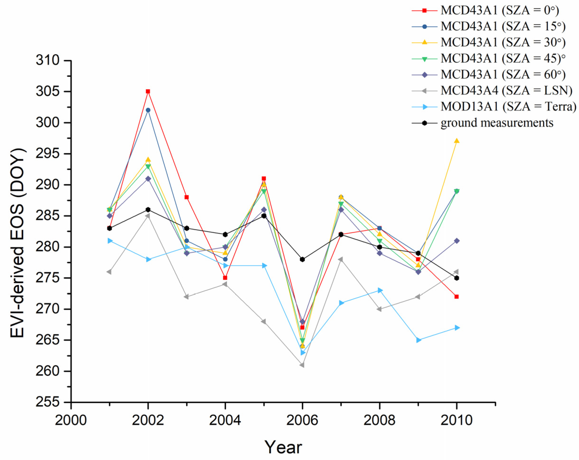
4.3.2. EOS Derived from EVI Time Series
The EOS derived from the MCD43A4 (NBAR) and MOD13A1 (VI) products are generally underestimated in contrast to the EOS derived from the simulated EVI time series under constant illumination geometry (Figure 7). Similar to NDVI-derived EOSs, EVI-derived EOSs are substantially advanced in 2006 relative to the ground-measured EOS, with an average underestimation of 13.4 days. From Table 4 and Table 5, the RMSE and Spearman’s rank correlation coefficients are generally improved in comparison with NDVI-derived EOSs, suggesting the better performance of the EVI time series to derive EOSs.
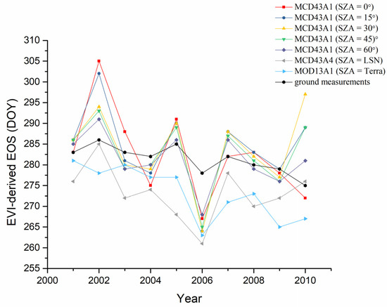
Figure 7.
EOS derived from the EVI time series from 2001 to 2010. SZA = 0°, 15°, 30°, 45° and 60° denote the EOSs derived from the MCD43A1 (BRDF) product with a consistent angle configuration; SZA = LSN and SZA = Terra refer to EOSs derived from the MCD43A4 (NBAR) product and the MOD13A1 (VI) product, respectively.
Table 5.
Difference between the ground-observed and EVI-derived EOS.
4.3.3. Comparison of EOS Derived from NDVI and EVI Time Series
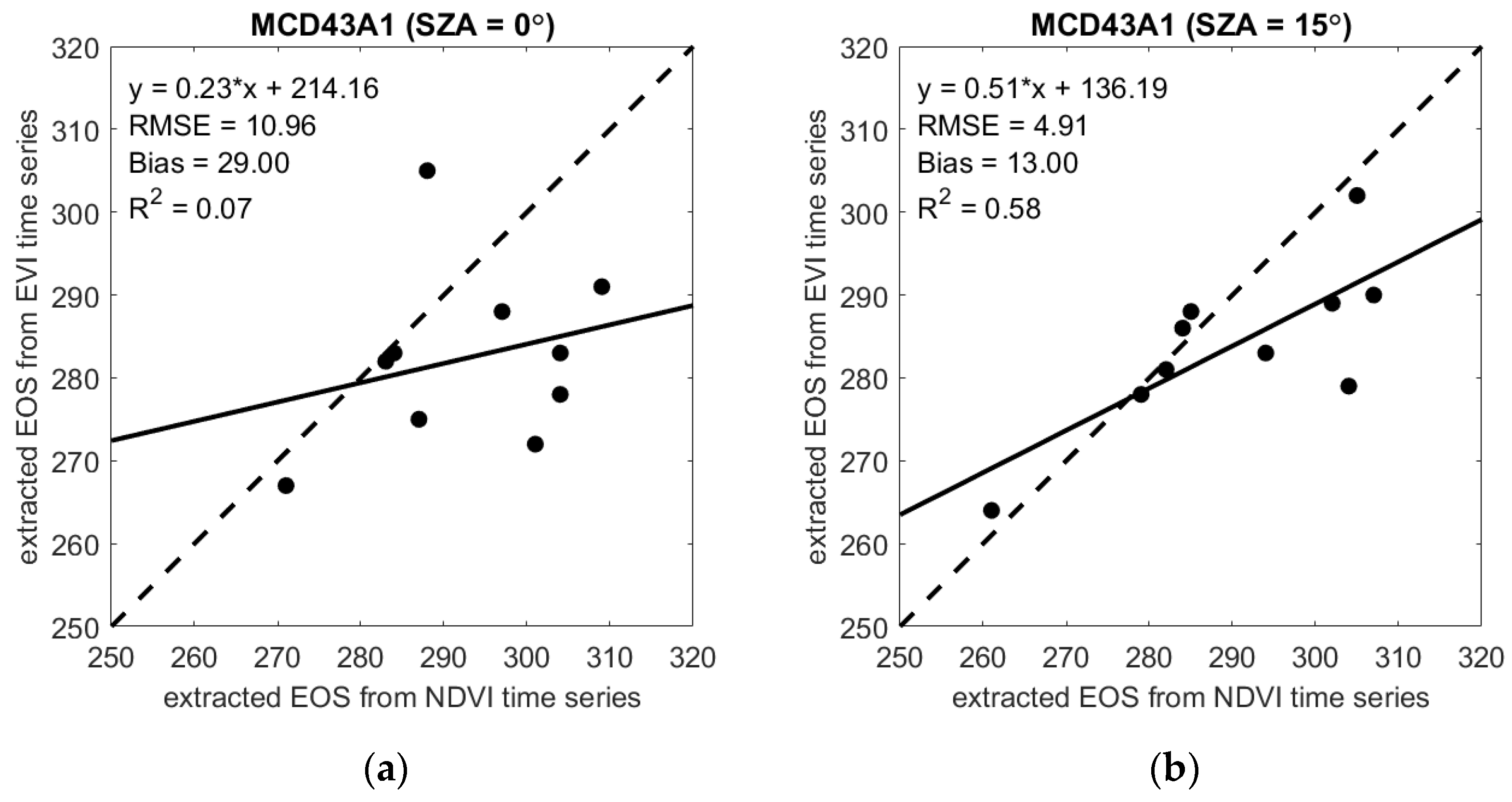
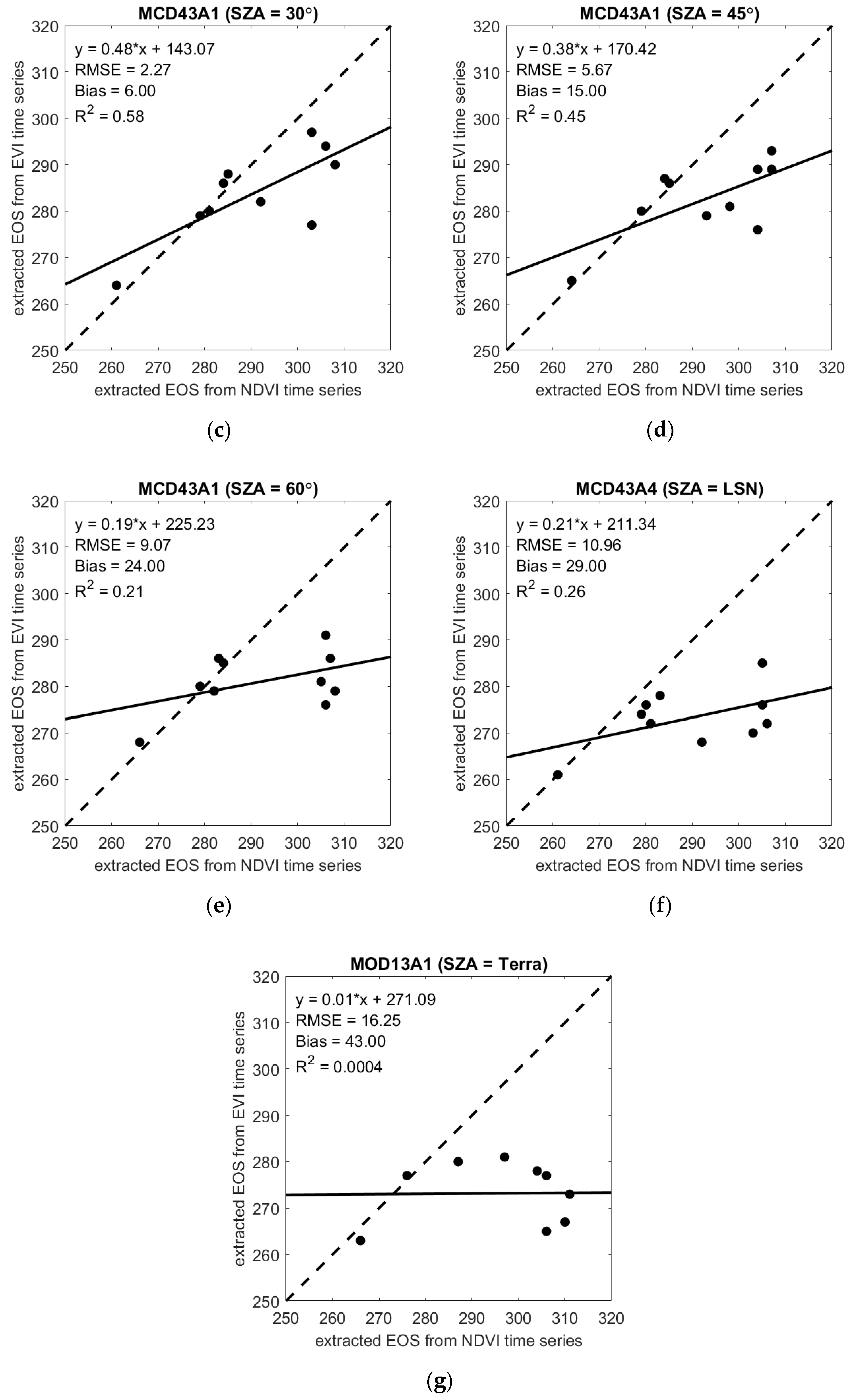
A comparison between NDVI-derived EOSs and EVI-derived EOSs is shown in Figure 8, with a poor correlation compared to VI-derived SOSs. When the SZA is within the range from 15° to 45°, 0.45 < R2 < 0.58, and when the SZA is 0° and 60°, R2 is 0.07 and 0.21, respectively. The R2 between retrieved EOSs from the MOD13 (VI) NDVI and the EVI time series is only 0.0004, indicating a compromised consistency. Additionally, the distribution of points is located below the diagonal, which indicates that EOSs derived from EVI are generally earlier than those derived from NDVI.


Figure 8.
Comparison of EOS derived from the NDVI and EVI time series from 2001 to 2010 when the SZA is (a) 0°; (b) 15°; (c) 30°; (d) 45°; (e) 60°; (f) at local solar noon; and (g) dependent on observations of the Terra satellite. (a–e) are derived from the simulations, while (f,g) are from the MCD43A4 (NBAR) product and the MOD13A1 (VI) product, respectively.
5. Discussion
5.1. NDVI and EVI Time Series
The NDVI and EVI time series depict similar seasonal variations in the deciduous Harvard Forest, but discrepancies still exist. First, EVI profiles are lower than NDVI profiles. Huete et al. [67] indicated that the reflectance of the red and blue bands in a phenological period were relatively stable, but the near-infrared band exhibited clear seasonal characteristics: when the growing season reached its peak, the near-infrared curve also reached its highest value, so NDVI would be larger than EVI under the same vegetation condition and geometric structure. Second, the EVI profile shows less fluctuation at the mature stage relative to the NDVI profile due to its improvement in reducing atmospheric impacts and the influence of soil background. Third, in each summer season, except for the NDVI/EVI profiles derived from the MOD13A1 (VI) product, other NDVI/EVI profiles show clear drops, especially lines at 0° because of the impact of the hot spot. This phenomenon appears every year, presumably due to the concentration of precipitation because the presence of clouds in the summer leads to a sharp decrease in the NDVI.
5.2. Comparison of VI-Derived Land Surface Phenology Metrics
We find a limited strength of remote sensing data in retrieving EOS compared to SOS, which is consistent with previous studies [22,24,95,97,98], irrespective of sensors or plant functional types [96]. Testa et al. [24] compared the NDVI and EVI-derived LSP metrics of French deciduous forests, pointing out that SOSs are more accurate (±10 days) than EOSs (±23 days). For the SOS, the results from both the NDVI and EVI time series are relatively close to the ground measurements, with absolute mean differences of 8.01 days for the former (Figure 3) and 9.07 days for the latter (Figure 4). The RMSE of the difference between VI-derived SOSs and ground-measured SOSs is less than 12 (Table 2 and Table 3). However, a considerable lag exists when deriving the EOS from NDVI time series, with 14.67 days as the absolute mean difference from the ground measurements across ten years (Figure 6). Table 4 also shows that the NDVI-derived EOS drastically overestimates the EOS compared to the ground-measured EOS, with a maximum RMSE of 33.7. Multiple reasons contribute to the uncertainty in retrieving EOS from remote sensing data, including longer and slower changes in canopy greenness in fall [97,98], the temporal resolution of sensor data [96], species and topography [99], and different sensitivities that different vegetation indices show to vegetate growth [100].
The LSP metrics derived from NDVI and EVI time series also show discrepancies. Specifically, NDVI-derived SOSs advance the green-up dates compared to the ground-measured SOSs (Figure 3), but delayed SOSs are retrieved from the EVI time series (Figure 4). This pattern is further verified in Figure 5, with the distribution of points essentially located above the diagonal, illustrating that the SOSs retrieved from EVI time series are later than those retrieved from NDVI time series [101,102]. For the VI-derived EOSs, the results derived from the EVI time series are generally earlier than those from the NDVI time series (Figure 8). Specifically, the EOSs derived from the NDVI time series overestimate the ground-measured EOSs (Figure 6), the EOSs derived from the simulated EVI time series under constant illumination geometries also overestimate, but the EOSs derived from EVI time series generated from baseline products (i.e., MCD43A4 (NBAR) and MOD13A1 (VI)) generally underestimate the ground-measured EOSs. Compared to the NDVI-derived EOS, the EVI-derived EOS has a better performance with a smaller RMSE and a higher Spearman’s rank correlation coefficient (Table 4 and Table 5), which echoes the previous finding that the LSP derived from different vegetation indices varies, suggesting different sensitivities of vegetation indices to vegetation growth [24,100].
5.3. Impacts from Illumination Geometry on Deriving Land Surface Phenology Metrics
The NDVI and EVI time series show an opposite pattern with increasing SZA: the larger the SZA, the higher the NDVI profiles, but the lower the EVI profiles. This result aligns well with previous studies [34,38]. The increase of SZA results in decreased reflectance in both red and near-infrared bands, but NDVI increases at large SZA because of a greater decrease in the red than in the near-infrared [103,104,105], while EVI decreases at large SZA because of greater NIR dependence [106,107,108]. In addition, the sensitivities of NDVI and EVI to varying SZAs are different. Specifically, EVI is more sensitive to varying SZAs than NDVI, especially in growing seasons, where the NDVI profiles are less scattered than the EVI profiles. The stronger sensitivity of EVI to varying SZAs echoes previous research conducted by Galvão et al. (2011). They compared 10 narrowband vegetation indices in terms of their sensitivity to view-illumination effects and found EVI was more anisotropic than NDVI. They also found shade fraction was negatively related to EVI. In this study, both view zenith angle and relative azimuth angle are set to 0, so shade fraction increases with the increase of SZA. Therefore, EVI decreases with the increase of SZA (Figure 2b).
The impact of varying SZAs on the NDVI/EVI time series leads to discrepancies in the retrieved LSP. For example, when using the NDVI time series to extract the SOS in the Harvard Forest in 2010, the results from the NDVI time series under a 0° SZA and from the MCD43A4 (NBAR) product are DOY 86 and DOY 116, respectively, exhibiting a difference of 30 days (Figure 3). In 2007, the EOS derived from the MOD13A1 (NDVI) product is DOY324, whereas the mean EOS of other products that take the influence of the SZA into account is DOY284, which is closer to the ground measurement of DOY 278 (Figure 6). Although the above evidence demonstrates that the SZA effect should be corrected uniformly when deriving LSP from NDVI/EVI time series, the different responses of the retrieved LSP to varying SZAs suggest the difficulty of applying a standard SZA correction method to all VI-derived LSPs. For example, the NDVI-derived SOS under a 30° SZA has the best performance of all the VI-derived SOSs, with an RMSE of 8.1 and a Spearman’s rank correlation coefficient of 0.539 (Table 2); however, the NDVI-derived EOS under a 30° SZA shows a large discrepancy relative to the corresponding ground-measured EOS, with an RMSE of 21.3 and a Spearman’s rank correlation coefficient of 0.321 (Table 4). This highlights the need of exploring how site-specific characteristics impact the correction of the SZA effect in future studies.
It is worth noting that we use MODIS products in this study because the MODIS BRDF/Albedo product provides a possibility to normalize the angle configurations based on the RTLSR BRDF model. However, for any dataset that has inconsistent angle configurations, the impact of inconsistent SZAs on the accuracy of retrieved LSPs should be considered.
5.4. Uncertainties
The VI-derived LSP under a set of constant SZAs is evaluated using ground observations, which raises the issue of scaling mismatch. This scaling issue has existed since the very beginning of remote sensing techniques, and satellite-based phenology studies were not immune to the spatial mismatch with the field data. However, the defects cannot obscure the virtues, satellite remote sensing products provide long-term, continuous, local- to global-scale, retrospective observations, which expands the horizon of traditional phenology [89,109,110]. Ground observations have also been widely used to validate satellite-derived LSP metrics [26,110,111]. In addition, most scaling issues come from the heterogeneity of the Earth’s surface [26,27,89]; however, a good relative consistency exists among species and among individuals within a species in this study area. Therefore, we consider that the data gathered in the Harvard Forest could be used to validate our results, especially as this dataset is mature and qualified [53,54].
A discrepancy also exists between ground LSP measured from the overstory and from the understory, separating the over- and understory would enable more accurate analysis of LSP [112,113]. But this study focuses on the discrepancy among LSP derived under different SZAs, and this discrepancy exists due to inherent biases in angle configurations, even if without comparing to ground measurements. Compared to ground validation data helps to quantify how LSP derived from different remote sensing products or derived under different angle configurations deviate from each other. Although we focus more on differences in the LSP metrics resulting from SZA effects instead of optimizing the method to derive the LSP metrics that are closest to the ground measurements in this study, the uncertainties due to potentially mismatched satellite-derived LSP and ground-measured LSP should be mentioned.
6. Conclusions
In this study, we demonstrat that changing SZAs not only influence the NDVI/EVI time series but also exerts a cascading effect on the retrieved LSP. BRDF parameters provided by the MCD43A1 (BRDF) product were used as inputs in the RTLSR BRDF model to simulate reflectance at a constant SZA configuration. The MCD43A4 (NBAR) and MOD13A1 (VI) products were used as baselines. Our results illustrate that both NDVI and EVI time series are sensitive to varying SZAs but in an opposite manner: NDVI increases with increasing SZAs, while EVI decreases. We also compared the retrieved LSP to ground measurements, finding limited strength of remote sensing data in retrieving EOS compared to retrieving SOS. Although NDVI and EVI have equivalent accuracy in deriving SOS, EVI demonstrates advantages in predicting EOS. The discrepancies between these two vegetation indices in terms of deriving LSP are also reflected in whether the retrieved phenology is advanced or delayed. Specifically, SOSs derived from NDVI time series are advanced, yet from EVI time series are delayed. However, EOSs derived from NDVI time series are delayed, and from simulated EVI time series under consistent illumination geometry are also delayed, but EOSs derived from baseline products (i.e., MCD43A4 (NBAR) and MOD13A1 (VI)) are generally advanced. Additionally, the LSP derived from varying illumination geometries could lead to a difference spanning from a few days to a month in this case study, which has important implications for normalizing the illumination geometries in deriving LSP from remote sensing data. End-users of multi-angle remote sensing products, therefore, are suggested to take the SZA effect into consideration.
Author Contributions
Conceptualization, Y.L., Z.J. and K.Z.; methodology, Y.L., Z.J. and Y.Z. (Yelu Zeng); software, Y.L. and Y.D.; formal analysis, Y.L., Z.J. and K.Z.; data curation, Y.Z. (Yelu Zeng), T.H. and L.C.; writing—original draft preparation, Y.L.; writing—review and editing, Z.J., K.Z., Y.Z. (Yuyu Zhou), X.Z., Y.D. and H.X.; funding acquisition, Z.J. All authors have read and agreed to the published version of the manuscript.
Funding
This research was funded by the Natural Science Foundation of China (No. 41971288 and 41571326).
Institutional Review Board Statement
Not applicable.
Informed Consent Statement
Not applicable.
Data Availability Statement
The remote sensing data that support the findings of this study are openly available on Google Earth Engine platform. The ground measurements are from the Harvard Forest Data Archive: https://harvardforest1.fas.harvard.edu/exist/apps/datasets/showData.html?id=HF003 (accessed on 1 October 2021). The dataset that supports the findings of this study is available from the corresponding author upon request.
Conflicts of Interest
The authors declare no conflict of interest.
Abbreviations
| NDVI | Normalized Difference Vegetation Index |
| EVI | Enhanced Vegetation Index |
| LSP | Land Surface Phenology |
| SOS | Start of Season |
| EOS | End of Season |
| DOY | Day of Year |
| SZA | Solar Zenith Angle |
| LSN | Local Solar Noon |
| BRDF | Bidirectional Reflectance Distribution Function |
| NBAR | Nadir BRDF-Adjusted Reflectance |
References
- Schwartz, M.D. Phenology: An Integrative Environmental Science, 2nd ed.; Kluwer Academic Publishers: Dordrecht, The Netherlands, 2003. [Google Scholar]
- Ryu, Y.; Lee, G.; Jeon, S.; Song, Y.; Kimm, H. Monitoring Multi-Layer Canopy Spring Phenology of Temperate Deciduous and Evergreen Forests Using Low-Cost Spectral Sensors. Remote Sens. Environ. 2014, 149, 227–238. [Google Scholar] [CrossRef]
- Helm, B.; Ben-Shlomo, R.; Sheriff, M.J.; Hut, R.A.; Foster, R.; Barnes, B.M.; Dominoni, D. Annual Rhythms That Underlie Phenology: Biological Time-Keeping Meets Environmental Change. Proc. R. Soc. B Biol. Sci. 2013, 280, 20130016. [Google Scholar] [CrossRef] [Green Version]
- Donaldson, J.R.; Lindroth, R.L. Effects of Variable Phytochemistry and Budbreak Phenology on Defoliation of Aspen during a Forest Tent Caterpillar Outbreak. Agric. For. Entomol. 2008, 10, 399–410. [Google Scholar] [CrossRef]
- Zhang, X.; Friedl, M.A.; Schaaf, C.B.; Strahler, A.H.; Hodges, J.C.F.; Gao, F.; Reed, B.C.; Huete, A. Monitoring Vegetation Phenology Using MODIS. Remote Sens. Environ. 2003, 84, 471–475. [Google Scholar] [CrossRef]
- Peñuelas, J.; Rutishauser, T.; Filella, I. Phenology Feedbacks on Climate Change. Science 2009, 324, 887–888. [Google Scholar] [CrossRef] [PubMed] [Green Version]
- Li, X.; Zhou, Y.; Meng, L.; Asrar, G.; Sapkota, A.; Coates, F. Characterizing the Relationship between Satellite Phenology and Pollen Season: A Case Study of Birch. Remote Sens. Environ. 2019, 222, 267–274. [Google Scholar] [CrossRef]
- Sapkota, A.; Dong, Y.; Li, L.; Asrar, G.; Zhou, Y.; Li, X.; Coates, F.; Spanier, A.J.; Matz, J.; Bielory, L.; et al. Association Between Changes in Timing of Spring Onset and Asthma Hospitalization in Maryland. JAMA Netw. Open 2020, 3, e207551. [Google Scholar] [CrossRef]
- Chen, J.M.; Menges, C.H.; Leblanc, S.G. Global Mapping of Foliage Clumping Index Using Multi-Angular Satellite Data. Remote Sens. Environ. 2005, 97, 447–457. [Google Scholar] [CrossRef]
- Jiao, Z.; Dong, Y.; Schaaf, C.B.; Chen, J.M.; Román, M.; Wang, Z.; Zhang, H.; Ding, A.; Erb, A.; Hill, M.J.; et al. An Algorithm for the Retrieval of the Clumping Index (CI) from the MODIS BRDF Product Using an Adjusted Version of the Kernel-Driven BRDF Model. Remote Sens. Environ. 2018, 209, 594–611. [Google Scholar] [CrossRef]
- Cui, L.; Jiao, Z.; Dong, Y.; Sun, M.; Zhang, X.; Yin, S.; Ding, A.; Chang, Y.; Guo, J.; Xie, R. Estimating Forest Canopy Height Using MODIS BRDF Data Emphasizing Typical-Angle Reflectances. Remote Sens. 2019, 11, 2239. [Google Scholar] [CrossRef] [Green Version]
- Jiao, Z.; Hill, M.J.; Schaaf, C.B.; Zhang, H.; Wang, Z.; Li, X. An Anisotropic Flat Index (AFX) to Derive BRDF Archetypes from MODIS. Remote Sens. Environ. 2014, 141, 168–187. [Google Scholar] [CrossRef]
- Galvão, L.S.; Breunig, F.M.; Teles, T.S.; Gaida, W.; Balbinot, R. Investigation of Terrain Illumination Effects on Vegetation Indices and VI-Derived Phenological Metrics in Subtropical Deciduous Forests. GISci. Remote Sens. 2016, 53, 360–381. [Google Scholar] [CrossRef]
- Karkauskaite, P.; Tagesson, T.; Fensholt, R. Evaluation of the Plant Phenology Index (PPI), NDVI and EVI for Start-of-Season Trend Analysis of the Northern Hemisphere Boreal Zone. Remote Sens. 2017, 9, 485. [Google Scholar] [CrossRef] [Green Version]
- Peng, D.; Wu, C.; Li, C.; Zhang, X.; Liu, Z.; Ye, H.; Luo, S.; Liu, X.; Hu, Y.; Fang, B. Spring Green-up Phenology Products Derived from MODIS NDVI and EVI: Intercomparison, Interpretation and Validation Using National Phenology Network and AmeriFlux Observations. Ecol. Indic. 2017, 77, 323–336. [Google Scholar] [CrossRef]
- Tan, B.; Morisette, J.T.; Wolfe, R.E.; Gao, F.; Ederer, G.A.; Nightingale, J.; Pedelty, J.A. Vegetation Phenology Metrics Derived from Temporally Smoothed and Gap-Filled MODIS Data. In Proceedings of the IGARSS 2008 IEEE International Geoscience and Remote Sensing Symposium, Boston, MA, USA, 6–11 July 2008; Volume 3, pp. III-593–III-596. [Google Scholar]
- Li, X.; Zhou, Y.; Meng, L.; Asrar, G.R.; Lu, C.; Wu, Q. A Dataset of 30 m Annual Vegetation Phenology Indicators (1985–2015) in Urban Areas of the Conterminous United States. Earth Syst. Sci. Data Online 2019, 11, 881–894. [Google Scholar] [CrossRef] [Green Version]
- Gao, F.; Anderson, M.; Daughtry, C.; Karnieli, A.; Hively, D.; Kustas, W. A Within-Season Approach for Detecting Early Growth Stages in Corn and Soybean Using High Temporal and Spatial Resolution Imagery. Remote Sens. Environ. 2020, 242, 111752. [Google Scholar] [CrossRef]
- Xie, Y.; Wilson, A.M. Change Point Estimation of Deciduous Forest Land Surface Phenology. Remote Sens. Environ. 2020, 240, 111698. [Google Scholar] [CrossRef]
- Zhao, K.; Wulder, M.A.; Hu, T.; Bright, R.; Wu, Q.; Qin, H.; Li, Y.; Toman, E.; Mallick, B.; Zhang, X.; et al. Detecting Change-Point, Trend, and Seasonality in Satellite Time Series Data to Track Abrupt Changes and Nonlinear Dynamics: A Bayesian Ensemble Algorithm. Remote Sens. Environ. 2019, 232, 111181. [Google Scholar] [CrossRef]
- Li, X.; Zhou, Y.; Asrar, G.R.; Meng, L. Characterizing Spatiotemporal Dynamics in Phenology of Urban Ecosystems Based on Landsat Data. Sci. Total Environ. 2017, 605–606, 721–734. [Google Scholar] [CrossRef] [PubMed]
- Jeong, S.-J.; Schimel, D.; Frankenberg, C.; Drewry, D.T.; Fisher, J.B.; Verma, M.; Berry, J.A.; Lee, J.-E.; Joiner, J. Application of Satellite Solar-Induced Chlorophyll Fluorescence to Understanding Large-Scale Variations in Vegetation Phenology and Function over Northern High Latitude Forests. Remote Sens. Environ. 2017, 190, 178–187. [Google Scholar] [CrossRef]
- Motohka, T.; Nasahara, K.N.; Oguma, H.; Tsuchida, S. Applicability of Green-Red Vegetation Index for Remote Sensing of Vegetation Phenology. Remote Sens. 2010, 2, 2369–2387. [Google Scholar] [CrossRef] [Green Version]
- Testa, S.; Soudani, K.; Boschetti, L.; Borgogno Mondino, E. MODIS-Derived EVI, NDVI and WDRVI Time Series to Estimate Phenological Metrics in French Deciduous Forests. Int. J. Appl. Earth Obs. Geoinf. 2018, 64, 132–144. [Google Scholar] [CrossRef]
- Fu, Y.H.; Piao, S.; de Beeck, M.O.; Cong, N.; Zhao, H.; Zhang, Y.; Menzel, A.; Janssens, I.A. Recent Spring Phenology Shifts in Western Central Europe Based on Multiscale Observations. Glob. Ecol. Biogeogr. 2014, 23, 1255–1263. [Google Scholar] [CrossRef]
- Liang, L.; Schwartz, M.D.; Fei, S. Validating Satellite Phenology through Intensive Ground Observation and Landscape Scaling in a Mixed Seasonal Forest. Remote Sens. Environ. 2011, 115, 143–157. [Google Scholar] [CrossRef]
- Zhang, X.; Wang, J.; Gao, F.; Liu, Y.; Schaaf, C.; Friedl, M.; Yu, Y.; Jayavelu, S.; Gray, J.; Liu, L.; et al. Exploration of Scaling Effects on Coarse Resolution Land Surface Phenology. Remote Sens. Environ. 2017, 190, 318–330. [Google Scholar] [CrossRef] [Green Version]
- Zhang, X.; Friedl, M.A.; Schaaf, C.B. Sensitivity of Vegetation Phenology Detection to the Temporal Resolution of Satellite Data. Int. J. Remote Sens. 2009, 30, 2061–2074. [Google Scholar] [CrossRef]
- Klosterman, S.; Melaas, E.; Wang, J.A.; Martinez, A.; Frederick, S.; O’Keefe, J.; Orwig, D.A.; Wang, Z.; Sun, Q.; Schaaf, C.; et al. Fine-Scale Perspectives on Landscape Phenology from Unmanned Aerial Vehicle (UAV) Photography. Agric. For. Meteorol. 2018, 248, 397–407. [Google Scholar] [CrossRef]
- Nasahara, K.N.; Nagai, S. Review: Development of an in situ Observation Network for Terrestrial Ecological Remote Sensing: The Phenological Eyes Network (PEN). Ecol. Res. 2015, 30, 211–223. [Google Scholar] [CrossRef]
- Richardson, A.D.; Hufkens, K.; Milliman, T.; Aubrecht, D.M.; Chen, M.; Gray, J.M.; Johnston, M.R.; Keenan, T.F.; Klosterman, S.T.; Kosmala, M.; et al. Tracking Vegetation Phenology across Diverse North American Biomes Using PhenoCam Imagery. Sci. Data 2018, 5, 180028. [Google Scholar] [CrossRef]
- Hu, T.; Zhao, T.; Zhao, K.; Shi, J. A Continuous Global Record of Near-Surface Soil Freeze/Thaw Status from AMSR-E and AMSR2 Data. Int. J. Remote Sens. 2019, 40, 6993–7016. [Google Scholar] [CrossRef]
- Gao, F.; He, T.; Masek, J.G.; Shuai, Y.; Schaaf, C.B.; Wang, Z. Angular Effects and Correction for Medium Resolution Sensors to Support Crop Monitoring. IEEE J. Sel. Top. Appl. Earth Obs. Remote Sens. 2014, 7, 4480–4489. [Google Scholar] [CrossRef]
- Fensholt, R.; Sandholt, I.; Stisen, S.; Tucker, C. Analysing NDVI for the African Continent Using the Geostationary Meteosat Second Generation SEVIRI Sensor. Remote Sens. Environ. 2006, 101, 212–229. [Google Scholar] [CrossRef]
- Fensholt, R.; Sandholt, I.; Proud, S.R.; Stisen, S.; Rasmussen, M.O. Assessment of MODIS Sun-Sensor Geometry Variations Effect on Observed NDVI Using MSG SEVIRI Geostationary Data. Int. J. Remote Sens. 2010, 31, 6163–6187. [Google Scholar] [CrossRef]
- Lindström, J.; Eklundh, L.; Holst, J.; Holst, U. Influence of Solar Zenith Angles on Observed Trends in the NOAA/NASA 8-km Pathfinder Normalized Difference Vegetation Index over the African Sahel. Int. J. Remote Sens. 2006, 27, 1973–1991. [Google Scholar] [CrossRef]
- Roy, D.P.; Li, Z.; Zhang, H.K.; Huang, H. A Conterminous United States Analysis of the Impact of Landsat 5 Orbit Drift on the Temporal Consistency of Landsat 5 Thematic Mapper Data. Remote Sens. Environ. 2020, 240, 111701. [Google Scholar] [CrossRef]
- Galvão, L.S.; de Souza, A.A.; Breunig, F.M. A Hyperspectral Experiment over Tropical Forests Based on the EO-1 Orbit Change and PROSAIL Simulation. GISci. Remote Sens. 2020, 57, 74–90. [Google Scholar] [CrossRef]
- Hao, D.; Wen, J.; Xiao, Q.; Wu, S.; Lin, X.; Dou, B.; You, D.; Tang, Y. Simulation and Analysis of the Topographic Effects on Snow-Free Albedo over Rugged Terrain. Remote Sens. 2018, 10, 278. [Google Scholar] [CrossRef] [Green Version]
- Matsushita, B.; Yang, W.; Chen, J.; Onda, Y.; Qiu, G. Sensitivity of the Enhanced Vegetation Index (EVI) and Normalized Difference Vegetation Index (NDVI) to Topographic Effects: A Case Study in High-Density Cypress Forest. Sensors 2007, 7, 2636–2651. [Google Scholar] [CrossRef] [Green Version]
- Teles, T.S.; Galvão, L.S.; Breunig, F.M.; Balbinot, R.; Gaida, W. Relationships between MODIS Phenological Metrics, Topographic Shade, and Anomalous Temperature Patterns in Seasonal Deciduous Forests of South Brazil. Int. J. Remote Sens. 2015, 36, 4501–4518. [Google Scholar] [CrossRef]
- Bolton, D.K.; Gray, J.M.; Melaas, E.K.; Moon, M.; Eklundh, L.; Friedl, M.A. Continental-Scale Land Surface Phenology from Harmonized Landsat 8 and Sentinel-2 Imagery. Remote Sens. Environ. 2020, 240, 111685. [Google Scholar] [CrossRef]
- Franch, B.; Vermote, E.; Skakun, S.; Roger, J.-C.; Masek, J.; Ju, J.; Villaescusa-Nadal, J.L.; Santamaria-Artigas, A. A Method for Landsat and Sentinel 2 (HLS) BRDF Normalization. Remote Sens. 2019, 11, 632. [Google Scholar] [CrossRef] [Green Version]
- Griffiths, P.; Nendel, C.; Hostert, P. Intra-Annual Reflectance Composites from Sentinel-2 and Landsat for National-Scale Crop and Land Cover Mapping. Remote Sens. Environ. 2019, 220, 135–151. [Google Scholar] [CrossRef]
- Berman, E.E.; Graves, T.A.; Mikle, N.L.; Merkle, J.A.; Johnston, A.N.; Chong, G.W. Comparative Quality and Trend of Remotely Sensed Phenology and Productivity Metrics across the Western United States. Remote Sens. 2020, 12, 2538. [Google Scholar] [CrossRef]
- Kowalski, K.; Senf, C.; Hostert, P.; Pflugmacher, D. Characterizing Spring Phenology of Temperate Broadleaf Forests Using Landsat and Sentinel-2 Time Series. Int. J. Appl. Earth Obs. Geoinf. 2020, 92, 102172. [Google Scholar] [CrossRef]
- Bhandari, S.; Phinn, S.; Gill, T. Assessing Viewing and Illumination Geometry Effects on the MODIS Vegetation Index (MOD13Q1) Time Series: Implications for Monitoring Phenology and Disturbances in Forest Communities in Queensland, Australia. Int. J. Remote Sens. 2011, 32, 7513–7538. [Google Scholar] [CrossRef]
- Ji, L.; Brown, J.F. Effect of NOAA Satellite Orbital Drift on AVHRR-Derived Phenological Metrics. Int. J. Appl. Earth Obs. Geoinf. 2017, 62, 215–223. [Google Scholar] [CrossRef]
- Breunig, F.M.; Galvão, L.S.; dos Santos, J.R.; Gitelson, A.A.; de Moura, Y.M.; Teles, T.S.; Gaida, W. Spectral Anisotropy of Subtropical Deciduous Forest Using MISR and MODIS Data Acquired under Large Seasonal Variation in Solar Zenith Angle. Int. J. Appl. Earth Obs. Geoinf. 2015, 35, 294–304. [Google Scholar] [CrossRef]
- Ma, X.; Huete, A.; Tran, N.N. Interaction of Seasonal Sun-Angle and Savanna Phenology Observed and Modelled Using MODIS. Remote Sens. 2019, 11, 1398. [Google Scholar] [CrossRef] [Green Version]
- Xin, Q.; Broich, M.; Zhu, P.; Gong, P. Modeling Grassland Spring Onset across the Western United States Using Climate Variables and MODIS-Derived Phenology Metrics. Remote Sens. Environ. 2015, 161, 63–77. [Google Scholar] [CrossRef]
- O’Keefe, J. Phenology of Woody Species at Harvard Forest since 1990. Harvard Forest Data Archive: HF003. Available online: https://harvardforest1.fas.harvard.edu/exist/apps/datasets/showData.html?id=HF003 (accessed on 1 October 2021).
- Friedl, M.A.; Gray, J.M.; Melaas, E.K.; Richardson, A.D.; Hufkens, K.; Keenan, T.F.; Bailey, A.; O’Keefe, J. A Tale of Two Springs: Using Recent Climate Anomalies to Characterize the Sensitivity of Temperate Forest Phenology to Climate Change. Environ. Res. Lett. 2014, 9, 054006. [Google Scholar] [CrossRef]
- Keenan, T.F.; Gray, J.; Friedl, M.A.; Toomey, M.; Bohrer, G.; Hollinger, D.Y.; Munger, J.W.; O’Keefe, J.; Schmid, H.P.; Wing, I.S.; et al. Net Carbon Uptake Has Increased through Warming-Induced Changes in Temperate Forest Phenology. Nat. Clim. Chang. 2014, 4, 598–604. [Google Scholar] [CrossRef]
- Keenan, T.F.; Davidson, E.A.; Munger, J.W.; Richardson, A.D. Rate My Data: Quantifying the Value of Ecological Data for the Development of Models of the Terrestrial Carbon Cycle. Ecol. Appl. 2013, 23, 273–286. [Google Scholar] [CrossRef] [Green Version]
- Xu, H.; Twine, T.E.; Yang, X. Evaluating Remotely Sensed Phenological Metrics in a Dynamic Ecosystem Model. Remote Sens. 2014, 6, 4660–4686. [Google Scholar] [CrossRef] [Green Version]
- Keenan, T.F.; Richardson, A.D. The Timing of Autumn Senescence Is Affected by the Timing of Spring Phenology: Implications for Predictive Models. Glob. Chang. Biol. 2015, 21, 2634–2641. [Google Scholar] [CrossRef] [PubMed] [Green Version]
- Hadley, J.L.; O’Keefe, J.; Munger, J.W.; Hollinger, D.Y.; Richardson, A.D. Phenology of Forest-Atmosphere Carbon Exchange for Deciduous and Coniferous Forests in Southern and Northern New England. In Phenology of Ecosystem Processes; Springer: New York, NY, USA, 2009; pp. 119–141. [Google Scholar]
- Richardson, A.D.; Hollinger, D.Y.; Dail, D.B.; Lee, J.T.; Munger, J.W.; O’keefe, J. Influence of Spring Phenology on Seasonal and Annual Carbon Balance in Two Contrasting New England Forests. Tree Physiol. 2009, 29, 321–331. [Google Scholar] [CrossRef]
- Yang, X.; Mustard, J.F.; Tang, J.; Xu, H. Regional-Scale Phenology Modeling Based on Meteorological Records and Remote Sensing Observations. J. Geophys. Res. Biogeosci. 2012, 117. [Google Scholar] [CrossRef]
- Schaaf, C.B.; Gao, F.; Strahler, A.H.; Lucht, W.; Li, X.; Tsang, T.; Strugnell, N.C.; Zhang, X.; Jin, Y.; Muller, J.-P.; et al. First Operational BRDF, Albedo Nadir Reflectance Products from MODIS. Remote Sens. Environ. 2002, 83, 135–148. [Google Scholar] [CrossRef] [Green Version]
- Wang, Z.; Schaaf, C.B.; Strahler, A.H.; Chopping, M.J.; Román, M.O.; Shuai, Y.; Woodcock, C.E.; Hollinger, D.Y.; Fitzjarrald, D.R. Evaluation of MODIS Albedo Product (MCD43A) over Grassland, Agriculture and Forest Surface Types during Dormant and Snow-Covered Periods. Remote Sens. Environ. 2014, 140, 60–77. [Google Scholar] [CrossRef] [Green Version]
- Shuai, Y.; Schaaf, C.B.; Strahler, A.H.; Liu, J.; Jiao, Z. Quality Assessment of BRDF/Albedo Retrievals in MODIS Operational System. Geophys. Res. Lett. 2008, 35. [Google Scholar] [CrossRef]
- Jin, H.; Eklundh, L. A Physically Based Vegetation Index for Improved Monitoring of Plant Phenology. Remote Sens. Environ. 2014, 152, 512–525. [Google Scholar] [CrossRef]
- Liu, L.; Liang, L.; Schwartz, M.D.; Donnelly, A.; Wang, Z.; Schaaf, C.B.; Liu, L. Evaluating the Potential of MODIS Satellite Data to Track Temporal Dynamics of Autumn Phenology in a Temperate Mixed Forest. Remote Sens. Environ. 2015, 160, 156–165. [Google Scholar] [CrossRef]
- Ahl, D.E.; Gower, S.T.; Burrows, S.N.; Shabanov, N.V.; Myneni, R.B.; Knyazikhin, Y. Monitoring Spring Canopy Phenology of a Deciduous Broadleaf Forest Using MODIS. Remote Sens. Environ. 2006, 104, 88–95. [Google Scholar] [CrossRef] [Green Version]
- Huete, A.; Didan, K.; Miura, T.; Rodriguez, E.P.; Gao, X.; Ferreira, L.G. Overview of the Radiometric and Biophysical Performance of the MODIS Vegetation Indices. Remote Sens. Environ. 2002, 83, 195–213. [Google Scholar] [CrossRef]
- Shi, H.; Li, L.; Eamus, D.; Huete, A.; Cleverly, J.; Tian, X.; Yu, Q.; Wang, S.; Montagnani, L.; Magliulo, V.; et al. Assessing the Ability of MODIS EVI to Estimate Terrestrial Ecosystem Gross Primary Production of Multiple Land Cover Types. Ecol. Indic. 2017, 72, 153–164. [Google Scholar] [CrossRef] [Green Version]
- Jiao, Z.; Schaaf, C.B.; Dong, Y.; Román, M.; Hill, M.J.; Chen, J.M.; Wang, Z.; Zhang, H.; Saenz, E.; Poudyal, R.; et al. A Method for Improving Hotspot Directional Signatures in BRDF Models Used for MODIS. Remote Sens. Environ. 2016, 186, 135–151. [Google Scholar] [CrossRef] [Green Version]
- Jin, Y.; Schaaf, C.B.; Gao, F.; Li, X.; Strahler, A.H.; Lucht, W.; Liang, S. Consistency of MODIS Surface Bidirectional Reflectance Distribution Function and Albedo Retrievals: 1. Algorithm Performance. J. Geophys. Res. Atmos. 2003, 108. [Google Scholar] [CrossRef]
- Stroeve, J.; Box, J.E.; Gao, F.; Liang, S.; Nolin, A.; Schaaf, C. Accuracy Assessment of the MODIS 16-Day Albedo Product for Snow: Comparisons with Greenland in Situ Measurements. Remote Sens. Environ. 2005, 94, 46–60. [Google Scholar] [CrossRef]
- Dong, Y.; Jiao, Z.; Yin, S.; Zhang, H.; Zhang, X.; Cui, L.; He, D.; Ding, A.; Chang, Y.; Yang, S. Influence of Snow on the Magnitude and Seasonal Variation of the Clumping Index Retrieved from MODIS BRDF Products. Remote Sens. 2018, 10, 1194. [Google Scholar] [CrossRef] [Green Version]
- Privette, J.L.; Eck, T.F.; Deering, D.W. Estimating Spectral Albedo and Nadir Reflectance through Inversion of Simple BRDF Models with AVHRR/MODIS-like Data. J. Geophys. Res. Atmos. 1997, 102, 29529–29542. [Google Scholar] [CrossRef]
- Roujean, J.-L.; Leroy, M.; Deschamps, P.-Y. A Bidirectional Reflectance Model of the Earth’s Surface for the Correction of Remote Sensing Data. J. Geophys. Res. Atmos. 1992, 97, 20455–20468. [Google Scholar] [CrossRef]
- Wanner, W.; Li, X.; Strahler, A.H. On the Derivation of Kernels for Kernel-Driven Models of Bidirectional Reflectance. J. Geophys. Res. Atmos. 1995, 100, 21077–21089. [Google Scholar] [CrossRef]
- Gao, F.; Schaaf, C.B.; Strahler, A.H.; Jin, Y.; Li, X. Detecting Vegetation Structure Using a Kernel-Based BRDF Model. Remote Sens. Environ. 2003, 86, 198–205. [Google Scholar] [CrossRef]
- Zhang, H.; Jiao, Z.; Chen, L.; Dong, Y.; Zhang, X.; Lian, Y.; Qian, D.; Cui, T. Quantifying the Reflectance Anisotropy Effect on Albedo Retrieval from Remotely Sensed Observations Using Archetypal BRDFs. Remote Sens. 2018, 10, 1628. [Google Scholar] [CrossRef] [Green Version]
- Ross, J. The Radiation Regime and Architecture of Plant Stands; Wilhelm Junk: The Hague, The Netherlands, 1981. [Google Scholar]
- Li, X.; Strahler, A.H. Geometric-Optical Bidirectional Reflectance Modeling of the Discrete Crown Vegetation Canopy: Effect of Crown Shape and Mutual Shadowing. IEEE Trans. Geosci. Remote Sens. 1992, 30, 276–292. [Google Scholar] [CrossRef]
- Lucht, W.; Schaaf, C.B.; Strahler, A.H. An Algorithm for the Retrieval of Albedo from Space Using Semiempirical BRDF Models. IEEE Trans. Geosci. Remote Sens. 2000, 38, 977–998. [Google Scholar] [CrossRef] [Green Version]
- Maignan, F.; Bréon, F.-M.; Lacaze, R. Bidirectional Reflectance of Earth Targets: Evaluation of Analytical Models Using a Large Set of Spaceborne Measurements with Emphasis on the Hot Spot. Remote Sens. Environ. 2004, 90, 210–220. [Google Scholar] [CrossRef]
- Xie, Y.; Zhang, X.; Ding, X.; Liu, S.; Zhang, C. Salt-Marsh Geomorphological Patterns Analysis Based on Remote Sensing Images and Lidar-Derived Digital Elevation Model: A Case Study of Xiaoyangkou, Jiangsu. In Proceedings of the International Symposium on Lidar and Radar Mapping 2011: Technologies and Applications, Nanjing, China, 26–29 May 2011; International Society for Optics and Photonics: Bellingham, WA, USA, 2001; Volume 8286, p. 828626. [Google Scholar]
- Jönsson, P.; Eklundh, L. TIMESAT—A Program for Analyzing Time-Series of Satellite Sensor Data. Comput. Geosci. 2004, 30, 833–845. [Google Scholar] [CrossRef] [Green Version]
- Li, R.; Zhang, X.; Liu, B.; Zhang, B. Review on Methods of Remote Sensing Time-Series Data Reconstruction. J. Remote Sens. 2009, 13, 335–341. [Google Scholar]
- Song, C.; Huang, B.; You, S. Comparison of Three Time-Series NDVI Reconstruction Methods Based on TIMESAT. In Proceedings of the 2012 IEEE International Geoscience and Remote Sensing Symposium, Munich, Germany, 22–27 July 2012; pp. 2225–2228. [Google Scholar]
- Gao, F.; Morisette, J.T.; Wolfe, R.E.; Ederer, G.; Pedelty, J.; Masuoka, E.; Myneni, R.; Tan, B.; Nightingale, J. An Algorithm to Produce Temporally and Spatially Continuous MODIS-LAI Time Series. IEEE Geosci. Remote Sens. Lett. 2008, 5, 60–64. [Google Scholar] [CrossRef]
- Reed, B.C.; Brown, J.F.; VanderZee, D.; Loveland, T.R.; Merchant, J.W.; Ohlen, D.O. Measuring Phenological Variability from Satellite Imagery. J. Veg. Sci. 1994, 5, 703–714. [Google Scholar] [CrossRef]
- Jeganathan, C.; Dash, J.; Atkinson, P.M. Remotely Sensed Trends in the Phenology of Northern High Latitude Terrestrial Vegetation, Controlling for Land Cover Change and Vegetation Type. Remote Sens. Environ. 2014, 143, 154–170. [Google Scholar] [CrossRef]
- Piao, S.; Liu, Q.; Chen, A.; Janssens, I.A.; Fu, Y.; Dai, J.; Liu, L.; Lian, X.; Shen, M.; Zhu, X. Plant Phenology and Global Climate Change: Current Progresses and Challenges. Glob. Chang. Biol. 2019, 25, 1922–1940. [Google Scholar] [CrossRef]
- White, K.; Pontius, J.; Schaberg, P. Remote Sensing of Spring Phenology in Northeastern Forests: A Comparison of Methods, Field Metrics and Sources of Uncertainty. Remote Sens. Environ. 2014, 148, 97–107. [Google Scholar] [CrossRef]
- Meng, L.; Mao, J.; Zhou, Y.; Richardson, A.D.; Lee, X.; Thornton, P.E.; Ricciuto, D.M.; Li, X.; Dai, Y.; Shi, X.; et al. Urban Warming Advances Spring Phenology but Reduces the Response of Phenology to Temperature in the Conterminous United States. Proc. Natl. Acad. Sci. USA 2020, 117, 4228–4233. [Google Scholar] [CrossRef]
- Li, X.; Zhou, Y.; Asrar, G.R.; Mao, J.; Li, X.; Li, W. Response of Vegetation Phenology to Urbanization in the Conterminous United States. Glob. Chang. Biol. 2017, 23, 2818–2830. [Google Scholar] [CrossRef]
- Eklundh, L.; Jönsson, P. TIMESAT 3.3 with Seasonal Trend Decomposition and Parallel Processing Software Manual; Lund University: Lund, Sweden, 2017. [Google Scholar]
- Stanimirova, R.; Cai, Z.; Melaas, E.K.; Gray, J.M.; Eklundh, L.; Jönsson, P.; Friedl, M.A. An Empirical Assessment of the MODIS Land Cover Dynamics and TIMESAT Land Surface Phenology Algorithms. Remote Sens. 2019, 11, 2201. [Google Scholar] [CrossRef] [Green Version]
- Zheng, Z.; Zhu, W. Uncertainty of Remote Sensing Data in Monitoring Vegetation Phenology: A Comparison of MODIS C5 and C6 Vegetation Index Products on the Tibetan Plateau. Remote Sens. 2017, 9, 1288. [Google Scholar] [CrossRef] [Green Version]
- Wu, C.; Peng, D.; Soudani, K.; Siebicke, L.; Gough, C.M.; Arain, M.A.; Bohrer, G.; Lafleur, P.M.; Peichl, M.; Gonsamo, A.; et al. Land Surface Phenology Derived from Normalized Difference Vegetation Index (NDVI) at Global FLUXNET Sites. Agric. For. Meteorol. 2017, 233, 171–182. [Google Scholar] [CrossRef]
- Liu, Y.; Wu, C.; Peng, D.; Xu, S.; Gonsamo, A.; Jassal, R.S.; Altaf Arain, M.; Lu, L.; Fang, B.; Chen, J.M. Improved Modeling of Land Surface Phenology Using MODIS Land Surface Reflectance and Temperature at Evergreen Needleleaf Forests of Central North America. Remote Sens. Environ. 2016, 176, 152–162. [Google Scholar] [CrossRef]
- Richardson, A.D.; Keenan, T.F.; Migliavacca, M.; Ryu, Y.; Sonnentag, O.; Toomey, M. Climate Change, Phenology, and Phenological Control of Vegetation Feedbacks to the Climate System. Agric. For. Meteorol. 2013, 169, 156–173. [Google Scholar] [CrossRef]
- Nagai, S.; Inoue, T.; Ohtsuka, T.; Kobayashi, H.; Kurumado, K.; Muraoka, H.; Nasahara, K.N. Relationship between Spatio-Temporal Characteristics of Leaf-Fall Phenology and Seasonal Variations in near Surface- and Satellite-Observed Vegetation Indices in a Cool-Temperate Deciduous Broad-Leaved Forest in Japan. Int. J. Remote Sens. 2014, 35, 3520–3536. [Google Scholar] [CrossRef]
- Pastor-Guzman, J.; Dash, J.; Atkinson, P.M. Remote Sensing of Mangrove Forest Phenology and Its Environmental Drivers. Remote Sens. Environ. 2018, 205, 71–84. [Google Scholar] [CrossRef] [Green Version]
- Evans, S.G.; Small, E.E.; Larson, K.M. Comparison of Vegetation Phenology in the Western USA Determined from Reflected GPS Microwave Signals and NDVI. Int. J. Remote Sens. 2014, 35, 2996–3017. [Google Scholar] [CrossRef]
- Chang, Q.; Xiao, X.; Jiao, W.; Wu, X.; Doughty, R.; Wang, J.; Du, L.; Zou, Z.; Qin, Y. Assessing Consistency of Spring Phenology of Snow-Covered Forests as Estimated by Vegetation Indices, Gross Primary Production, and Solar-Induced Chlorophyll Fluorescence. Agric. For. Meteorol. 2019, 275, 305–316. [Google Scholar] [CrossRef]
- Gao, F.; Jin, Y.; Schaaf, C.B.; Strahler, A.H. Bidirectional NDVI and Atmospherically Resistant BRDF Inversion for Vegetation Canopy. IEEE Trans. Geosci. Remote Sens. 2002, 40, 1269–1278. [Google Scholar] [CrossRef]
- Goodin, D.G.; Gao, J.; Henebry, G.M. The Effect of Solar Illumination Angle and Sensor View Angle on Observed Patterns of Spatial Structure in Tallgrass Prairie. IEEE Trans. Geosci. Remote Sens. 2004, 42, 154–165. [Google Scholar] [CrossRef]
- Zhang, H.K.; Roy, D.P. Landsat 5 Thematic Mapper Reflectance and NDVI 27-Year Time Series Inconsistencies Due to Satellite Orbit Change. Remote Sens. Environ. 2016, 186, 217–233. [Google Scholar] [CrossRef] [Green Version]
- De Moura, Y.M.; Galvão, L.S.; Hilker, T.; Wu, J.; Saleska, S.; do Amaral, C.H.; Nelson, B.W.; Lopes, A.P.; Wiedeman, K.K.; Prohaska, N.; et al. Spectral Analysis of Amazon Canopy Phenology during the Dry Season Using a Tower Hyperspectral Camera and Modis Observations. ISPRS J. Photogramm. Remote Sens. 2017, 131, 52–64. [Google Scholar] [CrossRef]
- Galvão, L.S.; dos Santos, J.R.; Roberts, D.A.; Breunig, F.M.; Toomey, M.; de Moura, Y.M. On Intra-Annual EVI Variability in the Dry Season of Tropical Forest: A Case Study with MODIS and Hyperspectral Data. Remote Sens. Environ. 2011, 115, 2350–2359. [Google Scholar] [CrossRef]
- Aguado, E.; Burt, J.E. Energy Balance and Temperature. In Understanding Weather and Climate; Pearson Education Inc.: London, UK, 2014. [Google Scholar]
- Reed, B.C.; Schwartz, M.D.; Xiao, X. Remote Sensing Phenology. In Phenology of Ecosystem Processes: Applications in Global Change Research; Noormets, A., Ed.; Springer: New York, NY, USA, 2009; pp. 231–246. [Google Scholar]
- Zhang, X.; Friedl, M.A.; Schaaf, C.B. Global Vegetation Phenology from Moderate Resolution Imaging Spectroradiometer (MODIS): Evaluation of Global Patterns and Comparison with in situ Measurements. J. Geophys. Res. Biogeosci. 2006, 111. [Google Scholar] [CrossRef]
- Hmimina, G.; Dufrêne, E.; Pontailler, J.-Y.; Delpierre, N.; Aubinet, M.; Caquet, B.; de Grandcourt, A.; Burban, B.; Flechard, C.; Granier, A.; et al. Evaluation of the Potential of MODIS Satellite Data to Predict Vegetation Phenology in Different Biomes: An Investigation Using Ground-Based NDVI Measurements. Remote Sens. Environ. 2013, 132, 145–158. [Google Scholar] [CrossRef]
- Pisek, J.; Erb, A.; Korhonen, L.; Biermann, T.; Carrara, A.; Cremonese, E.; Cuntz, M.; Fares, S.; Gerosa, G.; Grünwald, T.; et al. Retrieval and Validation of Forest Background Reflectivity from Daily Moderate Resolution Imaging Spectroradiometer (MODIS) Bidirectional Reflectance Distribution Function (BRDF) Data across European Forests. Biogeosciences 2021, 18, 621–635. [Google Scholar] [CrossRef]
- Richardson, A.D.; O’Keefe, J. Phenological Differences Between Understory and Overstory. In Phenology of Ecosystem Processes: Applications in Global Change Research; Noormets, A., Ed.; Springer: New York, NY, USA, 2009; pp. 87–117. ISBN 978-1-4419-0026-5. [Google Scholar]
Publisher’s Note: MDPI stays neutral with regard to jurisdictional claims in published maps and institutional affiliations. |
© 2021 by the authors. Licensee MDPI, Basel, Switzerland. This article is an open access article distributed under the terms and conditions of the Creative Commons Attribution (CC BY) license (https://creativecommons.org/licenses/by/4.0/).