
Identification of Infiltration Features and Hydraulic Properties of Soils Based on Crop Water Stress Derived from Remotely Sensed Data

 ,
,  , , , , and
Abstract
1. Introduction
2. Materials and Methods
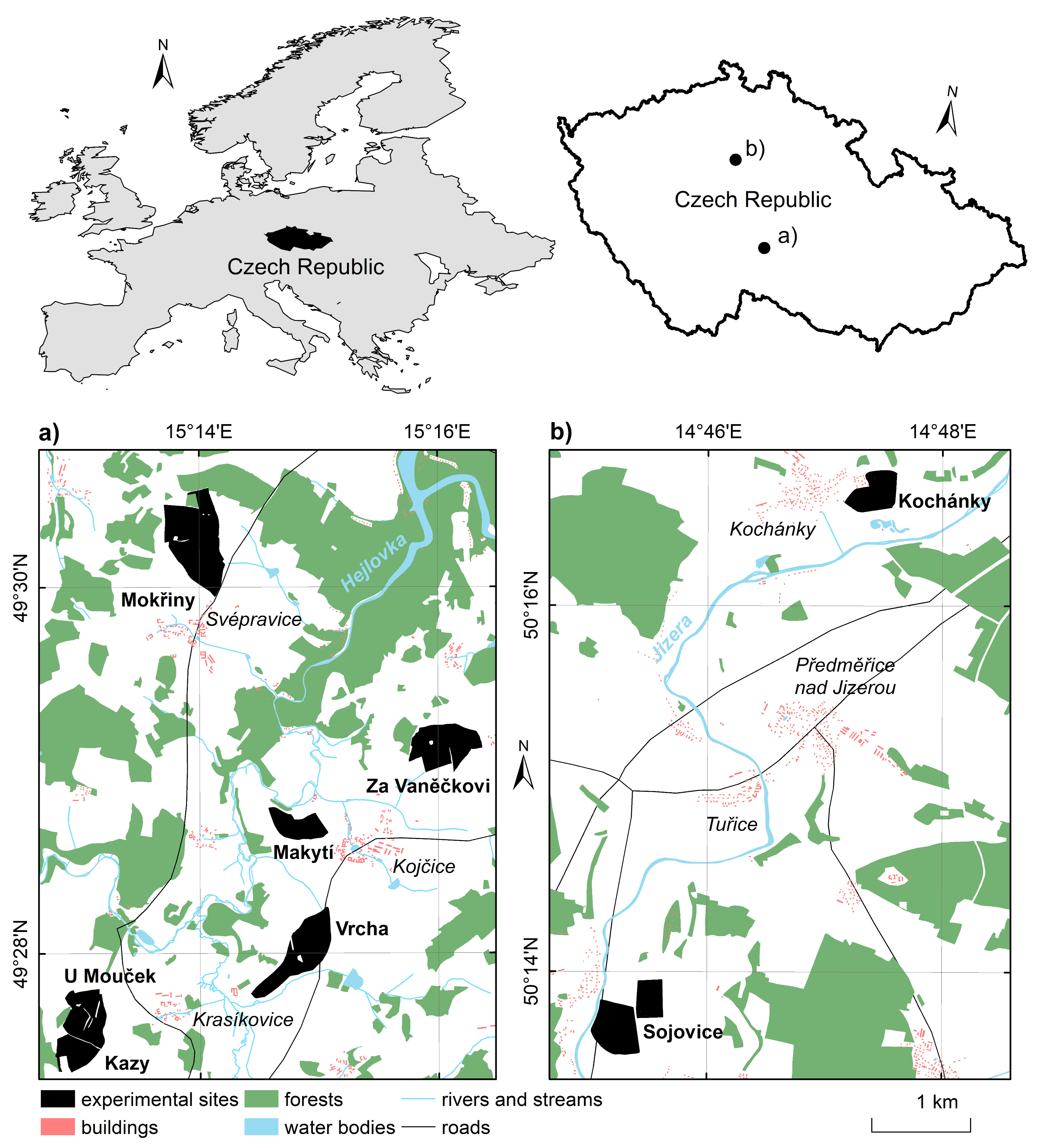
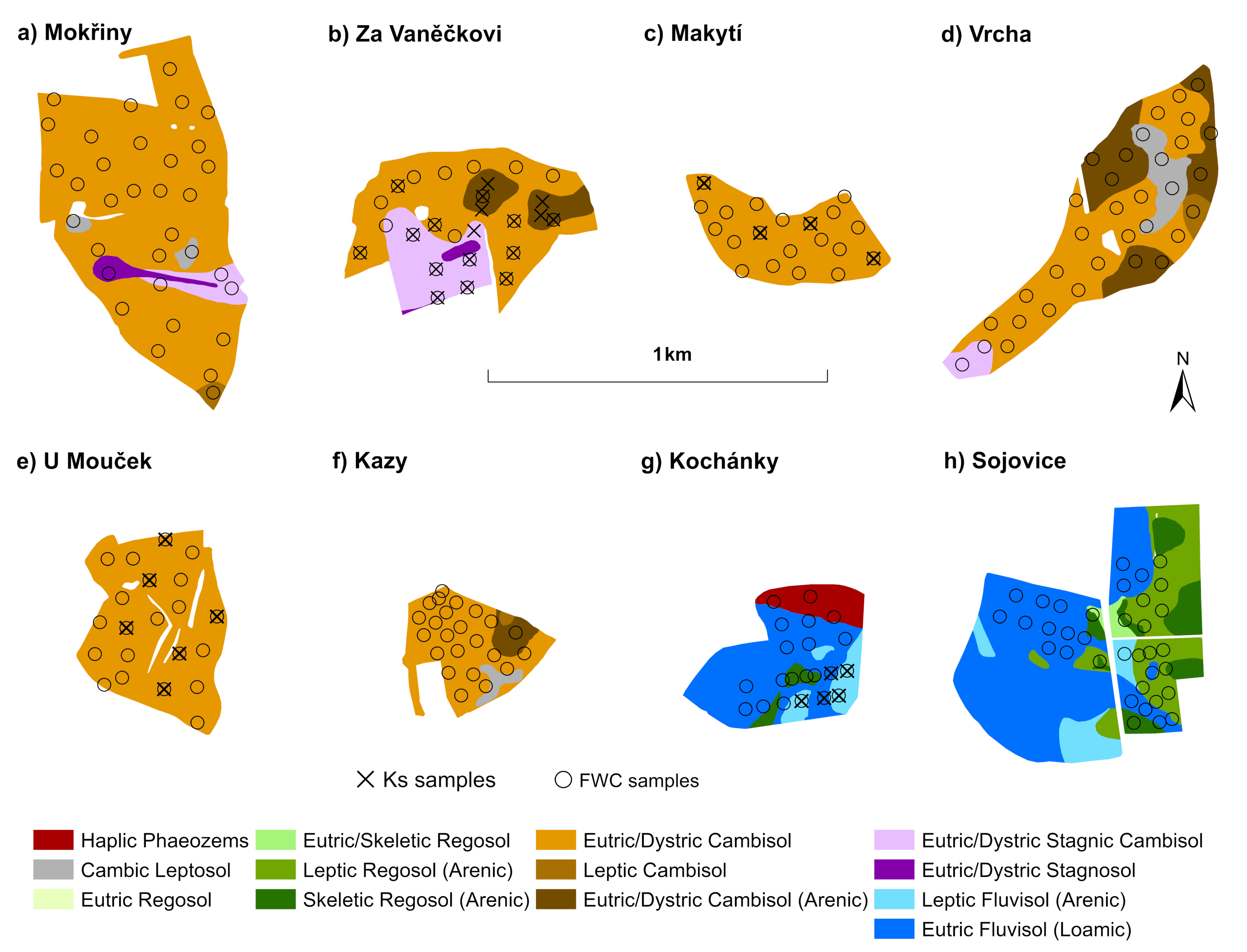
2.1. Study Sites
2.2. Measurements of Saturated Soil Hydraulic Conductivity and Determination of Field Water Capacity
2.3. Remote Sensing Data
2.4. and Estimation from Aerial Data
2.5. Statistical Analysis
3. Results
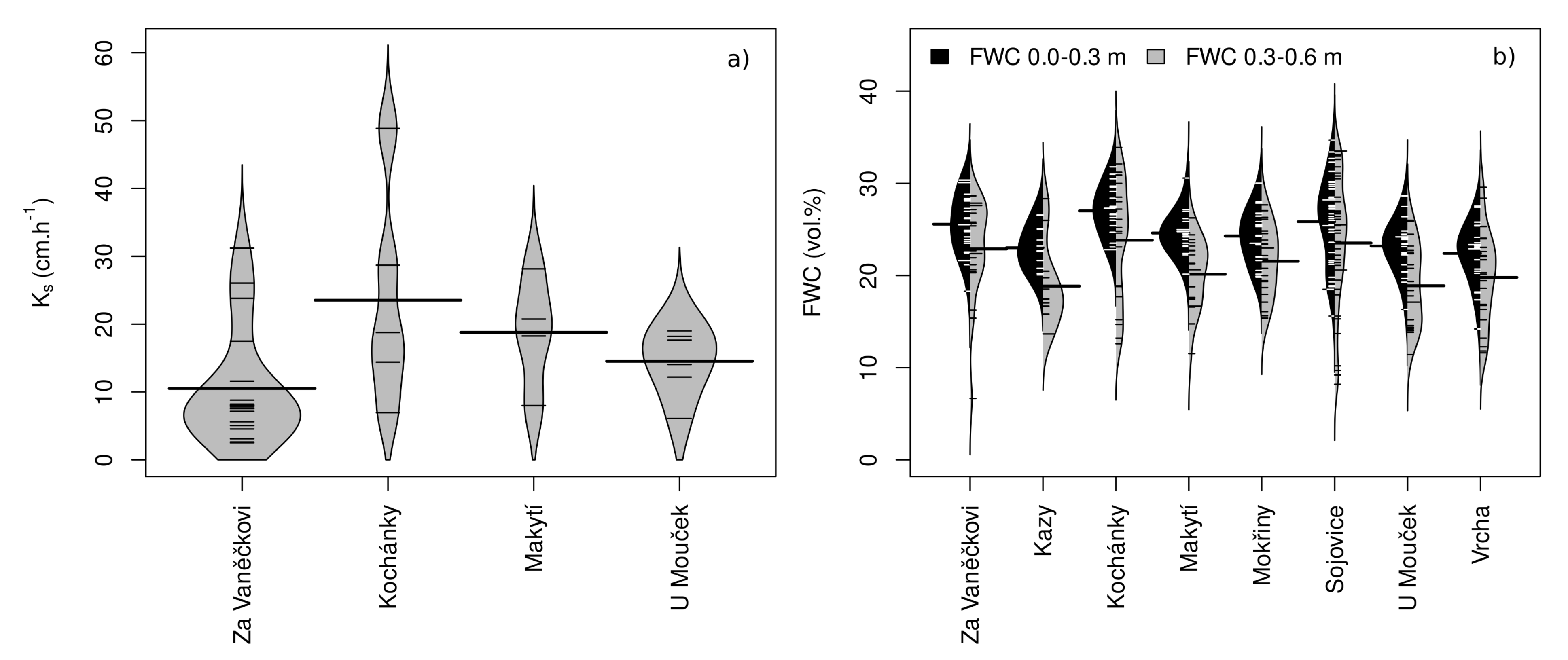
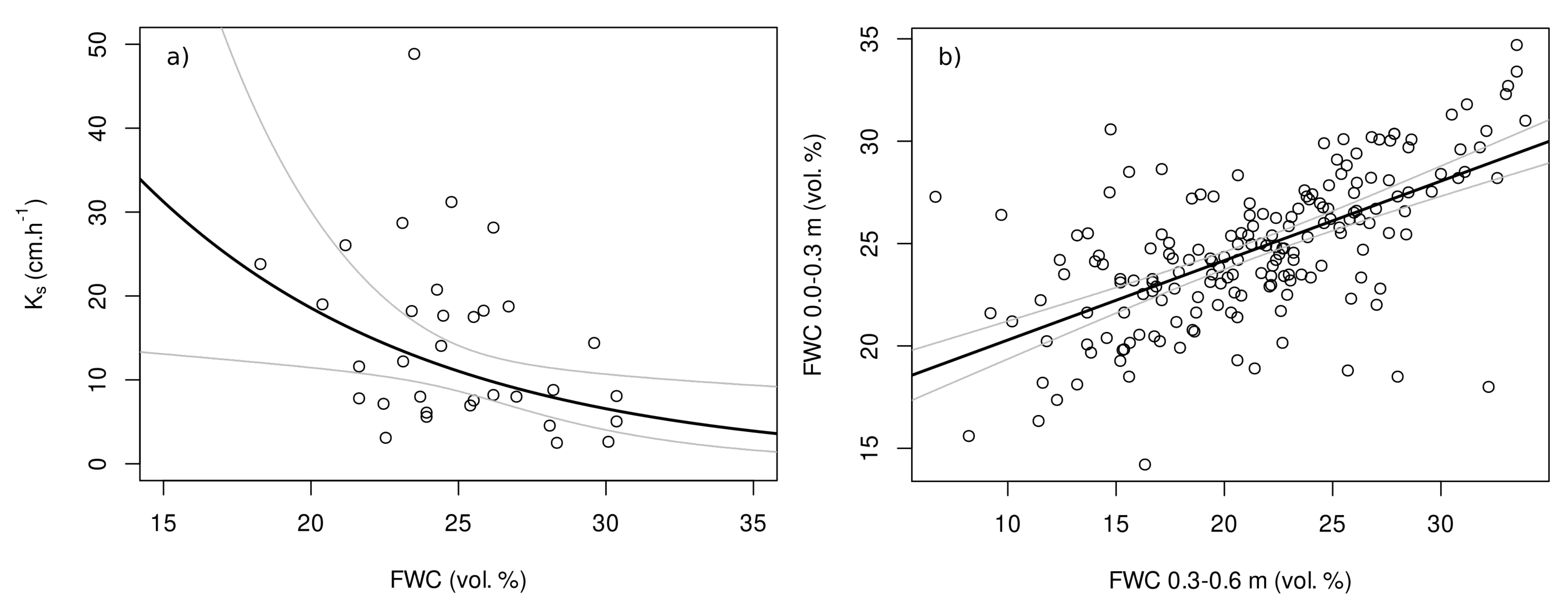
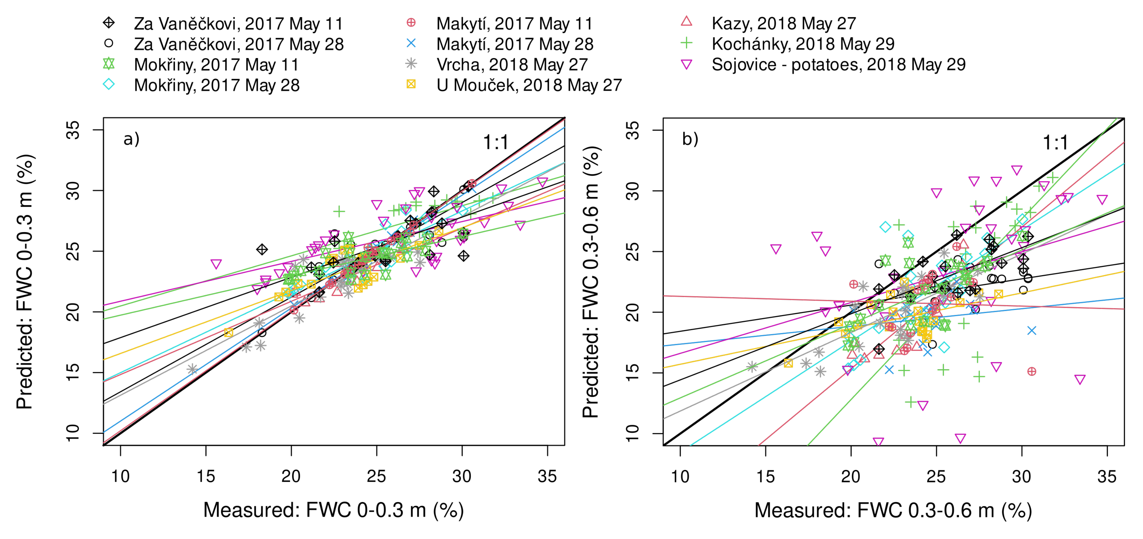
3.1. Measured Data of and
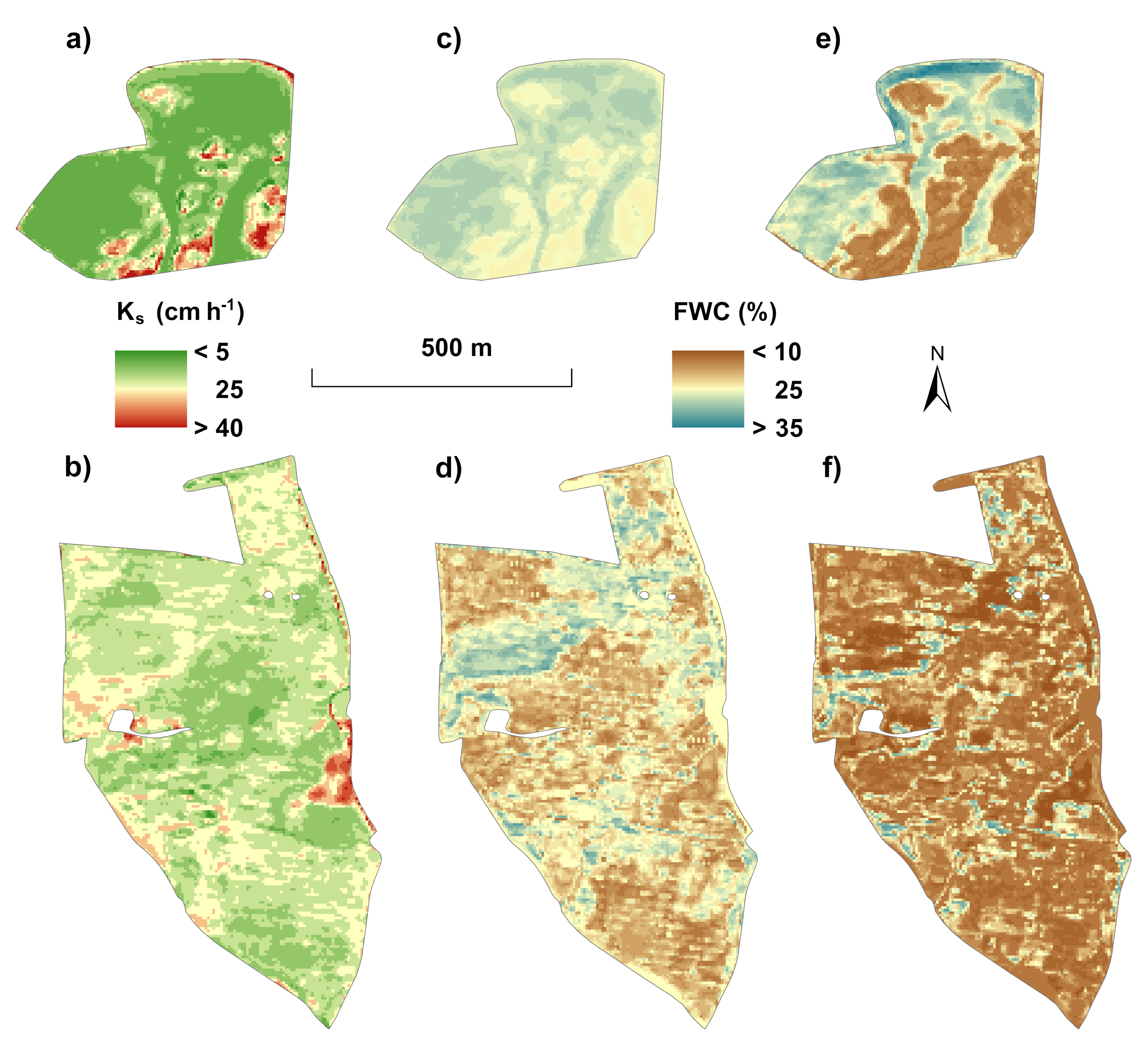
3.2. Estimation of and Data from Aerial Imaging
4. Discussion
4.1. Data and Their Quality
4.2. Estimation of and Data from Aerial Imaging
5. Conclusions
Author Contributions
Funding
Institutional Review Board Statement
Informed Consent Statement
Data Availability Statement
Acknowledgments
Conflicts of Interest
References
- Castellini, M.; Di Prima, S.; Moret-Fernández, D.; Lassabatere, L. Rapid and accurate measurement methods for determining soil hydraulic properties: A review. J. Hydrol. Hydromech. 2021, 69, 121–139. [Google Scholar] [CrossRef]
- Bayabil, H.K.; Dile, Y.T.; Tebebu, T.Y.; Engda, T.A.; Steenhuis, T.S. Evaluating infiltration models and pedotransfer functions: Implications for hydrologic modeling. Geoderma 2019, 338, 159–169. [Google Scholar] [CrossRef]
- Sihag, P.; Tiwari, N.; Ranjan, S. Estimation and inter-comparison of infiltration models. Water Sci. 2017, 31, 34–43. [Google Scholar] [CrossRef]
- Kim, H.; Anderson, S.; Motavalli, P.; Gantzer, C. Compaction effects on soil macropore geometry and related parameters for an arable field. Geoderma 2010, 160, 244–251. [Google Scholar] [CrossRef]
- Shukla, M.K.; Slater, B.K.; Lal, R.; Cepuder, P. Spatial variability of soil properties and potential management classification of a chernozemic field in lower Austria. Soil Sci. 2004, 169, 852–860. [Google Scholar] [CrossRef]
- Jabro, J.D.; Evans, R.G.; Kim, Y.; Iversen, W.M. Estimating in situ soil–water retention and field water capacity in two contrasting soil textures. Irrig. Sci. 2009, 27, 223–229. [Google Scholar] [CrossRef]
- Keller, T.; Sutter, J.A.; Nissen, K.; Rydberg, T. Using field measurement of saturated soil hydraulic conductivity to detect low-yielding zones in three Swedish fields. Soil Tillage Res. 2012, 124, 68–77. [Google Scholar] [CrossRef]
- Van Alphen, B.J.; Stoorvogel, J.J. A Functional approach to soil characterization in support of precision agriculture. Soil Sci. Soc. Am. J. 2000, 64, 1706–1713. [Google Scholar] [CrossRef]
- Usowicz, B.; Lipiec, J. Spatial variability of saturated hydraulic conductivity and its links with other soil properties at the regional scale. Sci. Rep. 2021, 11, 8293. [Google Scholar] [CrossRef]
- Maleki, M.; Mouazen, A.; De Ketelaere, B.; Ramon, H.; De Baerdemaeker, J. On-the-go variable-rate phosphorus fertilisation based on a visible and near-infrared soil sensor. Biosyst. Eng. 2008, 99, 35–46. [Google Scholar] [CrossRef]
- Li, Y.; Shi, Z.; Li, F.; Li, H.Y. Delineation of site-specific management zones using fuzzy clustering analysis in a coastal saline land. Comput. Electron. Agric. 2007, 56, 174–186. [Google Scholar] [CrossRef]
- Koch, B.; Khosla, R.; Frasier, W.M.; Westfall, D.G.; Inman, D. Economic feasibility of variable-rate nitrogen application utilizing site-specific management zones. Agron. J. 2004, 96, 1572–1580. [Google Scholar] [CrossRef]
- Casa, R.; Cavalieri, A.; Lo Cascio, B. Nitrogen fertilisation management in precision agriculture: A preliminary application example on maize. Ital. J. Agron. 2011, 6, 5. [Google Scholar] [CrossRef]
- Kvítek, T.; Žlábek, P.; Bystřický, V.; Fučík, P.; Lexa, M.; Gergel, J.; Novák, P.; Ondr, P. Changes of nitrate concentrations in surface waters influenced by land use in the crystalline complex of the Czech Republic. Phys. Chem. Earth Parts A/B/C 2009, 34, 541–551. [Google Scholar] [CrossRef]
- Doležal, F.; Kvítek, T. The role of recharge zones, discharge zones, springs and tile drainage systems in peneplains of Central European highlands with regard to water quality generation processes. Phys. Chem. Earth Parts A/B/C 2004, 29, 775–785. [Google Scholar] [CrossRef]
- Duffková, R.; Fučík, P.; Jurkovská, L.; Janoušková, M. Experimental evaluation of the potential of arbuscular mycorrhiza to modify nutrient leaching in three arable soils located on one slope. Appl. Soil Ecol. 2019, 143, 116–125. [Google Scholar] [CrossRef]
- Fučík, P.; Zajíček, A.; Duffková, R.; Kvítek, T. Water Quality of Agricultural Drainage Systems in the Czech Republic—Options for Its Improvement; IntechOpen: London, UK, 2015. [Google Scholar] [CrossRef]
- Duffková, R.; Zajíček, A.; Nováková, E. Actual evapotranspiration from partially tile-drained fields as influenced by soil properties, terrain and crop. Soil Water Res. 2011, 6, 131–146. [Google Scholar] [CrossRef]
- Zajíček, A.; Kvítek, T.; Kaplická, M.; Doležal, F.; Kulhavý, Z.; Bystřický, V.; Žlábek, P. Drainage water temperature as a basis for verifying drainage runoff composition on slopes. Hydrol. Process. 2011, 25, 3204–3215. [Google Scholar] [CrossRef]
- Fučík, P.; Zajíček, A.; Kaplická, M.; Duffková, R.; Peterková, J.; Maxová, J.; Takáčová, Š. Incorporating rainfall-runoff events into nitrate-nitrogen and phosphorus load assessments for small tile-drained catchments. Water 2017, 9, 712. [Google Scholar] [CrossRef]
- Fabiani, S.; Vanino, S.; Napoli, R.; Zajíček, A.; Duffková, R.; Evangelou, E.; Nino, P. Assessment of the economic and environmental sustainability of Variable Rate Technology (VRT) application in different wheat intensive European agricultural areas. A Water energy food nexus approach. Environ. Sci. Policy 2020, 114, 366–376. [Google Scholar] [CrossRef]
- Thorup-Kristensen, K.; Halberg, N.; Nicolaisen, M.; Olesen, J.E.; Crews, T.E.; Hinsinger, P.; Kirkegaard, J.; Pierret, A.; Dresbøll, D.B. Digging deeper for agricultural resources, the value of deep rooting. Trends Plant Sci. 2020, 25, 406–417. [Google Scholar] [CrossRef] [PubMed]
- Saxton, K.E.; Rawls, W.J. Soil water characteristic estimates by texture and organic matter for hydrologic solutions. Soil Sci. Soc. Am. J. 2006, 70, 1569–1578. [Google Scholar] [CrossRef]
- Rasoulzadeh, A.; Fatemi, M. Scaling of cumulative infiltration curves using pedotransfer functions. In Proceedings of the 2011 International Conference on New Technology of Agricultural, IEEE, Zibo, China, 27–29 May 2011; pp. 646–650. [Google Scholar] [CrossRef]
- Abdelbaki, A.M.; Youssef, M.A.; Naguib, E.M.F.; Kiwan, M.E.; El-giddawy, E.I. Evaluation of pedotransfer functions for predicting saturated hydraulic conductivity for U.S. soils. In Proceedings of the 2009 Reno, Nevada Conference, Reno, NV, USA, 21–24 June 2009; American Society of Agricultural and Biological Engineers: St. Joseph Charter Township, MI, USA, 2009. [Google Scholar] [CrossRef]
- Novotný, M.; Kervališvili, D.; Šanta, M. Irrigation of Field and Special Crops, 1st ed.; Príroda: Bratislava, Slovakia, 2000. [Google Scholar]
- Haberle, J.; Kurešová, G.; Křížová, K.; Lukáš, J.; Svoboda, P.; Raimanová, I.; Stehlík, M. Maps of spatial variability of soil water capacity. In Hospodaření s Vodou v Krajině; Rožnovský, J., Ed.; Česká Bioklimatologická Společnost: Třeboň, Czech Republic, 2020; p. 14. (In Czech) [Google Scholar]
- Haberle, J.; Duffková, R.; Raimanová, I.; Fučík, P.; Svoboda, P.; Lukas, V.; Kurešová, G. The 13C discrimination of crops identifies soil spatial variability related to water shortage vulnerability. Agronomy 2020, 10, 1691. [Google Scholar] [CrossRef]
- Preza Fontes, G.; Bhattarai, R.; Christianson, L.E.; Pittelkow, C.M. Combining Environmental Monitoring and Remote Sensing Technologies to Evaluate Cropping System Nitrogen Dynamics at the Field-Scale. Front. Sustain. Food Syst. 2019, 3, 8. [Google Scholar] [CrossRef]
- Sigler, W.A.; Ewing, S.A.; Jones, C.A.; Payn, R.A.; Miller, P.; Maneta, M. Water and nitrate loss from dryland agricultural soils is controlled by management, soils, and weather. Agric. Ecosyst. Environ. 2020, 304, 107158. [Google Scholar] [CrossRef]
- Yang, Y.; Zhang, J.; Bao, Z.; Ao, T.; Wang, G.; Wu, H.; Wang, J. Evaluation of multi-source soil moisture datasets over central and eastern agricultural area of China using in situ monitoring network. Remote Sens. 2021, 13, 1175. [Google Scholar] [CrossRef]
- Kornelsen, K.C.; Coulibaly, P. Advances in soil moisture retrieval from synthetic aperture radar and hydrological applications. J. Hydrol. 2013, 476, 460–489. [Google Scholar] [CrossRef]
- Francos, N.; Romano, N.; Nasta, P.; Zeng, Y.; Szabó, B.; Manfreda, S.; Ciraolo, G.; Mészáros, J.; Zhuang, R.; Su, B.; et al. Mapping water infiltration rate using ground and UAV hyperspectral data: A case study of Alento, Italy. Remote Sens. 2021, 13, 2606. [Google Scholar] [CrossRef]
- Wu, D.H.; Fan, W.J.; Cui, Y.K.; Yan, B.Y.; Xu, X.R. Review of monitoring soil water content using hyperspectral remote sensing. Spectrosc. Spectr. Anal. 2010, 30, 3067–3071. [Google Scholar]
- Sobrino, J.; El Kharraz, M. Combining afternoon and morning NOAA satellites for thermal inertia estimation: 2. Methodology and application. J. Geophys. Res. Atmos. 1999, 104, 9455–9465. [Google Scholar] [CrossRef]
- Maltese, A.; Bates, P.; Capodici, F.; Cannarozzo, M.; Ciraolo, G.; La Loggia, G. Critical analysis of thermal inertia approaches for surface soil water content retrieval. Hydrol. Sci. J. 2013, 58, 1144–1161. [Google Scholar] [CrossRef]
- Boulet, G.; Mougenot, B.; Abdelouahab, T.B. An evaporation test based on Thermal Infra Red remote-sensing to select appropriate soil hydraulic properties. J. Hydrol. 2009, 376, 589–598. [Google Scholar] [CrossRef]
- Sadeghi, M.; Babaeian, E.; Tuller, M.; Jones, S.B. The optical trapezoid model: A novel approach to remote sensing of soil moisture applied to Sentinel-2 and Landsat-8 observations. Remote Sens. Environ. 2017, 198, 52–68. [Google Scholar] [CrossRef]
- Ambrosone, M.; Matese, A.; Di Gennaro, S.F.; Gioli, B.; Tudoroiu, M.; Genesio, L.; Miglietta, F.; Baronti, S.; Maienza, A.; Ungaro, F.; et al. Retrieving soil moisture in rainfed and irrigated fields using Sentinel-2 observations and a modified OPTRAM approach. Int. J. Appl. Earth Obs. Geoinf. 2020, 89, 102113. [Google Scholar] [CrossRef]
- Neale, C.M.; Geli, H.M.; Kustas, W.P.; Alfieri, J.G.; Gowda, P.H.; Evett, S.R.; Prueger, J.H.; Hipps, L.E.; Dulaney, W.P.; Chávez, J.L.; et al. Soil water content estimation using a remote sensing based hybrid evapotranspiration modeling approach. Adv. Water Resour. 2012, 50, 152–161. [Google Scholar] [CrossRef]
- Nemani, R.; Pierce, L.; Running, S.; Goward, S. Developing satellite-derived estimates of surface moisture status. J. Appl. Meteorol. Climatol. 1993, 32, 548–557. [Google Scholar] [CrossRef]
- Zhang, D.; Tang, R.; Zhao, W.; Tang, B.; Wu, H.; Shao, K.; Li, Z.L. Surface soil water content estimation from thermal remote sensing based on the temporal variation of land surface temperature. Remote Sens. 2014, 6, 3170–3187. [Google Scholar] [CrossRef]
- Lary, D.J.; Alavi, A.H.; Gandomi, A.H.; Walker, A.L. Machine learning in geosciences and remote sensing. Geosci. Front. 2016, 7, 3–10. [Google Scholar] [CrossRef]
- Xu, C.; Jackson, S.A. Machine learning and complex biological data. Genome Biol. 2019, 20, 76. [Google Scholar] [CrossRef]
- Ahmad, S.; Kalra, A.; Stephen, H. Estimating soil moisture using remote sensing data: A machine learning approach. Adv. Water Resour. 2010, 33, 69–80. [Google Scholar] [CrossRef]
- Ali, I.; Greifeneder, F.; Stamenkovic, J.; Neumann, M.; Notarnicola, C. Review of Machine Learning approaches for biomass and soil moisture retrievals from remote sensing data. Remote Sens. 2015, 7, 16398–16421. [Google Scholar] [CrossRef]
- Cameira, M.; Mota, M. Nitrogen related diffuse pollution from horticulture production—mitigation practices and assessment strategies. Horticulturae 2017, 3, 25. [Google Scholar] [CrossRef]
- Kvítek, T. (Ed.) Retence a Jakost Vody v Povodí vodárenské nádrže Švihov na Želivce: Význam Retence Vody na zeměDělském půdním Fondu Pro Jakost Vody a Současně i průvodce Vodním režimem Krystalinika, 2nd ed.; Povodí Vltavy, State Enterprise, Czech Republic: Prague, Czech Republic, 2018. (In Czech) [Google Scholar]
- Tolasz, R. (Ed.) Climate Atlas of Czechia, 1st ed.; Czech Hydrometeorological Institute, Palacký University Olomouc: Prague, Czech Republic, 2007. (In Czech) [Google Scholar]
- Žigová, A. Development of soils on paragneiss and granite in the southeastern part of Bohemia. Acta Geodyn. Geomater. 2013, 10, 85–95. [Google Scholar] [CrossRef]
- Serrano, S.E. Hydrology for Engineers, Geologists, and Environmental Professionals: An Integrated Treatment of Surface, Subsurface, and Contaminant Hydrology; HydroScience: Lexington, Fayette, 1997. [Google Scholar]
- FAO. World Reference Base for Soil Resources 2014, Update 2015: International Soil Classification System for Naming Soils and Creating Legends for Soil Maps. World Soil Resources Reports No. 106; FAO: Rome, Italy, 2015. [Google Scholar]
- Bruthans, J.; Kůrková, I.; Kadlecová, R. Factors controlling nitrate concentration in space and time in wells distributed along an aquifer/river interface (Káraný, Czechia). Hydrogeol. J. 2019, 27, 195–210. [Google Scholar] [CrossRef]
- Philip, J. Approximate analysis of the borehole permeameter in unsaturated soil. Water Resour. Res. 1985, 21, 1025–1033. [Google Scholar] [CrossRef]
- ISO 11277. Soil Quality–Determination of Particle Size Distribution in Mineral Soil Material–Method by Sieving and Sedimentation; International Organization for Standardization: Geneve, Switzerland, 2009. [Google Scholar]
- Jackson, R.D.; Idso, S.B.; Reginato, R.J.; Pinter, P.J. Canopy temperature as a crop water stress indicator. Water Resour. Res. 1981, 17, 1133. [Google Scholar] [CrossRef]
- Jackson, R.D.; Kustas, W.P.; Choudhury, B.J. A reexamination of the crop water stress index. Irrig. Sci. 1988, 9, 309–317. [Google Scholar] [CrossRef]
- Monin, A.; Obukhov, A. Basic laws of turbulent mixing in the atmosphere near the ground. Tr. Akad. Nauk SSSR Geoph. Inst. 1954, 64, 1963–1987. [Google Scholar]
- Koloskov, G.; Mukhamejanov, K.; Tanton, T. Monin–Obukhov length as a cornerstone of the SEBAL calculations of evapotranspiration. J. Hydrol. 2007, 335, 170–179. [Google Scholar] [CrossRef]
- Monteith, J.L.; Unsworth, M.H. Principles of Environmental Physics, 2nd ed.; Butterworth-Heinemann: Oxford, UK, 1990. [Google Scholar]
- Thom, A.S. Momentum, mass and heat exchange of plant communities. In Vegetation and the Atmosphere, Principles; Monteith, J.L., Ed.; Academic Press: London, UK, 1975; Volume 1, pp. 57–110. [Google Scholar]
- Beljaars, A.C.M.; Holtslag, A.a.M. Flux parameterization over land surfaces for atmospheric models. J. Appl. Meteorol. Climatol. 1991, 30, 327–341. [Google Scholar] [CrossRef]
- Brutsaert, W. Evaporation into the Atmosphere: Theory, History, and Applications; Environmental Fluid Mechanics, Reidel Publishing Company: Dordrecht, The Netherlands; Boston, MA, USA, 1982. [Google Scholar]
- Jarvis, P.; McNaughton, K. Stomatal control of transpiration: Scaling up from leaf to region. In Advances in Ecological Research; Elsevier: Hoboken, NJ, USA, 1986; Volume 15, pp. 1–49. [Google Scholar]
- Qi, J.; Chehbouni, A.; Huete, A.; Kerr, Y.; Sorooshian, S. A modified soil adjusted vegetation index. Remote Sens. Environ. 1994, 48, 119–126. [Google Scholar] [CrossRef]
- Gao, Z.Q.; Liu, C.S.; Gao, W.; Chang, N.B. A coupled remote sensing and the Surface Energy Balance with Topography Algorithm (SEBTA) to estimate actual evapotranspiration over heterogeneous terrain. Hydrol. Earth Syst. Sci. 2011, 15, 119–139. [Google Scholar] [CrossRef]
- Jin, S.; Sader, S. Comparison of time series tasseled cap wetness and the normalized difference moisture index in detecting forest disturbances. Remote Sens. Environ. 2005, 94, 364–372. [Google Scholar] [CrossRef]
- Hatfield, J.L.; Gitelson, A.A.; Schepers, J.S.; Walthall, C.L. Application of Spectral remote sensing for agronomic decisions. Agron. J. 2008, 100, S-117–S-131. [Google Scholar] [CrossRef]
- Peñuelas, J.; Filella, I. Visible and near-infrared reflectance techniques for diagnosing plant physiological status. Trends Plant Sci. 1998, 3, 151–156. [Google Scholar] [CrossRef]
- Jaafar, H.H.; Ahmad, F.A. Time series trends of Landsat-based ET using automated calibration in METRIC and SEBAL: The Bekaa Valley, Lebanon. Remote Sens. Environ. 2020, 238, 111034. [Google Scholar] [CrossRef]
- Huete, A. A soil-adjusted vegetation index (SAVI). Remote Sens. Environ. 1988, 25, 295–309. [Google Scholar] [CrossRef]
- Brom, J. SEBCS for QGIS-Module for Calculation of Energy Balance Features and Vegetation Water Stress Indices. 2021. Available online: https://github.com/JakubBrom/SEBCS (accessed on 20 May 2021).
- Cortes, C.; Vapnik, V. Support-vector networks. Mach. Learn. 1995, 20, 273–297. [Google Scholar] [CrossRef]
- Drucker, H.; Burges, C.J.; Kaufman, L.; Smola, A.; Vapnik, V. Support vector regression machines. Adv. Neural Inf. Process. Syst. 1997, 9, 155–161. [Google Scholar]
- Meyer, D.; Dimitriadou, E.; Hornik, K.; Weingessel, A.; Leisch, F. e1071: Misc Functions of the Department of Statistics, R Package Version 1.7-7; Probability Theory Group (Formerly: E1071), TU Wien; Probability Theory Group: Leiden, The Netherlands, 2021. [Google Scholar]
- R Core Team. R: A Language and Environment for Statistical Computing; R Foundation for Statistical Computing: Vienna, Austria, 2021. [Google Scholar]
- Arrington, K.E.; Ventura, S.J.; Norman, J.M. Predicting saturated hydraulic conductivity for estimating maximum soil infiltration rates. Soil Sci. Soc. Am. J. 2013, 77, 748–758. [Google Scholar] [CrossRef]
- Jadczyszyn, J.; Niedźwiecki, J. Relation of saturated hydraulic conductivity to soil losses. Pol. J. Environ. Stud. 2005, 14, 431–435. [Google Scholar]
- Ahiablame, L.; Chaubey, I.; Smith, D.; Engel, B. Effect of tile effluent on nutrient concentration and retention efficiency in agricultural drainage ditches. Agric. Water Manag. 2011, 98, 1271–1279. [Google Scholar] [CrossRef]
- Kühling, I.; Beiküfner, M.; Vergara, M.; Trautz, D. Effects of adapted N-fertilisation strategies on nitrate leaching and yield performance of arable crops in North-Western Germany. Agronomy 2020, 11, 64. [Google Scholar] [CrossRef]
- Edwards, W.M.; Shipitalo, M.J.; Owens, L.B.; Dick, W.A. Factors affecting preferential flow of water and atrazine through earthworm burrows under continuous no-till corn. J. Environ. Qual. 1993, 22, 453–457. [Google Scholar] [CrossRef]
- Jabro, J.; Stevens, W.B.; Evans, R.G.; Iversen, W.M. Spatial variability and correlation of selected soil properties in the Ap horizon of a CRP grassland. Appl. Eng. Agric. 2010, 26, 419–428. [Google Scholar] [CrossRef]
- Smith, E.A.; Capel, P.D. Specific conductance as a tracer of preferential flow in a subsurface-drained field. Vadose Zone J. 2018, 17, 170206. [Google Scholar] [CrossRef]
- Jabro, J.D.; Stevens, B.W.; Evans, R.G. Spatial relationships among soil physical properties in a grass-alfalfa hay field. Soil Sci. 2006, 171, 719–727. [Google Scholar] [CrossRef][Green Version]
- Zhang, X.X.; Whalley, P.A.; Ashton, R.W.; Evans, J.; Hawkesford, M.J.; Griffiths, S.; Huang, Z.D.; Zhou, H.; Mooney, S.J.; Whalley, W.R. A comparison between water uptake and root length density in winter wheat: Effects of root density and rhizosphere properties. Plant Soil 2020, 451, 345–356. [Google Scholar] [CrossRef] [PubMed]
- Dušek, J.; Vogel, T. Modeling subsurface hillslope runoff dominated by preferential flow: One- vs. two-dimensional approximation. Vadose Zone J. 2014, 13, 1–13. [Google Scholar] [CrossRef]
- Hlaváčiková, H.; Novák, V.; Holko, L. On the role of rock fragments and initial soil water content in the potential subsurface runoff formation. J. Hydrol. Hydromech. 2015, 63, 71–81. [Google Scholar] [CrossRef][Green Version]
- Lin, J.; Govindaraju, R. Conductivity of Soils with Preferential Flow Paths; Technical Report; Kansas State Univ.: Manhattan, KS, USA, 1996. [Google Scholar]
- Němeček, J.; Muhlhanselová, M.; Macků, J.; Vokoun, J.; Vavříček, D.; Novák, P. The Czech Taxonomic Soil Classification System, 2nd ed.; Czech University of Life Science Prague: Prague, Czech Republic, 2011. [Google Scholar]
- Zajíček, A.; Pomije, T.; Kvítek, T. Event water detection in tile drainage runoff using stable isotopes and a water temperature in small agricultural catchment in Bohemian-Moravian Highlands, Czech Republic. Environ. Earth Sci. 2016, 75, 838. [Google Scholar] [CrossRef]
- Kadlecová, R.; Bruthans, J.; Grundloch, J.; Gvoždík, L.; Haberle, J.; Klír, J.; Kůrková, I.; Milický, M.; Růžek, P.; Herčík, L. Kvartérní Sedimenty, Podzemní Voda a Zemědělství; Výzkumný ústav rostlinné výroby, Česká geologická služba, ProGeo, and Pražské vodovody a kanalizace: Prague, Prague, 2018. (In Czech) [Google Scholar]
- Munné-Bosch, S.; Alegre, L. Role of dew on the recovery of water-stressed Melissa officinalis L. plants. J. Plant Physiol. 1999, 154, 759–766. [Google Scholar] [CrossRef]
- Gerlein-Safdi, C.; Koohafkan, M.C.; Chung, M.; Rockwell, F.E.; Thompson, S.; Caylor, K.K. Dew deposition suppresses transpiration and carbon uptake in leaves. Agric. For. Meteorol. 2018, 259, 305–316. [Google Scholar] [CrossRef]
- Vuollekoski, H.; Vogt, M.; Sinclair, V.A.; Duplissy, J.; Järvinen, H.; Kyrö, E.M.; Makkonen, R.; Petäjä, T.; Prisle, N.L.; Räisänen, P.; et al. Estimates of global dew collection potential on artificial surfaces. Hydrol. Earth Syst. Sci. 2015, 19, 601–613. [Google Scholar] [CrossRef]
- Del’Arco Sanches, I.; Feitosa, R.Q.; Achanccaray Diaz, P.M.; Dias Soares, M.; Barreto Luiz, A.J.; Schultz, B.; Pinheiro Maurano, L.E. Campo Verde database: Seeking to improve agricultural remote sensing of tropical areas. IEEE Geosci. Remote Sens. Lett. 2018, 15, 369–373. [Google Scholar] [CrossRef]
- Green, E.P.; Mumby, P.J.; Edwards, A.J.; Clark, C.D. A review of remote sensing for the assessment and management of tropical coastal resources. Coast. Manag. 1996, 24, 1–40. [Google Scholar] [CrossRef]
- Makarieva, A.M.; Gorshkov, V.G. Biotic pump of atmospheric moisture as driver of the hydrological cycle on land. Hydrol. Earth Syst. Sci. 2007, 11, 1013–1033. [Google Scholar] [CrossRef]
- Makarieva, A.M.; Gorshkov, V.G.; Li, B.L. Conservation of water cycle on land via restoration of natural closed-canopy forests: Implications for regional landscape planning. Ecol. Res. 2006, 21, 897–906. [Google Scholar] [CrossRef]
- Makarieva, A.M.; Gorshkov, V.G. The Biotic Pump: Condensation, atmospheric dynamics and climate. Int. J. Water 2010, 5, 365. [Google Scholar] [CrossRef]
- Hesslerová, P.; Pokorný, J.; Brom, J.; Rejšková-Procházková, A. Daily dynamics of radiation surface temperature of different land cover types in a temperate cultural landscape: Consequences for the local climate. Ecol. Eng. 2013, 54, 145–154. [Google Scholar] [CrossRef]
- Huryna, H.; Pokorný, J. The role of water and vegetation in the distribution of solar energy and local climate: A review. Folia Geobot. 2016, 51, 191–208. [Google Scholar] [CrossRef]
- Allen, R.G.; Food and Agriculture Organization of the United Nations (Eds.) Crop Evapotranspiration: Guidelines for Computing Crop Water Requirements; Number 56 in FAO Irrigation and Drainage Paper; Food and Agriculture Organization of the United Nations: Rome, Italy, 1998. [Google Scholar]
- Kroener, E.; Zarebanadkouki, M.; Bittelli, M.; Carminati, A. Simulation of root water uptake under consideration of nonequilibrium dynamics in the rhizosphere: Water content dynamics in the rhizosphere. Water Resour. Res. 2016, 52, 5755–5770. [Google Scholar] [CrossRef]
- Brown, H.; Moot, D.; Pollock, K. Long term growth rates and water extraction patterns of dryland chicory, lucerne and red clover. NZGA: Res. Pract. Ser. 2003, 11, 91–99. [Google Scholar] [CrossRef]
- Haughey, E.; McElwain, J.C.; Finn, J.A. Variability of water supply affected shoot biomass and root depth distribution of four temperate grassland species in monocultures and mixtures. J. Plant Ecol. 2020, 13, 554–562. [Google Scholar] [CrossRef]
- Idso, S.B.; Jackson, R.D.; Reginato, R.J. Remote-sensing of crop yields. Science 1977, 196, 19–25. [Google Scholar] [CrossRef]
- Alderfasi, A.A.; Nielsen, D.C. Use of crop water stress index for monitoring water status and scheduling irrigation in wheat. Agric. Water Manag. 2001, 47, 69–75. [Google Scholar] [CrossRef]
- Irmak, S.; Haman, D.Z.; Bastug, R. Determination of crop water stress index for irrigation timing and yield estimation of corn. Agron. J. 2000, 92, 1221–1227. [Google Scholar] [CrossRef]
- Sepaskhah, A.; Kashefipour, S. Relationships between leaf water potential, CWSI, yield and fruit quality of sweet lime under drip irrigation. Agric. Water Manag. 1994, 25, 13–21. [Google Scholar] [CrossRef]
- Nielsen, D. Scheduling irrigations for soybeans with the crop water stress index (CWSI). Field Crop. Res. 1990, 23, 103–116. [Google Scholar] [CrossRef]
- Gardner, B.R.; Nielsen, D.C.; Shock, C.C. Infrared thermometry and the crop water stress index. I. History, theory, and baselines. J. Prod. Agric. 1992, 5, 462–466. [Google Scholar] [CrossRef]
- Gardner, B.R.; Nielsen, D.C.; Shock, C.C. Infrared thermometry and the crop water stress index. II. Sampling procedures and interpretation. J. Prod. Agric. 1992, 5, 466–475. [Google Scholar] [CrossRef]
- Jones, H.G.; Stoll, M.; Santos, T.; de Sousa, M.; Chaves, M.M.; Grant, O.M. Use of infrared thermography for monitoring stomatal closure in the field: Application to grapevine. J. Exp. Bot. 2002, 53, 2249–2260. [Google Scholar] [CrossRef]
- Jones, H.G.; Serraj, R.; Loveys, B.R.; Xiong, L.; Wheaton, A.; Price, A.H. Thermal infrared imaging of crop canopies for the remote diagnosis and quantification of plant responses to water stress in the field. Funct. Plant Biol. 2009, 36, 978. [Google Scholar] [CrossRef]
- Leinonen, I.; Grant, O.M.; Tagliavia, C.P.P.; Chaves, M.M.; Jones, H.G. Estimating stomatal conductance with thermal imagery. Plant Cell Environ. 2006, 29, 1508–1518. [Google Scholar] [CrossRef]
- Al-Anazi, A.; Gates, I. Support vector regression to predict porosity and permeability: Effect of sample size. Comput. Geosci. 2012, 39, 64–76. [Google Scholar] [CrossRef]
- Babaeian, E.; Sadeghi, M.; Franz, T.E.; Jones, S.; Tuller, M. Mapping soil moisture with the OPtical TRApezoid Model (OPTRAM) based on long-term MODIS observations. Remote Sens. Environ. 2018, 211, 425–440. [Google Scholar] [CrossRef]
- Maltese, A.; Minacapilli, M.; Cammalleri, C.; Ciraolo, G.; D’Asaro, F. A thermal inertia model for soil water content retrieval using thermal and multispectral images. Remote Sens. 2010, 7824, 78241G. [Google Scholar]


| Locality | Soil Type a | Altitude (m a.s.l.) | Area (ha) | Slope (°) | Systematic Drainage (%) | Number of Samples | |
|---|---|---|---|---|---|---|---|
| Za Vaněčkovi | E/DC, E/DSC, E/DCA, E/DS | 569 | 25.3 | 4.2 | 61 | 18 | 26 (21) b |
| Mokřiny | E/DC, LC, E/DSC, E/DS, CL | 578 | 41.4 | 2.3 | <5 | – | 22 |
| Makytí | E/DC | 533 | 12.1 | 3.6 | – | 4 | 20 |
| Vrcha | E/DC, LC, E/DSC, CL, E/DCA | 514 | 26.9 | 4.6 | – | – | 23 |
| U Mouček | E/DC | 544 | 18.5 | 3.8 | – | 6 | 21 |
| Kazy | E/DC, E/DCA, LC, CL, CA, LC | 550 | 10.0 | 2.6 | – | – | 11 |
| Kochánky | LFA, EFL, LRA, SRA, HP | 230 | 15.7 | 1.4 | – | 5 | 21 |
| Sojovice | LFA, EFL, SRA, LRA | 221 | 36.9 | 1.1 | – | – | 35 |
| Locality | Date | Time (UTC) a | No. of Days after Rain > 1 mm | Crop | LAI |
|---|---|---|---|---|---|
| Za Vaněčkovi | 2017 May 11 | 7:15 | 1 | Winter wheat | 2.46 |
| 2017 May 28 | 9:50 | 6 | Winter wheat | 2.91 | |
| Mokřiny | 2017 May 11 | 7:15 | 1 | Winter wheat | 2.73 |
| 2017 May 28 | 9:50 | 6 | Winter wheat | 3.49 | |
| Makytí | 2017 May 11 | 7:15 | 1 | Pea | 0.08 |
| 2017 May 28 | 9:50 | 6 | Pea | 0.50 | |
| Vrcha | 2018 May 27 | 7:10 | 4 | Winter wheat | 2.57 |
| U Mouček | 2018 May 27 | 7:10 | 4 | Mixture for silage | 3.74 |
| Kazy | 2018 May 27 | 7:10 | 4 | Winter wheat | 2.32 |
| Kochánky | 2018 May 29 | 7:30 | 6 | Winter wheat | 3.10 |
| Sojovice | 2018 May 29 | 7:30 | 6 | Potatoes | 3.23 |
| Locality | Date | Crop | R | F | df | p-Level a | RMSE |
|---|---|---|---|---|---|---|---|
| Za Vaněčkovi | 11 May 2017 | Winter wheat | 0.49 | 23.47 | 24 | *** | 2.25 |
| 28 May 2017 | Winter wheat | 0.80 | 98.20 | 24 | *** | 1.41 | |
| Mokřiny | 11May 2017 | Winter wheat | 0.52 | 21.44 | 20 | *** | 2.06 |
| 28 May 2017 | Winter wheat | 0.82 | 91.25 | 20 | *** | 1.25 | |
| Makytí | 11 May 2017 | Pea | 0.99 | 1609.0 | 18 | *** | 0.22 |
| 28 May 2017 | Pea | 0.97 | 498.20 | 18 | *** | 0.40 | |
| Vrcha | 27 May 2018 | Winter wheat | 0.83 | 102.60 | 21 | *** | 1.31 |
| U Mouček | 27 May 2018 | Mixture for silage | 0.38 | 11.45 | 19 | ** | 2.17 |
| Kazy | 27 May 2018 | Winter wheat | 0.78 | 31.06 | 9 | *** | 1.17 |
| Kochánky | 29 May 2018 | Winter wheat | 0.43 | 14.05 | 19 | *** | 2.04 |
| Sojovice | 29 May 2018 | Potatoes | 0.42 | 24.06 | 33 | *** | 3.81 |
| Locality | Date | Crop | R | F | df | p-Level a | RMSE |
|---|---|---|---|---|---|---|---|
| Za Vaněčkovi | 2017 May 11 | Winter wheat | 0.35 | 10.26 | 19 | ** | 4.31 |
| 2017 May 28 | Winter wheat | 0.12 | 2.71 | 19 | n.s. | 4.95 | |
| Mokřiny | 2017 May 11 | Winter wheat | 0.81 | 85.78 | 20 | *** | 1.75 |
| 2017 May 28 | Winter wheat | 0.99 | 1996.0 | 20 | *** | 0.37 | |
| Makytí | 2017 May 11 | Pea | 0.46 | 15.34 | 18 | ** | 2.72 |
| 2017 May 28 | Pea | 0.36 | 10.59 | 18 | ** | 3.64 | |
| Vrcha | 2018 May 27 | Winter wheat | 0.50 | 21.01 | 21 | *** | 3.56 |
| U Mouček | 2018 May 27 | Mixture for silage | 0.36 | 10.59 | 19 | ** | 3.64 |
| Kazy | 2018 May 27 | Winter wheat | 0.81 | 37.19 | 9 | *** | 2.19 |
| Kochánky | 2018 May 29 | Winter wheat | 0.84 | 95.37 | 19 | *** | 2.66 |
| Sojovice | 2018 May 29 | Potatoes | 0.43 | 24.63 | 33 | *** | 5.89 |
Publisher’s Note: MDPI stays neutral with regard to jurisdictional claims in published maps and institutional affiliations. |
© 2021 by the authors. Licensee MDPI, Basel, Switzerland. This article is an open access article distributed under the terms and conditions of the Creative Commons Attribution (CC BY) license (https://creativecommons.org/licenses/by/4.0/).
Share and Cite
Brom, J.; Duffková, R.; Haberle, J.; Zajíček, A.; Nedbal, V.; Bernasová, T.; Křováková, K. Identification of Infiltration Features and Hydraulic Properties of Soils Based on Crop Water Stress Derived from Remotely Sensed Data. Remote Sens. 2021, 13, 4127. https://doi.org/10.3390/rs13204127
Brom J, Duffková R, Haberle J, Zajíček A, Nedbal V, Bernasová T, Křováková K. Identification of Infiltration Features and Hydraulic Properties of Soils Based on Crop Water Stress Derived from Remotely Sensed Data. Remote Sensing. 2021; 13(20):4127. https://doi.org/10.3390/rs13204127
Chicago/Turabian StyleBrom, Jakub, Renata Duffková, Jan Haberle, Antonín Zajíček, Václav Nedbal, Tereza Bernasová, and Kateřina Křováková. 2021. "Identification of Infiltration Features and Hydraulic Properties of Soils Based on Crop Water Stress Derived from Remotely Sensed Data" Remote Sensing 13, no. 20: 4127. https://doi.org/10.3390/rs13204127
APA StyleBrom, J., Duffková, R., Haberle, J., Zajíček, A., Nedbal, V., Bernasová, T., & Křováková, K. (2021). Identification of Infiltration Features and Hydraulic Properties of Soils Based on Crop Water Stress Derived from Remotely Sensed Data. Remote Sensing, 13(20), 4127. https://doi.org/10.3390/rs13204127