Random Forest Regression Model for Estimation of the Growing Stock Volumes in Georgia, USA, Using Dense Landsat Time Series and FIA Dataset

Abstract

The forest volumes are essential as they are directly related to the economic and environmental values of the forests. Satellite-based forest volume estimation was first developed in the 1990s, and the accuracy of the estimation has been improved over time. One of the satellite-based forest volume estimation issues is that it tends to overestimate the large volume class and underestimate the small volume class. Free availability of the major satellite imagery and the development of cloud-based computational platforms facilitate an immense amount of satellite imagery in the estimation. In this paper, we set three objectives: (1) to examine whether the long Landsat time series contributes to the improvement of the estimation accuracy, (2) to explore the effectiveness of forest disturbance record and land cover data as ancillary spatial data on the accuracy of the estimation, and (3) to apply the bias correction method to reduce the bias of the estimation. We computed three Tasseled-cap components from the Landsat data for preparation of short (2014–2016) and long (1984–2016) time series. Each data entity was analyzed with harmonic regressions resulting in the coefficients and the fitted values recorded as pixel values in a multilayer raster database. Data included Forest Inventory and Analysis (FIA) unit field inventory measurements provided by the United States Department of Agriculture Forest Service and the National Land Cover Database and disturbance history data added as ancillary information. The totality of the available data was organized into seven distinct Random Forest (RF) models with different variables compared against each other to identify the ones with the most satisfactory performance. A bias correction method was then applied to all the RF models to examine the effectiveness of the method. Among the seven models, the worst one used the coefficients and fitted values of the short Landsat time series only, and the best one used coefficients and fitted values of both short and long Landsat time series. Using the Out-of-bag (OOB) score, the best model was found to be 34.4% better than the worst one. The model that used only the long time series data had almost the same OOB score as the best model. The results indicate that the use of the long Landsat time series improves model performance. Contrary to the previous research employing forest disturbance data as a feature variable had almost no effect on OOB. The bias correction method reduced the relative size of the bias in the estimates of the best model from 3.79% to −1.47%, the bottom 10% bias by 12.5 points, and the top 10% bias by 9.9 points. Depending on the types of forest, important feature variables were differed, reflecting the relationship between the time series remote sensing data we computed for this research and the forests’ phenological characteristics. The availability of Light Detection And Ranging (LiDAR) data and accessibility of the precise locations of the FIA data are likely to improve the model estimates further.

1. Introduction

Forest densities and volumes are the most important forest attributes used by the forest product industry in forest management and planning. The forest volumes are directly related to the economic benefits of the forest operations, while the forest densities, which directly determine the piece-size of logged timber and associated with it investment returns, are also important elements of various ecosystem functions and wildlife habitats, such as the maximum basal area suitable for the habitat of the red-cockaded woodpecker (Picoides borealis) is suggested to be 18.4 m${}^2$/ha [1]. Furthermore, the timber volume and density are directly related to carbon sequestration [2] and sustainability analysis [3].

In the United States, both private and public organizations manage forest inventories and their measurements. The United States Department of Agriculture (USDA) Forest Service’s Forest Inventory and Analysis (FIA) unit provides access to data from their large-scale, continuous forest inventory. The main objectives of the USDA Forest Service FIA unit are to determine the extent, condition, volume, and growth of forests and the estimation of the changes in their landbase [4]. The inventory splits the conterminous United States into 28,000 constituent hexagons, with their centers approximately 27.4 km apart. The centers of the constituent hexagons serve as the field survey points, with each established FIA plot representing about 2428 hectares. In addition to the central point, three additional satellite sample points are located around the central point of each hexagonal (Figure 1).

All the trees within a plot whose diameter at breast height are greater than 12.7 cm are measured [5]. Although these data provide a good estimation of volume at the state-level, they are not suitable for sub-county-level estimations of the stand volumes. Many public and private landowners conduct separate inventory assessments using ground measurements, forest information systems, and various associated field data. Their inventories may provide higher-resolution volume estimations, but these systems are spatially limited to their individual property boundaries, and as privately owned information, they are generally treated as company assets and are not available publicly.

Satellite-based forest volume estimation was first developed in the 1990s for the purpose of building national-scale forest inventories. This approach combines field inventory data with satellite or other airborne sensor measurements represented by the imagery. Statistical models are applied to estimate the volume for each pixel in the raster database associated with each image. Landsat imagery is the most frequently used type of imagery with k-nearest neighbors (kNN) methods modeling estimated volumes onto the pixels spatially corresponding to the ground measurement locations and propagating the same information onto other spectrally similar pixels. The combination of FIA ground measurements and estimates of volume mapped on the Landsat TM imagery enables us to develop a distribution of forest resources at a pixel-level spatial resolution. The first operational application based on this type of approach was developed in 1990 in Finland [6]. The product derived through this process was a 30 m resolution raster database with the pixel based growing stock volume estimates. Following the Finnish example, a similar inventory was created in Sweden [7,8]. After these successful implementations of the kNN approach to forest inventory spatial estimates in Finland and Sweden, similar approaches were applied in many regions and national forest inventories in the USA, Norway, Ireland, and Japan [9,10,11,12,13]. Recently, Random Forest (RF) algorithm has obtained popularity as another statistical estimation method.

The developments of various methods based on the use of satellite imagery data and the advancements in the satellite sensor technology have led to various new developments of improved kNN-based approaches. In the earlier research involving kNN methods, satellite imagery was used singularly at an individual date posing problems with cloud coverage at given times, which was subsequently addressed by creating composite images spanning over a year [14,15]. Since the release of Landsat imagery to the public domain in October 2008, there has been a marked increase in the quantity of satellite imagery used in research [16,17]. A notable improvement was the use of all available Landsat imagery for the estimations of the land use changes and disturbance tracking [18,19,20]. In this type of research, multiple images acquired within established spatial and temporal boundaries are employed collectively to construct Landsat Time Series (LTS) data, allowing for the tracking of stand changes over time. The time series datasets are usually decomposed trends, seasonal changes, and noise components, prior to the analysis of the land use changes. The raw pixel values of satellite imagery are regarded to be a quasi-systematic reflection of the land surface [20]. The derivatives of the raw pixel values are then used as inputs into the land use change analysis. Although the considerable computational power necessary to analyze all the available satellite imagery has made it more difficult to perform these types of analyses, the rise of cloud-based computational platforms has provided the ability for such large-scale geospatial analyses. Google Earth Engine (GEE), for instance, serves as one of the most prominent platforms for the implementation of large-scale geospatial analyses [21].

Nguyen et al. [22] discuss two major advantages of using LTS: The first advantage is that it extracts the records of the spectral information regarding disturbances and regenerations [23,24,25,26]. Second, it fills spatial and temporal data gaps in the estimation. The incorporation of the forest dynamics is proven to significantly improve the accuracy of the model estimations. Most of the research based on LTS imagery composite suggests choosing the best available pixel from the various annual images in each year [27,28]. This process creates an annual composite of LTS over the time period. Some researchers also suggest creating a composite LTS using more imagery per year than annual or near-annual LTS. The utility of seasonal LTS is explored and found to be able to improve the volume estimation accuracy [29,30,31]. Wilson et al. [32] performed a harmonic regression on all available Landsat imagery and found that the estimations showed a two- to three-fold increase in the explained variance. Wilson et al. [32] thoroughly examined the advantage of using relatively short LTS (2013–2016) and did not inspect the advantage of using the longer LTS.

In the study described in this paper, we set the following three objectives on the forest growing stock volume estimation: (1) to examine whether the long Landsat time series contributes to the improvement of the estimation accuracy, (2) to explore the effectiveness of forest disturbance record and land cover data as ancillary spatial data on the accuracy of the estimation, and (3) to apply the bias correction method to reduce the bias of the estimation. We developed models that estimate the growing stock volume of forests in the state of Georgia, United States, using an RF regression. The models’ accuracy were evaluated by the Out-of-bag (OOB) score and the relative RMSE (rRMSE). The bias of the models was evaluated by the relative bias (rB).

2. Materials and Methods

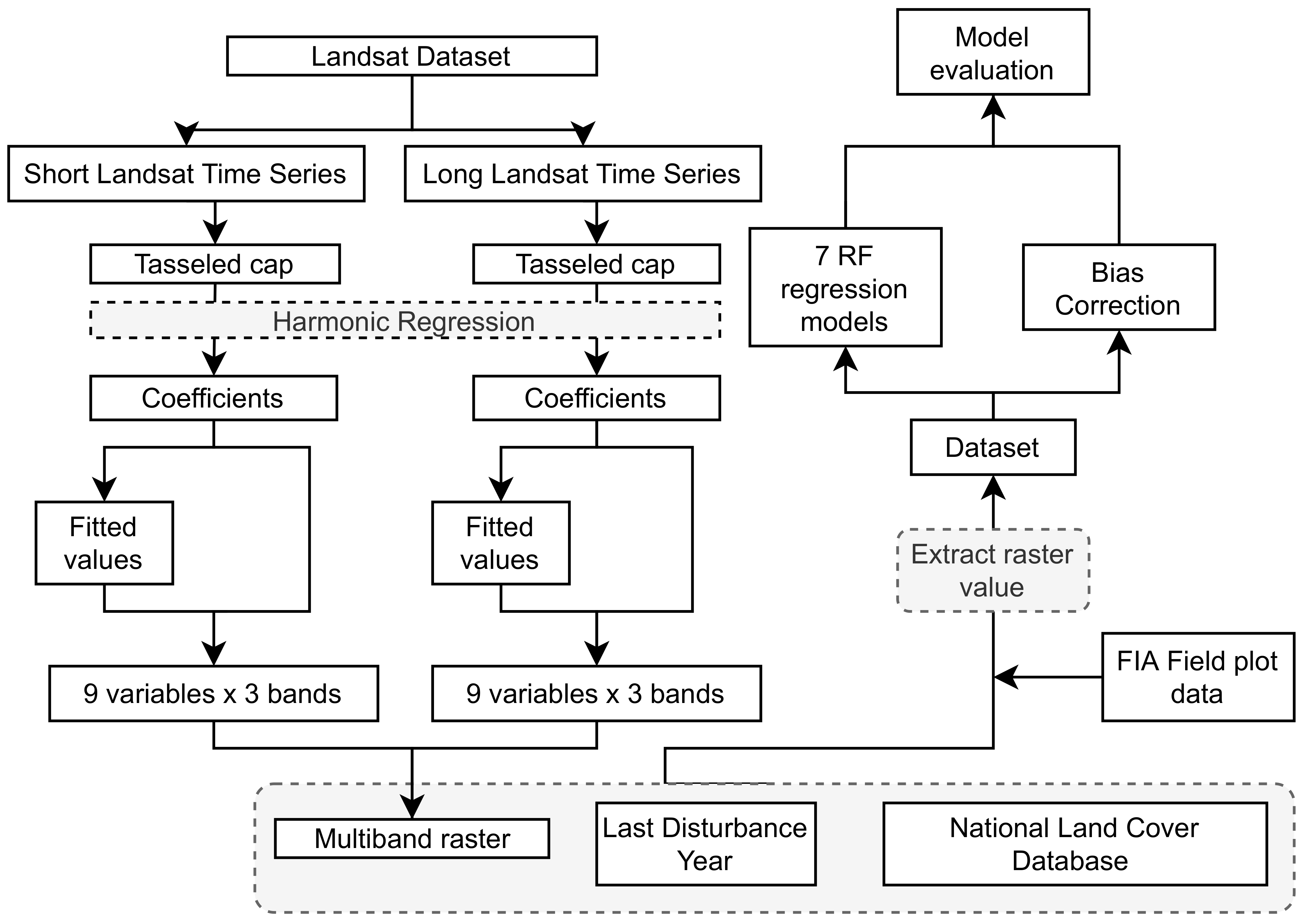
2.1. Research Overview

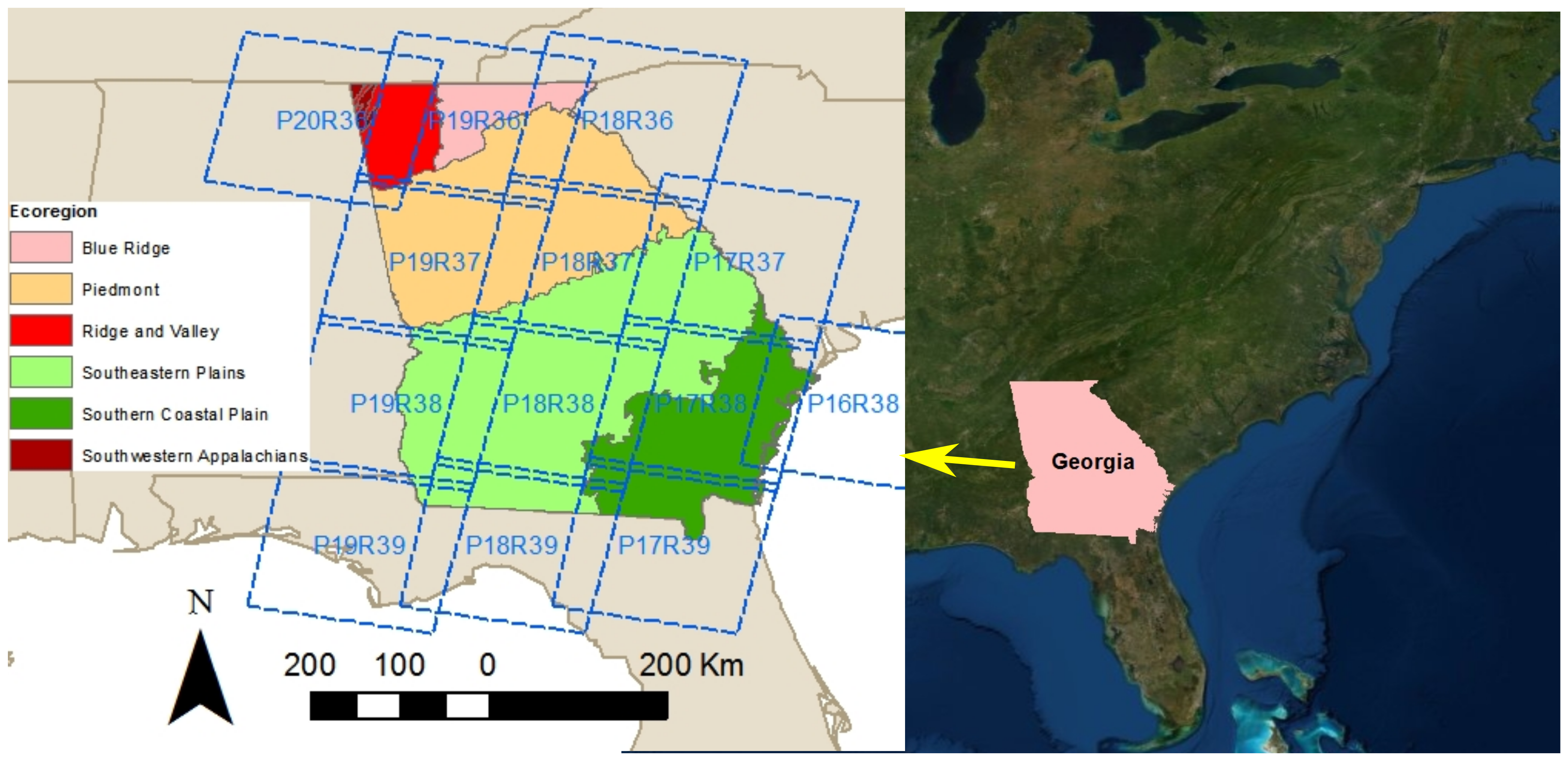
The workflow of this study is illustrated in Figure 2. The following analyses were completed for each objective. For the first objective, we prepared two types of LTS with imagery originating from a distinct time range in each data. Subsequently, we transformed the time series data into Fourier series via harmonic regression. From each series, we retrieved the key values that were used as the feature variables of the RF regression and created a multilayer raster, in which pixel values represent the key values. We combined the publicly available field inventory data with the multilayer raster data to create the tabular data used in the RF regression with various combinations of the feature variables to determine the best combination of them and to test the importance of individual features. For the sake of the second objective, we added two types of ancillary raster data to the combination of the feature variables derived from LTS. The first type of data was raster data, in which the pixel values represent the last disturbance year of the forest stands since 1987. Another ancillary data was land cover data. Next, we examined the contribution of these two ancillary databases to the estimation. For the third objective, we examined the impact of the bias correction model on the predictions when it was applied to the best RF model of all the models we built. Finally, based on the results of the work, we considered the differences between all the various situations and the factors contributing to the improvements of the estimations.

2.2. Study Area

Our study area is the state of Georgia, United States. Georgia is located in the southeastern region of the United States and contains approximately 15 million ha of land area (Figure 3). In the Southern Coastal Plain plantation forests are often intensively managed. The main plantation species is loblolly pine (Pinus taeda), which has a rotation age of 20–25 years under intensive management [33,34]. The Southeastern Plains ecoregion is covered by a mosaic of cropland, pasture, woodland, and forest. The Piedmont ecoregion is located between the Appalachian Mountains and the Southeastern Plains, and it includes the Atlanta metropolitan area, where more than 50% of the Georgia population resides. In the Appalachian mountain area, most of the forests are hardwood or mixed forest that are less frequently disturbed [35].

2.3. Satellite Data

All of the satellite data in this study were queried and processed using the GEE platform. All of the Landsat data were selected from the Level-1 Precision Terrain corrected product (L1TP) for 13 path/row combinations, as shown in Figure 3. The L1TP satisfies both radiometric and geometric criteria set by the United States Geological Survey (USGS) [36]. From the L1TP collection, we selected Landsat 5 TM and Landsat 7 ETM+ Surface Reflectance data, which were generated using the Landsat Ecosystem Disturbance Adaptive Processing System (LEDAPS) algorithm [37].

We compiled two different time ranges to create distinctive LTS. The short range was limited to 3 years and ranged from the beginning of 2014 to the end of 2016. The long range was set to 33 years, spanning from 1984 to 2016. All available images were queried for each time range. For the two sets of images, clouds, cloud shadows, water, and snow interference were masked out using the C Function of Mask (CFMask) algorithm [38,39,40]. For convenience, we refer to the long Landsat time series as the “Long Landsat Time Series” (LLTS) data. Similarly, we call the short Landsat time series as the “Short Landsat Time Series” (SLTS) data. Additionally, we computed the Tasseled Cap Brightness (TCB), Tasseled Cap Greenness (TCG), and Tasseled Cap Wetness (TCW) using surface reflectance data. The coefficients calculated in [41] were applied to compute the TCB, TCG, and TCW. Subsequently, these values were input into a multilayer time series raster. Additionally, an ordinary least squares, harmonic regression was performed to fit the Fourier series to each Tasseled Cap band for both SLTS and LLTS (Figure 4). The form of the Fourier curve is derived from [42] and is as follows,

$$\widehat{Y_t}={\beta }_0+{\beta }_{1}t+{\beta }_{2}cos\left(2\pi \omega t\right)+{\beta }_{3}sin\left(2\pi \omega t\right)$$

(1)

where $\widehat{Y_t}$: Fitted values for the imagery taken at t, ${\beta }_0$: Intercept, ${\beta }_1$: Slope, ${\beta }_2$: Cosine term coefficient, and ${\beta }_3$: Sine term coefficient.

We fixed $\omega =1$ so that the Fourier curve has a single cycle in a year, although there is previous research that assigns $\omega$ a greater value than 1 to obtain multiple cycles in a year [43]. All four coefficients of the Equation (1) are stored as the raster values. The amplitude is computed as follows.

$$amplitude=\sqrt{{\beta }_2^2+{\beta }_3^2}$$

(2)

The impact of the $amplitude$ is on the height of the wave. Fitted values were computed for all the dates for which LTS was acquired. Next, we calculated the maximum, minimum, mean, and RMSE from both the fitted and the observed values (Figure 5). Consequently, 9-band imagery was created for each band by stacking all derived metrics. Then, each of the bands generated from SLTS and LLTS was compiled to create the single raster layer used for the subsequent analysis.

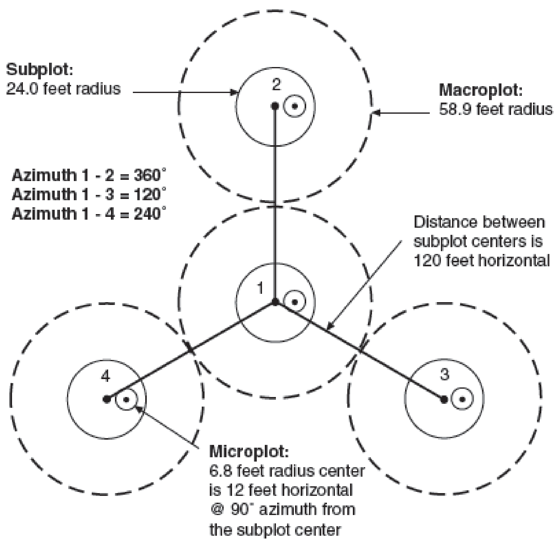
2.4. Ancillary Databases

In addition to the remote sensing data, we used two ancillary databases, which had the potential to help to improve the RF predictions. The first of these was the 2016 National Land Cover Database (NLCD) Land Cover products for the conterminous United States [44]. The Multi-Resolution Land Characteristics consortium created the 2016 NLCD to provide consistent multi-temporal land cover, and land cover change maps for the conterminous United States at 30 m spatial resolution. The 2016 NLCD classifies the land into 16 classes. Out of these 16 classes, the land where shrubs or trees cover more than 20% of the area is classified either as deciduous forest, evergreen forest, mixed forest, or woody wetlands. We note that more than 20% of the FIA field inventory data are positioned on locations where the land cover class is not forested

Table 1. National Land Cover Database (NLCD) 2016 Land Cover Class on the FIA field plots.

Land Cover Class	Class ${}^1$	# of Plots	Mean Volume (m${}^3$/ha)	# of Plots Disturbed ${}^2$
Water	0	4	220.61	2
Developed	0	43	330.14	6
Barren land	0	2	146.99	1
Deciduous forest ${}^{3,4}$	2	191	433.5	21
Evergreen forest ${}^{3,4}$	1	274	431.61	80
Mixed forest ${}^{3,4}$	2	75	416.8	10
Shrubland	0	32	138.43	16
Herbaceous	0	28	148.46	19
Planted/Cultivated	0	51	132.47	2
Woody wetlands ${}^3$	2	185	462.28	32

¹ 0: Non-forest. 1: Evergreen Forest. 2: Non-Evergreen. ² Disturbance record for each plot was retrieved from [45]. ³ Areas where forest or shrubland vegetation accounts for greater than 20% of vegetative cover. ⁴ Areas dominated by trees generally greater than 5 m tall.

. We included all field inventory data that is classified as non-forest in a later analysis, as the NLCD misclassifies some of the forest pixels as a non-forest class. The second ancillary database used in this research was the last disturbance year map of Georgia. This map depicts the most recent disturbance that occurred between 1984 and 2016 for every land area in the entire state of Georgia at 30 m spatial resolution [45]. Regardless of the current land use, a pixel without any disturbance record between 1984 and 2016 is classified as undisturbed.

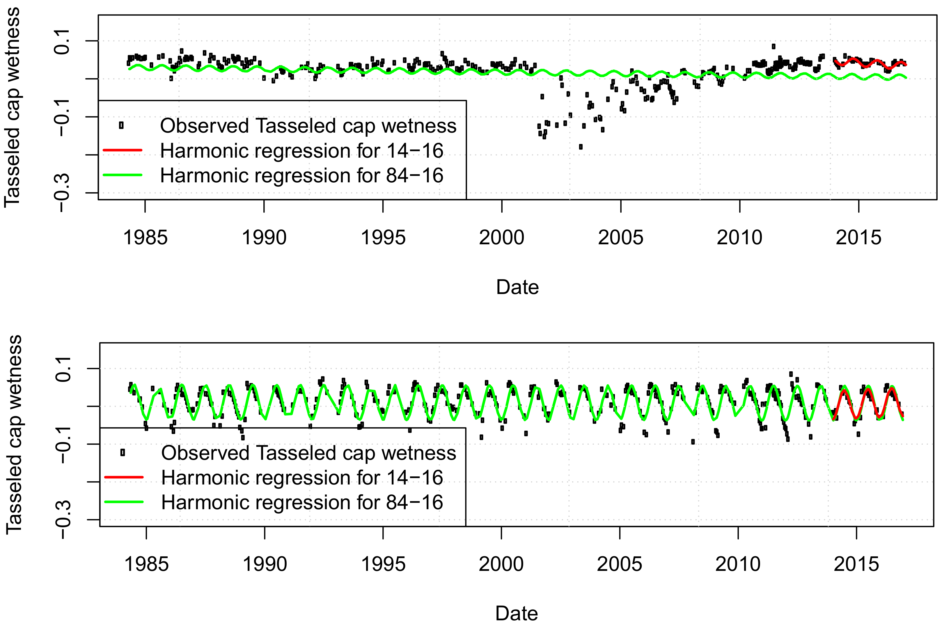
2.5. Growing Stock Estimation

We used the FIA dataset as our ground inventory measurements. Satellite data and ancillary data were stacked into a multilayer raster that contained 56 bands (54 bands from satellite data and two bands from ancillary data). To integrate the raster and the FIA inventory ground measurements data, we requested the USDA Forest Service to extract the pixel values of the raster data onto the field plot points; they extracted our raster data onto the point data and provided us with tabular data containing plot ID numbers and the pixel values of our raster data. We note that all information potentially allowing the data user to detect the exact coordinate of the plot data was removed by USDA Forest Service in compliance with the Privacy Act in 1974 [46]. Thus, we do not know the exact locations of the plots.

The tabular data were aggregated with the FIA’s original database available from the FIA DataMart (https://apps.fs.usda.gov/fia/datamart/datamart.html). The individual tree measurement data were available for each plot ID. Although individual tree measurements are available from the four subplots shown in Figure 1, only the data from the central subplot of a plot were used for the volume calculation, in order to avert the problem of spatial correlation among subplot observations [10]. Based on the code found in [47], individual tree data were aggregated into the plot-level growing stock volume per acre as follows,

$$V_i=\left(\sum _{j=1}^{m_i}{v}_{ij}\right)\times k$$

(3)

where $V_i$: Per hectare growing stock volume of plot i, $v_{ij}$: Net m${}^3$ volume of jth tree in plot i equivalent to the net volume of wood in the central stem, $m_i$: The number of trees in plot i, and k: Expansion factor to convert the total growing stock volume of the plot to per hectare growing stock volume. The distribution of the volume for each plot is illustrated in Figure 6.

RF is an algorithm that handles large volumes of data within a relatively short computation time [48]. RF regression is widely used for making data-based predictions, including forest attribute estimation [32,49,50]. One of the primary advantages of using an RF model is that it can determine the importance of a variable, which indicates the contribution of each feature variable to the model prediction. The mean reduction in prediction accuracy evaluates the importance. One of the known issues of RF involves a potential bias in the model predictions. Breiman [51] argues that bagging could diminish the extent of the variance of regression predictors, yet it does not reduce the magnitude of the bias. On the other hand, because extreme observations are estimated using the average of the estimation of each tree, large observations close to the maximum value within the data are underestimated and small values of the regression function are overestimated [52]. When data are imbalanced, estimations using the RF algorithm are more susceptible to the risk of bias [53]. Zhang and Lu [52] propose a method to correct the bias in RF.

For the RF regression, the data were split into the dependent variable, which is the growing stock volume per hectare, and the independent variables that are all derived from Landsat imagery and ancillary data. We calculated the $rRMSE$, the relative bias (rB), and the OOB score. $RMSE$ has been used as the primary determinant of the model performance [54]. As the absolute value of the RMSE is incomparable between research conducted in different study areas, the $rRMSE$, calculated by the following formula, is used in favor of the $RMSE$.

$$rRMSE=\frac{RMSE}{\overline{y}}\times 100$$

(4)

Knowledge of the bias is required to know the direction of the error. Subsequently, rB is calculated in the same way as rRMSE; they are formulated as follows.

$$Bias=\frac{{\displaystyle \sum _{n_i=1}}(y_i-\widehat{y_i})}{n}$$

(5)

$$rB=\frac{Bias}{\widehat{y}}\times 100$$

(6)

In addition to the evaluation of the entire data, we focused on the smallest and largest volume group as it is known that the error of the nonparametric estimation of the volume is usually heteroskedastic [55]. We grouped the field inventory data into deciles based on the observed growing stock volume. The bottom 10% ranged between 0.1 m${}^3$/ha to 12.9 m${}^3$/ha, while the top 10% group ranged between 249.1 m${}^3$/ha to 682.1 m${}^3$/ha. We calculated the bias for the bottom 10%, middle 80%, and top 10%, separately. The RF regressor was trained using the training data. Scikit-learn, a Python module that provides machine learning algorithms for medium-scale supervised and unsupervised problems, was used to perform the RF regression [56]. The number of decision trees created in the RF algorithm was set to 500. The mean squared error was selected as the function to measure the quality of a split in the individual decision trees. Individual decision trees were trained by the data bootstrapped from the original training data.

First, we built a base model that used the coefficients of the harmonic regression on SLTS, LLTS and the last disturbance year record as the feature variables ($C_{SL}$ in

Table 2. Summary of the feature variables.

	Vegetation Index /Data Source	Time Range	# of Variables	Values	RF Models
					${\mathit{C}}_{\mathit{SL}}$	${\mathit{F}}_{\mathit{SL}}$	${\mathit{CF}}_{\mathit{S}}$	${\mathit{CF}}_{\mathit{L}}$	${\mathit{CF}}_{\mathit{SL}}$	${\mathit{E}}_{\mathit{SL}}$	${\mathit{NE}}_{\mathit{SL}}$
Features	Landsat TCB	1984–2016	4	Regression coefficients		✓			✓	✓	✓
		1984–2016	5	Fitted values				✓	✓	✓	✓
		2014–2016	4	Regression coefficients	✓	✓			✓	✓	✓
		2014–2016	5	Fitted values			✓	✓	✓	✓	✓
	Landsat TCG	1984–2016	4	Regression coefficients		✓			✓	✓	✓
		1984–2016	5	Fitted values				✓	✓	✓	✓
		2014–2016	4	Regression coefficients	✓	✓			✓	✓	✓
		2014–2016	5	Fitted values			✓	✓	✓	✓	✓
	Landsat TCW	1984–2016	4	Regression coefficients		✓			✓	✓	✓
		1984–2016	5	Fitted values				✓	✓	✓	✓
		2014–2016	4	Regression coefficients	✓	✓			✓	✓	✓
		2014–2016	5	Fitted values			✓	✓	✓	✓	✓
	NLCD	2016	1	Land use class						✓	✓
	Last disturbance	1984–2016	1	Disturbance year	✓	✓	✓	✓	✓	✓	✓
Response	FIA dataset	2016	1	Growing stock volume	✓	✓	✓	✓	✓	✓	✓
			57 variables		14	26	17	32	56	57	57

). Next, the fitted values of SLTS, LLTS, and the last disturbance year data were selected as the feature variables of the second model ($F_{SL}$ in Table 2). In the third model, we selected both the fitted values and the coefficients of SLTS and the last disturbance year data ($C{F}_S$ in Table 2). To make a comparison with the third model, the fourth model included both the fitted values and the coefficients of LLTS, along with the last disturbance year data ($C{F}_L$ in Table 2). $C{F}_{SL}$, meanwhile, used all of the feature variables from the previous models ($C{F}_{SL}$ in Table 2). After determining the best combination of the variables, as derived from the remote sensing data, we divided the data by the forest type, as defined in the 2016 NLCD. The first group contained only the evergreen forest and was denoted as the Evergreen data. The second group contained the remaining forest groups listed in Table 1 and was denoted as the Non-Evergreen data. Then, the RF model was trained and evaluated separately ($E_{SL}$ and $N{E}_{SL}$ in Table 2). Following this, predictions for each data were aggregated to compute the OOB score and rRMSE as the eighth model ($E_{SL}$ + $N{E}_{SL}$ in

Table 3. Summary of the RF models.

	${\mathit{C}}_{\mathit{SL}}$	${\mathit{F}}_{\mathit{SL}}$	${\mathit{CF}}_{\mathit{S}}$	${\mathit{CF}}_{\mathit{L}}$	${\mathit{CF}}_{\mathit{SL}}$	${\mathit{E}}_{\mathit{SL}}$	${\mathit{NE}}_{\mathit{SL}}$	${\mathit{E}}_{\mathit{SL}}$ + NE${}_{\mathit{SL}}$
Observation Mean	121.21	121.21	121.21	121.21	121.21	113.39	128.16	-
rRMSE	68.93	67.38	71.48	65.09	64.42	59.66	70.50	65.67
rB	4.19	3.48	3.72	2.66	3.79	3.09	4.82	-
OOB_score	34.8	35.87	23.39	35.63	36.11	46.52	34	39.15
Species	all	all	all	all	all	Evergreen	non-Evergreen	all

). To compare OOB between models, we calculated the rate of change as follows,

$$ROC(\%)=\frac{B-A}{A}\times 100$$

(7)

where ROC: rate of change; A: rRMSE, OOB, or rB in model A; and B: rRMSE, OOB, or rB in model B. Percentage point (% point) was used to compare rRMSE and rB.

The bias correction method proposed in [52] was applied to each model to reduce the bias observed in the top and bottom 10% of the volume classes. In the model, we conjectured that bias would be attributed to the response variables. To inspect the effect of the bias correction, the data was split into training and test data, respectively. The ratio of the training to test data was then set to a 2:1 ratio. We created the RF model for the training data and computed the residual of the RF regression (e) as follows,

$$e=Y-\widehat{f}\left(\mathbf{X}\right)-B\left(Y\right)+ϵ$$

(8)

where Y: The growing stock volume of the observations in the training data, $f\left(\mathbf{X}\right)$: Predicted values of the RF regression using feature variables of the training data, $B\left(Y\right)$: Regression bias, and $ϵ$: The error term. $ϵ\sim N(0,{\sigma }^2)$.

$$\widehat{B}\left(Y\right)=\alpha +{\beta }_1{Y}^2+{\beta }_{2}Y$$

(9)

The bias-corrected prediction (${\widehat{f}}_{bc}$) was calculated by subtracting the estimated bias.

$${\widehat{f}}_{bc}=\widehat{f}-\widehat{B}\left(Y\right)$$

(10)

The effect of the correction was evaluated for the test data.

3. Results

We have trained and evaluated the eight models described in the previous section (Table 3). Among the models using all species for the field inventory data, in terms of the OOB score, the best model was $C{F}_{SL}$. This result, when compared to the OOB score of $C{F}_S$, was found to be 35.2% better. The OOB score of $F_{SL}$ was found to be better than $C_{SL}$ by 2.2%. rRMSE of $F_{SL}$ was 1.6% points better than $C_{SL}$. Between the models that used both coefficients and fitted values, $C{F}_L$ showed a better result than $C{F}_S$. The rRMSE of $C{F}_L$ was improved by 6.4% points, while the OOB score was improved by 34.4%. Figure 7 shows the feature importance of the top 10 variables in $C{F}_{SL}$. The maximum value of the TCW generated from SLTS had the highest feature importance. $E_{SL}$ and $N{E}_{SL}$ were trained for the smaller sample sizes, as the data were split based on the forest type. The evergreen forest had a better OOB score than $C{F}_{SL}$ by 9%, whereas $N{E}_{SL}$, which takes field inventory data from non-evergreen samples, returned a lower OOB score than $C{F}_{SL}$. The OOB predictions of $E_{SL}$ and $N{E}_{SL}$ were aggregated to compute the rRMSE and OOB score for the entire data ($E_{SL}$ + $N{E}_{SL}$ in Table 3). The rRMSE for the aggregated prediction was similar to that of $C{F}_{SL}$, while the OOB score for the aggregated prediction was worse than that of $C{F}_{SL}$. The feature importance of $E_{SL}$ and $N{E}_{SL}$ was presented in Figure 7. For evergreen forests, the six most important features were either the TCW or the TCB of LLTS. For the rest of the species, the maximum fitted values of the harmonic regression derived from the TCW of SLTS. The second important feature was the maximum fitted values of the harmonic regression on the TCW of LLTS. In comparison with $E_{SL}$ and $N{E}_{SL}$, the maximum fitted values are given greater importance in $E_{SL}$ than in $N{E}_{SL}$.

The inclusion of LLTS into the set of feature variables was effective. This result coincides with the result shown in previous research [57]. As is shown in the comparison between $C{F}_S$ and $C{F}_L$, the inclusion of LLTS into the set of feature variables contributed to improving the OOB score.

Table 4. Number of top 10 feature variables for $C{F}_{SL}$, $E_{SL}$, and $N{E}_{SL}$.

Length	Model	Max	Mean	Min	RMSE	Sin	Slope	Intercept	Total
SLTS	$C{F}_{SL}$	1	-	-	2	-	-	-	3
	$E_{SL}$	-	1	-	-	-	1	-	2
	$N{E}_{SL}$	1	-	1	-	2	-	-	4
LLTS	$C{F}_{SL}$	1	1	-	2	1	1	1	7
	$E_{SL}$	1	2	1	2	-	-	2	8
	$N{E}_{SL}$	1	1	-	2	1	1	-	6

shows how many times a variable was selected as being one of the 10 most important variables in terms of feature importance for $C{F}_{SL}$, $E_{SL}$, and $N{E}_{SL}$. The number of features created from LLTS is more than SLTS in $C{F}_{SL}$, $E_{SL}$, and $N{E}_{SL}$. In $E_{SL}$, features derived from LLTS were more important than in the $N{E}_{SL}$ model. On the other hand, SLTS maintains a degree of importance for the $N{E}_{SL}$ model. The different effects of LLTS and SLTS on the two models resulting from the different ratios of the field inventory data with disturbance (Table 1). While 29% of the field inventory data of evergreen forest has a disturbance record, only 14% of the field inventory data of the non-Evergreen forest has a disturbance record. As LLTS convolutes the time series trajectory of Landsat spectral values over long periods of time, features from LLTS gained importance in $E_{SL}$, of which field inventory data was taken from the relatively dynamic and young forest. As SLTS captures recent trends more precisely than LLTS, SLTS gained a degree of importance for $N{E}_{SL}$, of which field plot data relate to the relatively stable and mature forest.

The bias correction method was applied to each model. The relationship between the observed growing stock volume and the estimated bias for $C{F}_{SL}$ is illustrated in Figure 8. For each RF model, we subtracted the estimated bias from predicted volumes to acquire the bias-corrected prediction. Bias-corrected prediction reduced rB, bottom 10% bias, and top 10% bias from the original prediction in all models (

Table 5. Summary of the relative bias for each volume group. rB: relative bias, rB_corr: relative bias with bias correction, middle80: relative bias of the middle 80% volume class, middle80: relative bias of the middle 80% volume class with bias correction, bottom10: relative bias of the bottom 10% volume class, bottom10_corr: relative bias of the bottom 10% volume class after bias correction, top10: relative bias of the top 10% volume class, and top10_corr: relative bias of the top 10% volume class with bias correction.

	${\mathit{C}}_{\mathit{SL}}$	${\mathit{F}}_{\mathit{SL}}$	${\mathit{CF}}_{\mathit{S}}$	${\mathit{CF}}_{\mathit{L}}$	${\mathit{CF}}_{\mathit{SL}}$	${\mathit{E}}_{\mathit{SL}}$	${\mathit{NE}}_{\mathit{SL}}$
rB	4.19	3.48	3.72	2.66	3.79	3.09	4.82
rB_corr	−2.73	−1.98	−1.48	−0.69	−1.47	−1.26	−2.86
middle80	−16.63	−15.42	−16.19	−11.94	−14.1	−15.17	−15.857
middle80_corr	−14.41	−13.08	−13.6	−9.01	−10.91	−12.61	−13.23
bottom10	−69.16	−65.42	−71.37	−71.51	−69.89	−53.39	−71.03
bottom10_corr	−56.43	−52.74	−58.14	−60.13	−57.43	−42.03	−56.31
top10	151.93	146.08	159.81	138.88	140.93	141.87	142.24
top10_corr	139.55	132.90	152.97	127.93	131.01	128.26	128.88

).

4. Discussion

We constructed multiple models and evaluated them in the previous section for the three objectives. Regarding the first objective, comparison between $C{F}_S$ and $C{F}_L$ contrasted the effect of the length of LTS as the difference between these models is only the length of LTS employed as the feature variables. $C{F}_L$ showed 34.4% better OOB than $C{F}_S$ that it is reasonable to conclude that using LLTS as feature variables contributes to the improvement of the estimation accuracy. In addition, $C{F}_L$ reduced the bias of the top 10% volume class by 21% points from $C{F}_S$. This difference might be caused by the characteristics of feature variables derived from LLTS that are less likely to spectrally saturate. The saturation of the spectral reflectance value of satellite imagery refers to the situation whereby spectral reflectance values mimic the values normally seen in forest vegetation with dense canopy cover. This phenomenon is the decisive factor in the low estimation accuracy of the forest aboveground biomass and volume estimation, especially when the volume or aboveground biomass is high [58,59]. The second objective was examined by focusing on disturbance year and NLCD data. In any model that used disturbance year and NLCD data as feature variables, these variables did not have importance more than 0.02. This fact indicates that the contribution of two ancillary spatial data was less important than LTS. The difference between the OOB score of the model without the disturbance year record and the model with the disturbance year record was less than 0.01, unlike the previous research that showed the importance of the disturbance metrics on the model performance [23,24,25]. The plausible reason for the relative unimportance of the last disturbance year’s data is that 80% of our field inventory data does not have any disturbance records. To make the information about the dynamics of the forest stands more relevant to the changes, combining more metrics acquired from the change detection algorithms (i.e., magnitude of disturbance and start of regeneration) is necessary. Effectiveness of NLCD was examined by the comparison between $C{F}_{SL}$ and aggregated model of $E_{SL}$ and $N{E}_{SL}$ ($E_{SL}+N{E}_{SL}$ in Table 3) as $E_{SL}+N{E}_{SL}$ is constructed by adding only NLCD land cover class to the feature variables (Table 2). While the OOB socre of $E_{SL}+N{E}_{SL}$ was better than $C{F}_{SL}$, rRMSE of $E_{SL}+N{E}_{SL}$ was slightly worse than $C{F}_{SL}$. Concerning the third objective, the bias correction method reduced the absolute value of the relative bias for all the models. rB changed from 3.79% to −1.47% in $C{F}_{SL}$, which was the best model among all the models. The size of the overestimation in the bottom 10% data was reduced by 12.5% point in $C{F}_{SL}$. In addition, the underestimation in the top 10% data was reduced by 9.9% point. These results coincide with the reported findings in [52].

Our models were compared with the previous research dedicated for the similar purpose as ours. Although the direct comparison of the accuracy of the model is difficult as the metrics used to evaluate the model performance depend on the study area, remote sensing data, and field plot data [54,60], it is possible to make a comparison of the metrics with the similar research using LTS and the FIA dataset. The accuracy of the best model of this research (rRMSE = 65%) was better than the estimation shown in [32] (rRMSE = 170% for total aboveground biomass (kg/ha)), which used FIA dataset and all available Landsat imagery. Deo et al. [61] built and evaluated aboveground biomass estimation models for various regions in the U.S. Among the models, the rRMSE for the generic model, which pools all the data from the regions and use only LTS data as satellite imagery, was 60.8%. The rRMSE for the site-specific model that used the data only from South Carolina, and which used only LTS data like satellite imagery, was 73.1%. We note that majority of the recent research, which employs LTS also used LiDAR data as feature variables [25,57,61,62,63]. rRMSEs for those research ranged between 15% and 50% if models employed LiDAR data. The difference between our research, and others, in the rRMSE, is attributed to the fact that the LiDAR-derived variables have a higher correlation with aboveground biomass and growing stock volume [64].

The variation of the feature importance among the models shown in Figure 7 reflects the relationship between the time series remote sensing data we computed for this research and the forests’ phenological characteristics. More specifically, the importance of the features was different between species. In $N{E}_{SL}$, which used only non-evergreen forest data, the mean fitted values were given lower feature importances than in $E_{SL}$, which used evergreen forest data only. On the other hand, the maximum fitted values were given lower feature importance in $E_{SL}$ than in $N{E}_{SL}$. The fitted values for the Tasseled cap indices of the LTS generally correlate to the vegetation density. As the vegetation density correlates to the growing stock volume, the fitted values can be important feature variables in our models. The leaf-off season’s fitted values do not have a clear difference between the large-volume class and the small volume class in non-evergreen forests. Therefore, the mean fitted values which combine the fitted value of the leaf-off season and the leaf-on season cannot be an important variable for $N{E}_{SL}$. On the contrary, the maximum fitted value captures the highest value at the middle of the leaf-on season that it was given higher feature importance for $N{E}_{SL}$. In $E_{SL}$, the mean fitted values was important since the evergreen forest has smaller seasonality than the non-evergreen forest.

5. Conclusions

Forest densities and volumes are the most principal variables used by forest management and planning. The developed growing stock volume estimation models using RF regression for the forest in the state of Georgia, United States, were examined to explore the variables and the method potentially improve the estimation accuracy. The results of this research showed that using the long Landsat time series (LLTS) for the predictor variables of the estimation model improves the OOB of the estimation by 34.4%. Furthermore, using the bias correction method that attempts to reduce the size of the bias contributes by decreasing the bias in the small volume class and the large volume class. However, incorporation of the ancillary spatial data did not improve the accuracy of the model. Therefore, it is inferred that the ecophisiological variations in each forest are explained better by the variables derive from LTS. As the RF model presented in this research can estimate the growing stock volume of the forest stand with 30 m spatial resolution, it is expected that the data can be used for sub-county areas volume estimations, which is an important functionality for the forest product industry and land owners in the state of Georgia.

Finally, to further improve our model in our area of interest, two issues should be addressed. The first issue is the lack of readily available public LiDAR data. As freely available LiDAR data cover only a partial area of Georgia [65], we could not incorporate these data for Georgia. If the availability and coverage of LiDAR were to be improved in the future, it is expected that a better estimation can be made available. The second issue is the inaccessibility of the FIA plot location information. Due to this, we could not inspect the location of the forest, allowing the possibility that some of the sampling plots were located at the edge or outside of the forest stand boundaries.

References

1. U.S. Department of the Interior, Fish and Wildlife Service. Recover Plan for the Red-Cockaded Woodpecker (Picoides borealis); Technical Report; U.S. Department of the Interior, Fish and Wildlife Service: Washington, DC, USA, 2003.
2. Miksys, V.; Varnagiryte-Kabasinskiene, I.; Stupak, I.; Armolaitis, K.; Kukkola, M.; Wojcik, J. Above-ground biomass functions for Scots pine in Lithuania. Biomass Bioenergy 2007, 31, 685–692. [Google Scholar] [CrossRef]
3. Cieszewski, C.J.; Zasada, M.; Borders, B.E.; Lowe, R.C.; Zawadzki, J.; Clutter, M.L.; Daniels, R.F. Spatially explicit sustainability analysis of long-term fiber supply in Georgia, USA. For. Ecol. Manag. 2004, 187, 349–359. [Google Scholar] [CrossRef]
4. Brandeis, T.J.; Hartsell, A.J.; Bentley, J.W.; Brandeis, C. Economic Dynamics of Forests and Forest Industries in the Southern United States; Technical Report SRS-152; U.S. Department of Agriculture, Forest Service, Southern Research Station: Asheville, NC, USA, 2012.
5. Bechtold, W.A.; Patterson, P.L. The Enhanced Forest Inventory and Analysis Program: National Sampling Design and Estimation Procedures; Technical Report SRS-GTR-80; U.S. Department of Agriculture, Forest Service, Southern Research Station: Asheville, NC, USA, 2015. [CrossRef]
6. Tomppo, E. Designing a Satellite Image-Aided National Forest Survey in Finland; Swedish University of Agricultural Sciences: Umea, Sweden, 1990; pp. 43–47. [Google Scholar]
7. Reese, H.; Nilsson, M.; Sandström, P.; Olsson, H. Applications using estimates of forest parameters derived from satellite and forest inventory data. Comput. Electron. Agric. 2002, 37, 37–55. [Google Scholar] [CrossRef] [Green Version]
8. Reese, H.; Nilsson, M.; Pahén, T.G.; Hagner, O.; Joyce, S.; Tingelöf, U.; Egberth, M.; Olsson, H. Countrywide estimates of forest variables using satellite data and field data from the National Forest Inventory. J. Hum. Environ. 2003, 32, 542–548. [Google Scholar] [CrossRef] [PubMed]
9. Franco-Lopez, H.; Ek, A.R.; Bauer, M.E. Estimation and mapping of forest stand density, volume, and cover type using the k-nearest neighbors method. Remote Sens. Environ. 2001, 77, 251–274. [Google Scholar] [CrossRef]
10. McRoberts, R.E.; Nelson, M.D.; Wendt, D.G. Stratified estimation of forest area using satellite imagery, inventory data, and the k-Nearest Neighbors technique. Remote Sens. Environ. 2002, 82, 457–468. [Google Scholar] [CrossRef]
11. Maselli, F.; Chirici, G.; Bottai, L.; Corona, P.; Marchetti, M. Estimation of Mediterranean forest attributes by the application of k-NN procedures to multitemporal Landsat ETM+ images. Int. J. Remote Sens. 2005, 26, 3781–3796. [Google Scholar] [CrossRef] [Green Version]
12. Tanaka, S.; Takahashi, T.; Nishizono, T.; Kitahara, F.; Saito, H.; Iehara, T.; Kodani, E.; Awaya, Y. Stand volume estimation using the k-NN technique combined with forest inventory data, satellite Image data and additional feature variables. Remote Sens. 2014, 7, 378–394. [Google Scholar] [CrossRef] [Green Version]
13. Barrett, F.; McRoberts, R.E.; Tomppo, E.; Cienciala, E.; Waser, L.T. A questionnaire-based review of the operational use of remotely sensed data by national forest inventories. Remote Sens. Environ. 2016, 174, 279–289. [Google Scholar] [CrossRef]
14. Moody, A.; Johnson, D.M. Land-surface phenologies from AVHRR using the discrete fourier transform. Remote Sens. Environ. 2001, 75, 305–323. [Google Scholar] [CrossRef]
15. Hird, J.N.; McDermid, G.J. Noise reduction of NDVI time series: An empirical comparison of selected techniques. Remote Sens. Environ. 2009, 113, 248–258. [Google Scholar] [CrossRef]
16. Woodcock, C.E.; Allen, R.; Anderson, M.; Belward, A.; Bindschadler, R.; Cohen, W.; Gao, F.; Goward, S.N.; Helder, D.; Helmer, E.; et al. Free access to Landsat imagery. Science 2008, 320, 1011. [Google Scholar] [CrossRef] [PubMed]
17. Roy, D.P.; Wulder, M.A.; Loveland, T.R.; Woodcock, C.E.; Allen, R.G.; Anderson, M.C.; Helder, D.; Irons, J.R.; Johnson, D.M.; Kennedy, R.; et al. Landsat-8: Science and product vision for terrestrial global change research. Remote Sens. Environ. 2014, 145, 154–172. [Google Scholar] [CrossRef] [Green Version]
18. Kennedy, R.E.; Yang, Z.; Cohen, W.B.; Pfaff, E.; Braaten, J.; Nelson, P. Spatial and temporal patterns of forest disturbance and regrowth within the area of the Northwest Forest Plan. Remote Sens. Environ. 2012, 122, 117–133. [Google Scholar] [CrossRef]
19. Zhu, Z.; Woodcock, C.E. Continuous change detection and classification of land cover using all available Landsat data. Remote Sens. Environ. 2014, 144, 152–171. [Google Scholar] [CrossRef] [Green Version]
20. Brooks, E.B.; Wynne, R.H.; Thomas, V.A.; Blinn, C.E.; Coulston, J.W. On-the-fly massively multitemporal change detection using statistical quality control charts and Landsat data. IEEE Trans. Geosci. Remote Sens. 2014, 52, 3316–3332. [Google Scholar] [CrossRef]
21. Gorelick, N.; Hancher, M.; Dixon, M.; Ilyushchenko, S.; Thau, D.; Moore, R. Google Earth Engine: Planetary-scale geospatial analysis for everyone. Remote Sens. Environ. 2017, 202, 18–27. [Google Scholar] [CrossRef]
22. Nguyen, T.H.; Jones, S.; Soto-Berelov, M.; Haywood, A.; Hislop, S. Landsat time-series for estimating forest aboveground biomass and Its dynamics across space and time: A review. Remote Sens. 2020, 12, 98. [Google Scholar] [CrossRef] [Green Version]
23. Pflugmacher, D.; Cohen, W.B.; Kennedy, R.E. Using Landsat-derived disturbance history (1972–2010) to predict current forest structure. Remote Sens. Environ. 2012, 122, 146–165. [Google Scholar] [CrossRef]
24. Pflugmacher, D.; Cohen, W.B.; Kennedy, R.E.; Yang, Z. Using Landsat-derived disturbance and recovery history and lidar to map forest biomass dynamics. Remote Sens. Environ. 2014, 151, 124–137. [Google Scholar] [CrossRef]
25. Kennedy, R.E.; Ohmann, J.; Gregory, M.; Roberts, H.; Yang, Z.; Bell, D.M.; Kane, V.; Hughes, M.J.; Cohen, W.B.; Powell, S.; et al. An empirical, integrated forest biomass monitoring system. Environ. Res. Lett. 2018, 13, 025004. [Google Scholar] [CrossRef]
26. Liu, L.; Peng, D.; Wang, Z.; Hu, Y. Improving artificial forest biomass estimates using afforestation age information from time series Landsat stacks. Environ. Monit. Assess. 2014, 186, 7293–7306. [Google Scholar] [CrossRef] [PubMed]
27. Hermosilla, T.; Wulder, M.A.; White, J.C.; Coops, N.C.; Hobart, G.W. An integrated Landsat time series protocol for change detection and generation of annual gap-free surface reflectance composites. Remote Sens. Environ. 2015, 158, 220–234. [Google Scholar] [CrossRef]
28. Matasci, G.; Hermosilla, T.; Wulder, M.A.; White, J.C.; Coops, N.C.; Hobart, G.W.; Zald, H.S.J. Large-area mapping of Canadian boreal forest cover, height, biomass and other structural attributes using Landsat composites and lidar plots. Remote Sens. Environ. 2018, 209, 90–106. [Google Scholar] [CrossRef]
29. Nguyen, H.C.; Jung, J.; Lee, J.; Choi, S.U.; Hong, S.Y.; Heo, J. Optimal atmospheric correction for above-ground forest biomass estimation with the ETM+ remote sensor. Sensors 2015, 15, 18865–18886. [Google Scholar] [CrossRef] [Green Version]
30. Nguyen, T.H.; Jones, S.; Soto-Berelov, M.; Haywood, A.; Hislop, S. A Comparison of imputation approaches for estimating forest biomass using Landsat time-series and inventory data. Remote Sens. 2018, 10, 1825. [Google Scholar] [CrossRef] [Green Version]
31. Zhu, X.; Liu, D. Improving forest aboveground biomass estimation using seasonal Landsat NDVI time-series. ISPRS J. Photogramm. Remote Sens. 2015, 102, 222–231. [Google Scholar] [CrossRef]
32. Wilson, B.T.; Knight, J.F.; McRoberts, R.E. Harmonic regression of Landsat time series for modeling attributes from national forest inventory data. ISPRS J. Photogramm. Remote Sens. 2018, 137, 29–46. [Google Scholar] [CrossRef]
33. Fox, T.R.; Jokela, E.J.; Allen, H.L. The development of pine plantation silviculture in the Southern United States. J. For. 2007, 105, 337–347. [Google Scholar] [CrossRef]
34. D’Amato, A.W.; Jokela, E.J.; O’Hara, K.L.; Long, J.N. Silviculture in the United States: An amazing period of change over the past 30 years. J. For. 2017, 116, 55–67. [Google Scholar] [CrossRef] [Green Version]
35. Obata, S.; Cieszewski, C.J.; Bettinger, P.; Lowe, R.C., III; Bernardes, S. Preliminary analysis of forest stand disturbances in Coastal Georgia (USA) using Landsat time series stacked imagery. Formath 2019, 18, 1–11. [Google Scholar] [CrossRef]
36. U.S. Geological Survey. Landsat Levels of Processing. 2020. Available online: https://www.usgs.gov/land-resources/nli/landsat/landsat-levels-processing (accessed on 9 February 2020).
37. Masek, J.; Vermonte, E.; Saleous, N.; Wolfe, R.; Hall, F.; Huemmrich, F.; Gao, F.; Kulter, J.; Lim, T. A Landsat surface reflectance data set for North America, 1990–2000. Geosci. Remote Sens. Lett. 2006, 3, 68–72. [Google Scholar] [CrossRef]
38. Zhu, Z.; Woodcock, C.E. Object-based cloud and cloud shadow detection in Landsat imagery. Remote Sens. Environ. 2012, 118, 83–94. [Google Scholar] [CrossRef]
39. Zhu, Z.; Wang, S.; Woodcock, C.E. Improvement and expansion of the Fmask algorithm: Cloud, cloud shadow, and snow detection for Landsats 4–7, 8, and Sentinel 2 images. Remote Sens. Environ. 2015, 159, 269–277. [Google Scholar] [CrossRef]
40. Foga, S.; Scaramuzza, P.L.; Guo, S.; Zhu, Z.; Dilley, R.D.; Beckmann, T.; Schmidt, G.L.; Dwyer, J.L.; Hughes, M.J.; Laue, B. Cloud detection algorithm comparison and validation for operational Landsat data products. Remote Sens. Environ. 2017, 194, 379–390. [Google Scholar] [CrossRef] [Green Version]
41. Crist, E.P. A TM Tasseled Cap equivalent transformation for reflectance factor data. Remote Sens. Environ. 1985, 17, 301–306. [Google Scholar] [CrossRef]
42. Shumway, R.H.; Stoffer, D.S. Spectral analysis and filtering. In Time Series Analysis and Its Applications: With R Examples, 4th ed.; Springer Texts in Statistics; Springer Science + Business Media: New York, NY, USA, 2017; pp. 165–172. [Google Scholar]
43. Zhu, Z.; Fu, Y.; Woodcock, C.E.; Olofsson, P.; Vogelmann, J.E.; Holden, C.; Wang, M.; Dai, S.; Yu, Y. Including land cover change in analysis of greenness trends using all available Landsat 5, 7, and 8 images: A case study from Guangzhou, China (2000–2014). Remote Sens. Environ. 2016, 185, 243–257. [Google Scholar] [CrossRef] [Green Version]
44. Yang, L.; Jin, S.; Danielson, P.; Homer, C.; Gass, L.; Bender, S.M.; Case, A.; Costello, C.; Dewitz, J.; Fry, J.; et al. A new generation of the United States national land cover database: Requirements, research priorities, design, and implementation strategies. ISPRS J. Photogramm. Remote Sens. 2018, 146, 108–123. [Google Scholar] [CrossRef]
45. Obata, S.; Bettinger, P.; Cieszewski, C.J.; Lowe, R.C., III. Mapping forest disturbances between 1987–2016 using all available time series Landsat TM/ETM+ Iimagery: Developing a reliable methodology for Georgia, United States. Forests 2020, 11, 335. [Google Scholar] [CrossRef] [Green Version]
46. Smith, W. Forest inventory and analysis: A national inventory and monitoring program. Environ. Pollut. 2002, 116, 233–242. [Google Scholar] [CrossRef]
47. Burrill, E.A.; Wilson, A.M.; Turner, J.A.; Pugh, S.A.; Menlove, J.; Christensen, G.; Conkling, B.L.; David, W. The Forest Inventory and Analysis Database: Database Description and User Guide for Phase 2 (Version 7.2); Technical Report; U.S. Forest Service: Washington, DC, USA, 2018.
48. Breiman, L. Random Forests. Mach. Learn. 2001, 45, 5–32. [Google Scholar] [CrossRef] [Green Version]
49. Gigović, L.; Pourghasemi, H.R.; Drobnjak, S.; Bai, S. Testing a new ensemble model based on SVM and random forest in forest fire susceptibility assessment and its mapping in Serbia’s Tara National Park. Forests 2019, 10, 408. [Google Scholar] [CrossRef] [Green Version]
50. Tompalski, P.; White, J.C.; Coops, N.C.; Wulder, M.A. Demonstrating the transferability of forest inventory attribute models derived using airborne laser scanning data. Remote Sens. Environ. 2019, 227, 110–124. [Google Scholar] [CrossRef]
51. Breiman, L. Bagging predictors. Mach. Learn. 1996, 24, 123–140. [Google Scholar] [CrossRef] [Green Version]
52. Zhang, G.; Lu, Y. Bias-corrected random forests in regression. J. Appl. Stat. 2012, 39, 151–160. [Google Scholar] [CrossRef]
53. Chen, C.; Liaw, A.; Breiman, L. Using Random Forest to Learn Imbalanced Data; Technical Report 666; Department of Statistics, University of California Berkeley: Berkley, CA, USA, 2004. [Google Scholar]
54. Chirici, G.; Mura, M.; McInerney, D.; Py, N.; Tomppo, E.O.; Waser, L.T.; Travaglini, D.; McRoberts, R.E. A meta-analysis and review of the literature on the k-Nearest Neighbors technique for forestry applications that use remotely sensed data. Remote Sens. Environ. 2016, 176, 282–294. [Google Scholar] [CrossRef]
55. McRoberts, R.E. Diagnostic tools for nearest neighbors techniques when used with satellite imagery. Remote Sens. Environ. 2009, 113, 489–499. [Google Scholar] [CrossRef]
56. Pedregosa, F.; Varoquaux, G.; Gramfort, A.; Michel, V.; Thirion, B.; Grisel, O.; Blondel, M.; Prettenhofer, P.; Weiss, R.; Dubourg, V.; et al. Scikit-learn: Machine Learning in Python. J. Mach. Learn. Res. 2011, 12, 2825–2830. [Google Scholar]
57. Bolton, D.K.; White, J.C.; Wulder, M.A.; Coops, N.C.; Hermosilla, T.; Yuan, X. Updating stand-level forest inventories using airborne laser scanning and Landsat time series data. Int. J. Appl. Earth Obs. Geoinf. 2018, 66, 174–183. [Google Scholar] [CrossRef]
58. Foody, G.M.; Boyd, D.S.; Cutler, M.E.J. Predictive relations of tropical forest biomass from Landsat TM data and their transferability between regions. Remote Sens. Environ. 2003, 85, 463–474. [Google Scholar] [CrossRef]
59. Lu, D.; Chen, Q.; Wang, G.; Liu, L.; Li, G.; Moran, E. A survey of remote sensing-based aboveground biomass estimation methods in forest ecosystems. Int. J. Digit. Earth 2016, 9, 63–105. [Google Scholar] [CrossRef]
60. Tinkham, W.T.; Mahoney, P.R.; Hudak, A.T.; Domke, G.M.; Falkowski, M.J.; Woodall, C.W.; Smith, A.M. Applications of the United States Forest Inventory and Analysis dataset: A review and future directions. Can. J. For. Res. 2018, 48, 1251–1268. [Google Scholar] [CrossRef]
61. Deo, R.K.; Russell, M.B.; Domke, G.M.; Woodall, C.W.; Falkowski, M.J.; Cohen, W.B. Using Landsat time-series and LiDAR to inform aboveground forest biomass baselines in Northern Minnesota, USA. Can. J. Remote Sens. 2017, 43, 28–47. [Google Scholar] [CrossRef]
62. Matasci, G.; Hermosilla, T.; Wulder, M.A.; White, J.C.; Coops, N.C.; Hobart, G.W.; Bolton, D.K.; Tompalski, P.; Bater, C.W. Three decades of forest structural dynamics over Canada’s forested ecosystems using Landsat time-series and lidar plots. Remote Sens. Environ. 2018, 216, 697–714. [Google Scholar] [CrossRef]
63. Nguyen, T.H.; Jones, S.D.; Soto-Berelov, M.; Haywood, A.; Hislop, S. Monitoring aboveground forest biomass dynamics over three decades using Landsat time-series and single-date inventory data. Int. J. Appl. Earth Obs. Geoinf. 2020, 84, 101952. [Google Scholar] [CrossRef]
64. Deo, R.K.; Russell, M.B.; Domke, G.M.; Andersen, H.E.; Cohen, W.B.; Woodall, C.W. Evaluating site-specific and generic spatial models of aboveground forest biomass based on Landsat time-series and LiDAR strip samples in the Eastern USA. Remote Sens. 2017, 9, 598. [Google Scholar] [CrossRef] [Green Version]
65. U.S. Geological Survey. 3D Elevation Program. 2020. Available online: https://www.usgs.gov/core-science-systems/ngp/3dep (accessed on 19 February 2020).
Figure 1. Sampling plot design of Forest Inventory and Analysis (FIA) [5].
Remotesensing 13 00218 g001
Figure 2. Flow chart of the research.
Remotesensing 13 00218 g002
Figure 3. Study area and its ecoregions.
Remotesensing 13 00218 g003
Figure 4. Harmonic regression on Tasseled Cap Wetness (TCW) of Landsat Time Series (LTS). Top: evergreen forest (Lon. −81.790, Lat. 31.063). Bottom: decidous forest (Lon. −82.052, Lat. 31.8389).
Remotesensing 13 00218 g004
Figure 5. Harmonic regression on TCW of LTS of an evergreen forest (Longitude: −81.789827, 31.062906).
Remotesensing 13 00218 g005
Figure 6. Growing stock volume of FIA plots in Georgia.
Remotesensing 13 00218 g006
Figure 7. Feature importances of three RF models. Left: C F S L , Center: E S L , and Right: N E S L . The abbreviated name for the feature variable represents <Type of variable>-<Type of tasseled cap component used>-<Length of the Landsat data used> (i.e., max-w-short represents the maximum value of the fitted values of the harmonic regression on LLTS of TCW).
Remotesensing 13 00218 g007
Figure 8. (Top) Bias correction for C F S L . (Bottom) Observed volume vs. bias corrected prediction in C F S L .
Remotesensing 13 00218 g008