
Change Detection from SAR Images Based on Convolutional Neural Networks Guided by Saliency Enhancement


Abstract
:
1. Introduction
- (1)
- A saliency detection model is used in the proposed method, which aims to generate the salient regions that probably belong to the changed objects. The saliency detection model can extract attractive and compact salient areas from the difference image with a simple operation. It can remove background pixels and suppress noise.
- (2)
- A hierarchical fuzzy c-means clustering (HFCM) model is introduced in the proposed method and is used to select pixels with high probability of becoming changed or unchanged. The samples from the changed and unchanged parts are selected as the training set for the convolutional neural network.
- (3)
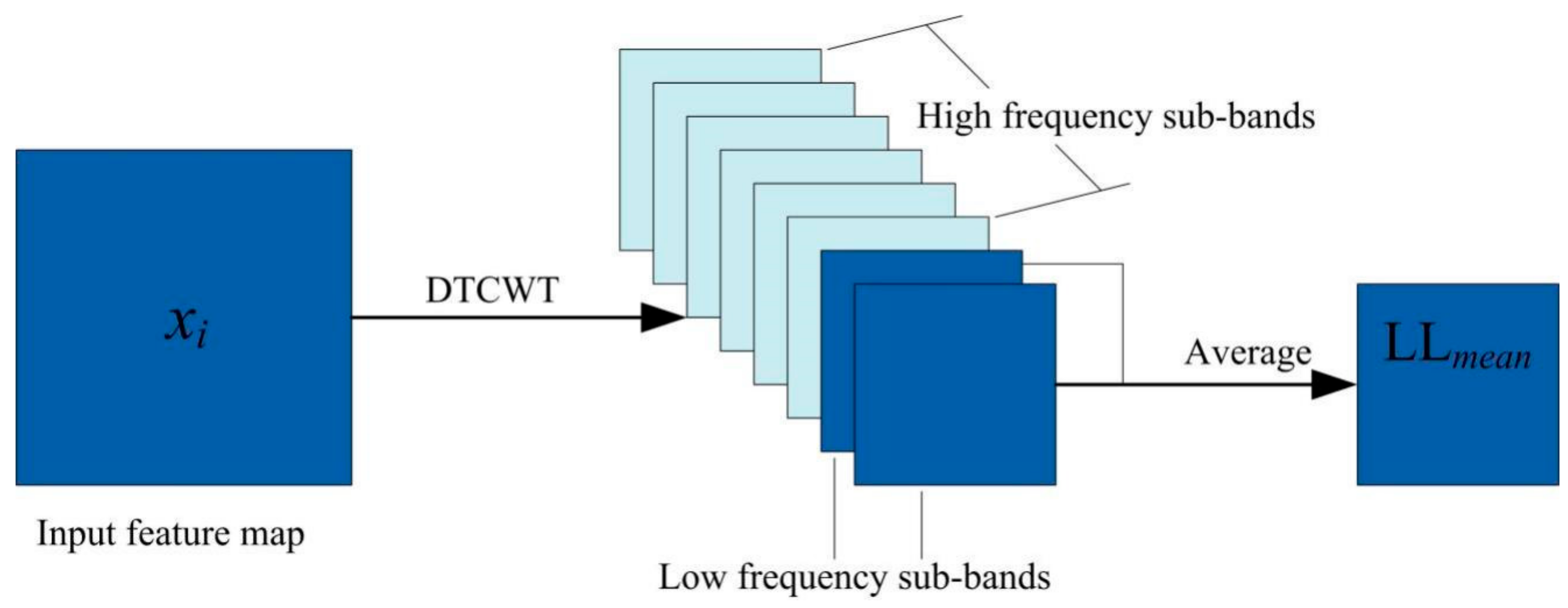
- A convolutional neural network based on dual-tree complex wavelet transform is constructed that aims to enhance the accuracy of change detection.
2. Related Works
2.1. SAR Image Preprocessing
2.2. DI Generation
2.3. Application of Classification to Change Detection
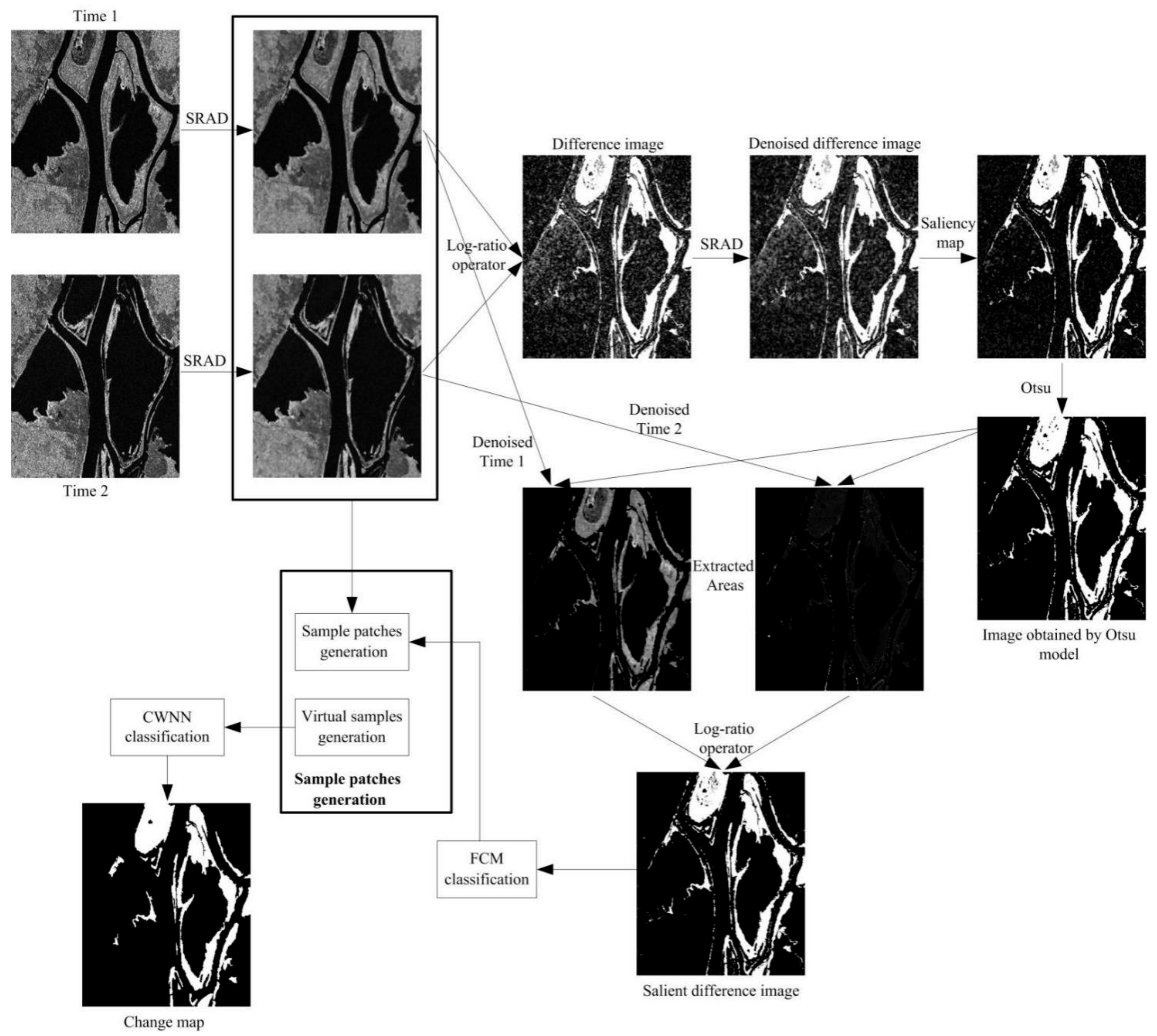
3. Proposed SAR Image Change Detection Method
3.1. Difference Image Generated by Log-Ratio Operator
3.2. Extraction of Salient Regions
3.3. Preclassification
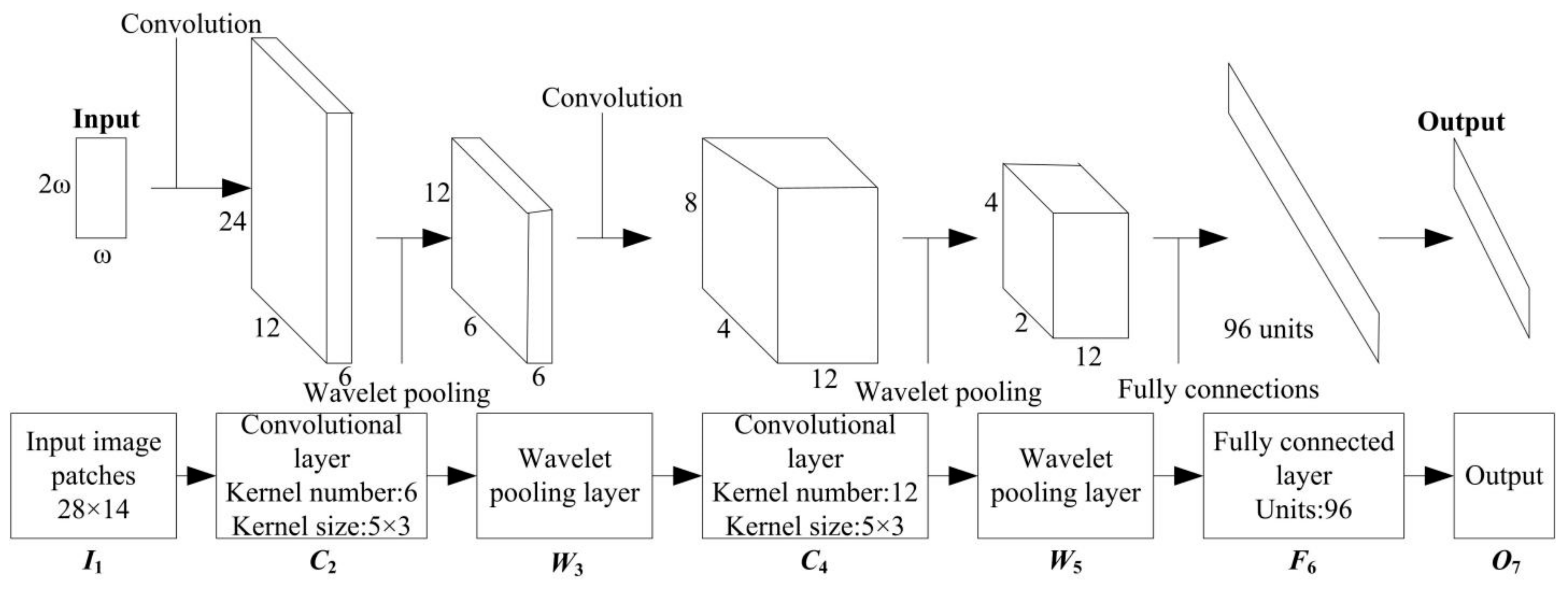
3.4. Classification by CWNN
4. Experimental Results and Discussions
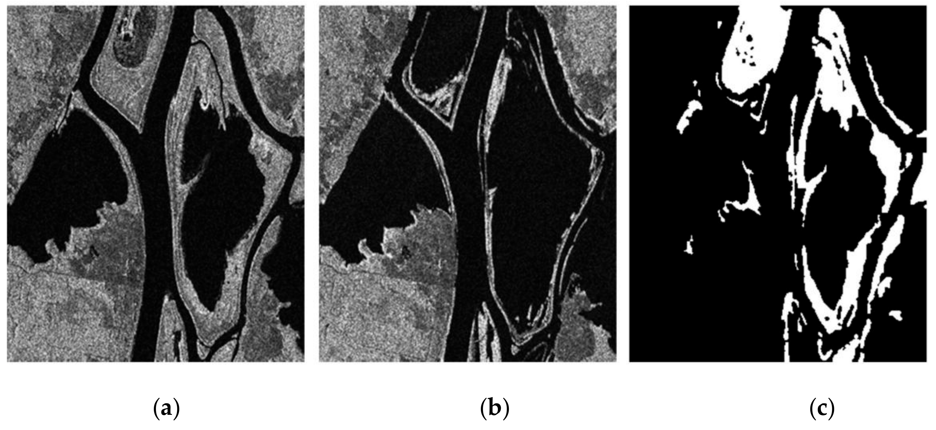
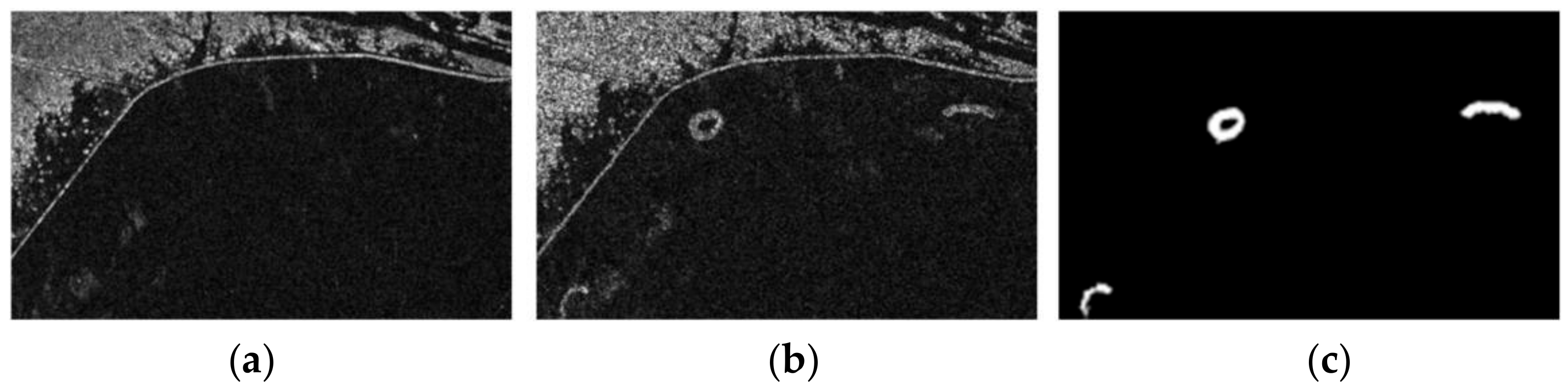
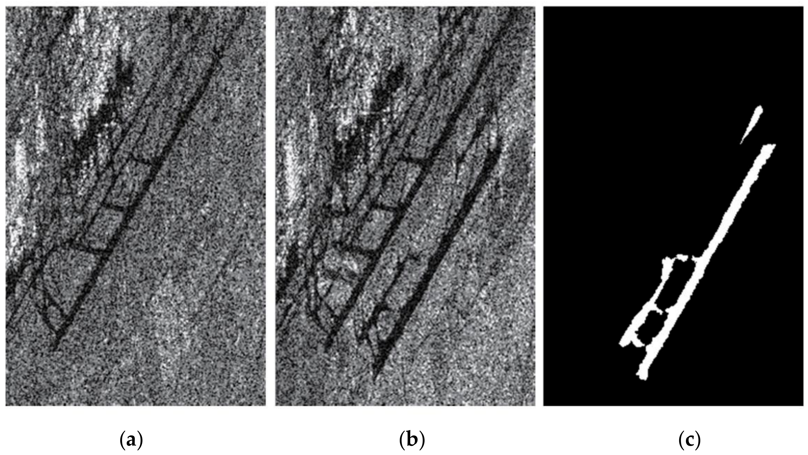
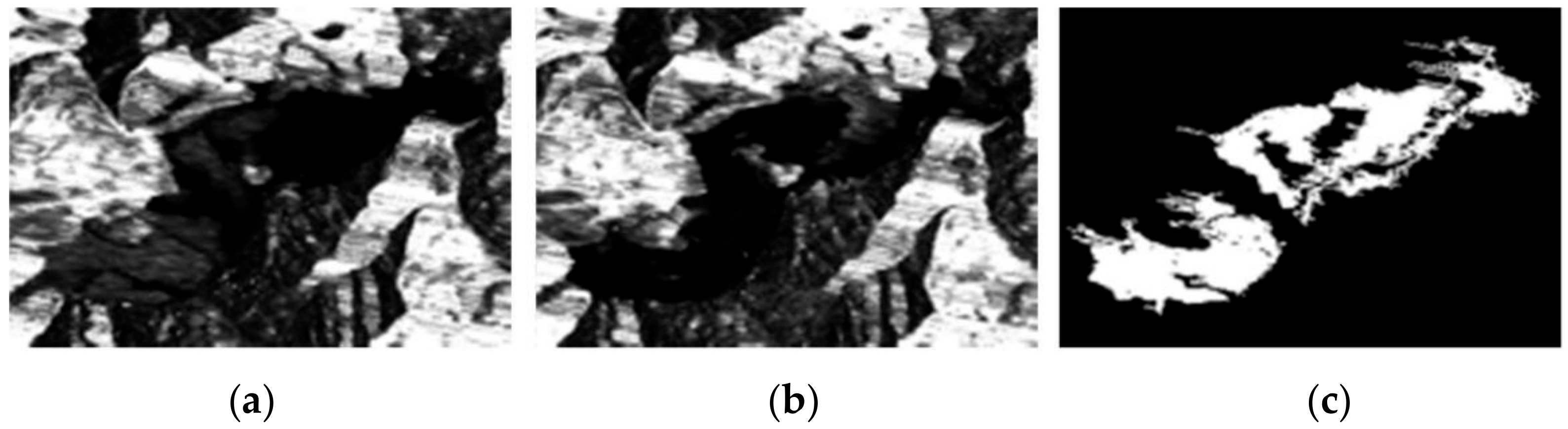
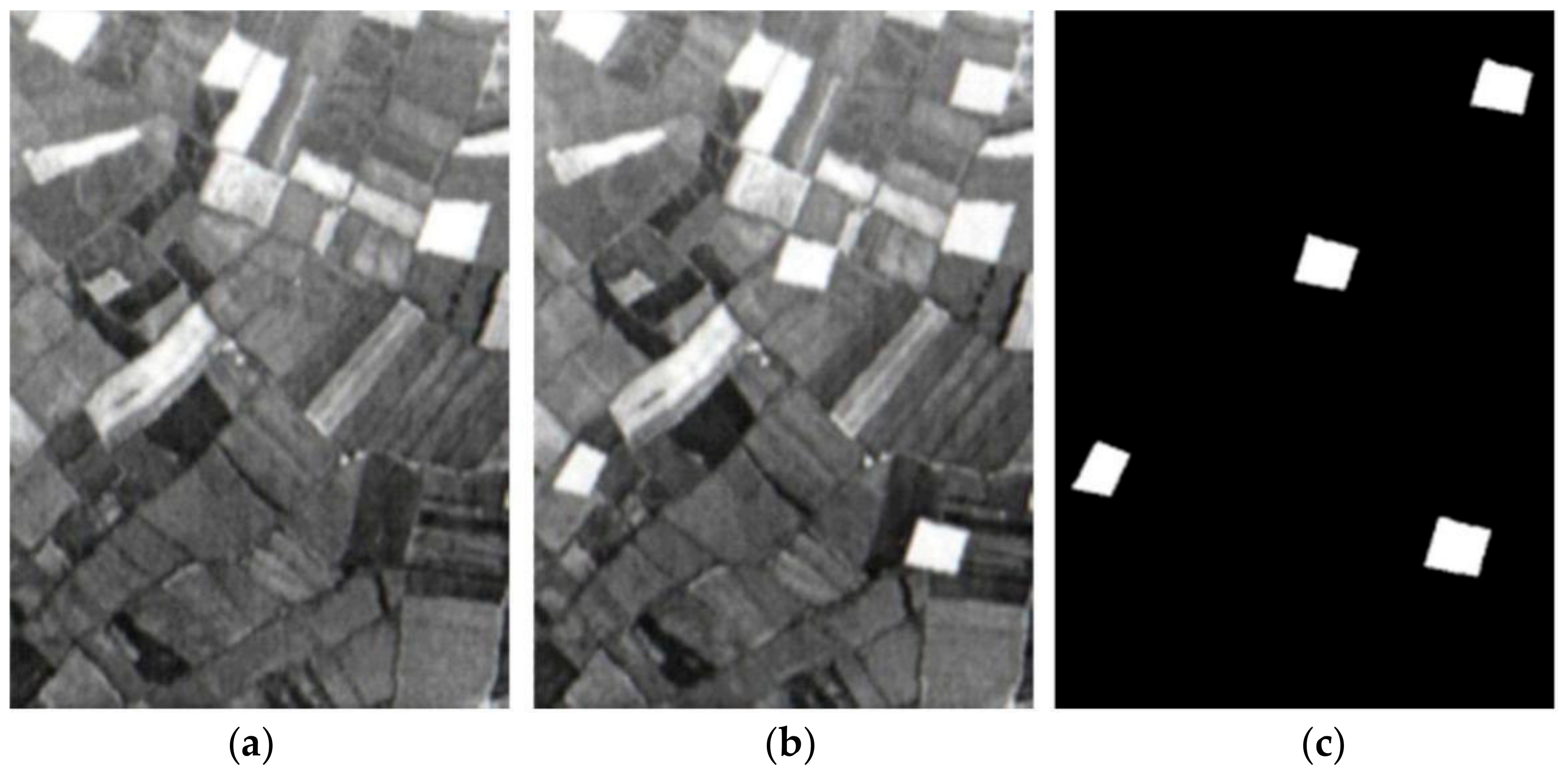
4.1. Data Set Descriptions
4.2. Experimental Settings
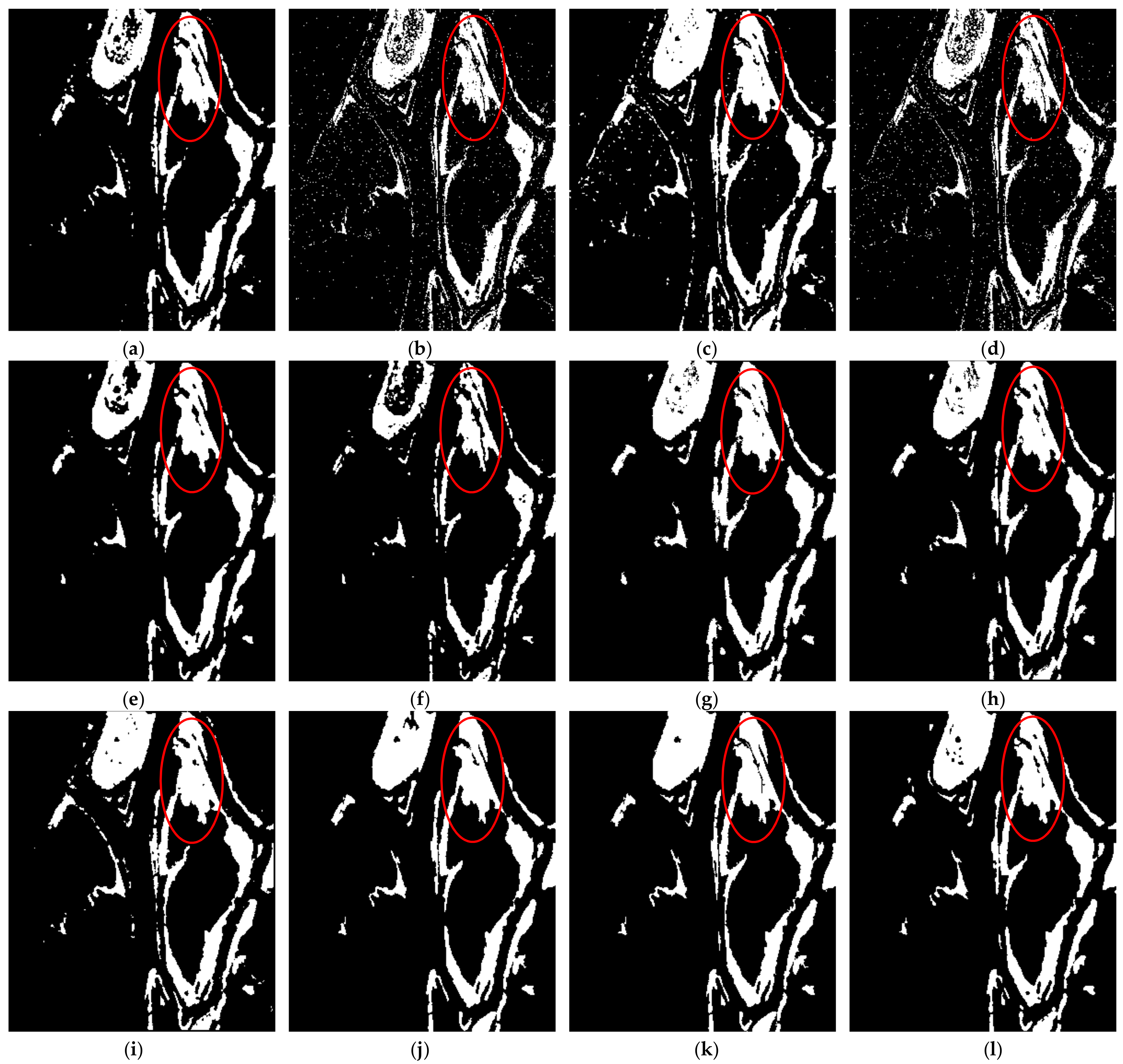
4.3. Results and Discussions
5. Conclusions
Author Contributions
Funding
Institutional Review Board Statement
Informed Consent Statement
Data Availability Statement
Conflicts of Interest
References
- Chen, H.; Zhang, K.; Xiao, W. Building change detection in very high-resolution remote sensing image based on pseudo-orthorectification. Int. J. Remote Sens. 2021, 42, 2686–2705. [Google Scholar] [CrossRef]
- Wang, C.; Wang, X. Building change detection from multi-source remote sensing images based on multi-feature fusion and extreme learning machine. Int. J. Remote Sens. 2021, 42, 2246–2257. [Google Scholar] [CrossRef]
- Huo, J.-Y.; Mu, L. Fast change detection method for remote sensing image based on method of connected area labeling and spectral clustering algorithm. J. Appl. Remote Sens. 2021, 15, 016506. [Google Scholar] [CrossRef]
- Zhao, J.; Liu, S.; Wan, J.; Yasir, M.; Li, H. Change detection method of high resolution remote sensing image based on DS evidence theory feature fusion. IEEE Access 2021, 9, 4673–4687. [Google Scholar] [CrossRef]
- Dong, H.; Ma, W.; Jiao, L.; Liu, F.; Li, L. A multiscale self-attention deep clustering for change detection in SAR images. IEEE Trans. Geosci. Remote Sens. 2021, 1–16. [Google Scholar] [CrossRef]
- Jung, J.; Yun, S.H. Evaluation of coherent and incoherent landslide detection methods based on synthetic aperture radar for rapid response: A case study for the 2018 Hokkaido Landslides. Remote Sens. 2020, 12, 265. [Google Scholar] [CrossRef] [Green Version]
- Yang, G.; Li, H.; Wang, W. Unsupervised change detection based on a unified framework for weighted collaborative repre-sentation with RDDL and fuzzy clustering. IEEE Trans. Geosci. Remote Sens. 2019, 57, 8890–8903. [Google Scholar] [CrossRef]
- Deledalle, C.-A.; Denis, L.; Tupin, F. Iterative weighted maximum likelihood denoising with probabilistic patch-based weights. IEEE Trans. Image Process. 2009, 18, 2661–2672. [Google Scholar] [CrossRef] [Green Version]
- Yu, Y.; Acton, S.T. Speckle reducing anisotropic diffusion. IEEE Trans. Image Process. 2002, 11, 1260–1270. [Google Scholar]
- Farhadiani, R.; Homayouni, S.; Safari, A. Hybrid SAR speckle reduction using complex wavelet shrinkage and non-local PCA-based filtering. IEEE J. Sel. Top. Appl. Earth Obs. Remote Sens. 2019, 12, 1489–1496. [Google Scholar] [CrossRef]
- Devapal, D.; Kumar, S.S.; Jojy, C. A novel approach of despeckling SAR images using nonlocal means filtering. J. Indian Soc. Remote Sens. 2016, 45, 443–450. [Google Scholar] [CrossRef]
- Hu, T.; Li, W.; Liu, N.; Tao, R.; Zhang, F.; Scheunders, P. Hyperspectral Image restoration using adaptive anisotropy total variation and nuclear norms. IEEE Trans. Geosci. Remote Sens. 2021, 59, 1516–1533. [Google Scholar] [CrossRef]
- Parrilli, S.; Poderico, M.; Angelino, C.V.; Verdoliva, L. A nonlocal SAR image denoising algorithm based on LLMMSE wavelet shrinkage. IEEE Trans. Geosci. Remote Sens. 2012, 50, 606–616. [Google Scholar] [CrossRef]
- Zhou, Y.; Shi, J.; Yang, X.; Wang, C.; Kumar, D.; Wei, S.; Zhang, X. Deep multi-scale recurrent network for synthetic aperture radar images despeckling. Remote Sens. 2019, 11, 2462. [Google Scholar] [CrossRef] [Green Version]
- Argenti, F.; Lapini, A.; Bianchi, T.; Alparone, L. A tutorial on speckle reduction in synthetic aperture radar images. IEEE Geosci. Remote Sens. Mag. 2013, 1, 6–35. [Google Scholar] [CrossRef] [Green Version]
- Zheng, Y.; Zhang, X.; Hou, B.; Liu, G. Using combined difference image and k-means clustering for sar image change detection. IEEE Geosci. Remote Sens. Lett. 2014, 11, 691–695. [Google Scholar] [CrossRef]
- Su, L.; Gong, M.; Sun, B. Change detection in synthetic aperture radar images based on non-local means with ratio similarity measurement. Int. J. Remote Sens. 2014, 35, 7673–7690. [Google Scholar] [CrossRef]
- Lou, X.; Jia, Z.; Yang, J.; Kasabov, N. Change detection in SAR images based on the ROF model semi-implicit denoising method. Sensors 2019, 19, 1179. [Google Scholar] [CrossRef] [Green Version]
- Wang, X.; Jia, Z.; Yang, J. Change detection in SAR images based on the logarithmic transformation and total variation de-noising method. Remote Sens. Lett. 2017, 8, 214–223. [Google Scholar] [CrossRef]
- Liu, L.; Jia, Z.; Yang, J. SAR image change detection based on mathematical morphology and the k-means clustering algorithm. IEEE Access 2019, 7, 43970–43978. [Google Scholar] [CrossRef]
- Zhang, Y.; Wang, C.; Ji, Y.; Chen, J.; Deng, Y.; Chen, J.; Jie, Y. Combining segmentation network and nonsubsampled contourlet transform for automatic marine raft aquaculture area extraction from sentinel-1 images. Remote Sens. 2020, 12, 4182. [Google Scholar] [CrossRef]
- Li, L.; Ma, H.; Jia, Z.; Si, Y. A novel multiscale transform decomposition based multi-focus image fusion framework. Multimed. Tools Appl. 2021, 80, 12389–12409. [Google Scholar] [CrossRef]
- Li, L.; Ma, H. Pulse coupled neural network-based multimodal medical image fusion via guided filtering and WSEML in NSCT domain. Entropy 2021, 23, 591. [Google Scholar] [CrossRef]
- Kollem, S.; Reddy, K.; Rao, D. Improved partial differential equation-based total variation approach to non-subsampled con-tourlet transform for medical image denoising. Multimed. Tools Appl. 2021, 80, 2663–2689. [Google Scholar] [CrossRef]
- Li, L.; Si, Y.; Wang, L. A novel approach for multi-focus image fusion based on SF-PAPCNN and ISML in NSST domain. Multimed. Tools Appl. 2020, 79, 24303–24328. [Google Scholar] [CrossRef]
- Li, L.; Ma, H. Saliency-Guided nonsubsampled shearlet transform for multisource remote sensing image fusion. Sensors 2021, 21, 1756. [Google Scholar] [CrossRef] [PubMed]
- Liu, Y.; Li, S.; Zhang, H. Multibaseline interferometric phase denoising based on kurtosis in the NSST domain. Sensors 2020, 20, 551. [Google Scholar] [CrossRef] [PubMed] [Green Version]
- Chen, P.; Zhang, Y.; Jia, Z.; Yang, J.; Kasabov, N. Remote sensing image change detection based on nsct-hmt model and its application. Sensors 2017, 17, 1295. [Google Scholar] [CrossRef] [Green Version]
- Li, S.; Fang, L.; Yin, H. Multitemporal image change detection using a detail-enhancing approach with nonsubsampled con-tourlet transform. IEEE Geosci. Remote. Sens. Lett. 2012, 9, 836–840. [Google Scholar]
- Zhou, W.; Jia, Z.; Yu, Y. SAR image change detection based on equal weight image fusion and adaptive threshold in the NSST domain. Eur. J. Remote. Sens. 2018, 51, 785–794. [Google Scholar]
- Shen, F.; Wang, Y.; Liu, C. Synthetic aperture radar image change detection based on Kalman filter and nonlocal means filter in the nonsubsampled shearlet transform domain. J. Appl. Remote Sens. 2020, 14, 016517. [Google Scholar] [CrossRef]
- Hou, B.; Wei, Q.; Zheng, Y. Unsupervised change detection in SAR image based on Gauss-log ratio image fusion and com-pressed projection. IEEE J. Sel. Top. Appl. Earth Obs. Remote Sens. 2014, 7, 3297–3317. [Google Scholar] [CrossRef]
- Zhang, Y.; Wang, S.; Wang, C.; Li, J.; Zhang, H. SAR image change detection using saliency extraction and shearlet transform. IEEE J. Sel. Top. Appl. Earth Obs. Remote Sens. 2018, 11, 4701–4710. [Google Scholar] [CrossRef]
- Gong, M.; Zhou, Z.; Ma, J. Change detection in synthetic aperture radar images based on image fusion and fuzzy clustering. IEEE Trans. Image Process. 2011, 21, 2141–2151. [Google Scholar] [CrossRef] [PubMed]
- Ma, J.; Gong, M.; Zhou, Z. Wavelet fusion on ratio images for change detection in SAR images. IEEE Geosci. Remote Sens. Lett. 2012, 9, 1122–1126. [Google Scholar] [CrossRef]
- Geng, J.; Ma, X.; Zhou, X.; Wang, H. Saliency-Guided deep neural networks for SAR image change detection. IEEE Trans. Geosci. Remote Sens. 2019, 57, 7365–7377. [Google Scholar] [CrossRef]
- Zheng, Y.; Jiao, L.; Liu, H.; Zhang, X.; Hou, B.; Wang, S. Unsupervised saliency-guided SAR image change detection. Pattern Recognit. 2017, 61, 309–326. [Google Scholar] [CrossRef]
- Wang, X.; Gao, F.; Dong, J. Change detection for synthetic aperture radar images based on pattern and intensity distinctiveness analysis. In Ninth International Conference on Graphic and Image Processing; International Society for Optics and Photonics: Bellingham, WA, USA, 2018; Volume 10615, p. 1061548. [Google Scholar]
- Majidi, M.; Ahmadi, S.; Shah-Hosseini, R. A saliency-guided neighbourhood ratio model for automatic change detection of SAR images. Int. J. Remote Sens. 2020, 41, 9606–9627. [Google Scholar] [CrossRef]
- Li, M.; Li, M.; Zhang, P. SAR image change detection using PCANet guided by saliency detection. IEEE Geosci. Remote Sens. Lett. 2019, 16, 402–406. [Google Scholar] [CrossRef]
- Moser, G.; Serpico, S. Generalized minimum-error thresholding for unsupervised change detection from SAR amplitude im-agery. IEEE Trans. Geosci. Remote Sens. 2006, 44, 2972–2982. [Google Scholar] [CrossRef]
- Celik, T.; Ma, K.-K. Multitemporal image change detection using undecimated discrete wavelet transform and active contours. IEEE Trans. Geosci. Remote Sens. 2010, 49, 706–716. [Google Scholar] [CrossRef]
- Hao, M.; Shi, W.; Deng, K.; Feng, Q. Superpixel-based active contour model for unsupervised change detection from satellite images. Int. J. Remote Sens. 2016, 37, 4276–4295. [Google Scholar] [CrossRef]
- Jia, L.; Li, M.; Zhang, P.; Wu, Y.; Zhu, H. SAR Image change detection based on multiple kernel k-means clustering with local-neighborhood information. IEEE Geosci. Remote Sens. Lett. 2016, 13, 856–860. [Google Scholar] [CrossRef]
- Shang, R.; Wen, A.; Liu, Y.; Jiao, L.; Stolkin, R. Synthetic aperture radar image change detection based on improved bilateral filtering and fuzzy C mean. J. Appl. Remote Sens. 2016, 10, 046017. [Google Scholar] [CrossRef]
- Li, Z.; Jia, Z.; Liu, L.; Yang, J.; Kasabov, N. A method to improve the accuracy of SAR image change detection by using an image enhancement method. ISPRS J. Photogramm. Remote Sens. 2020, 163, 137–151. [Google Scholar] [CrossRef]
- Zhang, X.; Liu, G.; Zhang, C.; Atkinson, P.M.; Tan, X.; Jian, X.; Zhou, X.; Li, Y. Two-Phase object-based deep learning for multi-temporal SAR image change detection. Remote Sens. 2020, 12, 548. [Google Scholar] [CrossRef] [Green Version]
- Gao, Y.; Gao, F.; Dong, J.; Wang, S. Change detection from synthetic aperture radar images based on channel weighting-based deep cascade network. IEEE J. Sel. Top. Appl. Earth Obs. Remote Sens. 2019, 12, 4517–4529. [Google Scholar] [CrossRef]
- Chan, T.-H.; Jia, K.; Gao, S.; Lu, J.; Zeng, Z.; Ma, Y. PCANet: A simple deep learning baseline for image classification? IEEE Trans. Image Process. 2015, 24, 5017–5032. [Google Scholar] [CrossRef] [PubMed] [Green Version]
- Gao, F.; Dong, J.; Li, B.; Xu, Q. Automatic change detection in synthetic aperture radar images based on PCANet. IEEE Geosci. Remote Sens. Lett. 2016, 13, 1792–1796. [Google Scholar] [CrossRef]
- Liu, T.; Li, Y.; Cao, Y.; Shen, Q. Change detection in multitemporal synthetic aperture radar images using dual-channel convolutional neural network. J. Appl. Remote Sens. 2017, 11, 1. [Google Scholar] [CrossRef] [Green Version]
- Duan, Y.; Liu, F.; Jiao, L.; Zhao, P.; Zhang, L. SAR Image segmentation based on convolutional-wavelet neural network and markov random field. Pattern Recognit. 2017, 64, 255–267. [Google Scholar] [CrossRef]
- Gao, F.; Wang, X.; Gao, Y.; Dong, J.; Wang, S. Sea ice change detection in sar images based on convolutional-wavelet neural networks. IEEE Geosci. Remote Sens. Lett. 2019, 16, 1240–1244. [Google Scholar] [CrossRef]
- Ma, J.; Zhou, Z.; Wang, B. Infrared and visible image fusion based on visual saliency map and weighted least square optimi-zation. Infrared Phys. Technol. 2017, 82, 8–17. [Google Scholar] [CrossRef]
- Gao, F.; Dong, J.; Li, B. Change detection from synthetic aperture radar images based on neighborhood-based ratio and ex-treme learning machine. J. Appl. Remote. Sens. 2016, 10, 046019. [Google Scholar] [CrossRef]
- Goyal, A.; Meenpal, T. Patch-Based dual-tree complex wavelet transform for kinship recognition. IEEE Trans. Image Process. 2021, 30, 191–206. [Google Scholar] [CrossRef]
- Celik, T. Unsupervised change detection in satellite images using principal component analysis and k-means clustering. IEEE Geosci. Remote Sens. Lett. 2009, 6, 772–776. [Google Scholar] [CrossRef]
- Sharma, A.; Gulati, T. Change detection in remotely sensed images based on modified log ratio and fuzzy clustering. Blockchain Technol. Innov. Bus. Process. 2017, 84, 412–419. [Google Scholar] [CrossRef]
- Li, H.-C.; Celik, T.; Longbotham, N.; Emery, W.J. Gabor Feature based unsupervised change detection of multitemporal SAR images based on two-level clustering. IEEE Geosci. Remote Sens. Lett. 2015, 12, 2458–2462. [Google Scholar] [CrossRef]
- Sumaiya, M.N.; Kumari, R.S.S. Logarithmic mean-based thresholding for SAR image change detection. IEEE Geosci. Remote Sens. Lett. 2016, 13, 1726–1728. [Google Scholar] [CrossRef]
- Gao, Y.; Gao, F.; Dong, J.; Wang, S. Sea ice change detection in SAR images based on collaborative representation. In Proceedings of the IGARSS 2018-2018 IEEE International Geoscience and Remote Sensing Symposium, Valencia, Spain, 22–27 July 2018; pp. 7320–7323. [Google Scholar]
- He, Y.; Jia, Z.; Yang, J.; Kasabov, N. Multispectral image change detection based on single-band slow feature analysis. Remote Sens. 2021, 13, 2969. [Google Scholar] [CrossRef]
- Yang, L.; Chen, Y.; Song, S.; Li, F.; Huang, G. Deep Siamese networks based change detection with remote sensing images. Remote Sens. 2021, 13, 3394. [Google Scholar] [CrossRef]
- Shao, P.; Shi, W.; Liu, Z.; Dong, T. Unsupervised change detection using fuzzy topology-based majority voting. Remote Sens. 2021, 13, 3171. [Google Scholar] [CrossRef]
- Wu, T.; Luo, J.; Fang, J.; Ma, J.; Song, X. Unsupervised object-based change detection via a weibull mixture model-based binarization for high-resolution remote sensing images. IEEE Geosci. Remote Sens. Lett. 2018, 15, 63–67. [Google Scholar] [CrossRef]
- Wu, T.; Luo, J.; Zhou, Y.; Wang, C.; Xi, J.; Fang, J. Geo-object-based land cover map update for high-spatial-resolution remote sensing images via change detection and label transfer. Remote Sens. 2020, 12, 174. [Google Scholar] [CrossRef] [Green Version]


| Place | Event | Pre-Data | Post-Data | Size | Satellite | Sensor Type |
|---|---|---|---|---|---|---|
| Ottawa | Flood | May 1997 | August 1997 | 290 × 350 | Radarsat-1 | SAR |
| Coastline | Flood | June 2008 | June 2009 | 450 × 280 | Radarsat-2 | SAR |
| De Gaulle Airport | Airstrip | July 1997 | October 1998 | 240 × 370 | ERS-1 | SAR |
| Wenchuan | Earthquake | 3 March 2008 | 16 June 2008 | 442 × 301 | ESA/ASAR | SAR |
| Village of Feltwell | Land cover variations | None | None | 335 × 470 | Daedalus 1268 ATM | SAR |
| Name/Reference | Parameter Settings |
|---|---|
| PCAKM [57] | |
| LROtsu [34] | None |
| MROtsu [34] | None |
| LRFCM [58] | None |
| GaborTLC [59] | |
| LMT [60] | The size of median filter is |
| PCANet [50] | |
| NRELM [55] | |
| NRCR [61] | neighborhood size: 3 |
| CWNN [53] | patch size |
| Proposed | patch size |
| FP | FN | OE | PCC(%) | KC(%) | |
|---|---|---|---|---|---|
| PCAKM [57] | 582 | 1901 | 2483 | 97.55 | 90.49 |
| LROtsu [34] | 2087 | 2741 | 4828 | 95.24 | 81.83 |
| MROtsu [34] | 2690 | 238 | 2928 | 97.12 | 89.80 |
| LRFCM [58] | 2106 | 2723 | 4829 | 95.24 | 81.85 |
| GaborTLC [59] | 253 | 2531 | 2784 | 97.26 | 89.07 |
| LMT [60] | 23 | 5266 | 5289 | 94.79 | 77.43 |
| PCANet [50] | 1087 | 985 | 2072 | 97.96 | 92.35 |
| NRELM [55] | 538 | 1242 | 1780 | 98.25 | 93.29 |
| NRCR [61] | 1723 | 777 | 2500 | 97.54 | 90.96 |
| CWNN [53] | 965 | 871 | 1836 | 98.19 | 93.22 |
| Proposed | 994 | 557 | 1551 | 98.47 | 94.32 |
| FP | FN | OE | PCC(%) | KC(%) | |
|---|---|---|---|---|---|
| PCAKM [57] | 39,426 | 25 | 39,451 | 68.69 | 4.30 |
| LROtsu [34] | 30,059 | 280 | 30,339 | 75.92 | 4.62 |
| MROtsu [34] | 43,863 | 39 | 43,902 | 65.16 | 3.63 |
| LRFCM [58] | 32,488 | 254 | 32,742 | 74.01 | 4.30 |
| GaborTLC [59] | 36,359 | 6 | 36,365 | 71.14 | 4.91 |
| LMT [60] | 139 | 650 | 789 | 99.37 | 63.59 |
| PCANet [50] | 14,387 | 8 | 14,395 | 88.58 | 14.00 |
| NRELM [55] | 6271 | 23 | 6294 | 95.00 | 28.33 |
| NRCR [61] | 21,633 | 12 | 21,645 | 82.82 | 9.15 |
| CWNN [53] | 13,754 | 51 | 13,805 | 89.04 | 14.13 |
| Proposed | 348 | 127 | 475 | 99.62 | 83.53 |
| FP | FN | OE | PCC(%) | KC(%) | |
|---|---|---|---|---|---|
| PCAKM [57] | 20,199 | 581 | 20,780 | 76.60 | 15.27 |
| LROtsu [34] | 11,446 | 1856 | 13,302 | 85.02 | 12.75 |
| MROtsu [34] | 29,189 | 441 | 29,630 | 66.63 | 10.15 |
| LRFCM [58] | 14,529 | 1644 | 16,173 | 81.79 | 11.60 |
| GaborTLC [59] | 17,051 | 436 | 17,487 | 80.31 | 19.59 |
| LMT [60] | 45 | 3248 | 3293 | 96.29 | 3.29 |
| PCANet [50] | 13,378 | 387 | 13,765 | 84.50 | 25.16 |
| NRELM [55] | 8060 | 761 | 8821 | 90.07 | 32.79 |
| NRCR [61] | 15,584 | 480 | 16,064 | 81.91 | 21.05 |
| CWNN [53] | 9794 | 541 | 10,335 | 88.36 | 30.79 |
| Proposed | 1156 | 1127 | 2283 | 97.43 | 64.31 |
| FP | FN | OE | PCC(%) | KC(%) | |
|---|---|---|---|---|---|
| PCAKM [57] | 939 | 7111 | 8050 | 93.95 | 76.27 |
| LROtsu [34] | 2574 | 6609 | 9183 | 93.10 | 74.00 |
| MROtsu [34] | 11,087 | 1723 | 12,810 | 90.37 | 70.95 |
| LRFCM [58] | 2527 | 6640 | 9167 | 93.11 | 74.01 |
| GaborTLC [59] | 689 | 8153 | 8842 | 93.35 | 73.27 |
| LMT [60] | 635 | 9333 | 9968 | 92.51 | 69.11 |
| PCANet [50] | 1366 | 5438 | 6804 | 94.89 | 80.73 |
| NRELM [55] | 988 | 6248 | 7236 | 94.56 | 79.04 |
| NRCR [61] | 582 | 8157 | 8739 | 93.43 | 73.52 |
| CWNN [53] | 578 | 9720 | 10,298 | 92.26 | 67.80 |
| Proposed | 2239 | 3159 | 5398 | 95.94 | 85.55 |
| FP | FN | OE | PCC(%) | KC(%) | |
|---|---|---|---|---|---|
| PCAKM [57] | 340 | 299 | 639 | 99.59 | 92.29 |
| LROtsu [34] | 857 | 244 | 1101 | 99.30 | 87.52 |
| MROtsu [34] | 4511 | 49 | 4560 | 97.10 | 63.42 |
| LRFCM [58] | 1327 | 184 | 1511 | 99.04 | 83.80 |
| GaborTLC [59] | 177 | 358 | 535 | 99.66 | 93.37 |
| LMT [60] | 1863 | 127 | 1990 | 98.74 | 79.87 |
| PCANet [50] | 27 | 1638 | 1665 | 98.94 | 75.22 |
| NRELM [55] | 25 | 2626 | 2651 | 98.32 | 54.16 |
| NRCR [61] | 10 | 1599 | 1609 | 98.98 | 76.13 |
| CWNN [53] | 45 | 2267 | 2312 | 98.53 | 62.36 |
| Proposed | 104 | 257 | 361 | 99.77 | 95.54 |
| FP | FN | OE | PCC(%) | KC(%) | |
|---|---|---|---|---|---|
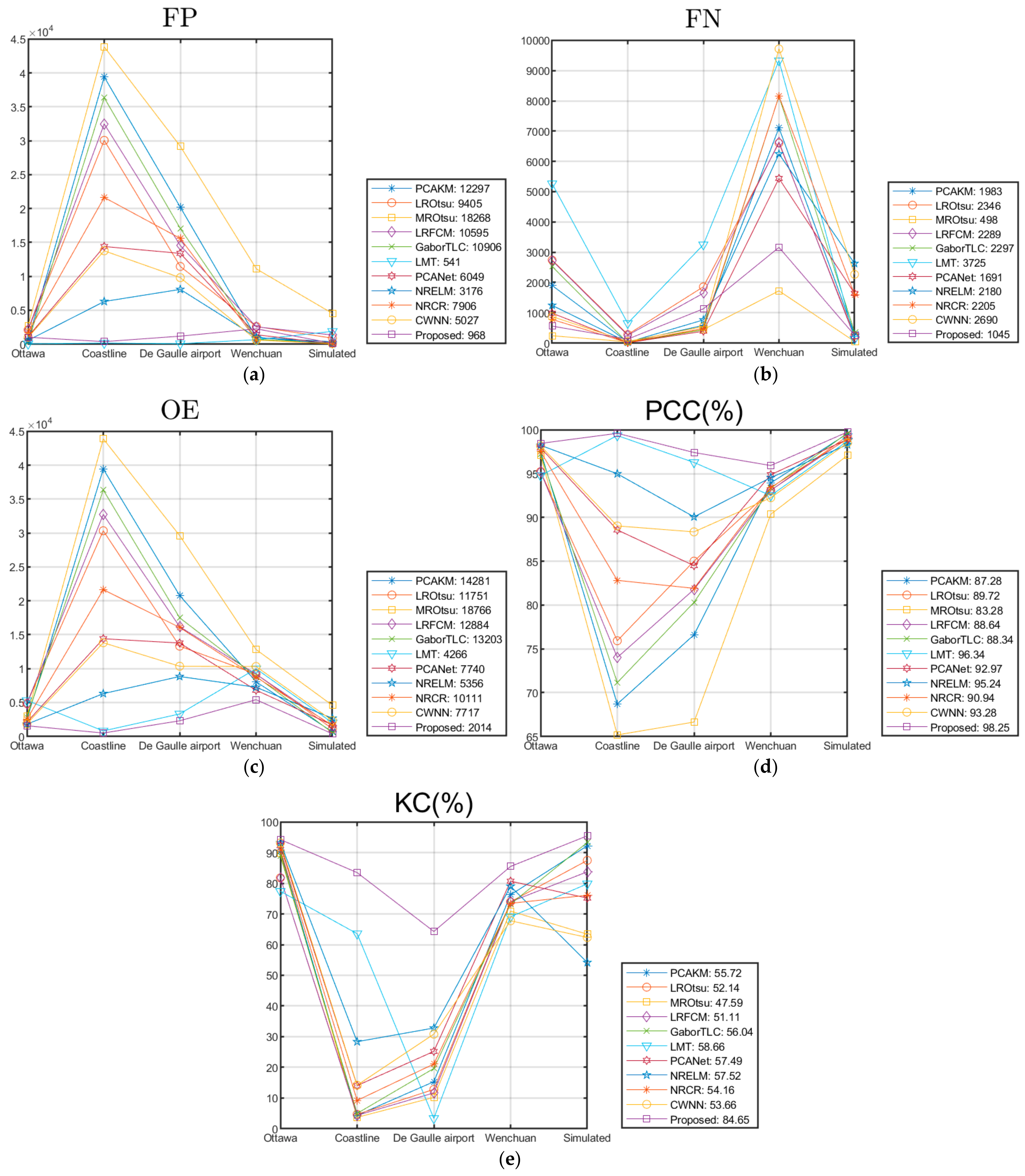
| PCAKM [57] | 12,297 | 1983 | 14,281 | 87.28 | 55.72 |
| LROtsu [34] | 9405 | 2346 | 11,751 | 89.72 | 52.14 |
| MROtsu [34] | 18,268 | 498 | 18,766 | 83.28 | 47.59 |
| LRFCM [58] | 10,595 | 2289 | 12,884 | 88.64 | 51.11 |
| GaborTLC [59] | 10,906 | 2297 | 13,203 | 88.34 | 56.04 |
| LMT [60] | 541 | 3725 | 4266 | 96.34 | 58.66 |
| PCANet [50] | 6049 | 1691 | 7740 | 92.97 | 57.49 |
| NRELM [55] | 3176 | 2180 | 5356 | 95.24 | 57.52 |
| NRCR [61] | 7906 | 2205 | 10,111 | 90.94 | 54.16 |
| CWNN [53] | 5027 | 2690 | 7717 | 93.28 | 53.66 |
| Proposed | 968 | 1045 | 2014 | 98.25 | 84.65 |
Publisher’s Note: MDPI stays neutral with regard to jurisdictional claims in published maps and institutional affiliations. |
© 2021 by the authors. Licensee MDPI, Basel, Switzerland. This article is an open access article distributed under the terms and conditions of the Creative Commons Attribution (CC BY) license (https://creativecommons.org/licenses/by/4.0/).
Share and Cite
Li, L.; Ma, H.; Jia, Z. Change Detection from SAR Images Based on Convolutional Neural Networks Guided by Saliency Enhancement. Remote Sens. 2021, 13, 3697. https://doi.org/10.3390/rs13183697
Li L, Ma H, Jia Z. Change Detection from SAR Images Based on Convolutional Neural Networks Guided by Saliency Enhancement. Remote Sensing. 2021; 13(18):3697. https://doi.org/10.3390/rs13183697
Chicago/Turabian StyleLi, Liangliang, Hongbing Ma, and Zhenhong Jia. 2021. "Change Detection from SAR Images Based on Convolutional Neural Networks Guided by Saliency Enhancement" Remote Sensing 13, no. 18: 3697. https://doi.org/10.3390/rs13183697
APA StyleLi, L., Ma, H., & Jia, Z. (2021). Change Detection from SAR Images Based on Convolutional Neural Networks Guided by Saliency Enhancement. Remote Sensing, 13(18), 3697. https://doi.org/10.3390/rs13183697