Abstract
Remote sensing image target detection is widely used for both civil and military purposes. However, two factors need to be considered for remote sensing image target detection: real-time and accuracy for detecting targets that occupy few pixels. Considering the two above issues, the main research objective of this paper is to improve the performance of the YOLO algorithm in remote sensing image target detection. The reason is that the YOLO models can guarantee both detection speed and accuracy. More specifically, the YOLOv3 model with an auxiliary network is further improved in this paper. Our model improvement consists of four main components. Firstly, an image blocking module is used to feed fixed size images to the YOLOv3 network; secondly, to speed up the training of YOLOv3, DIoU is used, which can speed up the convergence and increase the training speed; thirdly, the Convolutional Block Attention Module (CBAM) is used to connect the auxiliary network to the backbone network, making it easier for the network to notice specific features so that some key information is not easily lost during the training of the network; and finally, the adaptive feature fusion (ASFF) method is applied to our network model with the aim of improving the detection speed by reducing the inference overhead. The experiments on the DOTA dataset were conducted to validate the effectiveness of our model on the DOTA dataset. Our model can achieve satisfactory detection performance on remote sensing images, and our model performs significantly better than the unimproved YOLOv3 model with an auxiliary network. The experimental results show that the mAP of the optimised network model is 5.36% higher than that of the original YOLOv3 model with the auxiliary network, and the detection frame rate was also increased by 3.07 FPS.
1. Introduction
Target detection is a hot topic in the field of computer vision. The aim is to find the target object as well as the target location in a single image. With the development of target detection algorithms, remote sensing image (RSI) target detection has also evolved tremendously. Nowadays, remote sensing image target detection technology is widely used in practical applications, such as environmental supervision, disaster assessment, military investigations, and urban planning [1,2].
In recent years, benefits from the development of convolutional neural networks (CNNs), machine learning-based target detection algorithms have been further developed, resulting in extensive research in the field of computer vision, especially in target detection. CNN models exhibit powerful feature extraction capabilities and excellent performance that have led to their tremendous development in the field of target detection, and they are gradually being applied to RSI target detection.
As the most common deep learning model, CNN can already complete various image algorithm tasks very well, including semantic segmentation [3,4], image classification [5,6], object detection [7,8], and image super-resolution [9]. In the research of target detection, R-CNN [10] is the first deep learning algorithm, which is a CNN-based feature learning model. This model is a good substitute for traditional manual features and significantly improves the performance of the CNN model. The original CNN model classifier mostly uses the SVM module, but in the design of the R-CNN model in order to better adapt to the design of the neural network, the classifier uses softmax and the regression of the Bounding Box is added to the model. With the help of the sliding window idea, a pooling layer, called region of interest, was first applied to R-CNN. The purpose of the pooling layer is to convert the feature representation of each region of interest into a fixed length vector. Fast R-CNN [7] performs feature extraction on the original input image based on R-CNN, and maps all regional suggestions to the extracted feature map. In 2017, the advent of Faster R-CNN [11] further overcame the computational burden in the generation of Fast R-CNN region proposals. Subsequent developments on the basis of Faster R-CNNs, such as Mask R-CNN [12], which is a feature pyramid network (FPN) used as a backbone network to generate multi-scale feature maps with the addition of a mask prediction branch to detect the exact boundaries of each instance. The above method is generally divided into two stages: region proposal generation and object detection from region proposals. Therefore, these methods are often referred to as two-stage target detection methods. Two-stage target detection is too slow and the efficiency of detection becomes an issue. However, in 2015 the YOLO [13] algorithm was proposed to improve the problem of slow detection in target detection tasks. In the YOLO model, the input image is divided into grid cells, and each cell is responsible for detecting a fixed number of objects. YOLO is usually much faster than the two-stage object detector, but the detection performance is poor. After YOLO, YOLOv2 [14] and YOLOv3 [15] have been proposed one after the other, and improve performance by using a more powerful backbone network and perform object detection on multiple scales. More specifically, the YOLOv3 model uses FPN [16] as the backbone network, so it can perform more powerful feature extraction and detection on different scales.
Along with the development of target detection algorithms for usual objects, RSI target detection algorithms have also been extensively researched, which were applied in scene classification [17], object detection [18,19], and so forth. The existing RSI target detection algorithms can be roughly divided into four categories: (1) Method based on template matching; (2) Knowledge-based target detection method; (3) Object detection algorithm based on object analysis; and (4) Based on machine learning [1]. Among the above mentioned methods, the method based on machine learning has been favored by many scholars due to its strong robustness, has been extensively studied, and has obtained breakthrough development [20,21,22]. The RSI target detection method based on deep learning gets rid of the machine learning method that uses tedious manual features, can automatically learn features from deep networks, and is more robust. R-CNN is the first deep learning architecture used for RSI detection. Chen et al. [23] introduced a rotation-invariant method in R-CNN, which solves the problem of inaccurate detection due to arbitrary target orientation during remote sensing image detection. Zhang et al. [24] introduced a hierarchical feature coding network, which is often used for the learning of some robust expressions, and has been tested on high-resolution remote sensing images to prove the effectiveness of the method. Because R-CNN has achieved great success in RSI detection, subsequent research also began to apply the Faster R-CNN model to RSI detection. For example, because the use of horizontal anchors in RPN makes it more sensitive to rotating objects, Li et al. [25] solved this problem by using multi-angle anchors. The proposed method can effectively detect geospatial object of arbitrary orientations. Due to the slow speed of the two-stage detection and the great success of the one-stage image detection algorithm, domestic and foreign scholars have also begun to study various regression-based remote sensing image target detection algorithms. Refs. [8,26,27,28,29,30,31], for example, in order to realize real-time vehicle detection of remote sensing images, the SSD model is extended [30] to increase the detection speed. Since horizontal anchors cannot detect objects with directional angles, Ref. [31] uses directional anchors in the SDD [32] framework, so that the model can detect objects with directional angles. In order to further improve the performance of RSI target detection, some more advanced algorithms have been proposed, such as hard example mining [26], multi-feature fusion [33], transfer learning [34], non-maximum suppression [35] and other algorithms.
When performing target detection in RSI, an image had a shooting range of approximately 10–30 km. Under such a huge shooting range, some relatively small objects, such as cars, ships and airplanes, and so forth, occupied only a few pixels in the image, which led to a high rate of missed and false detections when detecting RSIs. To ensure accuracy while guaranteeing detection speed, YOLOv3 was used as the basic algorithm in this study. However, the RSI detection performance of YOLOv3 is not satisfactory. Considering the above reasons, RSI target detection became very challenging. Therefore, this study developed the detection of the remote sensing image based on the optimized YOLO v3 network. In this study, an auxiliary network for target object detection on RSI was introduced. The purpose of the model was to detect small targets in RSI scenes with relatively high accuracy. The method was constructed based on a recent study [36], which was developed for driving scenarios in optical images. RSIs have different scales, yet YOLOv3 requires a fixed size input. Therefore, an image preprocessing module was added to divide the input image into a fixed size. Considering the increase in the network structure resulting in a larger amount of calculation [36], in order to solve the problem, the Squeeze-and-Excitation (SE) attention mechanism used in [36] was replaced by a convolutional block attention module (CBAM) [37] to connect auxiliary networks. On the other hand, previously applied methods could lead to insufficient feature fusion and thus cause over-fitting. To speed up convergence of the loss function and strengthen the regression ability of the Bounding Box, the DIoU loss function is used in this paper. In order to enhance the robustness of the model, the adaptive feature fusion (ASFF) [38] method was introduced. Specifically, the original feature pyramid network (FPN) of YOLO v3 was replaced with adaptive feature fusion.
The main contributions of this study are summarized as follows:
- The auxiliary network is introduced in RSI target detection, and the original SE attention mechanism in the auxiliary network is replaced by CBAM in order to make some specific features in the target more easily learned by the network;
- An image blocking module is added to the network to ensure the size of the input images are a fixed size;
- Adaptive feature fusion is used in the rear and serves to filter conflicting information spatially to suppress inconsistencies arising from back propagation, thereby improving the scale invariance of features and reducing inference overhead;
- To increase the training speed of the network, the DIoU loss function is used in the calculation of the loss function. The role of DIoU is that it can directly minimize the distance between two target frames and accelerate the convergence of losses.
2. Materials and Methods
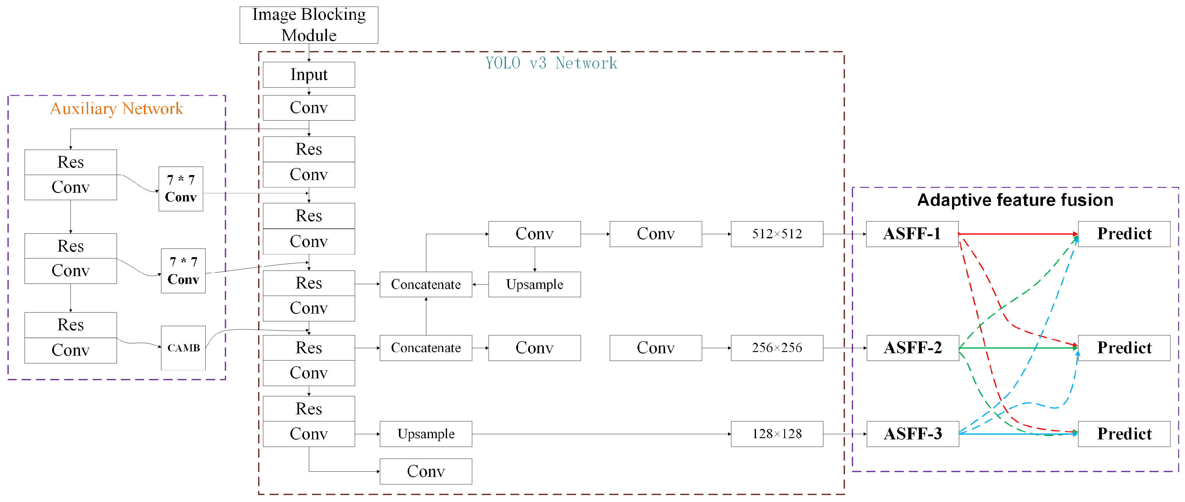
The target detection of remote sensing images needed to ensure the real-time and accuracy of detection. The detection speed of the two-stage baseline was relatively slow. YOLOv3 as a representative of one-stage target detection algorithms can satisfy both detection performance and speed requirements, was selected as the most basic model. Meanwhile, since most target information in remote sensing images occupied only a few pixels, considering some relatively small amount of image information being lost by the original YOLOv3 when extracting features, hence the purpose of this study was to improve the robustness of YOLOv3 in extracting small target information. The pipeline of the network structure is illustrated in Figure 1. The improvement of the network structure consists of three main components: Firstly, an image blocking module is added to the network input so that the RSIs fed into the network are a fixed size; secondly, replacing the SE attention mechanism in the auxiliary network [36] with CBAM [37] allows the network to better learn specific target features; and finally, adaptive feature fusion is used at the rear, which serves to filter conflicting information spatially to suppress inconsistency when gradient backpropagation is used, thus improving the scale invariance of the features and reducing the inference overhead.
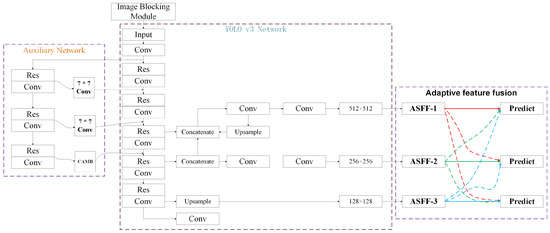
Figure 1.
The overall pipeline of the method used in this paper.
2.1. Image Blocking Module
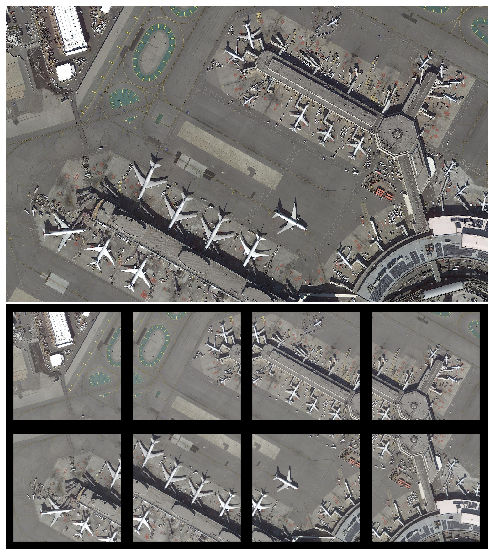
The remote sensing image target detection model improved in this paper aims to enhance the original model’s ability to detect small targets. Our network requires a fixed size input image, but remote sensing images of different sizes cannot be directly input into our network, so an image blocking module is added to the input side of the network, which serves to subdivide each input remote sensing image into sub images of the same size for the network to proceed to the next step. The effect of image blocking is shown in Figure 2. The top image is the original image, and the bottom image is divided into one fixed size sub-image.
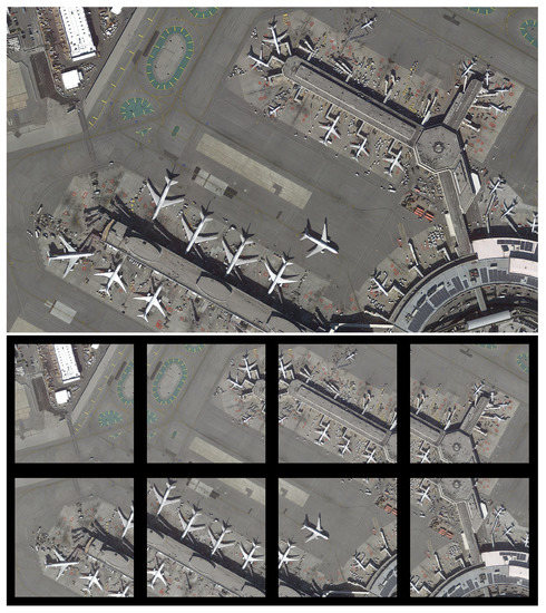
Figure 2.
Demonstrate the effect of processing the input image into a fixed size.
2.2. Convolutional Block Attention Module
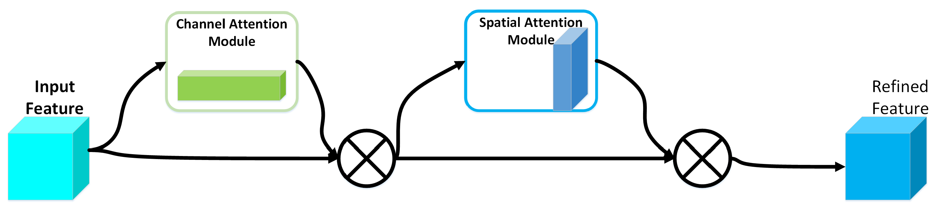
The network used in this study was in the form of an auxiliary network. Instead of using the channel attention Squeeze-and-Excitation module applied in the previous study [36], the Convolution Block Attention Module [37] was used to connect the backbone network and the auxiliary network. The structure of CBAM [37] is shown in Figure 3.

Figure 3.
The structure of CBAM.
The CBAM module sequentially infers the attention map along through two independent dimensions (channel and space). The attention map was then multiplied with the input feature map for adaptive feature optimization. It is illustrated in Figure 3 that the output result of the convolutional layer first passed through a channel attention module. After the weighted result was obtained, it passed through a spatial attention module, where finally the result was weighted.
The input feature maps are processed by global maximum pooling and global average pooling respectively, and then by a multi layer perceptron (MLP), respectively. The output of the MLP is based on an element summation operation. A sigmoid function activation operation is then performed to generate the final channel attention feature map. The channel attention feature map and the input special diagnostic map are element-wise multiplied to generate the input features required by the spatial attention module. The formula for channel attention is as follows:
where F represents the feature map of the input; and represents the features after global average pooling and global maximum pooling, respectively; and represent the two-layer parameters in the multilayer perceptron model. It is worth noting that the features between and in the multilayer perceptron model in this article need to be processed using ReLU as the activation function. In the spatial attention mechanism, average pooling and maximum pooling are still used to compress the input feature map. However, the compression here becomes the compression at the channel level, and the input features are averaged and maximized in the channel dimension, respectively. Finally, two two-dimensional features are obtained, which are spliced together according to the channel dimensions to obtain a feature map with a channel number of two, and then a hidden layer containing a single convolution kernel is used to perform convolution operations on them. The final feature is consistent with the input feature mapping in the spatial dimension. The feature maps after the maximum pooling and average pooling operations are and . The formula for spatial attention is as follows:
where represents an activation function. More than one convolution kernel was used within the convolution layer in this study.
2.3. Adaptive Feature Fusion
The feature pyramid method was used for feature fusion in YOLOv3. The significance of the feature pyramid is that each prediction branch effectively combines information from the deep network feature map with the location information from the shallow network feature map. However, there is rich spatial information in the shallow layer of the network and richer semantic information in the deep network. So the shallow layer is suitable for detecting small targets and the deep layer is suitable for detecting large targets. Therefore, the adaptive feature fusion (ASFF) [38] method used in this paper can be regarded as a filter, which can filter out the activation values of small objects in the deep layer and combine the feature values corresponding to large objects in the shallow feature map to enrich the information of large objects in the deep layer. It is important to emphasise here that, by performing convolution as well as pooling operations in the network, we can obtain feature mappings of different sizes from the convolution layer, and it is from these feature mappings generated in the convolution operation that we perform adaptive feature fusion. Different from the method of using element-by-element accumulation and cascading to integrate multi-level features, the key of adaptive feature fusion [38] is to autonomously learn the spatial weight of each scale fusion. Adaptive feature fusion is divided into two main parts: (1) the same scale transformation; (2) adaptive fusion.
2.3.1. Scale Transformation
The resolution level of the feature is represented by . For level l, adjust the feature size in other levels from to the same size as . Because the features in the three layers of YOLO v3 have different resolutions, that is, there are different numbers of channels, the up-sampling and down-sampling strategies are modified at each scale. For upsampling, a convolutional layer is first applied to compress the number of feature channels to l, and features with larger scales will be inserted separately. For downsampling, a ratio of 1/2 is used, and a convolutional layer of 3 to 3 with a step size of 2 is used to simultaneously modify the number of channels and resolution. For a sampling ratio of 1/4, a maximum pooling layer with a step size of 2 is added before the convolution operation with a step size of 2.
2.3.2. Adaptive Fusion
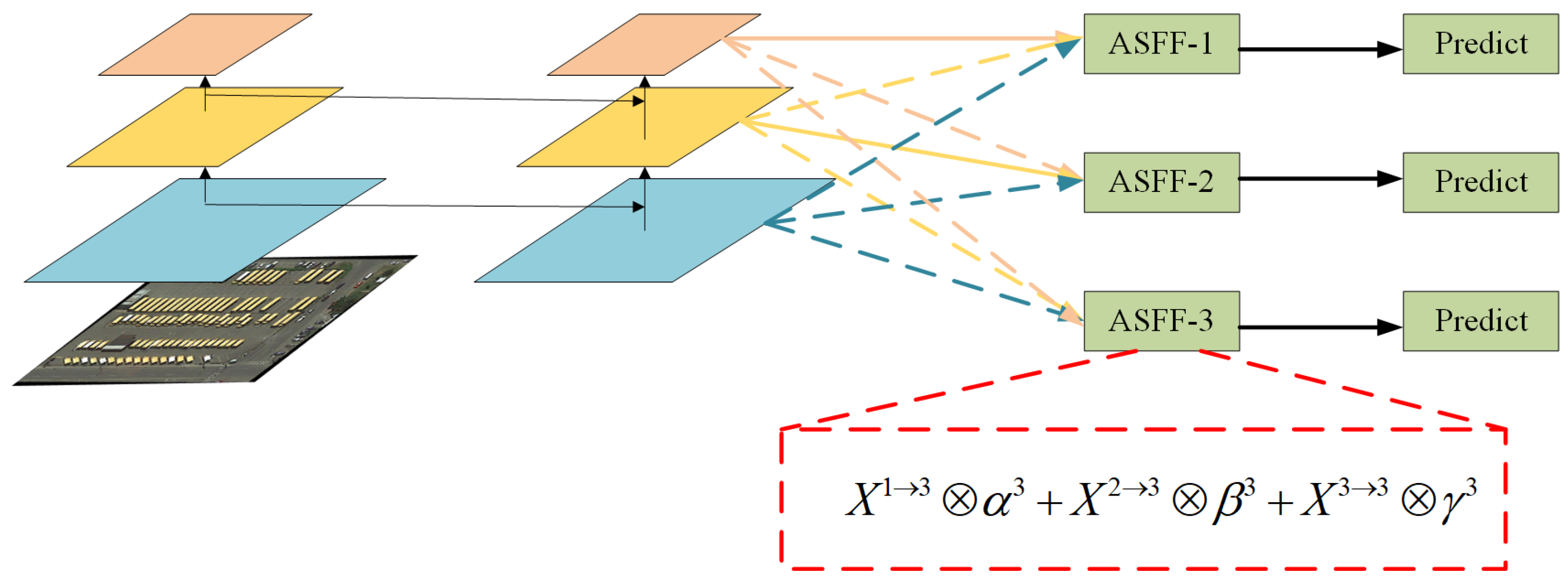
As shown in Figure 4, taking ASFF-3 as an example, the process of feature fusion is depicted in the red box, where , and are the features from level 1, level 2 and level 3 respectively, and the features from the different layers are multiplied by the weight parameters , , and are summed to obtain the new fused feature ASFF-3. It is expressed as the following formula:
where implies the vector of the feature maps y among channel, are the weights from three different feature levels to level l, which is learned by the network adaptively. It should be noted that are simple scalars and can be shared among all channels. Let and , and define:
where are defined by softmax function and respectively as control parameters. Using the convolutional layer of to calculate the weight , respectively, the scalar graph can be learned by standard back propagation. Using this method, features at all levels can be adaptively aggregated to each scale.
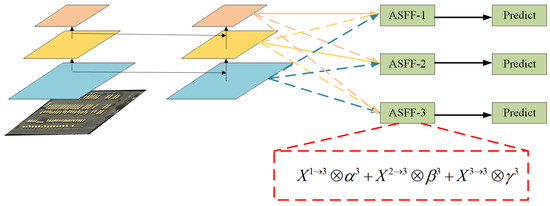
Figure 4.
Adaptive feature fusion.
2.4. Loss Function
There are overlapping and intersecting targets in remote sensing images. The loss function of the YOLOv3 model with an auxiliary network is GIoU [36]. This loss function converges relatively slowly, so this paper uses DIoU, which converges relatively quickly as the loss function. This section mainly introduces the following two functions of using DIoU Loss [39]:
- The normalized distance between predicted box and target box was directly minimized for achieving faster convergence;
- The regression was made more accurate and faster when having an overlap of inclusion with target box.
Generally, the Iou-Based loss can be defined as:
where is the penalty term for predicted box B and target box .
2.4.1. Distance-IoU Loss
In order to solve the problem of slow convergence in the original loss function, the normalized distance was minimized between the center points of the two bounding boxes in this study, and the penalty term can be defined as:
where and denote the central points of B and , is the Euclidean distance, and c is the diagonal length of the smallest enclosing box covering the two boxes. Then, the DIoU loss function can be defined as:
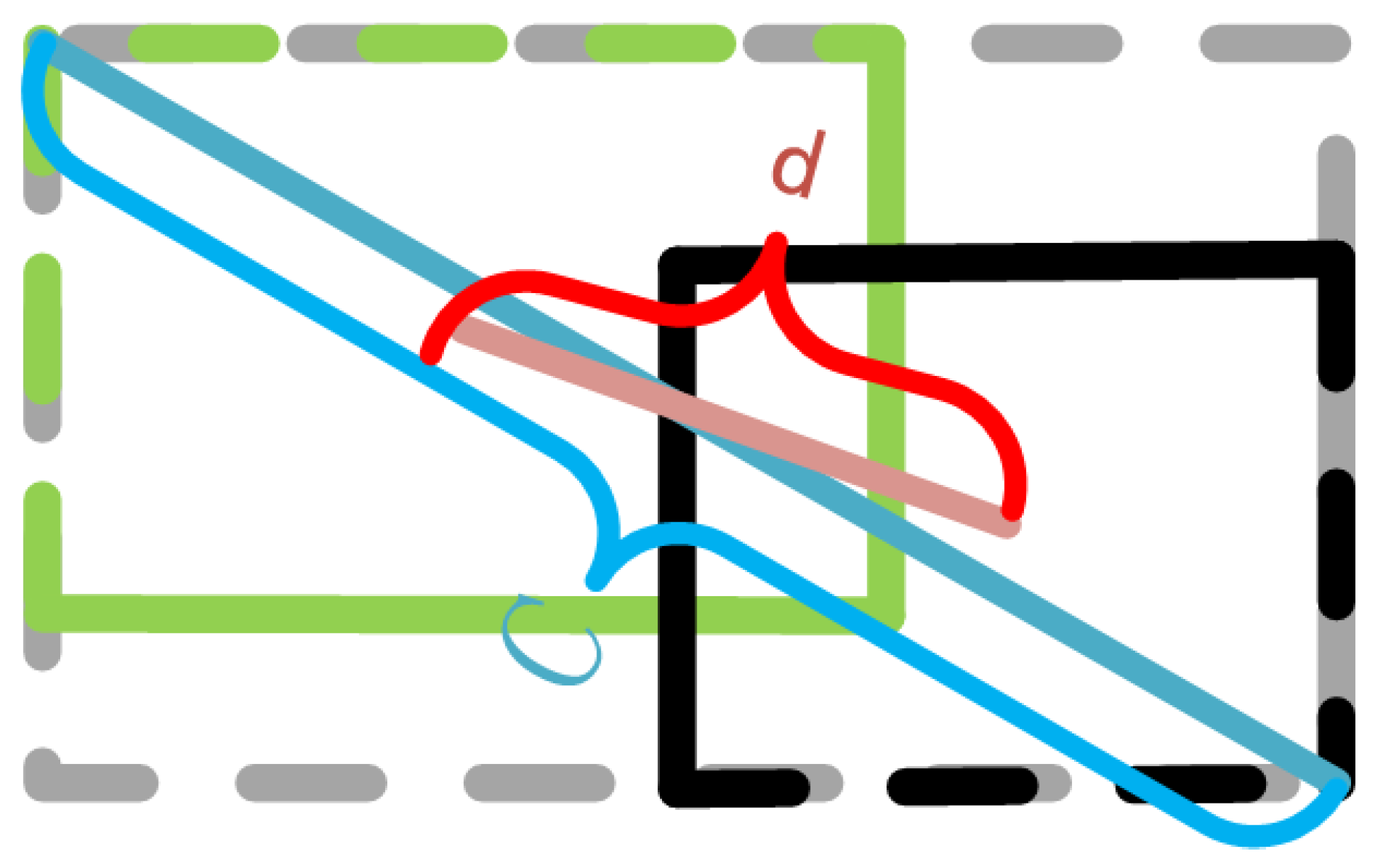
As shown in Figure 5, the penalty term of DIoU loss directly minimizes the distance between two central points, while GIoU loss aims to reduce the area of .

Figure 5.
DIoU loss for bounding box regression, where the normalized distance between central points can be directly minimized. c is the diagonal length of the smallest enclosing box covering two boxes, and is the distance of central points of two boxes.
2.4.2. Non-Maximum Suppression Using DIoU
In original Non-Maximun Suppression (NMS), the IoU metric is used to suppress the redundant detection boxes, where the overlap area is the unique factor, often yielding false suppression for the cases with occlusion. However, the DIoU loss is a better criterion for NMS, because not only the overlap area but also the central point distance between two boxes should be considered in the suppression criterion. For the predicted box M with the highest score, the DIoU-NMS can be formally defined as:
where box is removed by simultaneously considering the IoU and the distance between central points of two boxes, is the classification score and is the threshold. In the research, it is found that two boxes with center points far apart may correspond to different targets, so this kind of box should not be removed. The process of is as follows: 1. Set the confidence threshold of the target box, in this paper the threshold is set to 0.7; 2. Arrange the list of candidate boxes in descending order according to the confidence, select the box with the highest confidence A to add to the output list and remove it from the list of candidate boxes; 3. Calculate the DIoU value of A and all the boxes in the list of candidate boxes, delete the candidate boxes larger than the threshold and repeat the above process; 4. List is empty, return to the output list; 5. When the DIoU value of the highest scoring prediction box M is compared to the DIoU value of the other , the score of remains, otherwise, when the DIoU is greater than the threshold value, the value is set to 0, it is filtered out.
3. Experimental Results and Discussion
In this section, we have trained and tested our model on the DOTA dataset and our model is deployed in the Tensorflow 2.0 framework. All experiments were implemented on the workstation with an Intel (R) Xeon(R) CPU E5-2640 v4 @ 2.40GHz, two NVIDIA GeForce RTX 2080 Ti and 32 GB of memory.
3.1. DOTA Datasets and Evaluation Indicators
The DOTA dataset used in this experiment was DOTA 1.0, which contained 2806 RSI, as well as 188,282 instances in 15 categories. The labeling method was a quadrilateral of any shape and direction determined by four points (which was different from the traditional parallel bounding box with opposite sides). A total of 15 image categories were obtained, including 14 main categories. The category image of the DOTA dataset was shown in Figure 6. The dataset was divided into 1/6 verification set, 1/3 test set, and 1/2 training set. There are 1403 images used for training and 935 images used for testing in this paper.
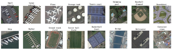
Figure 6.
DOTA Dataset Category Display.
The label data format in the DOTA dataset was inconsistent with the label data format required by the YOLO model. Therefore, the DOTA label data format was converted into the YOLO label data format in batches.
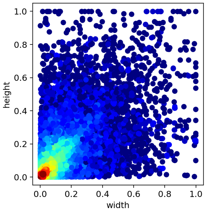
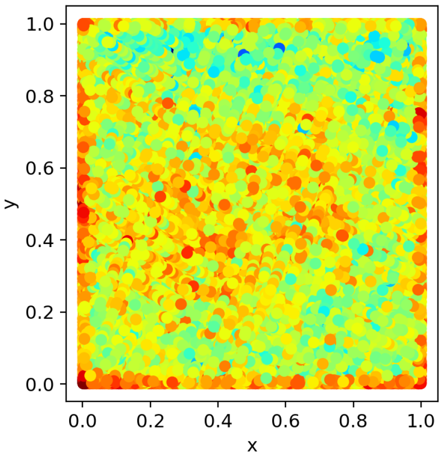
In order to visualise the varying sizes of targets and the random distribution of targets in the DOTA dataset, a heat map is used to represent the situation. The heat map of the target dimensions is shown in Figure 7. The dimensions of the target are normalised. The horizontal coordinates represent the width of the target and the vertical coordinates represent the length of the target. From the heat map in Figure 7, it can be seen that the targets in the DOTA dataset are of different sizes, which can prove that the method in this paper is effective for targets of different sizes. According to the target position heat map shown in Figure 8, it could be seen that the targets to be detected are distributed in various locations. The position of the target in the image is normalised and the horizontal and vertical coordinates represent the normalised position of each target in the image.

Figure 7.
Target Size Heat Map.
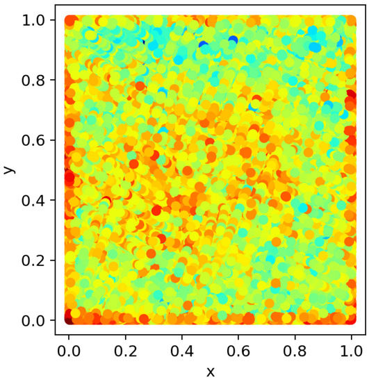
Figure 8.
Target Position Heat Map.
The mean average precision (mAP) was used to evaluate object detection performance. The PASCAL VOC2007 benchmark was referred to calculate the mAP, which took the average of 11 precision values when recall increased from 0 to 1 with a step of 0.1. The evaluation indicators and formula expressions used in this study are shown in Table 1.

Table 1.
Evaluation Indicators.
3.2. Result on DOTA
The improved YOLO v3 model was compared with the prevalent one-stage object detector YOLOv3 [15] and a two-stage object detector Faster R-CNN [11] (which included two types of feature extraction networks of ResNet101 and VGG16). Training for these conventional object detectors consisted of two steps: pretraining and fine-tuning. In the pretraining stage, the pretrained model was used for fine-tuning. The experimental settings were the same as in the method of this study, where training was conducted on the same dataset.
Table 2 lists the object detection performance of our improved YOLO v3 model and comparison method on the DOTA dataset. In this table, we show the performance under different detection methods. As shown in Table 2, our proposed YOLO v3 model achieves significantly better performance than all comparing methods. More specifically, the mAP of the two-stage target detection algorithm taking Faster R-CNN(ResNet101 and VGG16) and Fast R-CNN as examples are 88.26%, 87.20% and 85.99%, respectively. These are the representatives of the two-stage algorithm, and those mAP are lower than the method used in this article.
Table 2.
Target detection accuracy of each category on the DOTA dataset (%).
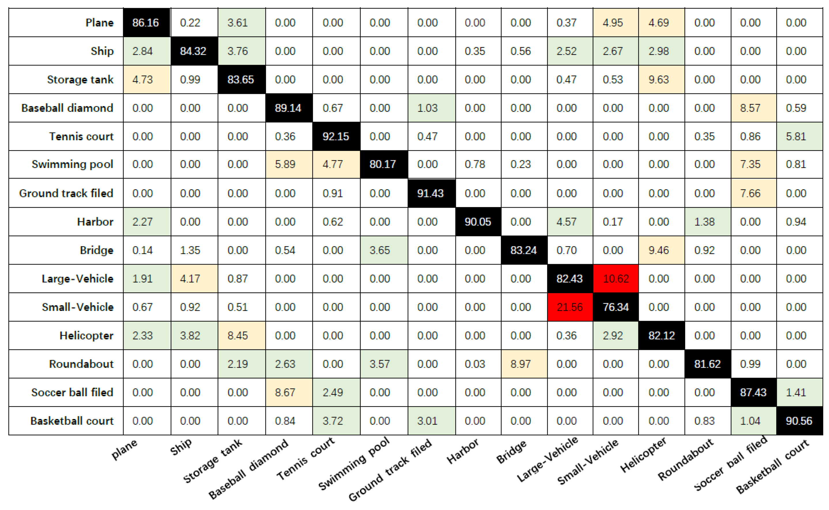
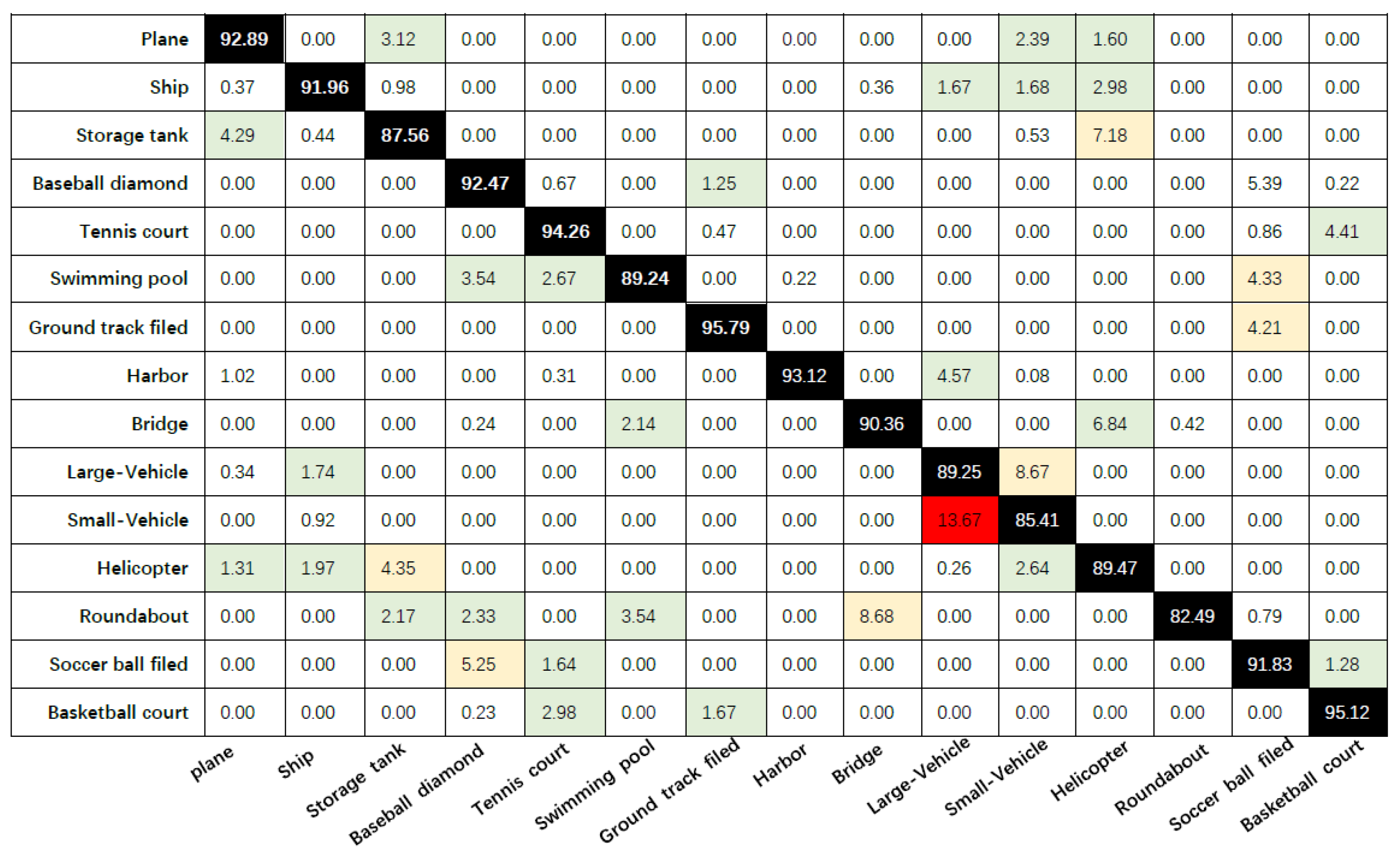
We further analyze the confusion matrix with the auxiliary network YOLOv3 and the improved model in this paper to evaluate the detection performance of the model. Figure 9 and Figure 10 represent the confusion matrix with the auxiliary network YOLOv3 and the confusion matrix of the model in this paper, respectively. The average detection accuracies (corresponding to the average results of the diagonal elements) of “YOLOv3 with auxiliary network” and “the methods in this paper” are 85.39% and 90.75%, respectively. According to the results of the confusion matrix, our model outperforms the model with the auxiliary network YOLOv3 for every type of target in the DOTA dataset, especially for the relatively small targets “Plane”, “Ship”, “Large-Vehicle” and “Small-Vehicle”.
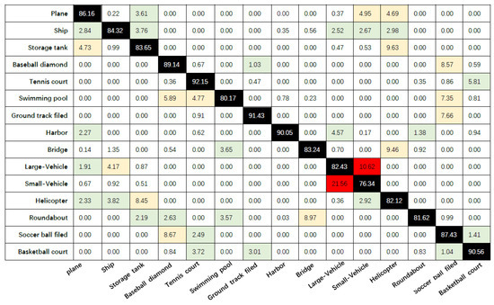
Figure 9.
Confusion matrix for YOLOv3 with auxiliary network.
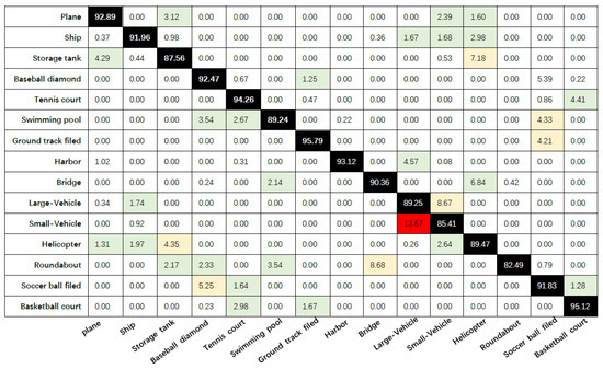
Figure 10.
Confusion matrix for the methods in this paper.
Taking YOLOv3 as the baseline for comparison, the original YOLOv3 mAP is only 79.19%, and the mAP of the YOLOv3 model with auxiliary network based on this article is 85.39%. In summary, the mAP of our improved YOLOv3 model is 2.49% higher than the mAP of Faster R-CNN, the best performing two-stage algorithm. This article serves as a reference benchmark for the YOLOv3 model with an auxiliary network. The mAP of the method used in this article is increased by 5.36%. The Our-Yolo network tested and compared with typical networks at one-stage and two-stage. Using the DOTA dataset to test and compare the average accuracy and processing speed. The comparison results are shown in Table 3.
Table 3.
Comparison of detection frame rates and standard deviations on the DOTA dataset (%).
As seen in Table 3, the mAP and detection speed of our model are higher than both two-stage Faster R-CNN and Fast R-CNN target detection algorithms.
Compared with the original YOLOv3(Darknet53), mAP has been greatly improved at the expense of detection speed. Compared with YOLOv3 (Auxiliary Network), our model not only improves the accuracy, but also slightly improves the speed.
Finally, comparing OUR-YOLOv3 (without ASFF) and OUR-YOLOv3 was deployed ASFF, the detection speed of the network model deployed with ASFF has been improved.
For evaluating a target detection model, it is necessary to compare the effectiveness of the model for inter class detection. Therefore, we introduce standard deviations to compare the detection effectiveness of the models for detecting targets between classes. As shown in Table 3, YOLOv3, Faster R-CNN, and Fast R-CNN have the highest standard deviation, which is due to the fact that these three models have good results for detecting large targets but for small targets, such as those occupying only 10–50 pixels, the detection is not as good and therefore results in a relatively large difference between classes. For our improved model, the standard deviation is the lowest, with a smaller gap than the inter class gap with the auxiliary network YOLOv3. It was demonstrated that our model can detect different classes of targets very well; in other words, our model does not differ much for the detection of different classes of targets.
As shown in Table 4, DIou loss can improve the performance with gains of 3.77%AP and 5.05%AP75 using GIoU as the evaluation metric.
Table 4.
Quantitative comparison of YOLOv3 (improved method in this article) trained using (baseline), and . The results are reported on the test set of DOTA.
The errors of TOP-1 and TOP-5 are shown in Table 5; the Top-1 error rate of CBAM deployed in our YOLOv3 is 1.25% lower than the Top-1 error rate of using the SE attention mechanism. The Top-5 error rate of CBAM deployed in our YOLOv3 is 0.6% lower than the Top-5 error rate of using the SE attention mechanism. It can be proved that CBAM will obtain better results than SE.
Table 5.
The YOLOv3 improved in this paper deployed the SE attention mechanism and CBAM respectively, and compares the error of Top-1 and Top-5.
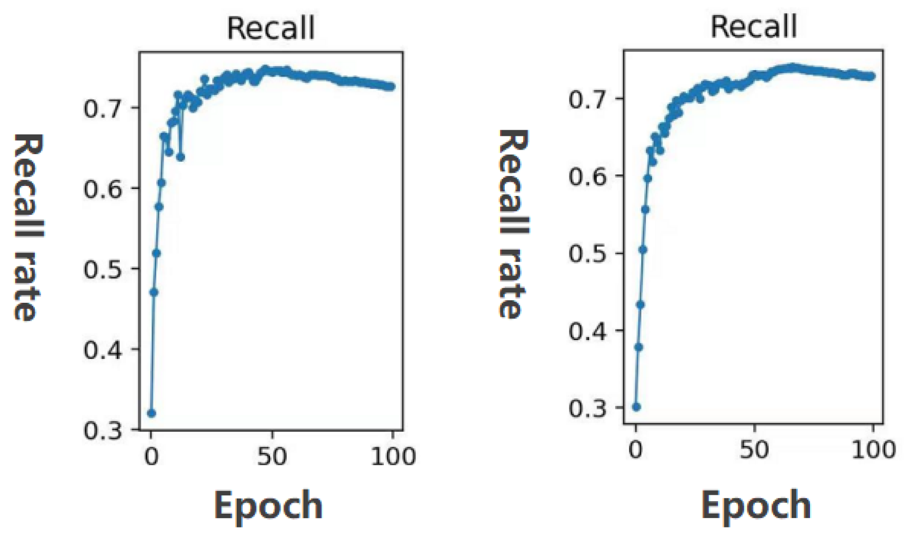
To further compare the recall rate, the comparison result is shown in Figure 11. It can be seen from Figure 11 that the improved YOLOv3 model has a higher recall rate than the YOLOv3 with an auxiliary network. Therefore, the method used in this article is more accurate than the YOLOv3 with an auxiliary network.

Figure 11.
Recall comparison between YOLOv3 with auxiliary network and the method in this paper. The recall of the YOLOv3 model with auxiliary network on the left, and the recall of the improved model in this paper on the right. (The horizontal coordinate is the number of epochs and the vertical coordinate is the recall rate).
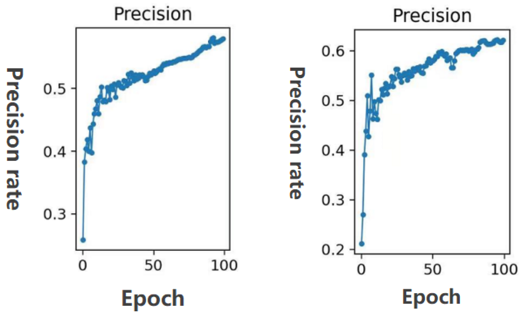
Figure 12 shows the comparison of the precision rate. It can be clearly seen from the figure that the method used in this article has a higher precision rate.
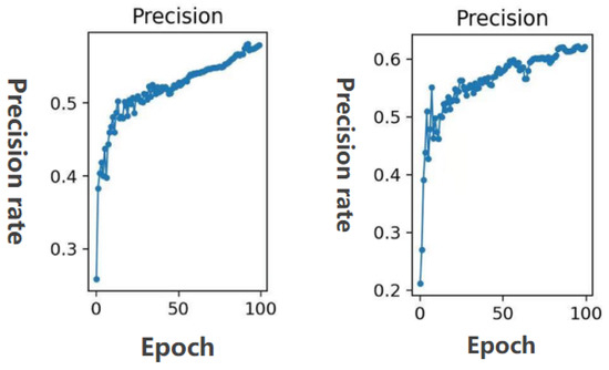
Figure 12.
Precision comparison between YOLOv3 with auxiliary network and the method in this paper.The precision of the YOLOv3 model with auxiliary network on the left, and the precision of the improved model in this paper on the right. (The horizontal coordinate is the number of epochs and the vertical coordinate is the precision rate).
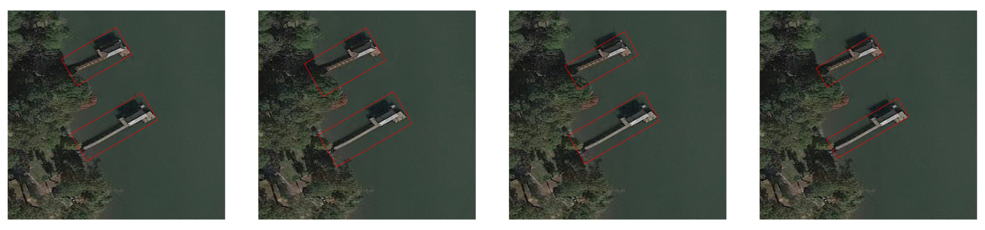
3.3. Qualitative Results and Analysis of the Bounding Box
This section presents a qualitative analysis of the Bounding Box for different network models (Faster R-CNN, YOLOv3, YOLOv3 with auxiliary network, and our YOLOv3). As shown in Figure 13, it is clear from the four figures above that the Bounding Box regression of the Faster R-CNN is better than that of YOLOv3, and it is clear from the figure that the Bounding box of YOLOv3 does not completely frame the target. The back of the harbor in the figure has a shaded part, but the shaded part is not needed. The Bounding Box of YOLOv3 with the auxiliary network excludes some of the shadows from the box, but the Faster R-CNN has all the shadows in the box, so the Bounding Box of YOLOv3 with the auxiliary network has better regression results. Finally, comparing the Bounding Box of YOLOv3 with the auxiliary network with our model, the Bounding Box of our model excluded the shadows very well. This example is a good illustration of how our model’s bounding box regression works better.
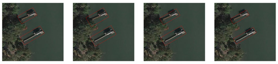
Figure 13.
Qualitative results for Bounding Box.
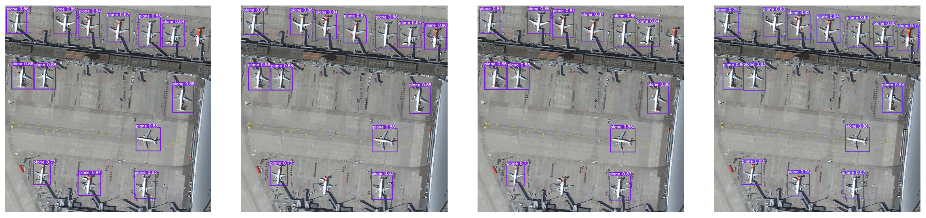
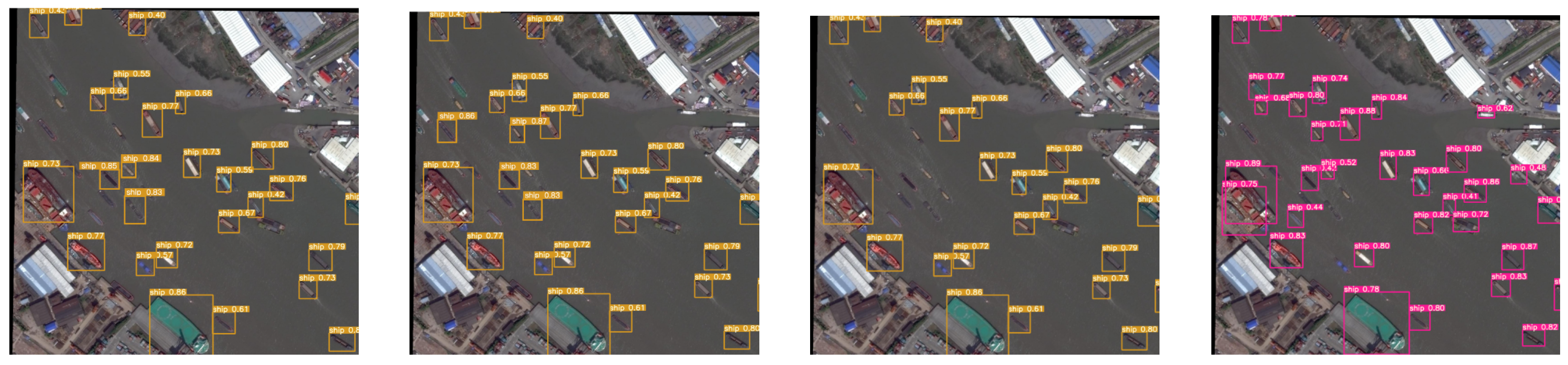
3.4. Detection Effect and Analysis
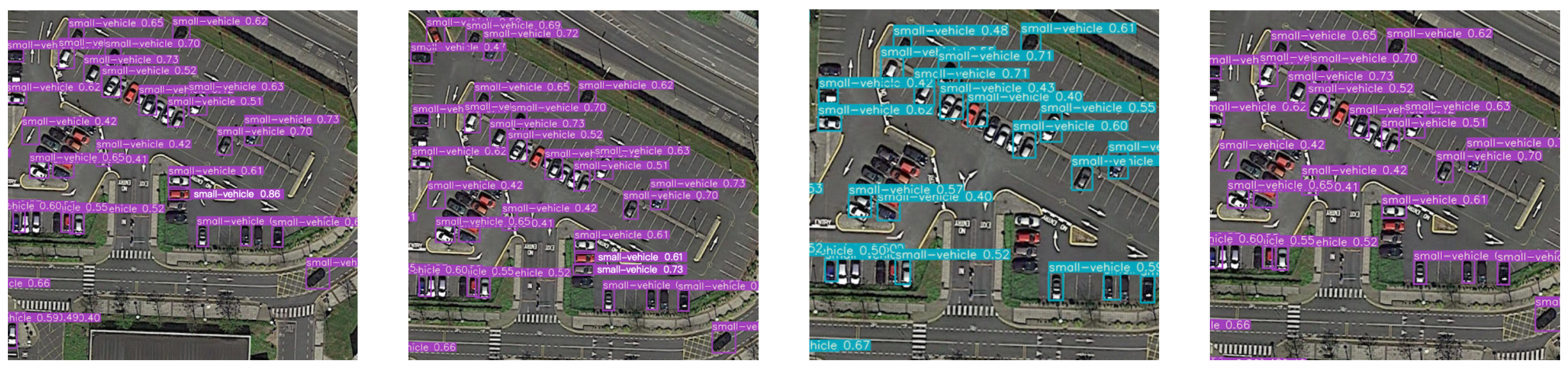
In this experiment, we made 50 control groups of effects, but the space of the article is limited to using only three of them as our effect demonstration. As shown in Figure 14, Figure 15 and Figure 16, each group of images from left to right shows the detection effect of Fast R-CNN, Faster R-CNN, YOLOv3 with auxiliary network and the improved method in this paper, respectively. It can be seen that the detection effect of our improved YOLOv3 model is better than the other three models (Faster R-CNN, Fast R-CNN, YOLOv3 with auxiliary network). Specifically, taking Figure 14 as an example, Faster R-CNN and Fast R-CNN missed a plane, respectively. The YOLOv3 model with an auxiliary network missed two planes. The YOLOv3 model we designed can detect the plane that the other three models missed.
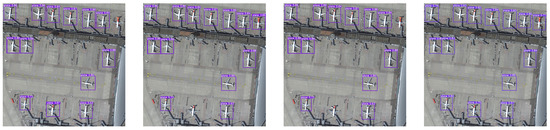
Figure 14.
The first group effect is shown.

Figure 15.
The second group effect is shown.

Figure 16.
The third group effect is shown.
4. Conclusions
The focus of this paper is on the application of auxiliary networks to remote sensing image target detection and the improvement of YOLOv3 with auxiliary networks. Our main work and improvements are as follows. Firstly, since the YOLOv3 network can only handle fixed size images due to the varying size of remote sensing images, we add an image blocking module to the input of the YOLOv3 model to crop the images to a fixed size for subsequent input to the network. Then, to make feature extraction more adequate, we changed the SE attention mechanism used in the YOLOv3 model with the auxiliary network to a convolutional block attention module, which makes it easier to obtain the features we need after feature extraction, and enhances the feature extraction capability of the network. After that, we use an adaptive feature fusion structure to replace the original feature pyramid structure. This approach not only solves the problem of insufficient feature fusion, but also makes our model more robust. Finally, to speed up the training of the network, a more efficient DIoU loss function is used.
In the experimental part, we conducted a large number of controlled experiments, as shown in Table 2. We compared the mAP of the method in this paper with the mAP of two-stage and one-stage; the mAP of our model was higher than that of all the algorithmic models involved in the comparison, which proves that our model makes some improvement in detection accuracy. We further provide the confusion matrix for YOLOv3 with the auxiliary network and the confusion matrix for the method in this paper, which show more intuitively that our network has a good improvement in the accuracy of “Plane”, “Ship”, “Large-vehicle”, and “Small-vehicle”, which are relatively small targets. Because we introduced an adaptive feature fusion approach, the problem of slower detection caused by the increase in the number of layers of the YOLOv3 network with auxiliary networks was also improved, and the results are shown in Figure 3. To demonstrate the superiority of DIoU loss, as shown in Table 4, we compared DIoU with IoU and GIoU, and successfully demonstrated the superiority of the DIoU loss function based on the AP and AP75 that we obtained. In order to demonstrate the effectiveness of adding CBAM, as shown in Table 5, we compared the addition of the SE attention mechanism to our model with the CBAM error rate, respectively, and demonstrated that the performance of our model was improved by CBAM based on the TOP-1 and TOP-5 we obtained. The recall as well as the accuracy rates of YOLOv3 with the auxiliary network and the method in this paper are given in Figure 11 and Figure 12, and show that our model has better data results under the same epoch. In Figure 13, the qualitative analysis of the Bounding Box obtained by Faster R-CNN, YOLOv3, YOLOv3 with auxiliary networks and the method in this paper is presented, and it can be seen that our method had a more accurate Bounding Box. We show our results in Figure 14, Figure 15 and Figure 16 and discuss the results obtained, which show a very intuitive improvement in the detection performance of our method.
We validated our model on the DOTA dataset and proved the robustness of our model. mAP improved by 5.36% over the YOLOv3 model with the auxiliary network and the frame rate improved by 3.07 FPS over the YOLOv3 model with the auxiliary network. As the improvement in detection speed in this paper is not significant enough, the main direction of future research is to reduce the detection time.
Author Contributions
Conceptualization, Z.Q. and F.Z.; methodology, Z.Q. and F.Z.; writing—original draft preparation, Z.Q.; writing—review and editing, F.Z. and C.Q.; supervision, F.Z.; funding acquisition, F.Z. All authors have read and agreed to the published version of the manuscript.
Funding
This work is supported in part by the National Natural Science Foundation China (61601174), in part by the Postdoctoral Research Foundation of Heilongjiang Province (LBH-Q17150), in part by the Science and Technology Innovative Research Team in Higher Educational Institutions of Heilongjiang Province (No. 2012TD007), in part by the Fundamental Research Funds for the Heilongjiang Provincial Universities (KJCXZD201703) and in part by the Science Foundation of Heilongjiang Province of China (F2018026).
Institutional Review Board Statement
Not applicable.
Informed Consent Statement
Not applicable.
Data Availability Statement
Data used in this study are available from corresponding authors by request.
Conflicts of Interest
The authors declare no conflict of interest.
Abbreviations
The following abbreviations are used in this manuscript:
| RSI | Remote Sensing Image |
| CBAM | Convolutional Block Attention Module |
| CNN | Convolutional Neural Network |
| MLP | Multi-layer perceptrons |
| ASFF | Asaptive Feature Fusion |
References
- Cheng, G.; Han, J. A survey on object detection in optical remote sensing images. ISPRS J. Photogram. Remote Sens. 2016, 117, 11–28. [Google Scholar] [CrossRef] [Green Version]
- Li, K.; Wan, G.; Cheng, G.; Meng, L.; Han, J. Object detection in optical remote sensing images: A survey and a new benchmark. ISPRS J. Photogram. Remote Sens. 2020, 159, 296–307. [Google Scholar] [CrossRef]
- Long, J.; Shelhamer, E.; Darrell, T. Fully convolutional networks for semantic segmentation. In Proceedings of the IEEE Conference on Computer Vision and Pattern Recognition, Honolulu, HI, USA, 21–26 July 2017; pp. 4700–4708. [Google Scholar]
- Wang, Q.; Gao, J.; Li, X. Weakly supervised adversarial domain adaptation for semantic segmentation in urban scenes. IEEE Trans. Image Process. 2019, 28, 4376–4386. [Google Scholar] [CrossRef] [PubMed] [Green Version]
- He, K.; Zhang, X.; Ren, S.; Sun, J. Deep residual learning for image recognition. In Proceedings of the IEEE Conference on Computer Vision and Pattern Recognition, Las Vegas, NV, USA, 27–30 June 2016; pp. 770–778. [Google Scholar]
- Huang, G.; Liu, Z.; Van Der Maatten, L.; Weinberger, K.Q. Densely connected convolutional networks. In Proceedings of the IEEE Conference on Computer Vision and Pattern Recognition, Honolulu, HI, USA, 21–26 July 2017; pp. 4700–4708. [Google Scholar]
- Girshick, R. Fast R-CNN. In Proceedings of the IEEE International Conference on Computer Vision ( ICCV), Santiago, Chile, 13–16 December 2015; pp. 1440–1448. [Google Scholar]
- Hu, Y.; Li, X.; Zhou, N.; Yang, L.; Peng, L.; Xiao, S. A sample update-based convolutional neural network framework for object detection in large-area remote sensing images. IEEE Geosci. Remote Sens. Lett. 2019, 16, 947–951. [Google Scholar] [CrossRef]
- Yoo, J.J.; Ahn, N.H.; Sohn, K.A. Rethinking Data Augmentation for Image Super-Resolution: A Comprehensive Analysis and a New Strategy. Available online: https://arxiv.org/abs/2004.00448 (accessed on 23 April 2020).
- Girshick, R.; Donahue, J.; Darrell, T. Rich feature hierarchies for accurate object detection and semantic segmentation. In Proceedings of the IEEE Conference on Computer Vision and Pattern Recognition (CVPR), Columbus, OH, USA, 23–28 June 2014; pp. 580–587. [Google Scholar]
- Ren, S.; He, K.; Girshick, R. Faster R-CNN: Towards Real-Time Object Detection with Region Proposal Networks. IEEE Trans. Pattern Anal. Mach. Intell. 2017, 39, 1137–1149. [Google Scholar] [CrossRef] [Green Version]
- He, K.; Gkioxari, G.; Dolloor, P.; Girshick, R. Mask R-CNN. In Proceedings of the IEEE Conference on Computer Vision and Pattern Recognition, Honolulu, HI, USA, 21–26 July 2017; pp. 2961–2969.
- Redmon, J.; Divvala, S.; Girshick, R. You Only Look Once: Unified, Real-Time Object Detection. In Proceedings of the IEEE International Conference on Computer Vision (ICCV), Las Vegas, NV, USA, 27–30 June 2016; pp. 1063–6919. [Google Scholar]
- Redmon, J.; Farhadi, A. YOLO9000: Better, Faster, Stronger. In Proceedings of the IEEE Conference on Computer Vision and Pattern Recognition, Honolulu, HI, USA, 21–26 July 2017; pp. 7263–7271. [Google Scholar]
- Redmon, J. YOLOv3: An Incremental Improvement. Available online: https://arxiv.org/abs/1804.02767 (accessed on 8 April 2018).
- Lin, T.Y.; Dolloor, P.; Girshick, R.; He, K.; Hariharan, B.; Belongie, S. Feature pyramid networks for object detection. In Proceedings of the IEEE Conference on Computer Vision and Pattern Recognition, Honolulu, HI, USA, 21–26 July 2017; pp. 2117–2125. [Google Scholar]
- Vinyals, O.; Blundell, C.; Lillicrap, T.; Kavukcuoglu, K.; Wierstra, D. Matching networks for one shot learning. Proc. Adv. Neural Inf. Process. Syst. 2016, 10, 3630–3638. [Google Scholar]
- Dai, Z.G.; Cai, B.L.; Lin, Y.G.; Chen, J.Y. UP-DETR: Unsupervised Pre-Training for Object Detection with Transformers. Available online: https://arxiv.org/abs/2011.09094 (accessed on 7 April 2021).
- Volpi, M.; Morsier, F.D.; Camps-Valls, G.; Kanevski, M.; Tuia, D. Multi-sensor change detection based on nonlinear canonical correlations. In Proceedings of the 2013 IEEE International Geoscience and Remote Sensing Symposium-IGARSS, Melbourne, VIC, Australia, 21–26 July 2013; pp. 1944–1947. [Google Scholar]
- Bai, X.; Zhang, H.; Hou, J. VHR object detection based on structural feature extraction and query expansion. IEEE Trans. Geosci. Remote Sens. 2014, 10, 6508–6520. [Google Scholar]
- Bi, F.; Zhu, B.; Gao, L.; Bian, M. A visual search inspired computational model for ship detection in optical satellite images. IEEE Geosci. Remote Sens. Lett. 2012, 9, 749–753. [Google Scholar]
- Huang, X.; Zhang, L. Road centreline extraction from high-resolution imagery based on multiscale structural features and support vector machines. Int. J Remote Sens. 2009, 30, 1977–1987. [Google Scholar] [CrossRef]
- Cheng, G.; Zhou, P.; Han, J. Learning rotation-invariant convolutional neural networks for object detection in VHR optical remote sensing images. IEEE Trans. Geosci. Remote Sens. 2016, 54, 7405–7415. [Google Scholar] [CrossRef]
- Zhang, Y.; Yuan, Y.; Feng, Y.; Lu, X. Hierarchical and robust convolutional neural network for very high-resolution remote sensing object detection. IEEE Trans. Geosci. Remote Sens. 2019, 57, 5535–5548. [Google Scholar] [CrossRef]
- Li, K.; Cheng, G.; Bu, S.; You, X. Rotation insensitive and context augmented object detection in remote sensing images. IEEE Trans Geosci. Remote Sens. 2018, 56, 2337–2348. [Google Scholar] [CrossRef]
- Tang, T.; Zhou, S.; Deng, Z.; Zou, H.; Lei, L. Vehicle detection in aerial images based on region convolutional neural networks and hard negative example mining. Sensors 2017, 17, 336. [Google Scholar] [CrossRef] [PubMed] [Green Version]
- Zou, Z.; Shi, Z. Ship detection in spaceborne optical image with SVD networks. IEEE Trans. Geosci. Remote Sens. 2016, 54, 5832–5845. [Google Scholar] [CrossRef]
- Lin, H.; Shi, Z.; Zou, Z. Fully convolutional network with task partitioning for inshore ship detection in optical remote sensing images. IEEE Geosci. Remote Sens. Lett. 2017, 14, 1665–1669. [Google Scholar] [CrossRef]
- Liu, W.; Ma, L.; Chen, H. Arbitrary oriented ship detection frame-work in optical remote sensing images. IEEE Geosci. Remote Sens. Lett. 2018, 15, 937–941. [Google Scholar] [CrossRef]
- Tang, T.; Zhou, S.; Deng, Z.; Lei, L.; Zou, H. Arbitrary oriented vehicle detection in aerial imagery with single convolutional neural networks. Remote Sens. 2017, 9, 1170. [Google Scholar] [CrossRef] [Green Version]
- Liu, L.; Pan, Z.; Lei, B. Learning a rotation invariant detector with rotatable bounding box. IEEE Geosci. Remote Sens. Lett. 2017, 9, 960. [Google Scholar]
- Liu, W. SSD: Single Shot MultiBox Detector. In European Conference on Computer Vision; Springer: Cham, Switzerland, 2016; pp. 21–37. [Google Scholar]
- Zhong, J.; Lei, T.; Yao, G. Robust vehicle detection in aerial images based on cascaded convolutional neural networks. Sensors 2017, 17, 2720. [Google Scholar] [CrossRef] [Green Version]
- Han, X.; Zhong, Y.; Zhang, L. An efficient and robust integrated geospatical object detection framework for high spatial resolution remote geospatial sensing imagery. Remote Sens. 2017, 9, 666. [Google Scholar] [CrossRef] [Green Version]
- Xu, Z.; Xu, X.; Wang, L.; Yang, R.; Pu, F. Deformable ConvNet with aspect ratio constrained NMS for object detection in remote sensing imagery. Remote Sens. 2017, 9, 1312. [Google Scholar] [CrossRef] [Green Version]
- Xun, Q.W.; Lin, R.Z.; Yue, H.; Huang, H. Research on Small Target Detection in Driving Scenarios Based on Improved Yolo Network. IEEE Access 2019, 8, 27574–27583. [Google Scholar]
- Woo, S.; Park, J.; Lee, J.Y. CBAM: Convolutional Block Attention Module; Springer: Cham, Switzerland, 2018; p. 112211. [Google Scholar]
- Liu, S.; Huang, D.; Wang, Y. Learning Spatial Fusion for Single-Shot Object Detection. Available online: https://arxiv.org/abs/1911.09516 (accessed on 21 September 2019).
- Zheng, Z.; Wang, P.; Liu, W. Distance-IoU Loss: Faster and Better Learning for Bounding Box Regression. Proc. AAAI Conf. Artif. Intell. 2020, 34, 12993–13000. [Google Scholar] [CrossRef]

Publisher’s Note: MDPI stays neutral with regard to jurisdictional claims in published maps and institutional affiliations. |
© 2021 by the authors. Licensee MDPI, Basel, Switzerland. This article is an open access article distributed under the terms and conditions of the Creative Commons Attribution (CC BY) license (https://creativecommons.org/licenses/by/4.0/).