Article

3D Point Cloud Semantic Augmentation: Instance Segmentation of 360° Panoramas by Deep Learning Techniques

1
College of Geomatic Sciences and Surveying Engineering, Institute of Agronomy and Veterinary Medicine, Rabat 10112, Morocco
2
Geomatics Unit, University of Liège (ULiège), 4000 Liège, Belgium
*
Author to whom correspondence should be addressed.
Remote Sens. 2021, 13(18), 3647; https://doi.org/10.3390/rs13183647
Submission received: 20 July 2021 / Revised: 30 August 2021 / Accepted: 31 August 2021 / Published: 13 September 2021
(This article belongs to the Special Issue 3D Indoor Mapping and BIM Reconstruction)

Abstract

:
Semantic augmentation of 3D point clouds is a challenging problem with numerous real-world applications. While deep learning has revolutionised image segmentation and classification, its impact on point cloud is an active research field. In this paper, we propose an instance segmentation and augmentation of 3D point clouds using deep learning architectures. We show the potential of an indirect approach using 2D images and a Mask R-CNN (Region-Based Convolution Neural Network). Our method consists of four core steps. We first project the point cloud onto panoramic 2D images using three types of projections: spherical, cylindrical, and cubic. Next, we homogenise the resulting images to correct the artefacts and the empty pixels to be comparable to images available in common training libraries. These images are then used as input to the Mask R-CNN neural network, designed for 2D instance segmentation. Finally, the obtained predictions are reprojected to the point cloud to obtain the segmentation results. We link the results to a context-aware neural network to augment the semantics. Several tests were performed on different datasets to test the adequacy of the method and its potential for generalisation. The developed algorithm uses only the attributes X, Y, Z, and a projection centre (virtual camera) position as inputs.

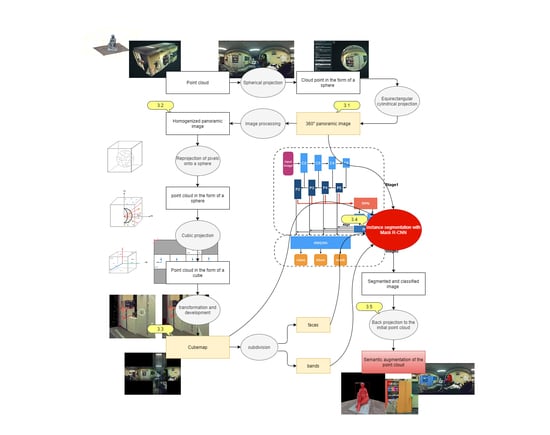
Graphical Abstract

1. Introduction

Understanding and interpreting complex 3D scenes is an innate human visual task that can be performed instantaneously and effortlessly. Delegating this task to the machine is a significant challenge that has attracted several researchers from various disciplines. Transforming a human-centred process into a fully “artificial” workflow requires one to deeply investigate automation processes and Artificial Intelligence (AI) algorithms that can permit human-like inference.
This is particularly crucial for the better integration of point clouds in 3D capture workflows, where objects, described by sets of points, primarily need to be clearly identified [1]. Furthermore, the manual segmentation of datasets composed of billions of points is extremely cumbersome and imprecise, and workflows with a high level of automation are highly sought after. The research community is investigating state-of-the-art supervised learning methods, but the lack of available 3D point cloud training datasets is a major hurdle [2]. Moreover, direct automation through Deep Learning (DL) methods presents many difficulties for semantic segmentation tasks; the most obvious of which is the size of the data itself. Another hurdle is the lack of clear structure akin to the regular grid arrangement in images [3]. Finally, in the interest of generalisation, the number of supported classes is often in the range of 1–10 and cannot reasonably scale to the various domain definition needs. These obstacles have likely prevented Convolutional Neural Networks (CNNs) from achieving the impressive performances attained for regular datasets such as speech processing or images, using irregular data [4].
This research aims to overcome the challenges by adopting an inverse approach for point cloud semantic augmentation using an instance segmentation technique. We propose to leverage complete and robust deep learning models that can detect many objects. In fact, the method investigates the exploitation of pre-established image datasets to solve the problem of insufficient data concerning point clouds. In addition, we hypothesise that projecting a point cloud into an image has the advantage of extending all the research carried out over the last decade on 2D images to 3D point clouds [5], especially the robust neural networks for object detection, semantic segmentation, and instance segmentation in 2D data (FCN [6]; the R-CNN series: R-CNN [7], Fast R-CNN [8], Faster R-CNN [9], Mask R-CNN [10]; YOLO [11]).
Traditionally, two categories of methods were commonly used to segment images: pixel-based classifiers and Object-Based Image Analysis (OBIA) [12], and that, especially in the field of remotely sensed imagery, captured by satellites, airplanes, or drones. Only the spectral information available for each pixel is used in pixel-based methods. They are faster but ineffective in some cases, particularly for high-resolution images and heterogeneous object detection ([13,14,15]). Object-based methods take into account the spectral as well as the spatial properties of image segments (a set of similar neighbour pixels). OBIA-methods represent the state-of-the art in remote sensing for object detection [16], high-resolution land-cover mapping ([17,18]), and change detection [19]. However, contrary to deep learning techniques, OBIA-based models are not learnable models: they cannot learn from an image and reutilize the learning into another. The detection is performed from scratch on each new individual image [13].
This paper is organised as follows: In Section 2, we review the related work, guidelines, and definitions, of the current study. Section 3 gives the proposed method providing details about the projection and the deep learning parts. In Section 4, we explain the details about experimental results. Section 5 provides the general discussion. Finally, we conclude in Section 6.

2. State of the Art/Overview

This section briefly introduces the different concepts that are either used or related to this study and thus necessary for its understanding. We organise the related works into the two following sections: Section 2.1 includes the definition of panoramic images and geometric projections that encompass a big part of the current research; Section 2.2 describes the different deep learning semantic extraction techniques in computer vision. In this same section, we give a brief cover of Tabkha’s thesis [20], which preceded this research.

2.1. Panoramic Image and Projections

Panoramic photography is very diverse. For some “panoramists”, it is a photo in elongated format. For others, the elongated format is not sufficient; the image must also embrace a wide angle of view that exceeds a certain threshold [21]. The most common definition of a panoramic image is the image that covers the entire surrounding space [22]; consequently, a cubemap is also considered as a panoramic image even if it presents a less homogeneous rendering due to the dissociation into six distinct images. Note all the same that this definition remains questionable and is still the subject of a long debate.
The creation of panoramic images necessarily requires the passage through the notion of geometric projections. Each type of projection gives a different degree and type of distortion which returns a very special visual signature. Today, there are three main categories and a multitude of types.
These three categories are: rectilinear projections, curved or tiled projections, and unique projections.

2.1.1. Rectilinear Projection

This projection produces classic panoramas while maintaining straight and vertical lines (any straight line in the real world is displayed as a straight line in the panorama; this makes it a suitable projection for architectural panoramas), which is the type of projection that regular images have: a conical perspective projection on a projection plane. With this type of projection, all of the projection lines converge towards the same point O called the centre of projection, and the projection lines form a cone, hence the name “conical projection” [23].
The cubic projection is mainly used for virtual tour and panorama creation applications. Its approach consists of projecting a 3D scene (in a classical perspective projection) from the centre of the cube through the six facets’ directions and then flattening the cube by developing it on a flat surface. This representation is less homogeneous than the spherical and cylindrical projection since it introduces discontinuities at the level of each edge of the projection cube. The cubic projection offers the advantage of covering the entire surrounding space and the absence of the curved line type distortions generated by spherical and cylindrical projections. Therefore, each facet of the cubemap resembles an image taken by a normal camera (rectilinear projection), which is why we have adopted this type of projection in this project to better result from object detection by the neural network.
We can consider that the cubic projection is within the rectilinear projection category since each facet of the cubemap represents the rectilinear projection of a portion of the space surrounding one of the cube planes; in total, there are six rectilinear projections on the six plane surfaces of the cube.

2.1.2. Curved or Tiled Projection

As its name implies, this projection generates deformations of straight lines that become more curved as one moves away from the central horizontal line of the panoramic image (all vertical straight lines are kept, but the horizontals lines become curved except for the horizon line). This is the case of cylindrical and spherical projections [21].
The spherical projection consists of projecting the points of the surrounding space onto a sphere of diameter R and centre O. The projected points result from the intersection of the lines connecting the points from the cloud to the centre of the sphere. The spherical projection has the advantage of being able to represent the totality of the surrounding space. In addition, this representation is more homogeneous than the cubic projection since each direction is represented in an equivalent way and without discontinuities. The main drawback of this projection is that it is not directly developable on a plane. To avoid this problem, it is essential to introduce another type of projection as in the case of cartographic projections where it is necessary, to produce a map, to project the earth (sphere/ellipsoid) onto a cone (conical projection), a plane (azimuthal projection), a cylinder (cylindrical projection, Mercator), etc.
The cylindrical projection is one of the most famous projections in the history of mapping. This involves projecting the earth onto a normal, transverse, or oblique cylinder, then develop it on a flat surface. The meridians are represented by equidistant parallel lines, and parallels are represented by lines perpendicular to the images of the meridians but at varying distances depending on the type of cylindrical projection. In fact, it is the grid of parallels that differentiates the different cylindrical projections. In the cylindrical Mercator projection, for example, meridians are equally spaced vertical lines, and parallels of latitude are straight horizontal lines that are spaced farther apart from the equator [24]. The Mercator projection is conformal (preserves angles and shapes) [25].
In the present work, to generate the panoramic image, we have adopted the equirectangular projection, also called equidistant cylindrical projection or plane chart, and this, for the simple reason that it is the easiest to translate into image format (pixels), because it converts a sphere into a Cartesian grid. In addition, its field of vision is not limited (360° × 180°), and it is the most used projection for this type of transformation (by stitching software and some cameras). Unlike the Mercator projection, the equirectangular projection generates, in the case of a cartographic projection, meridians projected onto equally spaced vertical lines and parallels projected onto equidistant horizontal lines. This projection is neither conformal nor equivalent, which explains its absence on navigation charts and topographic maps. However, it is particularly used for generating panoramic raster images from a sphere, and it comes down to the simple relationship between the position of a pixel in the panoramic image and its corresponding location on the sphere in spherical coordinates. In fact, the horizontal coordinate is simply longitude on the panoramic image, and the vertical coordinate is simply latitude [26]. The poles (zenith, nadir) of the sphere are located at the top and bottom of the image and are stretched across the image’s width. The areas near the poles are also stretched horizontally, which implies a very large number of data redundancy near the poles [27]. The panoramic image by equirectangular projection must have a length/width ratio equal to 2:1, since it represents an angle of 0–360° in width (longitude) and an angle of 0–180° in height (latitude).

2.1.3. Special Projection

They come in several variants: the Panini projection [28], the Mini planet projection [29], the Hammer projection, the Mirror Ball projection [30], the orthographic projection, etc. The Mini planet projection, also called the stereographic projection, is the most famous of them, especially among enthusiasts of panoramic photography. Initially, this projection’s principle consists of bringing together camera shots into a 360° panoramic image. Subsequently, it is a question of projecting the information of the panoramic image on a sphere, and finally to obtain a plane representation with the “mini planet” effect, it is necessary to project the sphere on an azimuthal plane, hence the name stereographic projection. The projection of a point represents the intersection with the azimuthal projection plane considered (for example the plane z = −1), of the line which links this point to the North Pole of the sphere.
In the present work, we used the cylindrical, spherical, and cubic projections that were applied on the point clouds to produce panoramic images.

2.2. Segmentation for the Extraction of Semantics

DL has become the most powerful tool for data processing in computer vision, which is due to its powerful performance for tasks such as classification, segmentation, and detection [31] (Section 2.2.1, Section 2.2.2 and Section 2.2.3). While DL techniques are mainly used for data with a structured grid such as images, point cloud, on the other hand, comes with many challenges: occlusion, irregularity, and an unstructured and unordered data form. Regardless of the previous challenges, DL on raw point cloud is receiving lot of attention since PointNet [32] was released in 2017, which is based on two main symmetric functions, MultiLayer Perceptron (MLP) and a maxpooling function. The first stage consists of transforming the input raw point cloud using the previous two functions, to a feature vector (obtained in a winner-takes-all principal [33]), which represents the feature descriptor of the input that can be used for recognition and segmentation tasks in the second stage. Many state-of-the-art methods have been developed since then, such as PointNet++ [34] and RandLA-Net [35], which both rely on point-wise MLP. In addition, other networks such as PointCNN [36] and KPConv [37] are based on a point convolution method, as well as the graph-based networks such as DGCNN [38] and SuperPoint Graph (SPG) network [4].
Unlike point clouds format, images contain a regular, ordered, and structured data format, which is why we have chosen to test the efficiency of working in a 2D environment to semantically enrich a 3D point cloud. Therefore, the next sections focus on introducing DL techniques in a 2D context. There are several semantic extraction techniques in the field of computer vision: classification, object detection, semantic segmentation, and instance segmentation. The simplest of these is image classification, which tells us if one or more classes are present in the input image and returns several prediction values for each class.

2.2.1. Object Detection

Object detection is not limited to finding the classes of objects and detecting their positions on the image by bounding boxes. This type of technique is often used in self-driving car applications, since the car not only needs to know the classes of objects around it but also detect their positions to avoid them. Detection can be solved with a CNN network [39] followed by an FC network [40] but only in the case of images containing a single object, because in the case where there are multiple objects, the output length is unpredictable (unknown number of output parameters), knowing that in an object detection problem it is necessary to predict, in addition to the object class, the parameters of the bounding box (coordinates of the centre (bx, by), the height bh, and the width bw) [41].
To allow the detection of several objects with their bounding boxes, several neural network approaches have been developed ([8,9,11,42,43]); one of the most famous is the R-CNN approach [7]. This is a two-step detection: a Region of Interest (ROI) proposal step and a classification step. The general idea of the approach is to select different regions of interest in the image and to separately use a CNN in each of those regions. The advantage of this approach over others is that it adopts a maximum number of 2000 regions of interest based on a selective search (a fixed segmentation algorithm, which is not a neural network), which prevents over-segmentation of images. Therefore, instead of classifying a large number of regions, we can effectively work with only 2000 regions [7]. To improve this model, it is better to use a trainable algorithm in the form of a neural network for the detection of ROIs instead of using a fixed segmentation algorithm. Several improvements have been made recently to make the model faster as the Fast R-CNN model [8] and the Faster R-CNN model [9].

2.2.2. Semantic Segmentation

Semantic segmentation is a very popular technique in the field of computer vision. It is about understanding the image at the pixel level; this is a dense classification problem where each pixel of the input image is assigned to the class of the object that encompasses it. Therefore, it is clear that it is not a simple classification of the image but rather a dense classification at the pixel level, and the output image is fully segmented and classified.
The FCN (Fully Convolutional Network) [6] model created by Long et al. in 2015 is one of the most popular models to solve the problem of semantic segmentation. In fact, FCN is a neural network that consists only of convolutional layers, hence the name “Fully Convolutional Network”. It does not contain an FC network at the end as in the case of the usual CNN convolutional neural networks [6]. The FCN model is based mainly on two key operations: the Uppooling operation and the operation of merging the outputs of the intermediate convolutional layers.
The operation of pooling or subsampling induces a reduction in the size of the input image, thus, the names: Uppooling or Upsampling refer to the reverse operation which induces an increase in the size of the image in question. This operation is very important in the FCN model, because, in the end, we are looking to find the class predictions for each pixel of the input image, which means that we must have at the output a matrix (image) equal in resolution to the input image, containing predictions for each pixel in the image. However, the periodic operations of a CNN, “Max pooling” or “Average pooling”, considerably reduce the size of the initial image, all the more as we go deep into the network. However, to have a classification at the pixel level, the image at the output of the network must have the same size as the input image, hence the use of this type of operation at the end of the FCN network to find the size of the input image. The Uppooling operation is introduced after the detection of feature maps in the image.
The second key notion in an FCN is the merging of outputs. This is because convolutional networks begin to lose spatial information as they enter deep into the network, which boils down to decreasing the size of the images. Intermediate layers which are shallower contain more spatial information but, at the same time, a lower level of detected characteristics. Thus, the solution which has been adopted in the FCN model is to make a merge (addition element by element) between the layers which contain more spatial information about pixels (shallower layers) and layers that contain a high level of detected features (deep layers), as is the case of FCN-16s and FCN-8s [6].

2.2.3. Instance Segmentation

The technique of instance segmentation makes it possible to extract objects from images by assigning them to their appropriate classes, such that each pixel has the class of the enclosing object; therefore, it is a classification at the pixel level, but it should not be confused with the semantic segmentation technique, because here, only the objects of the image are classified at the pixel level and not the whole image. It is therefore a combination of the two object detection and semantic segmentation approaches [10]. The Mask R-CNN model, adopted in this study, is part of this category of segmentation techniques. The architecture of this model is detailed in the method section.

2.2.4. Previous Work: Tabkha’s Thesis 2019

To give a chronological order, this research follows Tabkha’s thesis [20], which was elaborated in 2019 under the title “Semantic Increase of a Point Cloud through the Automatic Extraction of a 360° Panorama and Its Integration into a Platform of Machine Learning ”.
The previous work that was carried out within this thesis is subdivided into three main parts. The first part concerns the creation of an image assimilating a (virtual) camera position within the point cloud by cylindrical panoramic projection with a width/height ratio equal to 2:1. As for the second part, specific image treatments were applied to the image to homogenise the rendering using median, statistical, and fill filters. Finally, the homogenised image was introduced into an open-source image recognition software using the Imagga API, which allows the tagging of images on “scalable clouds” via machine learning techniques.
The elaborated process is characterised by simplicity and automation, but the algorithm does not escape certain limits. There are several aspects to be improved, in particular the adoption of a panoramic projection, which allows the preservation of the whole cloud to thus avoid the loss of data of the points which are located above and below the projection cylinder. It is also preferable to break away from the Imagga API by developing a new approach to object recognition.

3. Methods

This section describes the point cloud analysis methodology used for semantic segmentation of a point cloud. Our automatic procedure is serialised in the steps shown in Figure 1. In Section 3.1, we describe the method of the constitution of the 360° panoramic image grid. Section 3.2 discusses the process followed to homogenise the renderings and thus enhance the classification step. Afterwards, in Section 3.3, we demonstrate the cubemap generation using a cubic projection. Section 3.4 explains the instance segmentation applied on the panoramic images using the Mask R-CNN neural network. Lastly, in Section 3.5, we present the back projection method of the predictions to the initial point cloud.

3.1. 360° Panoramic Image

3.1.1. Spherical Projection

Figure 2 shows the mathematical definition of the projection of a sphere with radius R and centre O (0, 0, 0). Considering the yellow point (P) with Cartesian coordinates (x, y, z), the problem consists in finding the Cartesian coordinates (x′, y′, z′) of the black point P′ which represents the intersection of the line connecting the point P to the centre of the sphere according to the known elements: x, y, z, and R, with D being the distance separating the centre of the sphere from the point P.
Based on Thales’s theorem, we obtain the following expression of P′ coordinates:
P ·   ( R x 2 + y 2 + z 2 × x ,     R x 2 + y 2 + z 2 × y ,     R x 2 + y 2 + z 2 × z ) ,
In the case of a point cloud, the sphere is not always located at the origin of the point cloud coordinate system, and it is therefore necessary to apply a translation of the centre of the sphere, before proceeding to the projection. For a better result, the sphere should be positioned inside the point cloud, putting its centre closer to the part that we want to highlight. To ensure the link between the projected points and those which correspond to them in the cloud, an identifier ‘i’ is added to the tables of the new coordinates of the points projected on the sphere, so that each point has a unique identifier throughout the whole development process.
The application of the spherical projection on a three-dimensional point cloud gives the following results (Figure 3).
The next step consists in projecting the sphere onto a cylinder using an equirectangular cylindrical projection in order to generate the 360° panoramic image.

3.1.2. Equirectangular Cylindrical Projection

This step consists of generating an equirectangular panoramic image from the projected points on the previous sphere. To accomplish this, it is necessary to calculate the image coordinates which correspond to each point projected on the sphere. In fact, there is a direct relation between the spherical coordinates of the points on the surface of the sphere and the image coordinates of the panoramic image after developing the cylinder of the equirectangular projection; more precisely, the horizontal coordinate on the panoramic image is the longitude, and the vertical coordinate is the latitude. It is important to note that this projection is neither conformal nor equivalent; it is particularly used to generate panoramic images.
We recall that the previously calculated coordinates of the points projected on the sphere are Cartesian coordinates. However, since the relationship between the spherical coordinates (r, φ, θ) and the image coordinates is the most obvious, we first transform the Cartesian coordinates of the points projected on the sphere into spherical coordinates. Then, considering the spherical coordinates of the point P′(r, φ, θ), its corresponding image coordinates (i, j) are calculated by the following equations:
i =   θ height π
j = φ width 2 π
The term (width) represents the desired number of columns on the panoramic image, and the term (height) represents the number of rows, both expressed in pixels. Which allows for the transforming of the points projected on the sphere to the image coordinates on the developed cylinder (Figure 4).
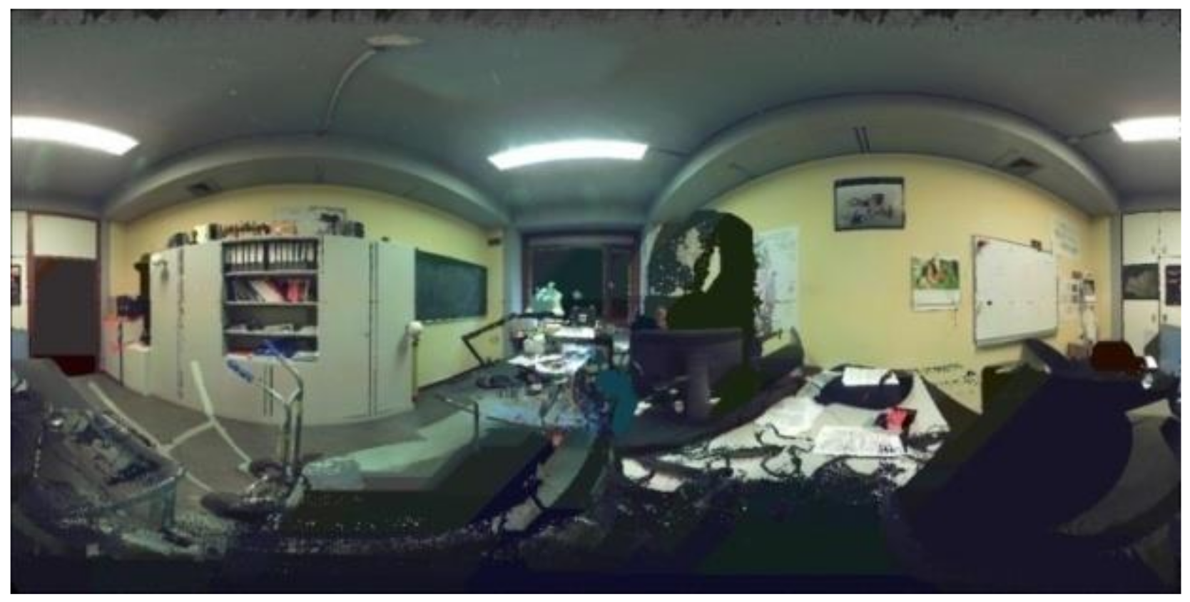
The panoramic image has been correctly generated; thus, the process is validated. Figure 5 shows the first generated panoramic image.
Based on the spherical projection of the points of the cloud, it is obvious that several projected points have the same coordinates (φ and θ). In fact, all the points of the cloud which are in the same line passing through the centre of the sphere have the same spherical coordinates. It is not the redundancies of the angles that are problematic but rather the question: which point is considered as the right point occupying the angle (φ, θ)?, since we later need its colour information (R, G, B) to generate the panoramic image. The correct point that should normally be considered is the closest point to the sphere’s centre, since logically, if we position ourselves inside the sphere we would only see the points that are in the foreground. The minimum distance condition is added to the code to keep only the right points representing the foreground view with respect to the virtual camera (centre of the sphere).

3.2. Homogenisation of the Panoramic Image

The panoramic image generated in the previous steps contains three major problems which are mainly related to the special nature of this generation: noise, empty areas, and artefacts related to the point cloud. In this part, we present the different filters adopted for reducing the three problems above while trying to keep the useful information contained in the image. The objective behind this homogenisation is to increase the rate of correct predictions in the instance segmentation part, since the neural network used is trained on a dataset containing normal images, which do not present these types of alterations. Of course, the use of a given filter is conditioned by the type of noise considered and by the intended use of the image subsequently (contour detection, segmentation, etc.)
We have chosen to apply homogenisation at this point and not after the generation of the second panoramic image (the cubemap) for the following reason: the cubemap itself presents a nonhomogeneous rendering with many empty areas resulting from the development of the cube on only six faces of the cubemap (the rest of the faces are empty and thus represented in black), and therefore, if we apply the filters on the cubemap, these empty areas would negatively influence the homogenisation result.
The first applied filter is the median filter which is generally used to eliminate salt and pepper noise [45]. This type of noise is very similar to the noise generated by empty pixels and point cloud artifacts on the panoramic image (Figures 20, 21 and 23), which is why it has been adopted. The good performance of the median filter stems from the property of the median to be almost insensitive to extreme pixel values [45].
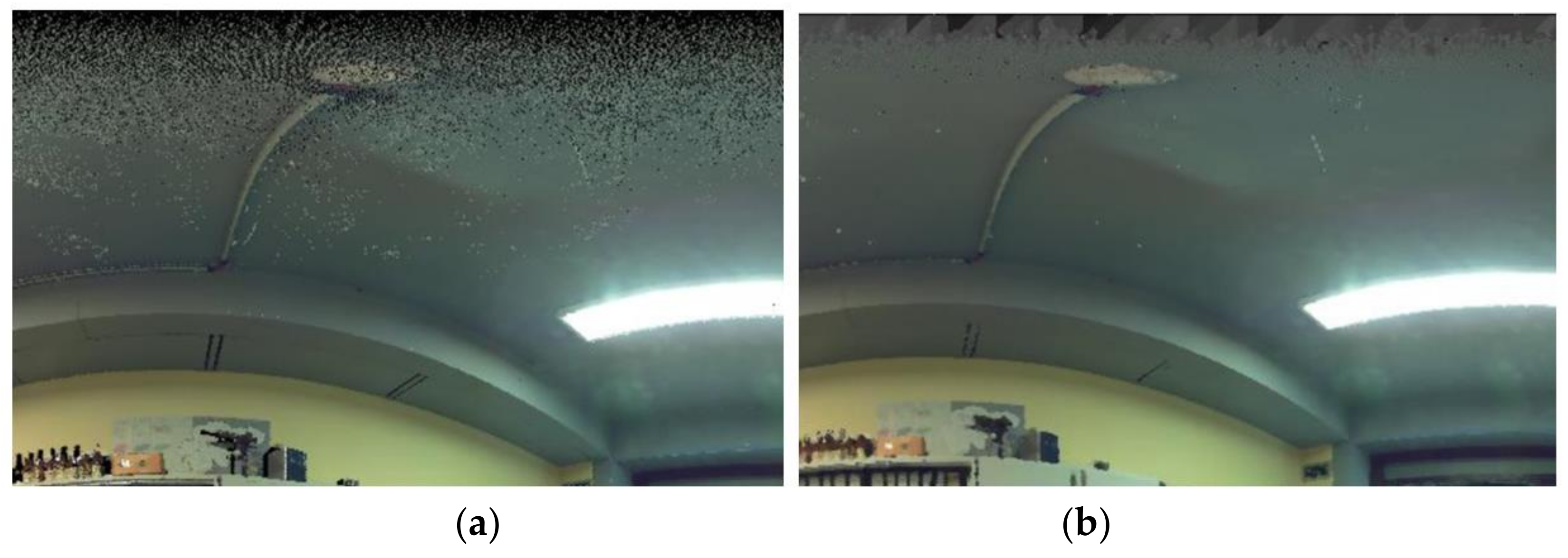
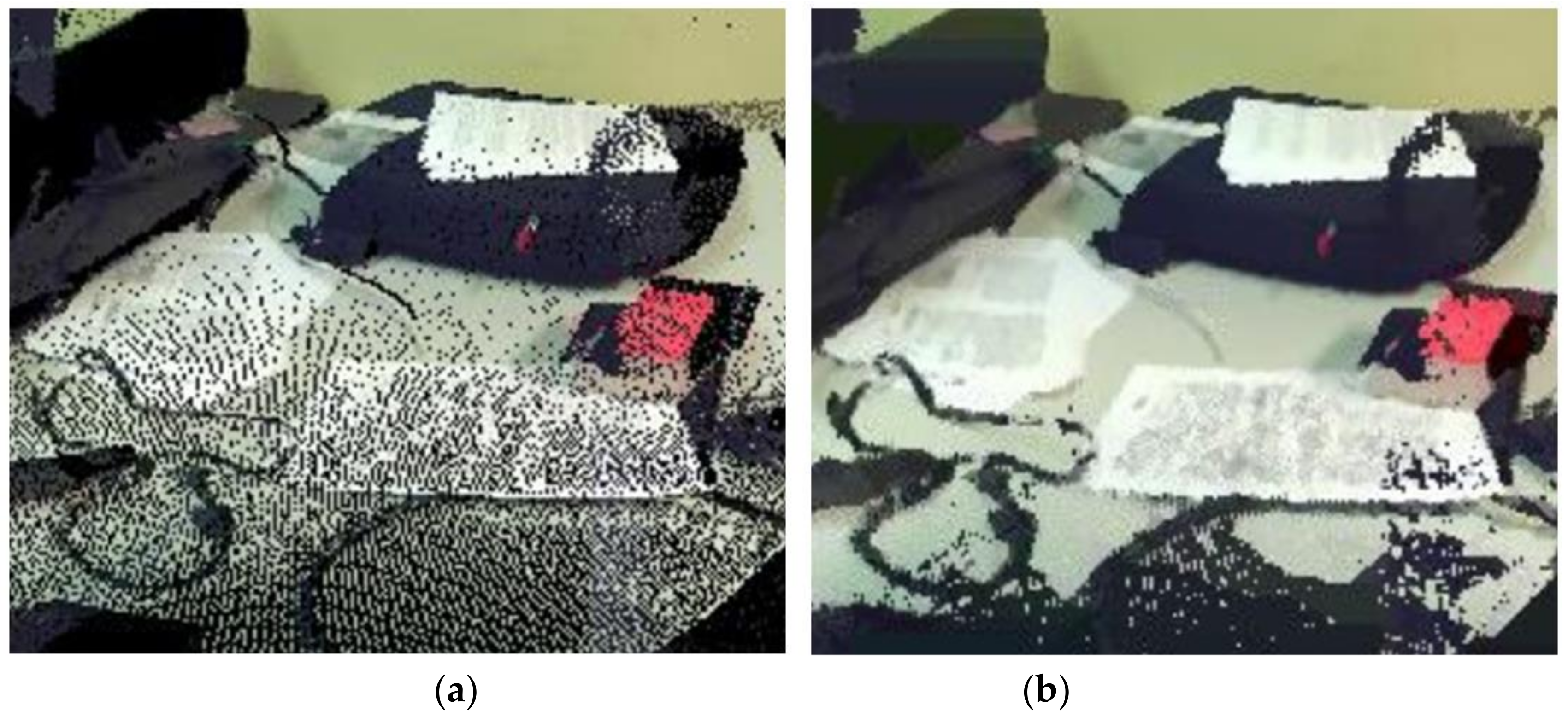
After reducing the artefacts and the small slots of the empty pixels, we still have some bigger voids that a simple fill filter can fill in. We have created a function that fills the whole filter window with the median value instead of changing only the central pixel’s value. A 5 × 5 median filter calculates this median value. However, in the case of the panoramic image in Figure 5, this function is only applied to pixels that have a colorimetric value lower than (30, 30, 30) so as not to alter the other nonempty pixels of the panoramic image and thus reduce the contrast even more. The value (30, 30, 30) is a subjective value considered after the application of several tests; further, it is only applicable for the panoramic image shown above, and thus, this value can change from one image to another. This filter was applied several times on the image until the desired result was obtained (Figure 6).

3.3. Cubemap Generation Using Cubic Projection

As a reminder, the curved projection called tiled (spherical and cylindrical), used to generate the previous panoramic image, generates deformations of the straight lines which become more curved as we move away from the central horizontal line of the image (all vertical straight lines are preserved unlike the horizontal ones). This represents a big disadvantage for the deep learning step, since the images that were used to train the neural model adopted in this research (Mask R-CNN) are normal images (not curved) generated with a rectilinear perspective projection, which is adopted by most digital cameras. Consequently, there is a high probability that the objects in the first panoramic image are not detected by the neural network, even in the case of a perfectly clear and homogeneous image. This is why the generation of a second panoramic image is required (the cubemap).
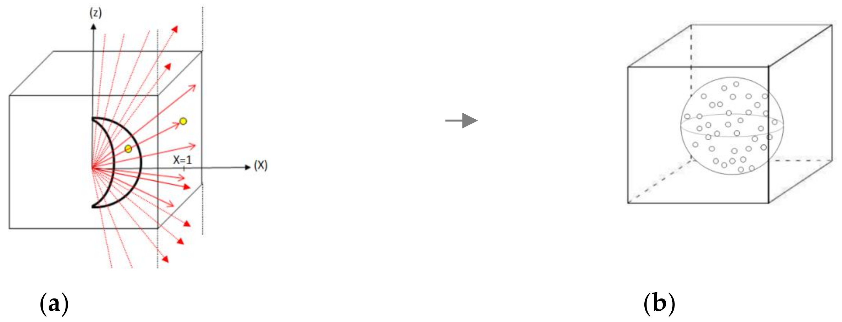
Unlike the tiled projections, the cubic projection preserves all the straight lines in reality, since it is a rather special projection that brings together six rectilinear projections (on the cube six facets) into a single projection. Thus, each facet of the cubemap looks like a typical image taken by a conventional digital camera. The cubemap presents a second significant advantage in this study, and we can easily dissect a cubemap either in several small images (facets) or in bands grouping together several facets. Subsequently, these faces and bands can be executed individually in the adopted neural network, and then, their results can be reintegrated into the original cubemap. Figure 7 below represents a sphere inside a cube. To generate the cubemap (panoramic image) from the point cloud projected onto the sphere using cubic projection, we apply the following mathematical steps:
Each point belonging to the sphere is centrally projected towards one of the six facets of the cube, so as to match each point to the correct facet. We first define four angle intervals according to the longitude of the sphere: 0 φ < π 2 , π 2 φ < π , π φ < 3 π 2 , 3 π 2 φ < 2 π . Point P′ has the following Cartesian coordinates: (x = r sin θ cos φ, y = r sin θ sin φ, z= r cos θ).
If we take, for example, the first region defined by the interval: 0 φ < π 2 , all the points that are part of this interval and which are projected centrally, would intersect with the plane of the first facet at x = 1 (figure below).
The projection of the point P′ (r sin θ cos φ, r sin θ sin φ, r cos θ) becomes (a sin θ cos φ, a sin θ sin φ, a cos θ), with ‘a’ being the radius of an imaginary sphere that shares the same centre and the same directions as our original sphere. We deduct the following relations:
a sin θ cos φ = x = 1 ,
Thus,
a = 1 sin   θ   cos   φ ,
Therefore, the coordinates of the projected point on the plane x = 1 become: P″ (1,   tan φ   , cot θ cos   φ ).
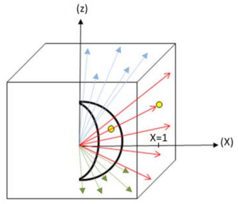
As we can notice in Figure 7, above, the points projected on the plane x = 1 do not all belong to the indicated 1st facet. Those which protrude at the top should rather be projected on the upper facet of the cube, and those which protrude at the bottom should be projected on the lower facet (Figure 8). Mathematically:
  • If 1 z = cot θ cos   φ 1 , the points are on the 1st facet, otherwise;
  • If z = cot θ cos   φ > 1 , these points are not considered and should rather be projected on the plane z = 1 (the top facet);
  • Otherwise, if z = cot θ cos   φ < 1 , these points should be projected on the plane z = −1.
The same process is applied to the three remaining regions. Thus, at the end, we obtain a point cloud in the form of a cube.
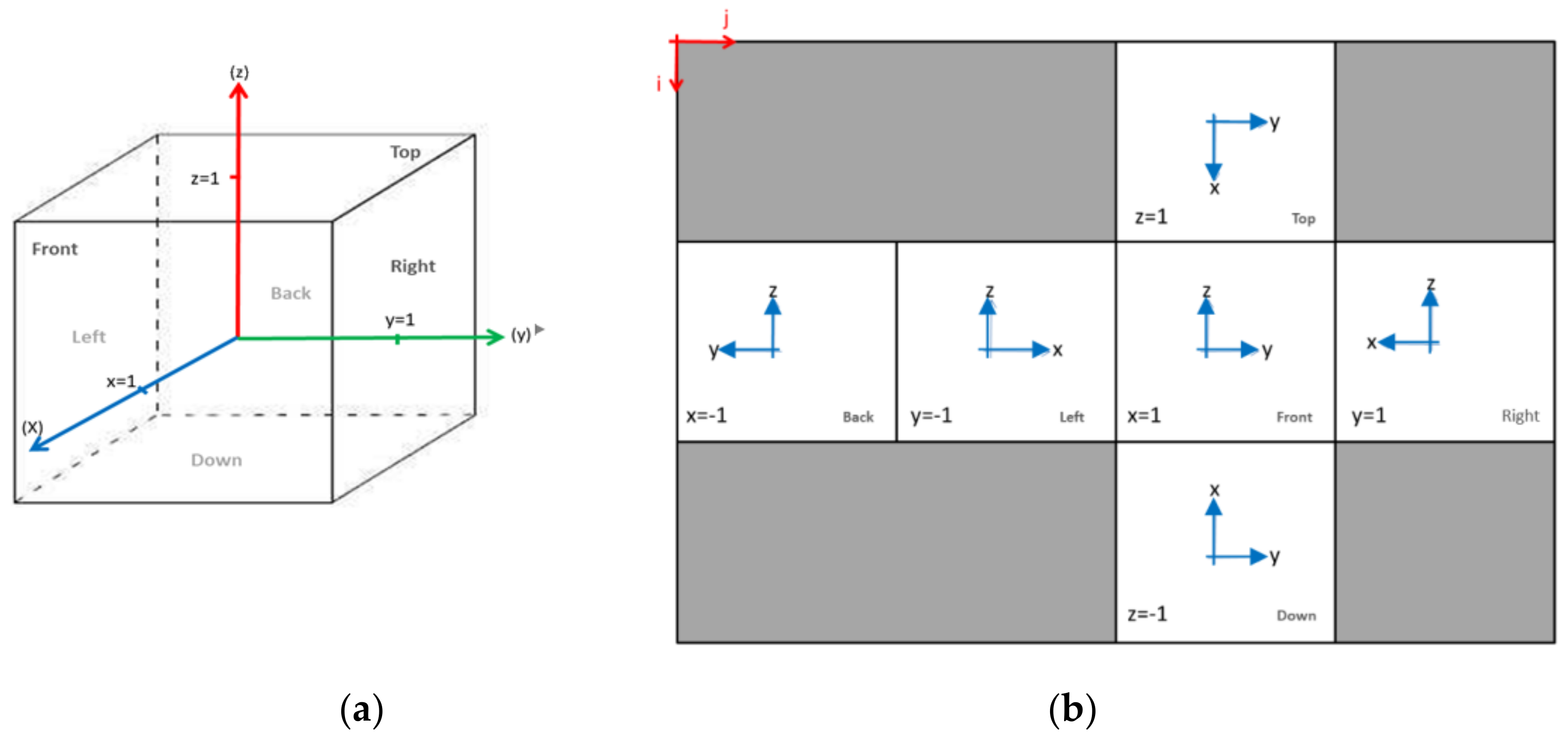
The next step consists of generating the cubemap which represents the flattened form of our cube, which means to find for each point of the point cloud in cube format its corresponding pixel in the cubemap. For this, we must first choose the configuration we want to have of the cubemap. Note that there are eleven nets of a cube. In our study, we opted for a cross net. The two figures below show the way of indexing the cubemap, respecting the way in which the cube was developed.
We start by choosing the desired width A of the cubemap (in pixels), such that the length of each edge is equal to A 4 and the resolution of the cubemap is (A, 3 × A 4 ). Each facet of the cubemap of Figure 9 contains in the canter: its old Cartesian coordinate system (respecting the way in which the cube was developed), which facilitates indexing thereafter, the name of the facet, and its projection plane. Table 1, below, summarises the image coordinates.
To benefit from the homogenisation that has already been applied to the first panoramic image (Figure 6), we create the cubemap based on it, by adding a small part to the mathematical model above. In fact, we apply the inverse of the equirectangular projection on the first panoramic image to have the points projected on the sphere again; after that, all that remains is to apply the formulae to pass from the sphere to the cubemap explained above.
The first algorithm generated in this study consists of directly applying the formulae explained previously by defining a projection function which takes the values θ and φ and returns the coordinates in a cube from −1 to 1 in each direction. Further, a second function takes the coordinates (x, y, z) of the points projected on the cube and transforms them into image coordinates of the output cubemap. This first algorithm’s logic consists of scanning the first panoramic image and for each pixel returning the position of the equivalent pixel in the cubemap. Figure 10, below, shows the result of the first approach of generating the cubemap.
The cubemap above shows a geometrically correct result. However, we notice the appearance of several black lines altering the visual aspect of our image. This comes down to the fact that our starting panoramic image has a resolution of (A/2, A), while the cubemap has a resolution of (3 × A/4, A), with ‘A’ being the width of the two panoramic images. This means that it is not a pixel by pixel projection since the dimension of the cubemap is greater in height than that of the first panoramic image, which generates the artifacts in the figure above. We solved this problem by taking a reverse approach but keeping the same projection logic; that is, instead of going through each pixel of the source (1st panoramic image) and finding the corresponding pixel in the target (cubemap), we scan the target image (cubemap), and for each pixel of the target (empty a priori), we find the closest corresponding source pixel in the 1st panoramic image. Finally, we assign the value of this pixel to the empty pixel of the cubemap. On the resulting cubemap from the reverse approach, (Figure 11) below, we notice the disappearance of artefacts related to the difference between the dimension of the first panoramic image and the cubemap.
Subsequently, the entire cubemap, facets and bands are separately integrated into the Mask R-CNN neural network to make more classification testing.

3.4. Instance Segmentation with Mask-RCNN

After ensuring the link between the two panoramic images pixels and the initial point cloud, the next step is to implement a neural network that ensures an automatic instance segmentation of these images using deep learning. To semantically segment the panoramic images, we chose to work with the Mask R-CNN model; this choice was mainly motivated by the following reasons:
  • The main reason is the fact that this model allows for a pixel level classification by outputting for each object of the input image a different colour mask, which is perfectly adapted to the logic of the developed program based on the back projection of the new pixel values after the semantic segmentation of the panoramic images. Models that only allow object detection, such as the R-CNN, fast R-CNN, or YOLO neural networks, are not suitable for this study since they only generate bounding boxes around the objects but not a dense classification at the pixel level;
  • This model is pretrained on the Microsoft COCO (Common Objects in Context) dataset and available under an open-source license on Github;
  • Published in 2017, it is one of the most popular models for instance segmentation today.
The Mask R-CNN model, developed by He et al. in 2017, is one of the most adopted and efficient models for instance segmentation tasks; it is a multistep approach that combines approaches used in the previous versions of the R-CNN series (Faster R-CNN and Fast R-CNN) and presents new improvements such as the RoIAlign method as well as the fully convolutional (FCN type network [9]) binary mask prediction branch, hence the name of the model. The model returns the bounding boxes, classes, and segmentation masks of the detected objects (Figure 12). Mask R-CNN adopts the same two-stage procedure, with an identical first stage (which is RPN [9]) [10]. The region proposal network (RPN) is in charge of “proposing” areas of the image that potentially contain an object, before the classification part which says whether each region (RoI) indeed contains an object worth detecting and which object it is. The RPN outputs a set of rectangular object proposals (four coordinates for each), each with the probability of containing an object [9]. Before the RPN, the input image passes in a backbone part for feature map extraction which is a ResNet-FPN ([46,47]) style deep neural network. It consists of a bottom-up pathway, a top-bottom pathway, and lateral connections (Figure 12). Using ResNet-FPN backbone for feature extraction with Mask R-CNN gives excellent gains in both accuracy and speed [10].
After the RPN phase, the resulting RoIs are warped to a fixed size before being introduced to the second stage of the mask R-CNN architecture (the classification/bounding box and mask branches). The improvement here is in the use of the method RoIAlign instead of the RoIPool used in the previous version: Faster R-CNN architecture. In fact, RoIPool [9] is a standard operation for extracting a small feature map (e.g., 7 × 7) from each RoI. That implies the quantisation of the strid in the max pooling operation, for example, for a RoI of 17 × 17, the required stride is 17/7 = 2.4, and since a stride of 2.4 is meaningless, RoIPool quantises this value by rounding it to 2, which introduces a loss of data and a misalignment between the RoI and the extracted features. While this may not impact classification, which is robust to small translations, it has a large negative effect on predicting pixel-accurate masks [10]. To avoid these problems, He et al. [10] developed the RoIAlign that implies no quantisation; therefore, in the case of the 17 × 17 RoI input region, we consider the 2.4 stride as it is, and for each cell in the RoI after devising it by the 2.4 stride, four sampling points are defined. RoIAlign computes the value of each sampling point by bilinear interpolation from the nearby grid points on the feature map, and finally, the chosen cell value is the max value between the four sampling points values, as for each of the RoI cells. No quantisation is performed on any coordinates involved in the RoI, its bins, or the sampling points [10] (Figure 13). Warped features (RoIs) are then fed into fully connected layers to make a classification using softmax, and boundary box prediction is further refined using the regression model. The same warped features are also fed into Mask classifier, which consists of a fully convolutional network (FCN [6]) to output a binary mask for each RoI.
The Mask R-CNN model used in this study was pretrained on the Microsoft COCO image dataset; its name literally implies that the images are everyday objects captured from everyday scenes. This adds context to the objects captured in the scenes. Moreover, it was created primarily to advance the state of the art in object recognition by placing the issue of object recognition in the context of the broader issue of scene understanding [48]. More concretely, the database is realised by gathering images of complex scenes containing common objects in their natural context; these images are labelled using instance segmentation. The particularity of this database is that it works better than previous ones for recognising objects on noncanonical images: containing objects in the background, partially occluded, in the middle of disorder, etc., reflecting the composition of natural daily scenes [48]. Figure 14 shows the 80 object categories considered by the COCO database with 330,000 images, containing 1.5 million labelled and segmented object instances.
To verify the correct implementation of the Mask R-CNN network in our program, we first tested the instance segmentation on random images. The result of instance segmentation on a random test image is shown in Figure 15.
The instance segmentation result is not suitable for our study for the two following reasons:
  • The resulting image contains in addition to object recognition masks: bounding boxes, prediction values, and object class names.
  • As an output, the code does not allow for the downloading of the segmented image but only its visualisation as a graph on the development environment used.
We have added a function that allows for the downloading of the images after their instance segmentation in several modes and with more functionalities to solve these two problems. This permits keeping only the segmentation masks with the input image in the background. Figure 16, below, shows the result of downloading the segmented image in mask mode only.
In addition to the download modes, the features that have been added are:
  • The choice of the prediction threshold.
  • The choice of the object classes to detect, allowing the user to filter the classes displayed in the network output.

3.5. Back Projection of Class Instances Predictions to the Point Cloud

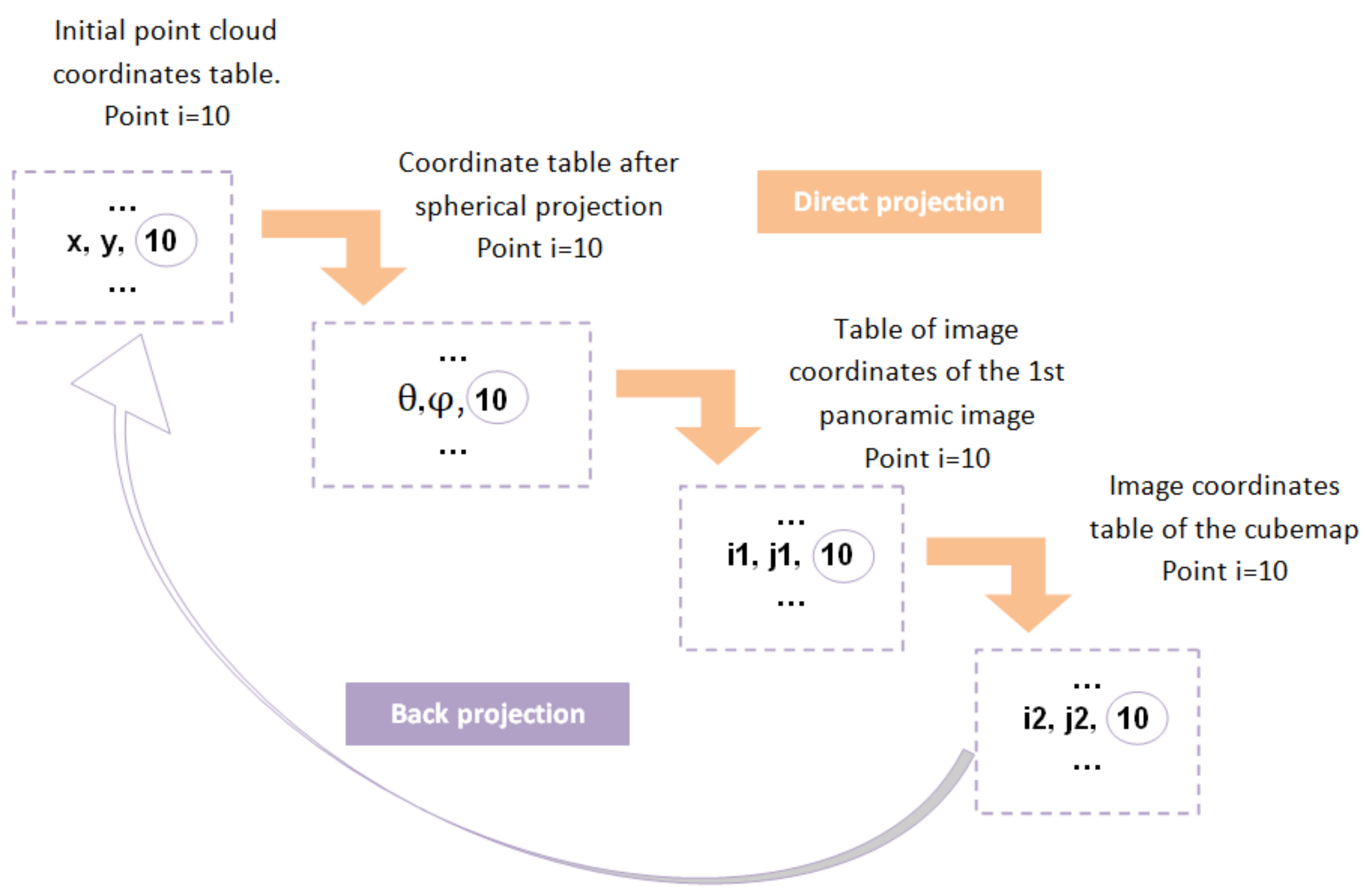
We recall that the objective of this study goes beyond the creation of the panoramic images and deals also with the semantic segmentation of the initial cloud of points. In fact, we have to ensure a link between each pixel of the panoramic image and its corresponding point in the cloud, so that we can use this link to segment our cloud after the segmentation of the panoramic image. A unique identifier ‘i’ expresses this link for each point, which has been introduced each time a new coordinate table is created in our program in order to ensure the preservation of the link with the points of the cloud throughout the whole development process. Figure 17, below, schematises an example of the link between the different coordinates at different phases allowing the back projection of the point (i = 10).
For instance, for the point with the identifier i = 10 above, each time we carry out a projection, we introduce the identifier i at the end of the new coordinates table to preserve the link with the initial point cloud. After the panoramic image semantic segmentation, we simply need to replace the colour values (R, G, B) of the initial point (point of the cloud with the identifier 10) by the new colour values (after instance segmentation) of pixel (i2, j2, 10) of the cubemap, based on the identifier i = 10. This exact process is applied to each of the panoramic image pixels.

4. Results

This section presents test results that have been carried out to validate our approach. Firstly, we present analyses and remarks related to each phase of the adopted process for the semantic augmentation of point clouds. Then, we present the test results on two different types of point clouds (clouds of interior environment and clouds of some specific objects).

4.1. Datasets

The Table 2 below summarises the point clouds used in this study and their properties. XYZ are the point coordinates; RGB are the point colour information; I the intensity; and D the depth.

4.2. The Optimal Resolution for the First Panoramic Image

When choosing the resolution of the 360° panoramic image, it is necessary to keep a certain balance on the image by adopting a resolution that preserves the richness of the initial point cloud and at the same time without generating an exaggerated number of empty pixels that could possibly influence the result of the automatic classification.
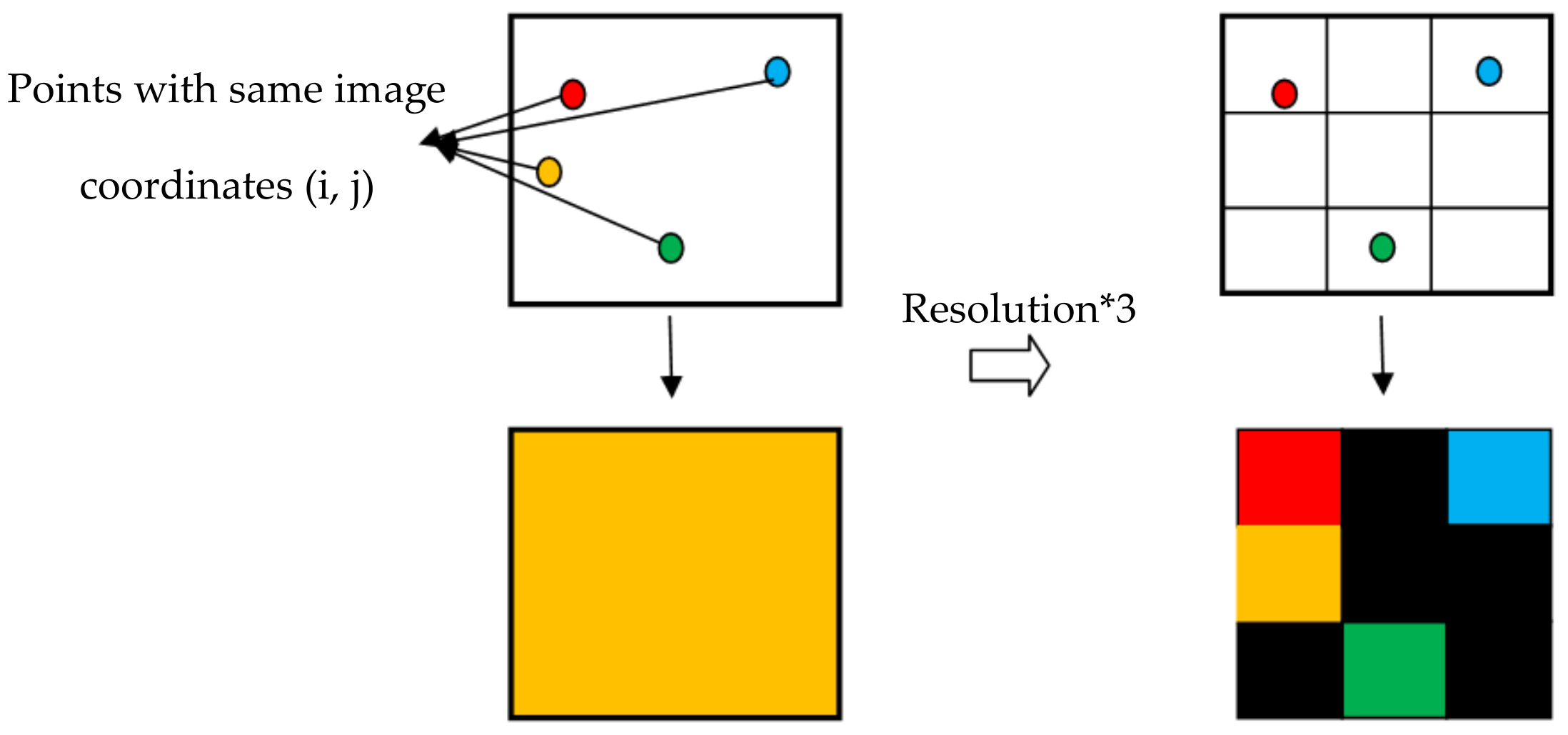
As an example, if we consider that the image coordinates of two different points (φ1, θ1) and (φ2, θ2) are (80.2, 21.4) and (80.1, 21), the function in the program would return, in reality, the integer values of (i, j) meaning the image coordinates (80, 21) for the first point and the same coordinates (80, 21) for the second point, and since a pixel can only take the colour information of a single point, the information of one of these points would not be considered, which implies a loss of data for some points of the cloud that have very close coordinates ‘φ’ and ‘θ’. To get around this problem, it is necessary to increase the resolution of the panoramic image, such that each pixel represents a very restricted angle field, thus increasing the chance that a single point of the cloud is in an angle field occupied by a pixel (Figure 18). This is illustrated by the figure below: the left part shows a single pixel of a low-resolution panoramic image, and only the orange pixel is considered, which induces a loss of the informative value of the other three pixels. On the other hand, we see in the right part that, with the increase in the resolution, each point occupies exactly one pixel; therefore, no data loss has occurred. However, the increase in resolution leads to the appearance of more empty pixels in the image (black pixels in Figure 18), but this is still treatable in comparison with the problem of loss of information value of the initial point cloud. The majority of these empty pixels are later eliminated in the image processing part. However, it is necessary to keep a certain balance by choosing a resolution that preserves the richness of the initial point cloud and at the same time does not generate an excessive number of empty pixels. In the case of the cloud (Figure 3), the resolution that has been chosen is 786 pixels in height and 786 × 2 in width (to keep the 2:1 ratio).
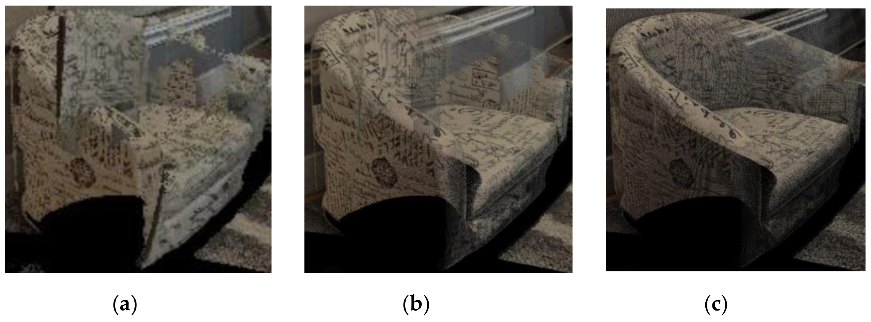
Figure 19, below, shows an example of the recuperation of certain parts of a chair with the increase in the resolution of the panoramic image.

4.3. Homogenisation of the 360° Panoramic Image

Disappearance of the artefacts related to the acquisition of the cloud (Figure 20).
Disappearance of empty pixels (recovery of the lamp), as well as the filling of the upper area that had an overabundance of empty pixels (Figure 21).
Appearance of blurring as the size of the median filter increases (Figure 22).
Recovery of writings on paper, as well as a loss of data in the regions where there is a dominance of empty pixels over useful pixels (Figure 23).
The more we increase the median filter size, the more the image becomes less noisy but, on the other hand, blurred. In addition, if the salt and pepper noise (empty pixels and artefacts) is more significant than half the median filter size, filtering is ineffective. Suppose the majority of the pixels in the window around a central pixel are noisy with empty pixels that have a very low grey level. In that case, the median filter would give this pixel a shallow grey level as well, and the pixel would be noisy ‘pepper’ in the filtered image. The same would be true for most pixels in the window that are noisy with artefact pixels that have a very high grey level. On the other hand, if in the window the number of noisy pixels ‘pepper’ and ‘salt’ are both less than half the size of the filter, then the median grey level of the window would be neither ‘pepper’ nor ‘salt’ but a non-noise value. This means that in the filtered image, the centre pixel would have a non-noise value.

4.4. Back Projection on the Point Cloud Analysis

4.4.1. Influence of the Projection Centre Position (Depth of the Cloud Points)

As explained in the previous part, in order to have a logical result on the panoramic image, the points projected on the image must represent the foreground view with respect to the projection centre (centre of the sphere). In another way, for an angle (φ, θ), only the point that has the smallest depth with respect to the projection centre is considered in the panoramic projection, and the other points are ignored in order to have a logical and understandable panoramic image. This obviously affects the result of the back projection of the predictions. The figure below shows the result of the back projection of a test panoramic image that has been fully coloured to detect the points of the cloud that have been taken into consideration in the projection process. We notice that the areas that are close to the projection centre (red point) contain more segmented points compared to the areas that are far from the centre, for example: areas (1) and (2) in Figure 24 below (points ignored during the projection of the panoramic image due to the condition on the depth regarding the points to be considered).

4.4.2. Influence of Panoramic Image Resolution on Cloud Segmentation

One of the major difficulties encountered in this study is how to efficiently merge 2D and 3D domain data. This is quite difficult for the following reasons: there is generally no one-to-one mapping between 2D and 3D data; the 2D and 3D neighbourhood definitions are different; and further, neighbouring pixels in an image are defined by a very regular grid, while 3D points are defined at nonuniform continuous locations.
To overcome these problems, it is necessary to choose the resolution of the panoramic image that allows segmenting the maximum number of points on the cloud while paying attention to the number of empty generated pixels, which could negatively influence the result of automatic detection by the neural network used.
In Figure 25, we notice that the resolution of the panoramic image has a big influence on the segmentation rate of the cloud after the back projection. This comes back to the influence of the resolution on the preservation of the informational richness of the cloud points on the projected panoramic image (Figure 18). In fact, if the resolution is high, we would have a larger number of segmented pixels on the panoramic image (these pixels are obviously related to the points of the initial cloud), hence the increase in the number of segmented points on the cloud after the back projection. The image on the left represents the visualisation on Potree [44] of a point cloud derived from the segmentation of two objects on a panoramic image of (786, 1572) resolution, while the image on the right represents the same cloud derived from the segmentation of a panoramic image of (2000, 4000) resolution.

4.4.3. Influence of the Scattered Structure of the Point Cloud

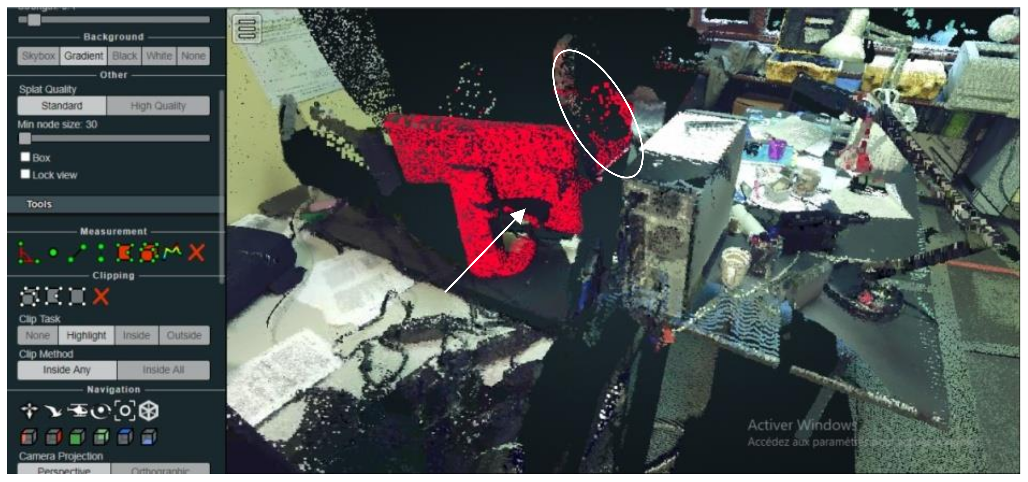
While neighbouring pixels in a panoramic image are defined by a regular grid, 3D points are defined at irregular and nonuniform locations. In fact, the scattered nature of the point cloud negatively influences the segmentation quality; more precisely, it influences the accuracy of the segmented objects on the cloud, even if the depth condition is respected for points that are in the same angle line (φ, θ). The problem here is not the depth, but the holes between the points of the objects in the cloud. For example, in the figure below, we notice that the object ‘computer’ contains in addition to the normal holes between the scattered points, a large empty area (shown by an arrow); therefore, during the spherical projection with respect to the centre of projection (point in red encircled in Figure 26), the points behind the computer with respect to this empty area appear inside the computer in the panoramic image. Therefore, after the segmentation of the computer on the panoramic image, these points (which do not belong to the computer but are projected in the panoramic image inside the computer) are also considered as points belonging to this object (Figure 26). That is why in the case of objects with a lot of empty areas and low density, we always have badly segmented points left behind, even if the depth condition is applied, except in the case of objects that do not overlap with other objects on the cloud.

4.5. Analysis of Instance Segmentation by Mask R-CNN

In this section, we present the results obtained by the segmentation of different point clouds. The two scenes ‘female statue’ and ‘office scene’ were acquired by the ULiège geomatics unit team. The rest of the clouds were downloaded from the Web database “Indoor Lidar-RGBD Scan Dataset” in order to have a fairly significant sample of different point clouds. This dataset contains five different complete indoor environments that were collected using a “FARO Focus 3D X330 HDR” scanner [49]. Each scene was scanned from several locations, and then the scans were merged using an unspecified alignment software. The clouds are in “PLY” format.
We chose to use this database since it contains very dense clouds, representing indoor environments and containing objects taken into account by the COCO image dataset with which the Mask R-CNN was trained.
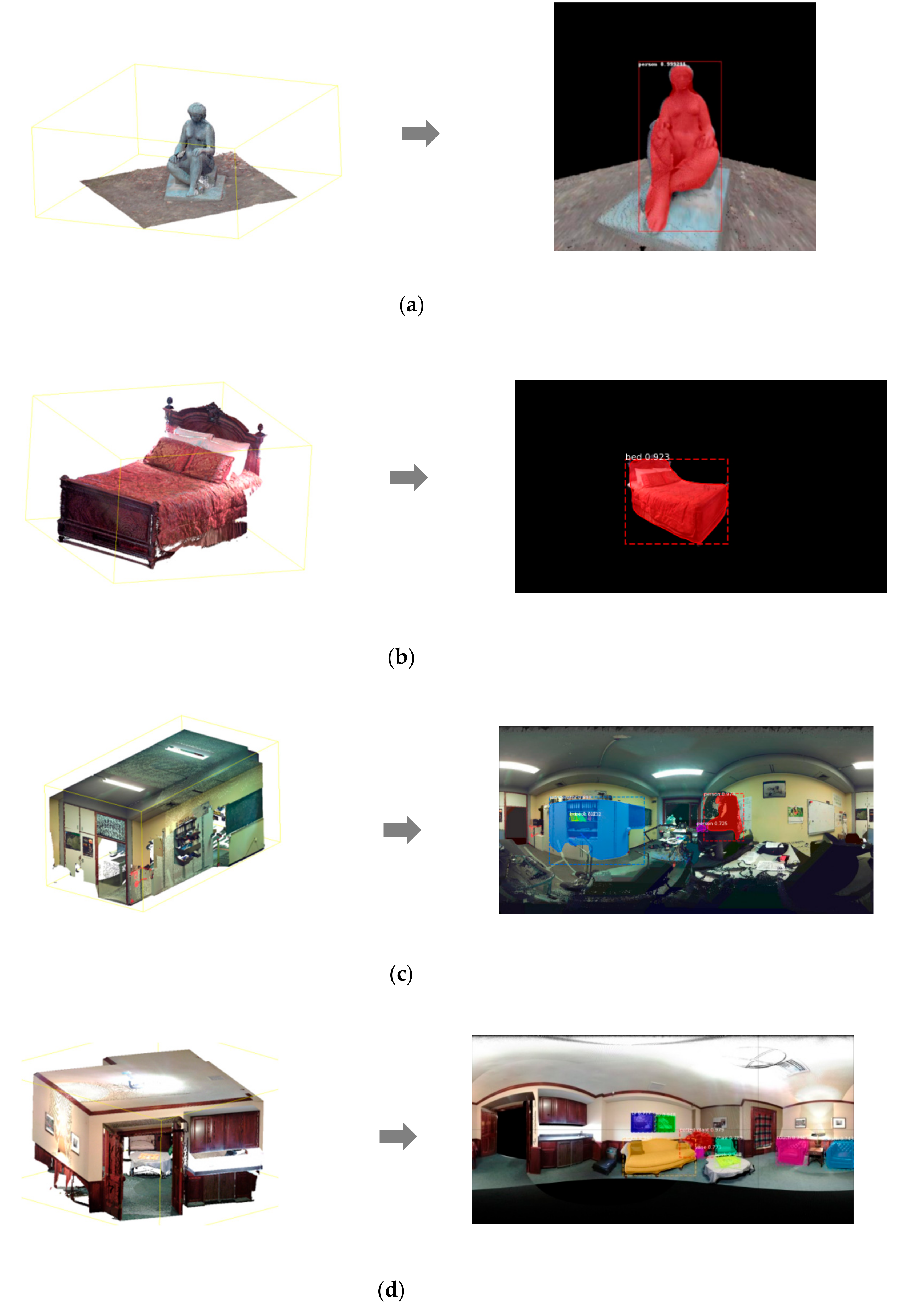
We notice that the developed approach works very well for clouds containing distinct objects (Figure 27: (1) and (2)). The first detection gives a prediction value of 0.999 for the object class ‘person’ and a value of 0.923 for the ‘bed’ class. Note that we did not expect to have the class ‘statue’ for the first point cloud, since the network is not trained to differentiate between a statue and a person.
On the second point cloud, we did not need to generate a cubemap since the shape of the bed has not been greatly altered by the spherical and cylindrical projections. However, the instance segmentation in the second case was performed on a single facet of the cubemap. Subsequently, we reintegrated the segmented facet into the cubemap in order to be able to carry out the backward projection towards the initial point cloud.
The third point cloud presents a 3D indoor (office) environment. In fact, this cloud is very complex to segment semantically for the following reasons: low-density cloud containing several large empty areas; very crowded scene with overlapping objects in several places; and incomplete objects (example: computer).
We recall that the only objects that can be detected on these point clouds are those taken into account by the COCO library (Figure 14). In this third cloud (Figure 27), the only objects that can be detected are: book, table, computer, ball, and person.
We notice that only the objects ‘person’ (in purple) and ‘book’ (in yellow and green) were correctly detected and segmented. This is why we proceeded with the second projection (cubic projection) in order to eliminate the distortion effect related to tiled projections (spherical and cylindrical), thus increasing the chances of correct predictions. The cubemap generated after the cubic projection was subdivided into six distinct facets, and then each facet was introduced individually into the Mask R-CNN network. The facet presented in the Figure 28 gave the best result compared to the other facets of the cubemap.
We notice that there is an improvement in detection on the facet above compared to the first panoramic image in tiled projection. More ‘book’ objects as well as the ‘ball’ object (in green) have been detected. The COCO library does not take into account the ‘closet’ object, which is why it was detected as a refrigerator (in orange and red).
The last example also represents an indoor environment (Figure 27), but it is a much denser and clearer cloud, containing fewer overlapping objects. In fact, most of the objects in the COCO database have been detected and segmented, notably the objects ‘armchair’, ‘vase’, ‘plant’, and ‘chair’, with prediction values between 0.74 and 0.98.
Results were validated by using the quality measures, such as Precision, Recall, and F1-score. The extracted objects are classified into the following three classes: True Positives is the surface in the extracted result which is correctly classified; False Positive is the surface in the extracted result which is incorrectly classified; and False Negative is the region which is present in the reference data as a specific object but is absent in the extracted result. The classes defined before are used to calculate the well-known quality measures such as Precision, Recall, and F1 score as shown below. Figure 29 illustrates the adopted method to calculate the quality measures.
Only the first, second, and forth point clouds (Figure 27) have been taken into consideration for quality measures, as the third point cloud was too complicated for the algorithm to extract good results. Since it is an instance segmentation method, we proceeded to calculate the quality measures for each separate object in each point cloud. Lastly, we calculated the average, minimum, and maximum for the Precision, Recall, and F1-score values (Table 3).

4.6. Comparison with the Approach Developed by Tabkha in 2019

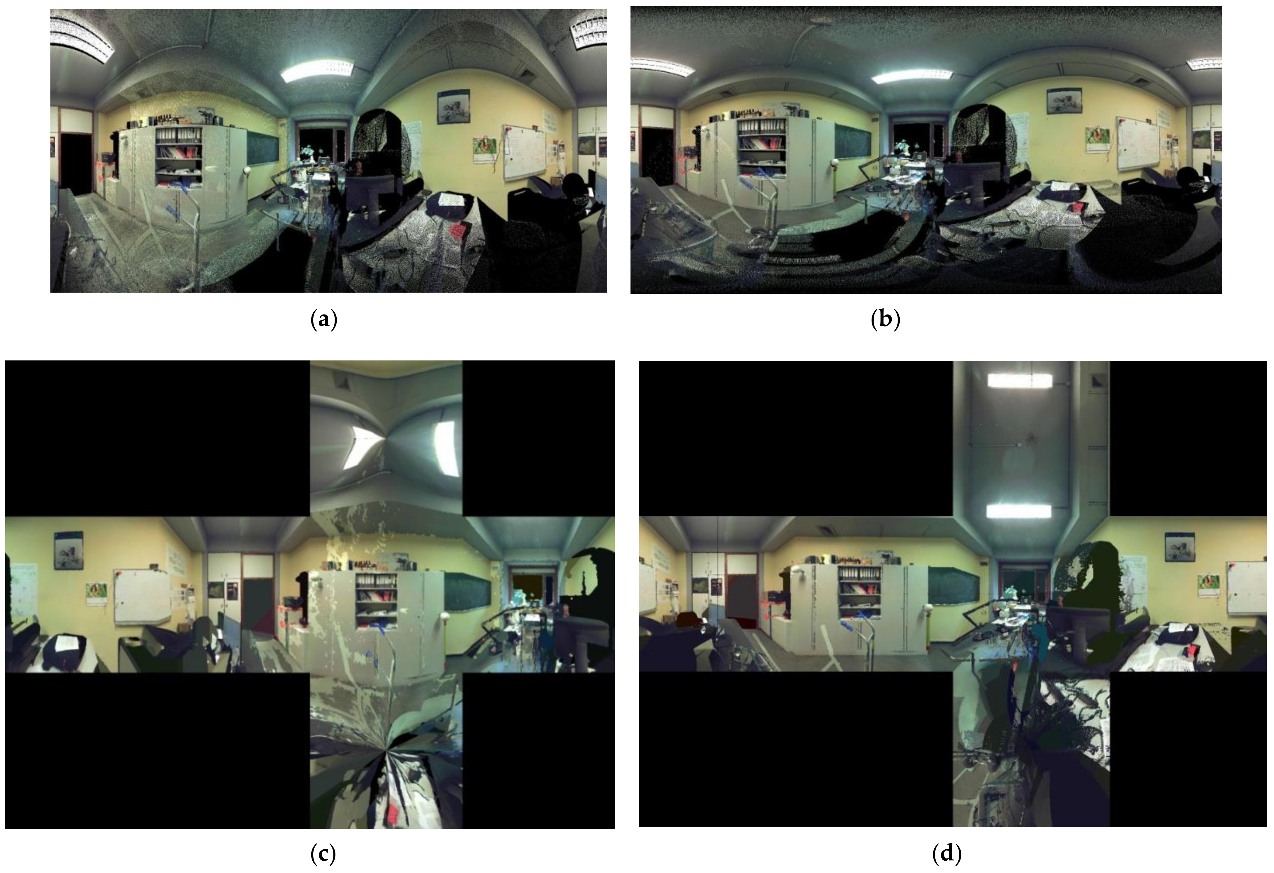
In the first row (Figure 30), we notice that thanks to the adoption of the spherical projection followed by the equirectangular cylindrical projection in the current study, a considerable part of the point cloud was recovered, notably the ceiling and the floor. Thus, we preserve the richness of the initial point cloud in its entirety. In the second row, we notice that the upper and lower facet were deformed due to the lack of data at floor and ceiling level in the panoramic image generated by Tabkha (2019) [20]. On the other hand, the cubemap generated by our approach gives a geometrically correct image.
For matters of comparison, we performed classification tests using the same ‘Imagga’ API used by Tabkha in 2019 [20]. The first table below (Table 4) shows the classification result of the panoramic image generated by Tabkha’s approach. The second table below (Table 5) shows the classification result by our approach using the cubemap band generated from the 360° panoramic image of the present approach (using spherical and cylindrical equirectangular projections). We notice a considerable improvement in classes and prediction values.

5. Discussion

Extracting semantics from point clouds has led to several approaches based on DL being investigated. Many state-of-the-art methods have been developed that process point cloud directly despite the challenging aspect of its unstructured and irregular format [4,32,34,35,36,37,38]. Other approaches convert the point cloud data into a structured form [50,51,52,53], and our research goes in the same direction. We have developed an approach based on an indirect process. Rather than having a point cloud in raw 3D format as the input of the neural network, we applied a transformation on the cloud to extract a 2D raster representation in the form of panoramic images. Then, these images were introduced as inputs of the adopted neural network.
This research’s strengths consist of, first, avoiding the challenges that come with working on DL in a 3D environment such as the irregular and unstructured format of point clouds. Secondly, we chose to use a pretrained neural network for the classification, which is one of the most important reasons to work in a 2D environment, as many labelled datasets with a large number of classes are available online. Third, according to the tests performed in the previous parts, our approach gives good results for instance segmentation. Most of the objects taken into account by the COCO dataset used to train the Mask R-CNN network have been well classified and segmented. For further investigation, it is very recommended to train Mask R-CNN on other available datasets and see how the algorithm responds to the new tests, thus supporting the validation of the segmentation and classification step. We also believe that the algorithm can give good detection results for larger-scale point clouds, but they must remain simple in terms of the number of objects and their superimpositions in the cloud.
Regarding the time and power constraints, the projection part of the algorithm is largely dependent on the size of the initial point cloud: the larger the size of the point cloud and the resolution chosen for the panoramic images, the more time it would require, which can easily go from a few minutes for small point clouds (first, second, and third points clouds in Figure 27, for instance) to half an hour or even more for very large ones (fourth point cloud in Figure 27). For the segmentation/classification step and since we use a powerful pretrained neural network, the detection usually takes a few seconds, even while using the computing power of Google Colaboratory, which allows one to run the code in the cloud and enables us with a free access to GPU (Nvidia K80/T4).
The objective of improving the predictive system used by Tabkha (2019) [20] was also largely achieved by completely changing the panoramic projection logic and adopting a robust neural network for instance segmentation. In fact, the solution adopted in this study allows three main improvements compared to Tabkha’s solution:
  • The projection of all the points of the cloud on the panoramic image by adopting a spherical projection followed by another cylindrical one, which cannot be achieved if only by a cylindrical projection.
  • The addition of the cubic projection first allowed to get rid of the alterations caused by tiled projections (spherical and cylindrical projections). Secondly, the cubemap has allowed more input image options that we can use as a basis for instance segmentation (cubemap itself, strips, and individual facets).
More generally, the most significant advantage of our approach is that it opens the door to all the research carried out over the last decade on 2D images to 3D point clouds. This is exactly what has been proven using the Mask R-CNN neural network initially designed for the instance segmentation of 2D data only (images/videos).
Although the process developed has given good results, the approach does not escape certain imperfections:
  • The influence of the projection centre position choice on the results of the instance segmentation.
  • The need to multiply the projections from several positions to allow the segmentation of a point cloud composed of many “subspaces”. A single projection from a single virtual camera position is not enough to segment the entire cloud, given the depth condition (only points in the foreground view of the camera can be segmented).
  • The difficulty of choosing a good panoramic image resolution that allows one to have a balance between preserving the richness of the initial point cloud without generating a great number of empty pixels. Therefore, it is necessary to carry out several projection tests to find the optimal resolution.
  • The scattered structure of the cloud’s points decreases the accuracy of object segmentation (example of the segmentation of the ‘computer’ object in the previous chapter).

6. Conclusions

We propose a complete workflow for the instance segmentation of 3D point clouds by using a deep learning architecture trained on radically different data modalities and contexts. Our workflow starts by projecting 3D point clouds into optimised 2D images, using different types of panoramic projections. These are then used as input of the Mask R-CNN neural network pretrained on the Microsoft COCO dataset of 2D images. Finally, we project the predictions of the semantically segmented images back to the initial point clouds, based on the retained links between panoramic image pixels and 3D points. Our approach tested on different point clouds demonstrates promising research directions by leveraging robust deep learning models to identify objects in 3D scenes. On one hand, our current application allows one to: (1) detect and segment objects composing a scene with an accuracy above 70%, (2) attach robust scene classification for point cloud contextualisation, and (3) extend to domain-specific instance segmentation with a potentially unlimited number of detected classes. On the other hand, the approach developed has demonstrated a considerable improvement over that of Tabkha’s (2019) in terms of preserving the information richness of the initial point cloud, since it is first projected on a sphere and not a cylinder that causes the elimination of the upper and lower parts of the cloud, and also, improvements in detection results have been noticed that come down to the fact that with our approach, more parts of the point cloud scene are preserved which help a better context detection by the API Imagga neural network.

Author Contributions

Conceptualization, G.K. and F.P.; methodology, G.K.; software, G.K.; validation, G.K., F.P. and R.H.; formal analysis, G.K.; investigation, G.K. and F.P.; resources, G.K. and F.P.; data curation, G.K. and F.P.; writing—original draft preparation, G.K.; writing—review and editing, G.K., F.P. and R.H.; visualisation, G.K.; supervision, F.P. and R.H.; project administration, F.P.; funding acquisition, F.P. All authors have read and agreed to the published version of the manuscript.

Funding

This research received no external funding.

Institutional Review Board Statement

Not applicable.

Informed Consent Statement

Not applicable.

Conflicts of Interest

The authors declare no conflict of interest.

References

  1. Poux, F. The Future of 3D Point Clouds: A New Perspective, Towards Data Science. Available online: https://towardsdatascience.com/the-future-of-3d-point-clouds-a-new-perspective-125b35b558b9 (accessed on 29 May 2021).
  2. Poux, F.; Billen, R. Voxel-based 3D Point Cloud Semantic Segmentation: Unsupervised geometric and relationship featuring vs deep learning methods. ISPRS Int. J. Geo-Inf. 2019, 8, 213. [Google Scholar] [CrossRef] [Green Version]
  3. He, Y.; Yu, H.; Liu, X.; Yang, Z.; Sun, W.; Wang, Y.; Fu, Q.; Zou, Y.; Mian, A. Deep Learning based 3D Segmentation: A Survey; Deep Learning based 3D Segmentation: A Survey. arXiv 2021, arXiv:2103.05423. [Google Scholar]
  4. Landrieu, L.; Simonovsky, M. Large-scale Point Cloud Semantic Segmentation with SuperpointGraphs. arXiv 2017, arXiv:1711.09869. [Google Scholar]
  5. Topiwala, A. Spherical Projection for Point Clouds, Towards Data Science. Available online: https://towardsdatascience.com/spherical-projection-for-point-clouds-56a2fc258e6c (accessed on 31 May 2021).
  6. Long, J.; Shelhamer, E.; Darrell, T. Fully convolutional networks for semantic segmentation. arXiv 2015, arXiv:1411.4038. [Google Scholar]
  7. Girshick, R.; Donahue, J.; Darrell, T.; Malik, J. Rich feature hierarchies for accurate object detection and semantic segmentation. arXiv 2013, arXiv:1311.2524. [Google Scholar]
  8. Girshick, R. Fast R-CNN. arXiv 2015, arXiv:1504.08083. [Google Scholar]
  9. Ren, S.; He, K.; Girshick, R.; Sun, J. Faster R-CNN: Towards Real-Time Object Detection with Region Proposal Networks. arXiv 2016, arXiv:1506.01497. [Google Scholar] [CrossRef] [PubMed] [Green Version]
  10. He, K.; Gkioxari, G.; Dollár, P.; Girshick, R. Mask R-CNN. arXiv 2017, arXiv:1703.06870. [Google Scholar]
  11. Redmon, J.; Divvala, S.; Girshick, R.; Farhadi, A. You Only Look Once: Unified, Real-Time Object Detection. arXiv 2015, arXiv:1506.02640. [Google Scholar]
  12. Blaschke, T. Object based image analysis for remote sensing. ISPRS J. Photogramm. Remote Sens. 2010, 65, 2–16. [Google Scholar] [CrossRef] [Green Version]
  13. Guirado, E.; Tabik, S.; Alcaraz-Segura, D.; Cabello, J.; Herrera, F. Deep-learning Versus OBIA for scattered shrub detection with Google Earth imagery: Ziziphus lotus as case study. Remote Sens. 2017, 9, 1220. [Google Scholar] [CrossRef] [Green Version]
  14. Li, X.; Shao, G. Object-based land-cover mapping with high resolution aerial photography at a county scale in midwestern USA. Remote Sens. 2014, 6, 11372–11390. [Google Scholar] [CrossRef] [Green Version]
  15. Pierce, K. Accuracy optimization for high resolution object-based change detection: An example mapping regional urbanization with 1-m aerial imagery. Remote Sens. 2015, 7, 12654–12679. [Google Scholar] [CrossRef] [Green Version]
  16. Tiede, D.; Krafft, P.; Füreder, P.; Lang, S. Stratified template matching to support refugee camp analysis in OBIA workflows. Remote Sens. 2017, 9, 326. [Google Scholar] [CrossRef] [Green Version]
  17. Laliberte, A.S.; Rango, A.; Havstad, K.M.; Paris, J.F.; Beck, R.F.; McNeely, R.; Gonzalez, A.L. Object-oriented image analysis for mapping shrub encroachment from 1937 to 2003 in southern New Mexico. Remote Sens. Environ. 2004, 93, 198–210. [Google Scholar] [CrossRef]
  18. Hellesen, T.; Matikainen, L. An object-based approach for mapping shrub and tree cover on grassland habitats by use of LiDAR and CIR orthoimages. Remote Sens. 2013, 5, 558–583. [Google Scholar] [CrossRef] [Green Version]
  19. Stow, D.; Hamada, Y.; Coulter, L.; Anguelova, Z. Monitoring shrubland habitat changes through object-based change identification with airborne multispectral imagery. Remote Sens. Environ. 2008, 112, 1051–1061. [Google Scholar] [CrossRef]
  20. Tabkha, A.; Hajji, R.; Billen, R.; Poux, F. Semantic enrichment of point cloud by automatic extraction and enhancement of 360° panoramas. Int. Arch. Photogramm. Remote Sens. Spatial Inf. Sci. 2019, 42, 355–362. [Google Scholar] [CrossRef] [Green Version]
  21. Frich, A. What Is a Panoramic Photography? 2019. Available online: https://www.panoramic-photo-guide.com/panoramic-photography.html (accessed on 31 May 2021).
  22. Labracherie, R.; Numérique, F.; Thomas, M. La Photographie Panoramique #1: Les Prérequis—Les Numériques. Available online: https://www.lesnumeriques.com/photo/la-photographie-panoramique-1-les-prerequis-pu100641.html (accessed on 31 May 2021).
  23. La Perspective Conique. Available online: http://dam.archi.free.fr/1A1S/Descriptive/Cours5.pdf (accessed on 31 May 2021).
  24. Britannica. Mercator Projection. Definition, Uses, & Limitations. Available online: https://www.britannica.com/science/Mercator-projection (accessed on 31 May 2021).
  25. Mercator Projection—An Overview, ScienceDirect Topics. Available online: https://www.sciencedirect.com/topics/earth-and-planetary-sciences/mercator-projection (accessed on 12 July 2021).
  26. Houshiar, H.; Elseberg, J.; Borrmann, D.; Nüchter, A. A study of projections for key point based registration of panoramic terrestrial 3D laser scan. Geo-Spat. Inf. Sci. 2015, 18, 11–31. [Google Scholar] [CrossRef]
  27. Equirectangular Projection—Wikipedia. Available online: https://en.wikipedia.org/wiki/Equirectangular_projection (accessed on 31 May 2021).
  28. Sharpless, T.K.; Postle, B.; German, D.M. Pannini: A new projection for rendering wide angle perspective images. In Computational Aesthetics in Graphics, Visualization, and Imaging; Jepp, P., Deussen, O., Eds.; The Eurographics Association: Geneva, Switzerland, 2010. [Google Scholar]
  29. Brown, M. Content-Aware Projection for Tiny Planets; Short Papers; Eurographics: Geneva, Switzerland, 2015. [Google Scholar]
  30. Mirror Ball, Angular Map and Spherical. Available online: https://horo.ch/docs/mine/pdf/Mb-Am-Sph.pdf (accessed on 31 May 2021).
  31. Bello, S.A.; Yu, S.; Wang, C. Review: Deep learning on 3D point clouds. arXiv 2020, arXiv:2001.06280. [Google Scholar] [CrossRef]
  32. Qi, C.R.; Su, H.; Mo, K.; Guibas, L.J. PointNet: Deep Learning on Point Sets for 3D Classification and Segmentation. In Proceedings of the 30th IEEE Conference on Computer Vision and Pattern Recognition (CVPR 2017), Honolulu, HI, USA, 21–26 July 2017; pp. 77–85. [Google Scholar]
  33. Oster, M.; Douglas, R.; Liu, S.C. Computation with spikes in a winner-take-all network. Neural Comput. 2009, 21, 2437–2465. [Google Scholar] [CrossRef] [Green Version]
  34. Qi, C.R.; Yi, L.; Su, H.; Guibas, L.J. PointNet++: Deep hierarchical feature learning on point sets in a metric space. Adv. Neural Inf. Process. Syst. 2017, 2017, 5100–5109. [Google Scholar]
  35. Hu, Q.; Yang, B.; Xie, L.; Rosa, S.; Guo, Y.; Wang, Z.; Trigoni, N.; Markham, A. RandLA-Net: Efficient semantic segmentation of large-scale point clouds. In Proceedings of the IEEE Computer Society Conference on Computer Vision and Pattern Recognition, Longbeach, CA, USA, 16–20 June 2019; pp. 11105–11114. [Google Scholar]
  36. Li, Y.; Bu, R.; Sun, M.; Wu, W.; Di, X.; Chen, B. PointCNN: Convolution On X-Transformed Points. arXiv 2018, arXiv:1801.07791. [Google Scholar]
  37. Thomas, H.; Qi, C.R.; Deschaud, J.-E.; Marcotegui, B.; Goulette, F.; Guibas, L.J. KPConv: Flexible and Deformable Convolution for Point Clouds. In Proceedings of the IEEE International Conference on Computer Vision, Seoul, Korea, 27–28 October 2019; pp. 6410–6419. [Google Scholar]
  38. Wang, Y.; Sun, Y.; Liu, Z.; Sarma, S.E.; Bronstein, M.M.; Solomon, J.M. Dynamic Graph CNN for Learning on Point Clouds. ACM Trans. Graph. 2018, 38, 13. [Google Scholar] [CrossRef] [Green Version]
  39. Gu, J.; Wang, Z.; Kuen, J.; Ma, L.; Shahroudy, A.; Shuai, B.; Liu, T.; Wang, X.; Wang, L.; Wang, G.; et al. Recent Advances in Convolutional Neural Networks. arXiv 2015, arXiv:1512.07108. [Google Scholar] [CrossRef] [Green Version]
  40. Basha, S.H.S.; Dubey, S.R.; Pulabaigari, V.; Mukherjee, S. Impact of fully connected layers on performance of convolutional neural networks for image classification. Neurocomputing 2019, 378, 112–119. [Google Scholar] [CrossRef] [Green Version]
  41. Coursera. Convolutional Neural Networks. Available online: https://www.coursera.org/learn/convolutional-neural-networks (accessed on 31 May 2021).
  42. He, K.; Zhang, X.; Ren, S.; Sun, J. Spatial pyramid pooling in deep convolutional networks for visual recognition. Lect. Notes Comput. Sci. 2014, 8691, 346–361. [Google Scholar] [CrossRef] [Green Version]
  43. Liu, W.; Anguelov, D.; Erhan, D.; Szegedy, C.; Reed, S.; Fu, C.-Y.; Berg, A.C. SSD: Single shot multibox detector. Lect. Notes Comput. Sci. 2015, 9905, 21–37. [Google Scholar] [CrossRef] [Green Version]
  44. Schütz, M.; Ohrhallinger, S.; Wimmer, M. Fast out-of-core octree generation for massive point clouds. Comput. Graph. Forum 2020, 39, 155–167. [Google Scholar] [CrossRef]
  45. Bergounioux, M. Quelques Méthodes de Filtrage en Traitement d’Image. ffhal-00512280v2. 2011. Available online: https://hal.archives-ouvertes.fr/file/index/docid/569384/filename/CoursFiltrage.pdf (accessed on 20 July 2021).
  46. Lin, T.-Y.; Dollár, P.; Girshick, R.; He, K.; Hariharan, B.; Belongie, S. Feature Pyramid Networks for Object Detection. arXiv 2016, arXiv:1612.03144. [Google Scholar]
  47. He, K.; Zhang, X.; Ren, S.; Sun, J. Deep Residual Learning for Image Recognition. arXiv 2015, arXiv:1512.03385. [Google Scholar]
  48. Lin, T.Y.; Maire, M.; Belongie, S.; Hays, J.; Perona, P.; Ramanan, D.; Dollár, P.; Zitnick, C.L. Microsoft COCO: Common objects in context. In Proceedings of the Lecture Notes in Computer Science (Including Subseries Lecture Notes in Artificial Intelligence and Lecture Notes in Bioinformatics); Springer: Cham, Switzerland, 2014; Volume 8693 LNCS, pp. 740–755. [Google Scholar]
  49. Indoor Lidar-RGBD Scan Dataset. Available online: http://redwood-data.org/indoor_lidar_rgbd/ (accessed on 6 June 2021).
  50. Zhang, L.; Sun, J.; Zheng, Q. 3D Point Cloud Recognition Based on a Multi-View Convolutional Neural Network. Sensors 2018, 18, 3681. [Google Scholar] [CrossRef] [PubMed] [Green Version]
  51. Bai, S.; Bai, X.; Zhou, Z.; Zhang, Z.; Latecki, L.J. GIFT: A Real-time and Scalable 3D Shape Search Engine. arXiv 2016, arXiv:1604.01879. [Google Scholar]
  52. Kalogerakis, E.; Averkiou, M.; Maji, S.; Chaudhuri, S. 3D Shape Segmentation with Projective Convolutional Networks. In Proceedings of the 30th IEEE Conference on Computer Vision and Pattern Recognition (CVPR 2017), Honolulu, HI, USA, 21–26 July 2017; pp. 6630–6639. [Google Scholar]
  53. Qi, C.R.; Su, H.; Niessner, M.; Dai, A.; Yan, M.; Guibas, L.J. Volumetric and Multi-View CNNs for Object Classification on 3D Data. In Proceedings of the IEEE Computer Society Conference on Computer Vision and Pattern Recognition, Las Vegas, NV, USA, 27–30 June 2016; pp. 5648–5656. [Google Scholar]
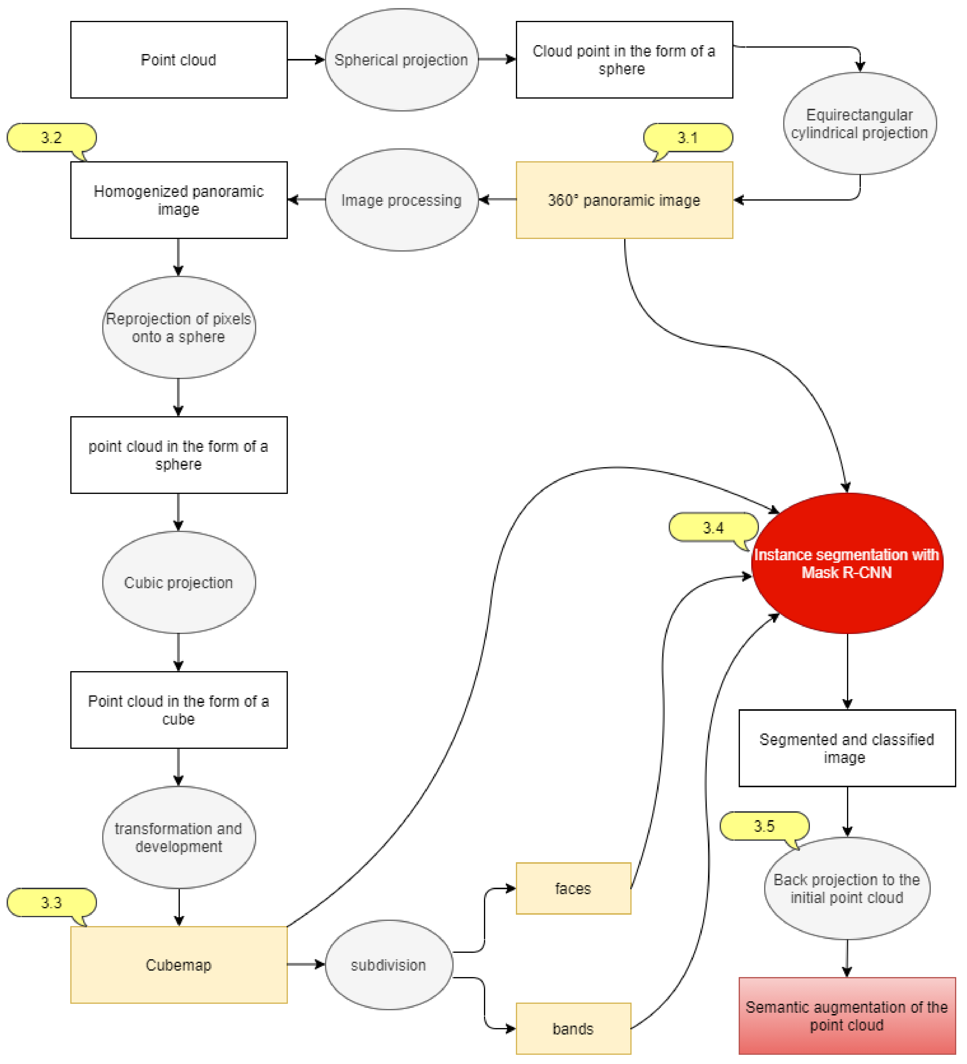
Figure 1. General methodological flowchart.
Remotesensing 13 03647 g001
Figure 2. Schema of the geometry of a spherical projection.
Remotesensing 13 03647 g002
Figure 3. Visualisation on Potree: (a) the initial point cloud; (b) result of the spherical projection. Adapted from ref. [44].
Remotesensing 13 03647 g003
Figure 4. (a) Schema of the equirectangular cylindrical projection; (b) schema of the panoramic image after developing the cylinder (the parallel lines of the sphere are in green and the meridians in red).
Remotesensing 13 03647 g004
Figure 5. (a) Result of the spherical projection visualised on Potree; (b) first panoramic image after the equirectangular cylindrical projection. Adapted from ref. [44].
Remotesensing 13 03647 g005
Figure 6. Panoramic image after applying the two filters.
Remotesensing 13 03647 g006
Figure 7. (a,b) Projection of the 1st region of the sphere on the 1st facet of the cube (plane x = 1).
Remotesensing 13 03647 g007
Figure 8. Projection of the 1st region of the sphere onto the 1st lateral facet of the cube and the two upper and lower facets after applying the condition on coordinate z.
Remotesensing 13 03647 g008
Figure 9. (a) Cube coordinate system before development; (b) cubemap indexing method.
Remotesensing 13 03647 g009
Figure 10. The resulting cubemap of the direct approach.
Remotesensing 13 03647 g010
Figure 11. The resulting cubemap of the inverse approach.
Remotesensing 13 03647 g011
Figure 12. Summarised architecture of the Mask R-CNN Network.
Remotesensing 13 03647 g012
Figure 13. RoIAlign: the dashed grid represents a feature map; the solid lines, an RoI (with 2 × 2 bins in this example); and the dots, the 4 sampling points in each bin. Reprinted from ref. [10].
Remotesensing 13 03647 g013
Figure 14. The 80 object categories in the COCO dataset. Adapted from ref. [48].
Remotesensing 13 03647 g014
Figure 15. (a) Test image; (b) output result of the initial code of the Mask R-CNN instance segmentation network.
Remotesensing 13 03647 g015
Figure 16. Output image keeping only the segmentation masks.
Remotesensing 13 03647 g016
Figure 17. Diagram of the link between the different coordinates tables allowing the back projection of the point with the identifier 10.
Remotesensing 13 03647 g017
Figure 18. Influence of resolution in preserving the informational richness of cloud points.
Remotesensing 13 03647 g018
Figure 19. (a) Chair resolution (786, 1572); (b) chair resolution (3000, 6000); (c) chair resolution (5000, 10,000).
Remotesensing 13 03647 g019
Figure 20. Noise elimination by median filter: (a) before median filter; (b) after median filter.
Remotesensing 13 03647 g020
Figure 21. Noise removal with median filter and the filling of the upper area that had an overabundance of empty pixels: (a) before median filter and filling; (b) after median filter and filling.
Remotesensing 13 03647 g021
Figure 22. Deterioration of the contrast as we increase the size of the median filter: (a) median filter 3 × 3; (b) median filter 7 × 7.
Remotesensing 13 03647 g022
Figure 23. Recovery of writings on papers: (a) before image processing; (b) after image processing.
Remotesensing 13 03647 g023
Figure 24. Influence of the projection centre position on the segmentation of the point cloud.
Remotesensing 13 03647 g024
Figure 25. Influence of the panoramic image resolution on the cloud segmentation rate: (a) almost half of the points representing the two objects were not segmented; (b) almost all the points representing the two objects have been segmented.
Remotesensing 13 03647 g025
Figure 26. Influence of the scattered structure of the point cloud.
Remotesensing 13 03647 g026
Figure 27. Instance segmentation on different point cloud panoramic images: (a) Office point cloud; (b) Female Statue point cloud; (c) Bed point cloud; (d) Boardroom point cloud.
Remotesensing 13 03647 g027
Figure 28. Instance segmentation of the cubemap right facet (the office scene): (a) point cloud; (b) cubemap; (c) instance segmentation on the cubemap right facet.
Remotesensing 13 03647 g028
Figure 29. Examples of the adopted method to calculate quality measures. Blue, red, and green colour represent FN, FP, and TP, respectively.
Remotesensing 13 03647 g029
Figure 30. Generation of panoramic images, Tabkha’s approach on the left and the current approach on the right: (a,b) 360° panoramic image; (c,d) cubemap.
Remotesensing 13 03647 g030
Table 1. Image coordinates of the cubemap facets.
FacetCoordinate iCoordinate j
front A 2 × 3 Z A 2 × 5 + Y
back A 2 × 3 Z A 2 × 3 + Y
left A 2 × 3 Z A 2 × 1 X
right A 2 × 3 Z A 2 × 7 X
top A 2 × 1 + X A 2 × 5 + Y
bottom A 2 × 5 X A 2 × 5 + Y
Table 2. Datasets details.
Point CloudNb of PtsSourceAttributes
Office6,971,911Canon EOS 70D (Photogrammetry)XYZ-RGB
Female Statue3,525,792Leica P30XYZ-RGB-I
Bed3,876,880FARO Focus 3D X330 HDRXYZ-RGB-D
Boardroom30,876,388FARO Focus 3D X330 HDRXYZ-RGB-D
Table 3. Numerical results.
Point CloudObjectPrecisionRecallF1 Score
1#10.7870.9710.869
2#10.9890.9480.968
#10.9520.8990.925
#20.940.8690.903
#30.8640.9860.921
4#40.9690.9450.957
#50.7440.860.798
#60.8740.8950.884
#710.7680.869
#80.9990.7480.855
Average 0.9170.8710.889
Min 0.7440.7480.798
Max 10.9860.957
Table 4. Prediction results of the panoramic image generated by Tabkha’s approach.
ClassPrediction (%)
Interior41
Room27
Modern25
Architecture24
Building22
Device21
Hall20
Seat19.9
Wall19.2
Light18
Table 5. Prediction results of a band extracted from a cubemap generated by the approach of the present study.
ClassPrediction (%)
Room80.28
Interior53.94
furniture50.33
Bedroom48.21
House42.60
Home42.26
Modern29.43
Table28
Design27.56
Floor26.95
Living26.53
Wall26.07
Decor25.63
Chair25.46
Lamp24.97
Sofa23.20
Indoors21.95
Publisher’s Note: MDPI stays neutral with regard to jurisdictional claims in published maps and institutional affiliations.