
A Robust Rigid Registration Framework of 3D Indoor Scene Point Clouds Based on RGB-D Information

 , ,
, , 

Abstract
: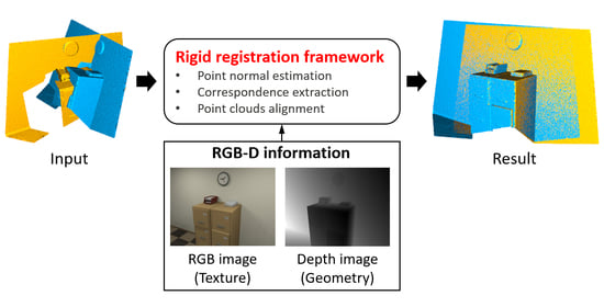
1. Introduction
- We present a point normal estimation method by coupling total variation with second-order variation. The method is capable of effectively removing noise while keeping sharp geometric features and smooth transition regions simultaneously.
- We present a robust correspondence points extraction method, based on a descriptor (TexGeo) encoding both texture and geometry information. With the help of the TexGeo descriptor, the proposed method is robust when handling low-quality point clouds.
- We design a point-to-plane registration method based on a nonconvex regularizer. The method can automatically ignore the influence of those false correspondences and produce an exact rigid transformation between a pair of noisy point clouds.
- We verify the robustness of our approach on a variety of low-quality RGB-D point clouds. Intensive experiments demonstrate that our approach outperforms the selected state-of-the-art methods visually and numerically.
2. Related Work
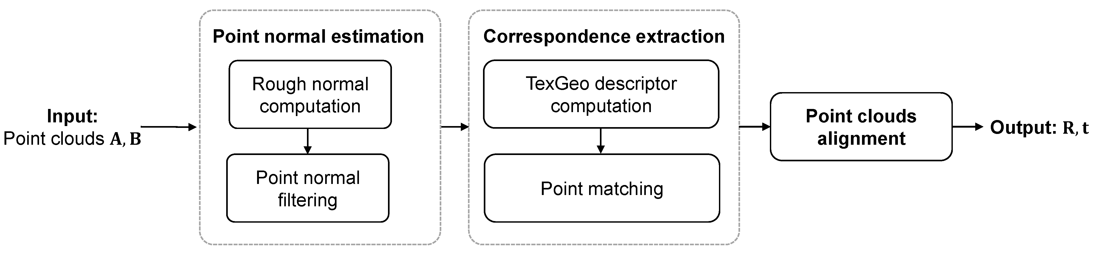
3. Methodology
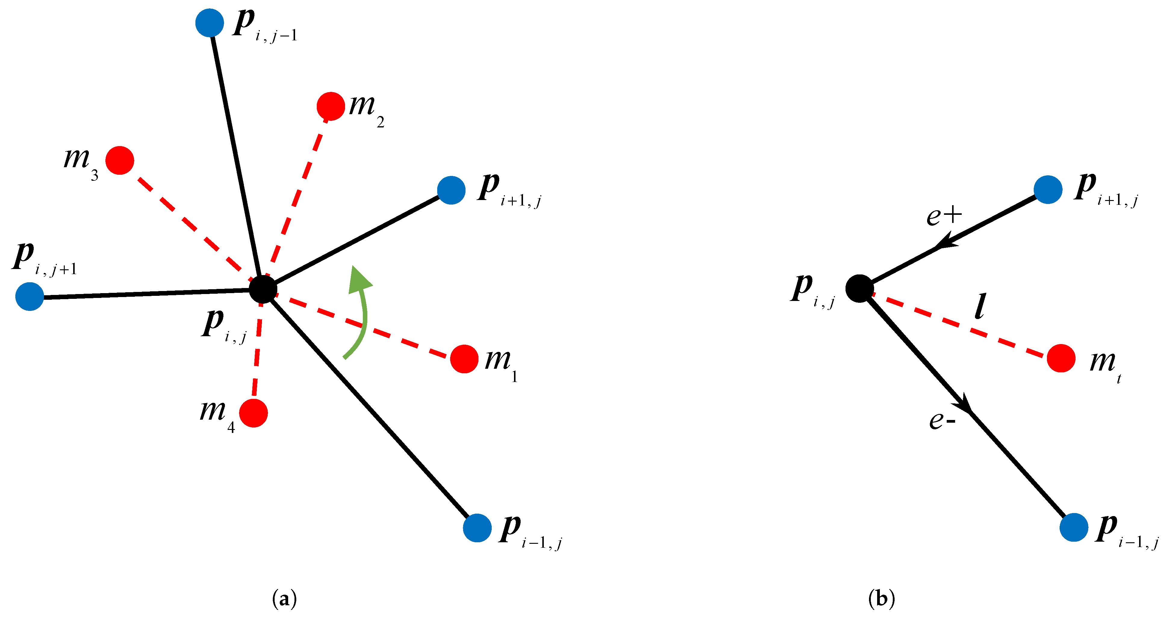
3.1. Point Normal Estimation
| Algorithm 1: The iterative algorithm for minimizing problem (3). |
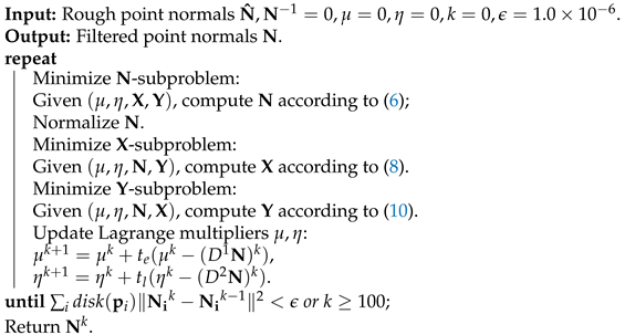 |
3.2. Correspondence Extraction
3.3. Point Clouds Alignment
| Algorithm 2: Robust rigid transformation computation. |
 |
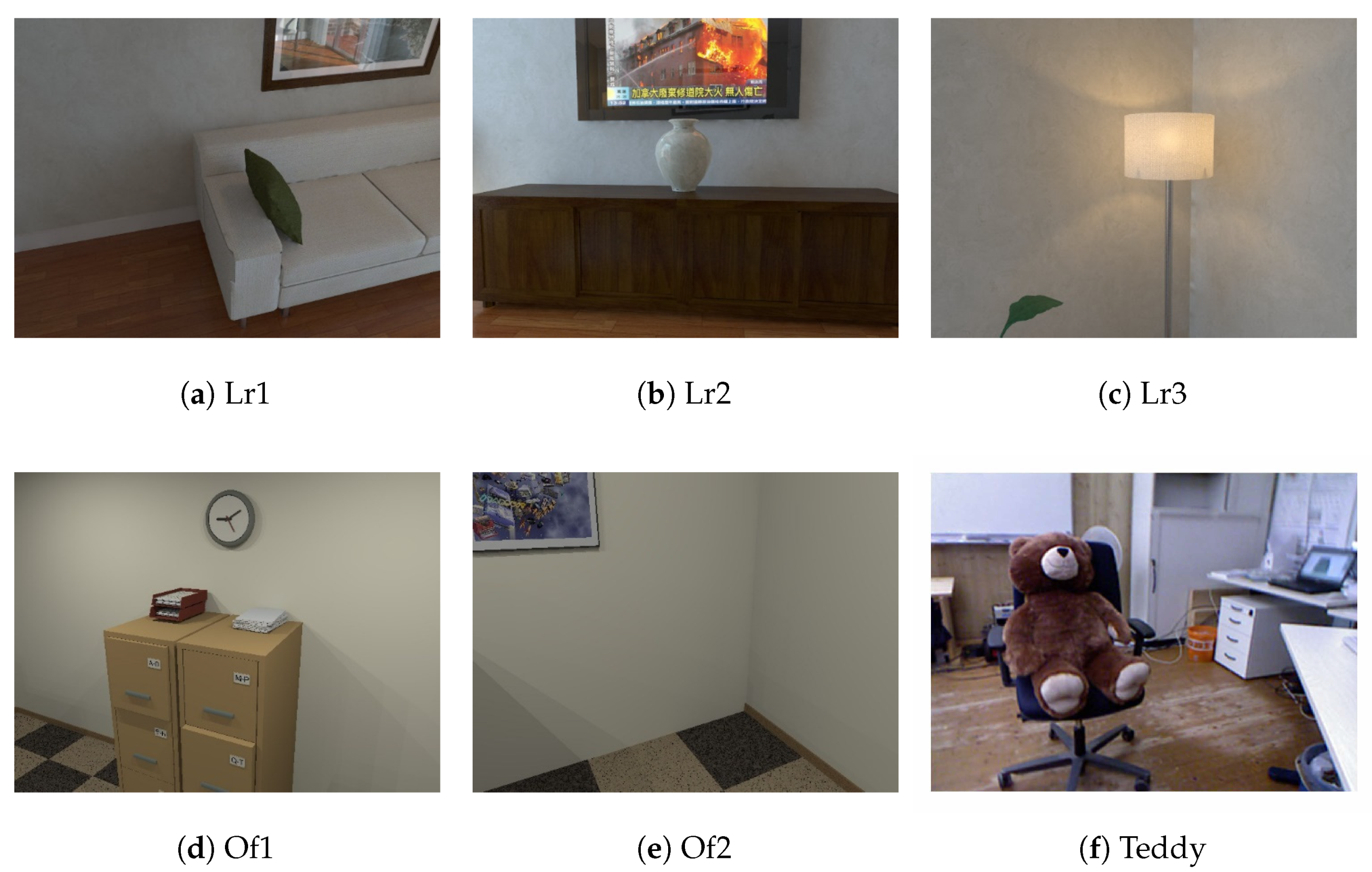
4. Experimental Results
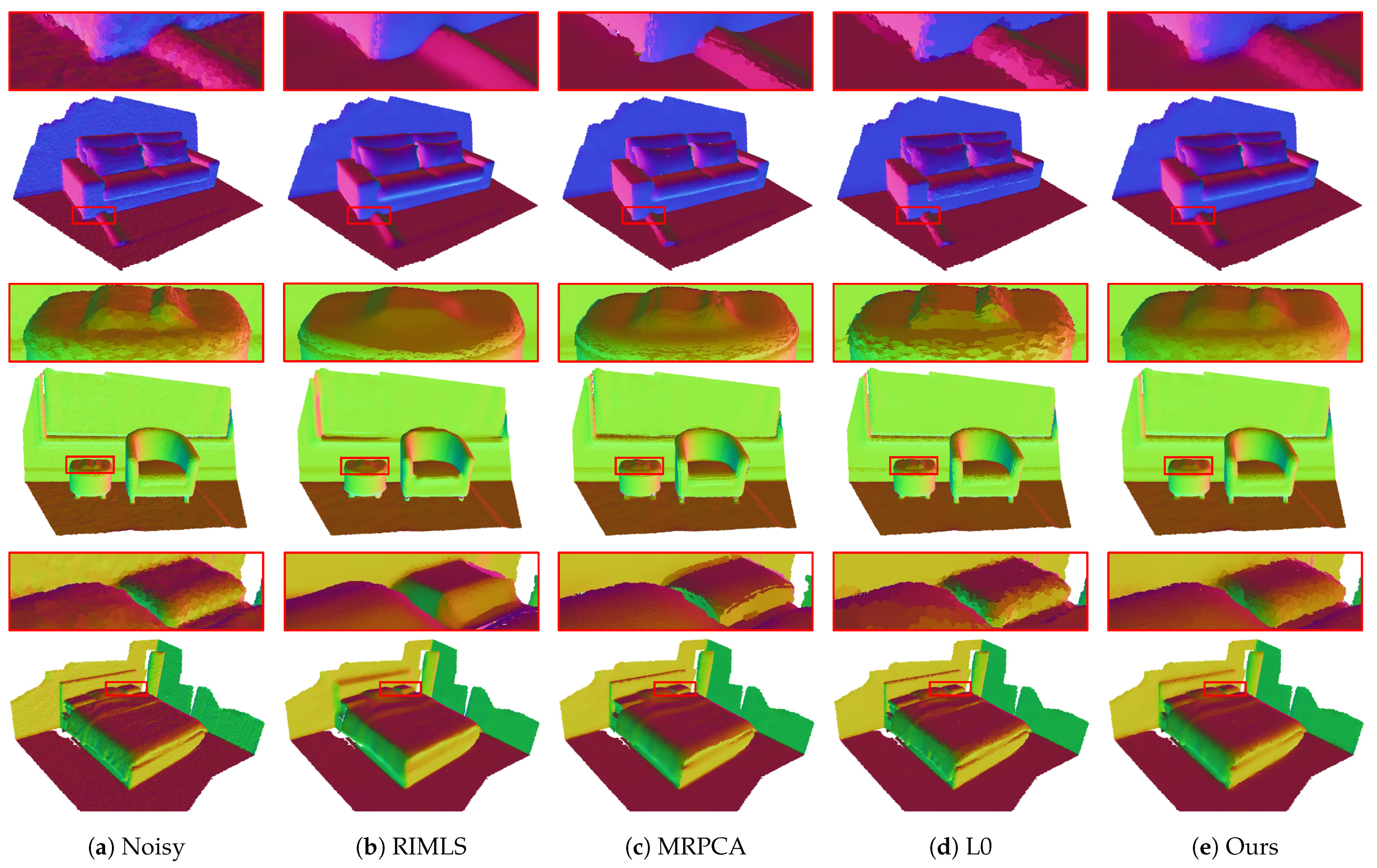
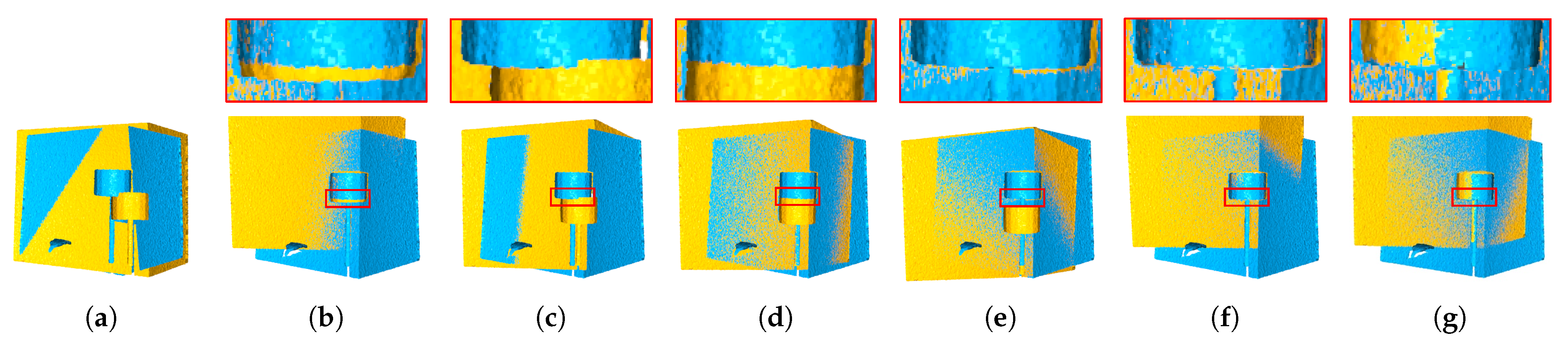
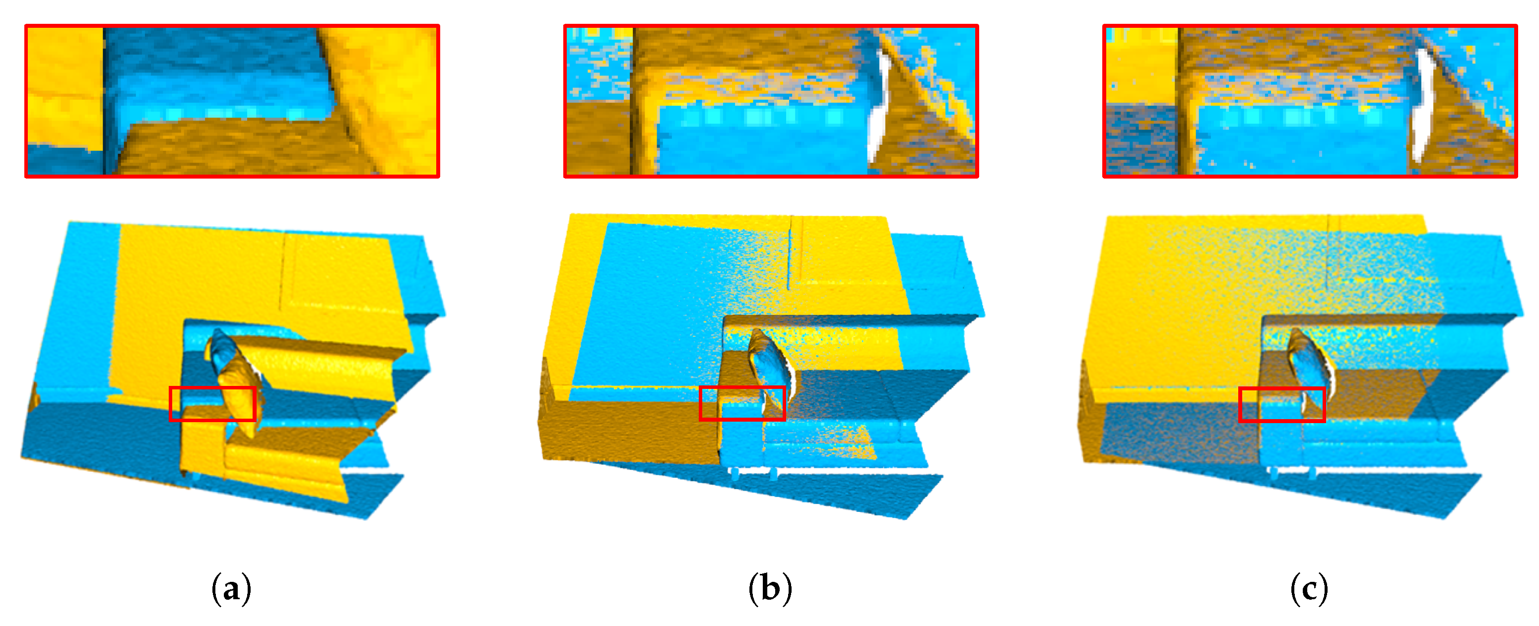
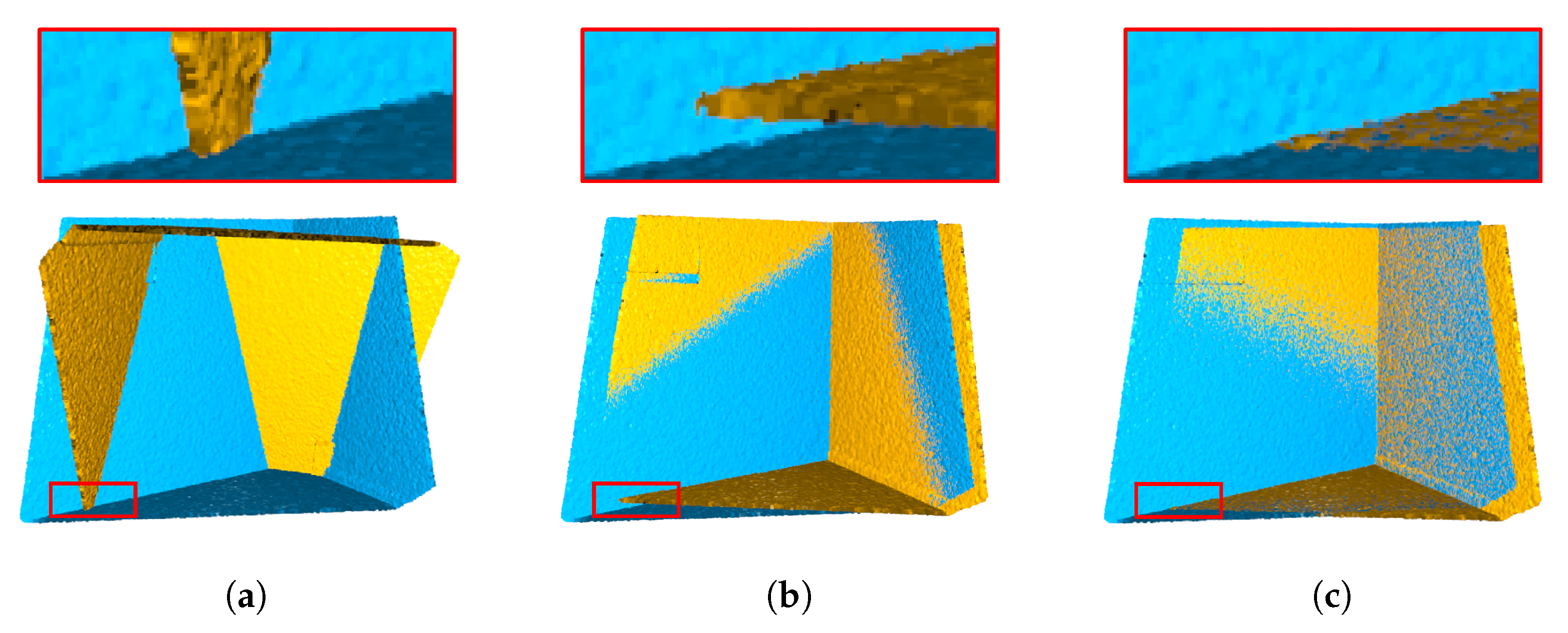
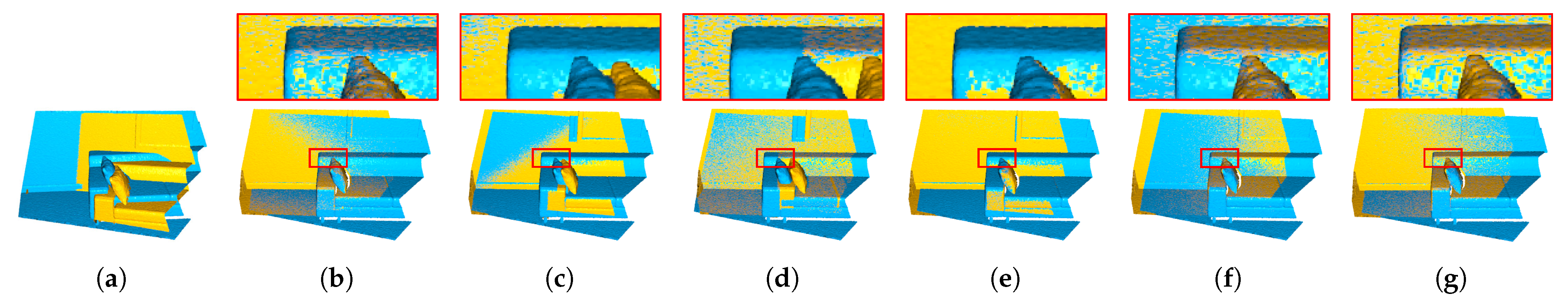
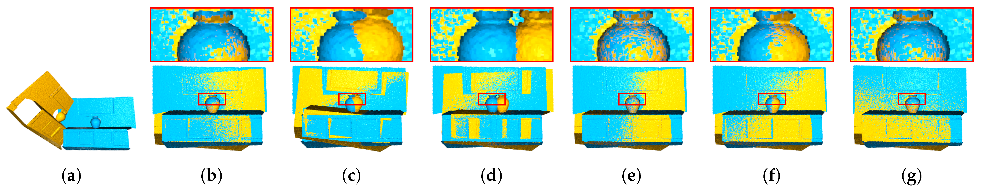
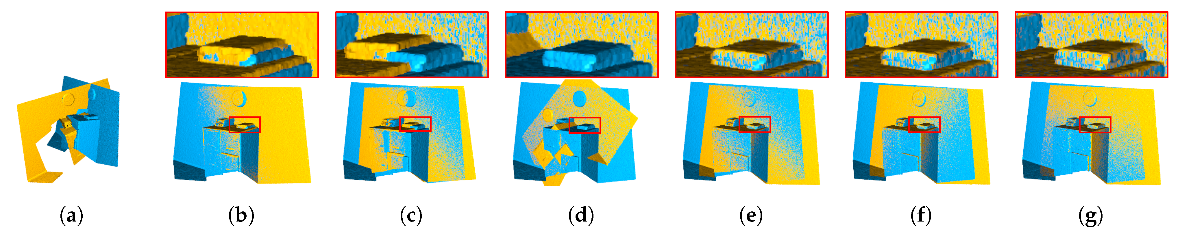
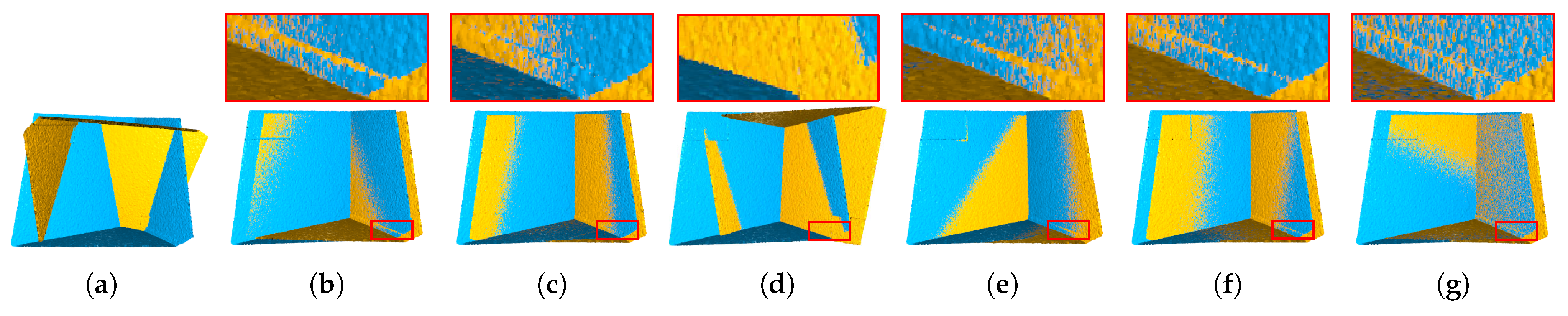
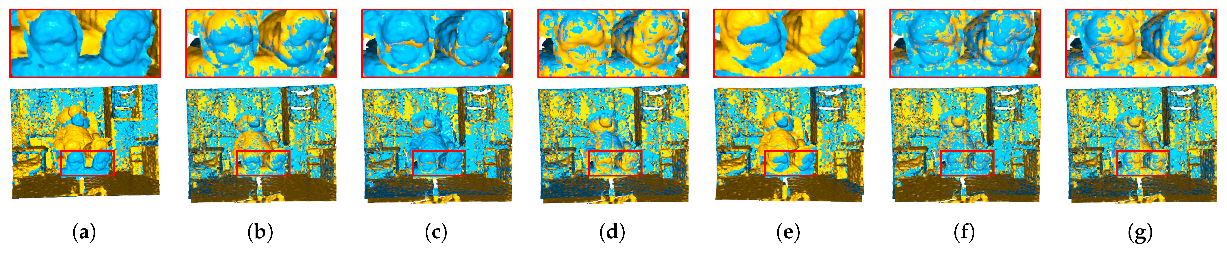
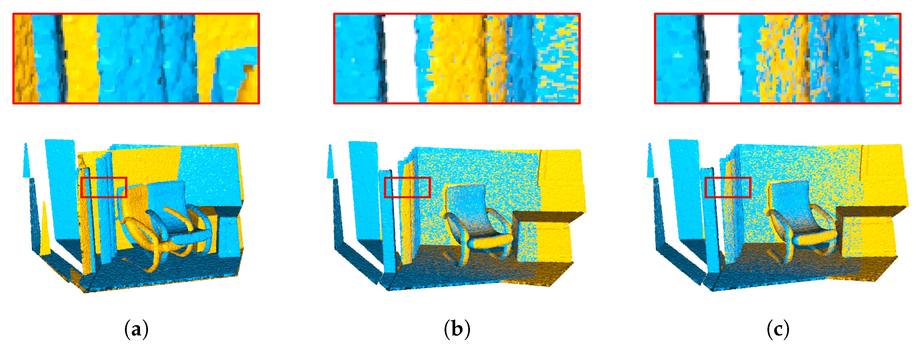
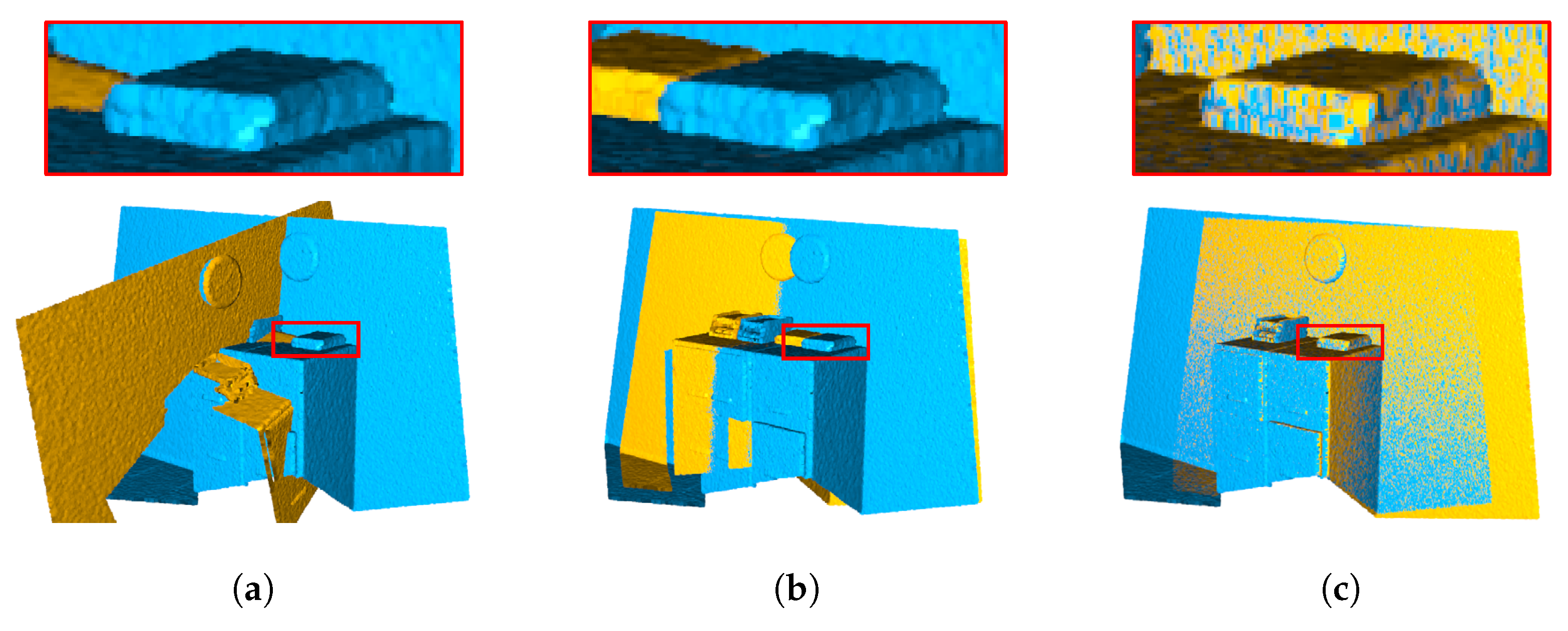
4.1. Qualitative Comparison
4.2. Quantitative Comparison
4.3. Ablation Study
5. Discussion
6. Conclusions
Author Contributions
Funding
Institutional Review Board Statement
Informed Consent Statement
Data Availability Statement
Conflicts of Interest
Abbreviations
| The auxiliary line connecting point with some midpoint | |
| The length of | |
| The area of | |
| The first-order operator | |
| The second-order operator | |
| RIMLS | Robust implicit moving least squares |
| MRPCA | Moving robust principal components analysis |
| L0P | Denoising point sets via minimization |
| PCL | A point cloud library implementation of Rusu et al. [7] |
| S4PCS | Super 4pcs fast global point cloud registration via smart indexing |
| GICP | Go-ICP: a globally optimal solution to 3D ICP point-set registration |
| GICPT | A trimming variant of GICP |
| FGR | Fast global registration |
| SymICP | A symmetric objective function for ICP |
References
- Pavan, N.L.; dos Santos, D.R.; Khoshelham, K. Global registration of terrestrial laser scanner point clouds using plane-to-plane correspondences. Remote Sens. 2020, 12, 1127. [Google Scholar] [CrossRef] [Green Version]
- Cui, Y.; Chang, W.; Nöll, T.; Stricker, D. KinectAvatar: Fully automatic body capture using a single kinect. In Proceedings of the Asian Conference on Computer Vision, Daejeon, Korea, 5–9 November 2012; Springer: Berlin/Heidelberg, Germany, 2012; pp. 133–147. [Google Scholar]
- Globally consistent registration of terrestrial laser scans via graph optimization. ISPRS J. Photogramm. Remote Sens. 2015, 109, 126–138. [CrossRef]
- Besl, P.J.; McKay, N.D. Method for registration of 3-D shapes. In Proceedings of the Sensor Fusion IV: Control Paradigms and data Structures, Boston, MA, USA, 14–15 November 1992; International Society for Optics and Photonics: Bellingham, WA, USA, 1992; Volume 1611, pp. 586–606. [Google Scholar]
- Newcombe, R.A.; Izadi, S.; Hilliges, O.; Molyneaux, D.; Kim, D.; Davison, A.J.; Kohi, P.; Shotton, J.; Hodges, S.; Fitzgibbon, A. KinectFusion: Real-time dense surface mapping and tracking. In Proceedings of the 2011 10th IEEE International Symposium on Mixed and Augmented Reality, Basel, Switzerland, 26–29 October 2011; pp. 127–136. [Google Scholar]
- Rusinkiewicz, S.; Levoy, M. Efficient variants of the ICP algorithm. In Proceedings of the Third International Conference on 3-D Digital Imaging and Modeling, Quebec City, QC, Canada, 28 May–1 June 2001; pp. 145–152. [Google Scholar]
- Rusu, R.B.; Blodow, N.; Beetz, M. Fast point feature histograms (FPFH) for 3D registration. In Proceedings of the 2009 IEEE International Conference on Robotics and Automation, Kobe, Japan, 12–17 May 2009; pp. 3212–3217. [Google Scholar]
- Gelfand, N.; Mitra, N.J.; Guibas, L.J.; Pottmann, H. Robust Global Registration. In Proceedings of the Third Eurographics Symposium on Geometry Processing, Vienna, Austria, 4–6 July 2005. [Google Scholar]
- Takimoto, R.Y.; Tsuzuki, M.d.S.G.; Vogelaar, R.; de Castro Martins, T.; Sato, A.K.; Iwao, Y.; Gotoh, T.; Kagei, S. 3D reconstruction and multiple point cloud registration using a low precision RGB-D sensor. Mechatronics 2016, 35, 11–22. [Google Scholar] [CrossRef]
- Endres, F.; Hess, J.; Engelhard, N.; Sturm, J.; Cremers, D.; Burgard, W. An evaluation of the RGB-D SLAM system. In Proceedings of the 2012 IEEE International Conference on Robotics and Automation, Saint Paul, MN, USA, 14–18 May 2012; pp. 1691–1696. [Google Scholar]
- Henry, P.; Krainin, M.; Herbst, E.; Ren, X.; Fox, D. RGB-D mapping: Using depth cameras for dense 3D modeling of indoor environments. In Experimental Robotics; Springer: Berlin/Heidelberg, Germany, 2014; pp. 477–491. [Google Scholar]
- Guo, M.; Wu, L.; Huang, Y.; Chen, X. An efficient internet map tiles rendering approach on high resolution devices. J. Spat. Sci. 2021, 1–19. [Google Scholar] [CrossRef]
- Wan, T.; Du, S.; Cui, W.; Yang, Y.; Li, C. Robust Rigid Registration Algorithm Based on Correntropy and Bi-Directional Distance. IEEE Access 2020, 8, 22225–22234. [Google Scholar] [CrossRef]
- Wan, T.; Du, S.; Cui, W.; Yao, R.; Ge, Y.; Li, C.; Gao, Y.; Zheng, N. RGB-D Point Cloud Registration Based on Salient Object Detection. IEEE Trans. Neural Netw. Learn. Syst. 2021, 1–13. [Google Scholar] [CrossRef] [PubMed]
- Aiger, D.; Mitra, N.J.; Cohen-Or, D. 4-points congruent sets for robust pairwise surface registration. ACM Trans. Graph. 2008, 27, 1–10. [Google Scholar] [CrossRef] [Green Version]
- Chen, S.; Nan, L.; Xia, R.; Zhao, J.; Wonka, P. PLADE: A plane-based descriptor for point cloud registration with small overlap. IEEE Trans. Geosci. Remote Sens. 2019, 58, 2530–2540. [Google Scholar] [CrossRef]
- Zhang, L.; Guo, J.; Cheng, Z.; Xiao, J.; Zhang, X. Efficient Pairwise 3-D Registration of Urban Scenes via Hybrid Structural Descriptors. IEEE Trans. Geosci. Remote. Sens. 2021, 1–17. [Google Scholar] [CrossRef]
- Bylow, E.; Sturm, J.; Kerl, C.; Kahl, F.; Cremers, D. Real-time camera tracking and 3D reconstruction using signed distance functions. In Robotics: Science and systems (RSS); Robotics: Science and Systems: Berlin, Germany, 2013; Volume 2, p. 2. [Google Scholar]
- Pavlov, A.L.; Ovchinnikov, G.W.; Derbyshev, D.Y.; Tsetserukou, D.; Oseledets, I.V. AA-ICP: Iterative closest point with Anderson acceleration. In Proceedings of the 2018 IEEE International Conference on Robotics and Automation (ICRA), Brisbane, Australia, 21–25 May 2018; pp. 3407–3412. [Google Scholar]
- Zhang, J.; Yao, Y.; Deng, B. Fast and Robust Iterative Closest Point. IEEE Trans. Pattern Anal. Mach. Intell. 2021, 1. [Google Scholar] [CrossRef] [PubMed]
- Chetverikov, D.; Stepanov, D.; Krsek, P. Robust Euclidean alignment of 3D point sets: The trimmed iterative closest point algorithm. Image Vis. Comput. 2005, 23, 299–309. [Google Scholar] [CrossRef]
- Bouaziz, S.; Tagliasacchi, A.; Pauly, M. Sparse iterative closest point. In Computer Graphics Forum; Wiley Online Library: Hoboken, NJ, USA, 2013; Volume 32, pp. 113–123. [Google Scholar]
- Zhou, Q.Y.; Park, J.; Koltun, V. Fast global registration. In Proceedings of the European Conference on Computer Vision, Amsterdam, The Netherlands, 8–16 October 2016; Springer: Berlin/Heidelberg, Germany, 2016; pp. 766–782. [Google Scholar]
- Wu, Z.; Chen, H.; Du, S.; Fu, M.; Zhou, N.; Zheng, N. Correntropy based scale ICP algorithm for robust point set registration. Pattern Recognit. 2019, 93, 14–24. [Google Scholar] [CrossRef]
- Yang, J.; Li, H.; Jia, Y. Go-icp: Solving 3d registration efficiently and globally optimally. In Proceedings of the IEEE International Conference on Computer Vision, Sydney, Australia, 1–8 December 2013; pp. 1457–1464. [Google Scholar]
- Feng, W.; Zhang, J.; Cai, H.; Xu, H.; Hou, J.; Bao, H. Recurrent Multi-view Alignment Network for Unsupervised Surface Registration. In Proceedings of the IEEE/CVF Conference on Computer Vision and Pattern Recognition, Nashville, TN, USA, 19–25 June 2021; pp. 10297–10307. [Google Scholar]
- Li, X.; Pontes, J.K.; Lucey, S. PointNetLK Revisited. In Proceedings of the IEEE/CVF Conference on Computer Vision and Pattern Recognition, Nashville, TN, USA, 19–25 June 2021; pp. 12763–12772. [Google Scholar]
- Wang, Y.; Solomon, J.M. Deep closest point: Learning representations for point cloud registration. In Proceedings of the IEEE/CVF International Conference on Computer Vision, Seoul, Korea, 27–28 October 2019; pp. 3523–3532. [Google Scholar]
- Guo, M.; Liu, H.; Xu, Y.; Huang, Y. Building extraction based on U-Net with an attention block and multiple losses. Remote Sens. 2020, 12, 1400. [Google Scholar] [CrossRef]
- Guo, M.; Yu, Z.; Xu, Y.; Huang, Y.; Li, C. ME-Net: A Deep Convolutional Neural Network for Extracting Mangrove Using Sentinel-2A Data. Remote Sens. 2021, 13, 1292. [Google Scholar] [CrossRef]
- Tam, G.K.; Cheng, Z.Q.; Lai, Y.K.; Langbein, F.C.; Liu, Y.; Marshall, D.; Martin, R.R.; Sun, X.F.; Rosin, P.L. Registration of 3D point clouds and meshes: A survey from rigid to nonrigid. IEEE Trans. Vis. Comput. Graph. 2012, 19, 1199–1217. [Google Scholar] [CrossRef] [Green Version]
- Avron, H.; Sharf, A.; Greif, C.; Cohen-Or, D. ℓ1-sparse reconstruction of sharp point set surfaces. ACM Trans. Graph. TOG 2010, 29, 1–12. [Google Scholar] [CrossRef]
- Sun, Y.; Schaefer, S.; Wang, W. Denoising point sets via L0 minimization. Comput. Aided Geom. Des. 2015, 35–36, 2–15. [Google Scholar] [CrossRef]
- Zhong, S.; Xie, Z.; Wang, W.; Liu, Z.; Liu, L. Mesh denoising via total variation and weighted Laplacian regularizations. Comput. Animat. Virtual Worlds 2018, 29, e1827. [Google Scholar] [CrossRef]
- Zhong, S.; Xie, Z.; Liu, J.; Liu, Z. Robust Mesh Denoising via Triple Sparsity. Sensors 2019, 19, 1001. [Google Scholar] [CrossRef] [Green Version]
- Liu, Z.; Zhong, S.; Xie, Z.; Wang, W. A novel anisotropic second order regularization for mesh denoising. Comput. Aided Geom. Des. 2019, 71, 190–201. [Google Scholar] [CrossRef]
- Liu, Z.; Wang, W.; Zhong, S.; Zeng, B.; Liu, J.; Wang, W. Mesh Denoising via a Novel Mumford–Shah Framework. Comput. Aided Des. 2020, 126, 102858. [Google Scholar] [CrossRef]
- Guo, M.; Song, Z.; Han, C.; Zhong, S.; Lv, R.; Liu, Z. Mesh denoising via adaptive consistent neighborhood. Sensors 2021, 21, 412. [Google Scholar] [CrossRef] [PubMed]
- Zhong, S.; Song, Z.; Liu, Z.; Xie, Z.; Chen, J.; Liu, L.; Chen, R. Shape-aware Mesh Normal Filtering. Comput. Aided Des. 2021, 140, 103088. [Google Scholar] [CrossRef]
- Liu, Z.; Li, Y.; Wang, W.; Liu, L.; Chen, R. Mesh Total Generalized Variation for Denoising. IEEE Trans. Vis. Comput. Graph. 2021, 1. [Google Scholar] [CrossRef] [PubMed]
- Liu, Z.; Xiao, X.; Zhong, S.; Wang, W.; Li, Y.; Zhang, L.; Xie, Z. A feature-preserving framework for point cloud denoising. Comput. Aided Des. 2020, 127, 102857. [Google Scholar] [CrossRef]
- Raguram, R.; Frahm, J.M.; Pollefeys, M. A comparative analysis of RANSAC techniques leading to adaptive real-time random sample consensus. In Proceedings of the European Conference on Computer Vision, Marseille, France, 12–18 October 2008; Springer: Berlin/Heidelberg, Germany, 2008; pp. 500–513. [Google Scholar]
- Fischler, M.A.; Bolles, R.C. Random sample consensus: A paradigm for model fitting with applications to image analysis and automated cartography. Commun. ACM 1981, 24, 381–395. [Google Scholar] [CrossRef]
- Mellado, N.; Aiger, D.; Mitra, N.J. Super 4pcs fast global pointcloud registration via smart indexing. In Computer Graphics Forum; Wiley Online Library: Hoboken, NJ, USA, 2014; Volume 33, pp. 205–215. [Google Scholar]
- Mavridis, P.; Andreadis, A.; Papaioannou, G. Efficient Sparse Icp. Comput. Aided Geom. Des. 2015, 35, 16–26. [Google Scholar] [CrossRef]
- Rusinkiewicz, S. A symmetric objective function for ICP. ACM Trans. Graph. TOG 2019, 38, 1–7. [Google Scholar] [CrossRef]
- Diebel, J. Representing attitude: Euler angles, unit quaternions, and rotation vectors. Matrix 2006, 58, 1–35. [Google Scholar]
- Pan, H.; Guan, T.; Luo, Y.; Duan, L.; Tian, Y.; Yi, L.; Zhao, Y.; Yu, J. Dense 3D reconstruction combining depth and RGB information. Neurocomputing 2016, 175, 644–651. [Google Scholar] [CrossRef]
- Handa, A.; Whelan, T.; McDonald, J.; Davison, A.J. A benchmark for RGB-D visual odometry, 3D reconstruction and SLAM. In Proceedings of the 2014 IEEE International Conference on Robotics and Automation (ICRA), Hong Kong, China, 31 May–7 June 2014; pp. 1524–1531. [Google Scholar]
- Dai, W.; Zhang, Y.; Li, P.; Fang, Z.; Scherer, S. RGB-D SLAM in Dynamic Environments Using Point Correlations. IEEE Trans. Pattern Anal. Mach. Intell. 2020, 1. [Google Scholar] [CrossRef]
- Sipiran, I.; Bustos, B. Harris 3D: A robust extension of the Harris operator for interest point detection on 3D meshes. Vis. Comput. 2011, 27, 963–976. [Google Scholar] [CrossRef]
- Wang, P.S.; Liu, Y.; Tong, X. Mesh Denoising via Cascaded Normal Regression. ACM Trans. Graph. 2016, 35, 232:1–232:12. [Google Scholar] [CrossRef]
- Öztireli, A.C.; Guennebaud, G.; Gross, M. Feature preserving point set surfaces based on non-linear kernel regression. In Computer Graphics Forum; Wiley Online Library: Hoboken, NJ, USA, 2009; Volume 28, pp. 493–501. [Google Scholar]
- Mattei, E.; Castrodad, A. Point cloud denoising via moving RPCA. In Computer Graphics Forum; Wiley Online Library: Hoboken, NJ, USA, 2017; Volume 36, pp. 123–137. [Google Scholar]
- Bay, H.; Tuytelaars, T.; Van Gool, L. Surf: Speeded up robust features. In Proceedings of the European Conference on Computer Vision, Graz, Austria, 7–13 May 2006; Springer: Berlin/Heidelberg, Germany, 2006; pp. 404–417. [Google Scholar]
- Black, M.J.; Rangarajan, A. On the unification of line processes, outlier rejection, and robust statistics with applications in early vision. Int. J. Comput. Vis. 1996, 19, 57–91. [Google Scholar] [CrossRef]
- Park, J.; Zhou, Q.Y.; Koltun, V. Colored Point Cloud Registration Revisited. In Proceedings of the 2017 IEEE International Conference on Computer Vision (ICCV), Venice, Italy, 22–29 October 2017; pp. 143–152. [Google Scholar]
- Yang, J.; Li, H.; Campbell, D.; Jia, Y. Go-ICP: A globally optimal solution to 3D ICP point-set registration. IEEE Trans. Pattern Anal. Mach. Intell. 2015, 38, 2241–2254. [Google Scholar] [CrossRef] [PubMed] [Green Version]
- Handa, A.; Whelan, T.; McDonald, J.B.; Davison, A.J. The ICL-NUIM Dataset. 2014. Available online: http://www.doc.ic.ac.uk/~ahanda/VaFRIC/iclnuim.html (accessed on 23 September 2021).
- Sturm, J.; Engelhard, N.; Endres, F.; Burgard, W.; Cremers, D. The TUM Dataset. 2012. Available online: https://vision.in.tum.de/data/datasets/rgbd-dataset/download (accessed on 23 September 2021).


| Point Clouds | ||||||
|---|---|---|---|---|---|---|
| PCL | GICP | GICPT | S4PCS | FGR | Our Approach | |
| Lr1 | 2.800 | 4.791 | 2.658 | 4.275 | 2.614 | 2.526 |
| Lr2 | 3.067 | 4.747 | 3.691 | 3.566 | 2.917 | 2.613 |
| Lr3 | 4.485 | 5.509 | 3.352 | 3.492 | 3.614 | 3.202 |
| Of1 | 3.006 | 2.715 | 3.049 | 2.218 | 2.070 | 1.869 |
| Of2 | 5.013 | 4.584 | 5.547 | 5.043 | 4.283 | 3.935 |
| Teddy | 5.893 | 6.356 | 5.767 | 6.545 | 5.710 | 5.661 |
Publisher’s Note: MDPI stays neutral with regard to jurisdictional claims in published maps and institutional affiliations. |
© 2021 by the authors. Licensee MDPI, Basel, Switzerland. This article is an open access article distributed under the terms and conditions of the Creative Commons Attribution (CC BY) license (https://creativecommons.org/licenses/by/4.0/).
Share and Cite
Zhong, S.; Guo, M.; Lv, R.; Chen, J.; Xie, Z.; Liu, Z. A Robust Rigid Registration Framework of 3D Indoor Scene Point Clouds Based on RGB-D Information. Remote Sens. 2021, 13, 4755. https://doi.org/10.3390/rs13234755
Zhong S, Guo M, Lv R, Chen J, Xie Z, Liu Z. A Robust Rigid Registration Framework of 3D Indoor Scene Point Clouds Based on RGB-D Information. Remote Sensing. 2021; 13(23):4755. https://doi.org/10.3390/rs13234755
Chicago/Turabian StyleZhong, Saishang, Mingqiang Guo, Ruina Lv, Jianguo Chen, Zhong Xie, and Zheng Liu. 2021. "A Robust Rigid Registration Framework of 3D Indoor Scene Point Clouds Based on RGB-D Information" Remote Sensing 13, no. 23: 4755. https://doi.org/10.3390/rs13234755
APA StyleZhong, S., Guo, M., Lv, R., Chen, J., Xie, Z., & Liu, Z. (2021). A Robust Rigid Registration Framework of 3D Indoor Scene Point Clouds Based on RGB-D Information. Remote Sensing, 13(23), 4755. https://doi.org/10.3390/rs13234755