1. Introduction
A synthetic aperture radar (SAR) can provide continuous observation of objects on the Earth’s surface, something which has been extensively studied in a large body of object detection work [
1]. With the improving resolution of acquired SAR images, aircraft detection is beginning to be more widely-adopted in advanced image analytics studies [
2]. The challenge of aircraft detection lies in the increasing data volume, the interference of complex backgrounds, and scattered image features of aircraft as objects for detection [
3]. Among various SAR image analytical methods, machine learning approaches have attracted considerable interest due to their high accuracy and ability to automatically process large volumes of SAR imagery [
4].
Deep neural networks (DNN), an advanced machine learning method inspired by the structure and function of the brain system, have been extensively employed in recent developments of object detection from remotely sensed imagery [
5,
6]. Numerous DNNs have been explored for use in aircraft detection. Convolutional neural networks (CNN) were adopted to achieve accurate aircraft detection results in [
7]. Tan et al. [
8] designed a DNN based on attention mechanisms for airport detection. Based on this work, Wang et al. [
2] integrated weighted feature fusion with attention mechanisms, to implement high-precision aircraft detection by combining the airport mask. New DNN structures are being continuously proposed and their complexity is growing correspondingly [
9].
Most DNN approaches have, however, been criticized for their blackbox behaviors [
10], something that makes exploration of advanced deep learning approaches such as attention mechanisms and data augmentation techniques more difficult [
11]. High accuracy alone is often insufficient to evaluate the performance of a given DNN, with the extent to which the functioning of DNN can be understood by users becoming increasingly important [
10].
Methods called eXplainable Artificial Intelligence (XAI) begin to reveal which feature or neurons are important and at which stage of the image analytics they are important. XAI can provide insights into the inner functioning of DNN, to enhance the understandability, transparency, traceability, causality and trust in the employment of DNN [
12]. Mandeep et al. [
13] justified the results of deep learning-based target classification using SAR images. Nonetheless, XAI has not yet been investigated for DNN-based target detection.
To fill this gap, we propose an innovative XAI framework to glassbox DNN in SAR image analytics, which offers the selection of optimal backbone network architecture and visual interpretation of object detection performance. Our XAI framework is designed for aircraft detection initially but will be extended to other object detection tasks in our future work. The contribution of this paper can be summarized as:
- (1)
We propose a new hybrid XAI algorithm to explain DNN, by combining local integrated gradients [
14] and the global attribution mapping [
15] methods. This hybrid XAI method is named hybrid global attribution mapping (HGAM), which provides comprehensive metrics to assess the object detection performance of DNN.
- (2)
An innovative XAI visualization method called class-specific confidence scores mapping (CCSM) is designed and developed as an effective approach for visual understanding of the detection head performance. CCSM highlights pivotal information about the decision-making of aircraft detection from feature maps generated by DNN.
- (3)
By combining the hybrid XAI algorithm and the metrics of CCSM, we propose an innovative workflow to glassbox DNN with high understandability. This workflow does not only select the most suitable backbone DNN, but also offers an explanatory approach to the effectiveness of feature extraction and object detection with given input datasets.
The rest of this paper is organized as follows. We highlight the necessity of employing XAI within deep learning techniques for aircraft detection in
Section 2. The methodology of our proposed XAI framework is outlined in
Section 3. Experiments using Geofen-3 imagery for aircraft detection are presented in
Section 4; while findings are discussed in
Section 5. Finally, we conclude in
Section 6.
2. Problem Statement
Although DNN has been shown to be successful in automatic aircraft detection [
2], its blackbox behaviors have impeded the understandability and wider application of DNN in SAR image analytics. Therefore, we need to glassbox DNN not only to understand its feature extraction and decision-making processes, but also obtain more insights about the selection of backbone networks for the design and development of DNN.
To the best of our knowledge, this is the first work employing XAI in object detection from SAR imagery. There are some initial XAI works in geospatial image analytics but these have not yet been extended to aircraft detection. Guo et al. [
16] utilized XAI to gain clues for network pruning in CNN, but their case studies only consider optical remotely-sensed imagery in land-use classification. Abdollahi and Pradhan [
17] conducted feature selection based on SHapley Additive exPlanations (SHAP) [
18] with aerial photos. SHAP was also used in [
19], but with Landsat-7 images for building damage classification. We note XAI techniques in these works are all for classification studies, not for object detection.
When we employ XAI for aircraft detection, the foremost challenge comes from the coordination of local and global XAI techniques towards the determination of backbone networks. Local XAI focuses on explaining the feature extraction attribution of each layer in DNN with a given input image; while global XAI usually brings better understandability of the overall DNN model. It is important to avoid selecting a backbone network with good object detection performance but poor performance in feature extraction, and it becomes very necessary to consider the integration of local and global approaches as hybrid XAI methods for the determination of backbone networks.
Another challenge lies in the customization of XAI techniques for object detection in SAR image analytics, because most of these techniques have been designed for classification [
20]. In contrast to such classification tasks, DNN in the object detection task is used to locate and classify (usually multiple) targets in the input images. Thus, we need to explain the object detection results along with their location information. At present, the combination of the internal classification results and location information of objects is the topic of a number of XAI studies.
A third challenge arises from the fact that the feature extraction performance of detection heads is not understandable, and we still lack an effective metric to depict such attribution of feature extraction. The performance of detection heads plays a pivotal role in object detection, with high contribution to the final object detection results [
21]. Therefore, we need to understand their behaviors, and a visual interpretation would improve that understanding.
To address these research challenges, we combine local and global XAI methods to design and develop a hybrid XAI specifically for explaining object detection in SAR image analytics. At the same time, we also propose our own visualization method to depict the attribution of detection heads towards the final object detection results.
3. Methodology
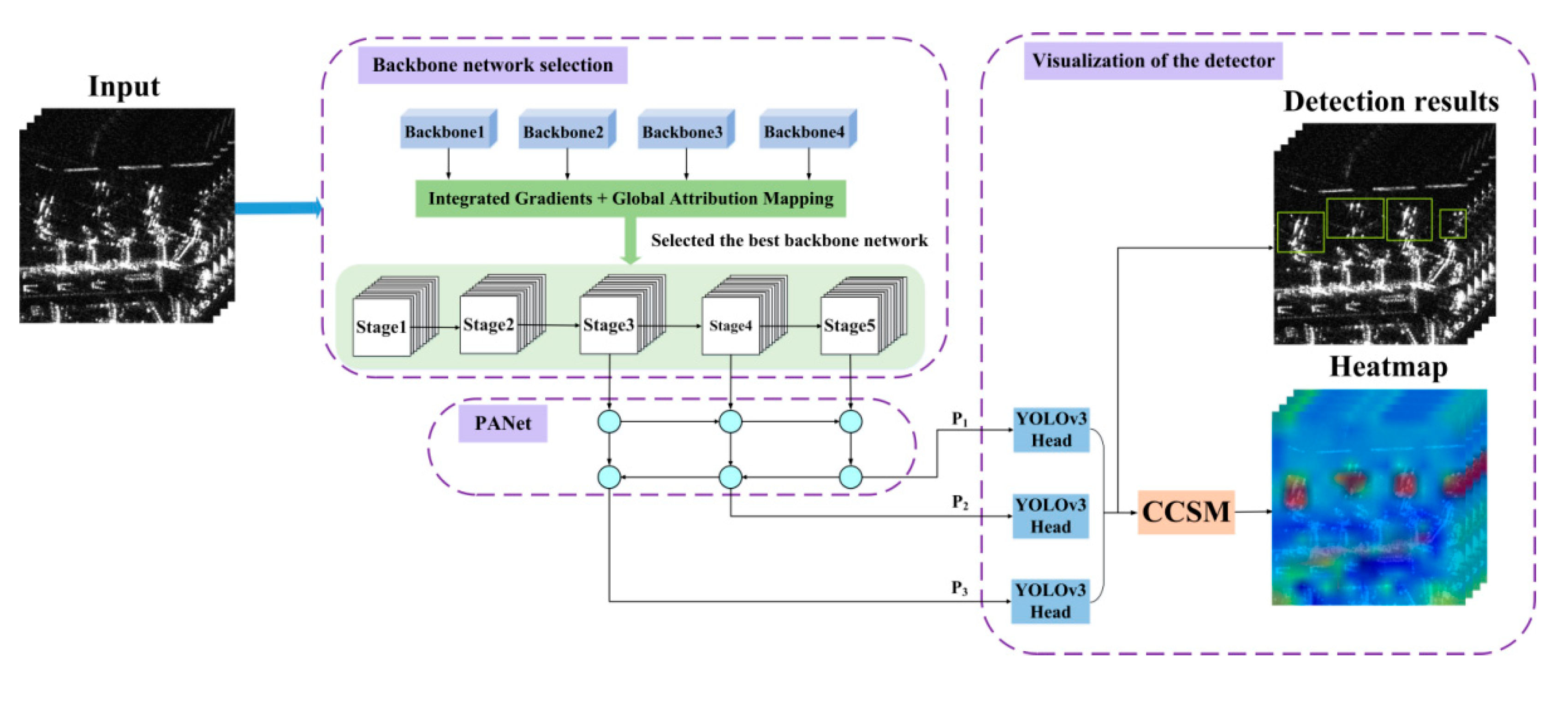
3.1. Overall Methodology Framework
By combining SAR image analytics with XAI methods, an innovative XAI framework for target detection from SAR images is proposed in this paper. The architecture of the proposed XAI framework is composed of three parts: backbone network selection, Path Aggregation Network (PANet) [
22], and visualization of the detector, as shown in
Figure 1.
First, different backbone networks are trained using SAR imagery datasets containing aircraft with 1 m resolution from the Gaofen-3 system, and the optimal weight model is retained. Then, HGAM is used to analyze each backbone network, and the optimal one with the best classification results is selected to extract feature maps of aircraft. HGAM is a new method proposed in this paper, which is composed of integrated gradients (IG) [
14] and global attribution mapping (GAM) [
15] (see
Section 3.2. for details). Furthermore, the PANet is introduced to fuse the feature maps (with different resolutions and receptive fields) output by the last three stages of the backbone network to enrich the expression of features. After the feature maps are enhanced by the PANet module, they are input into the YOLOv3 detection head [
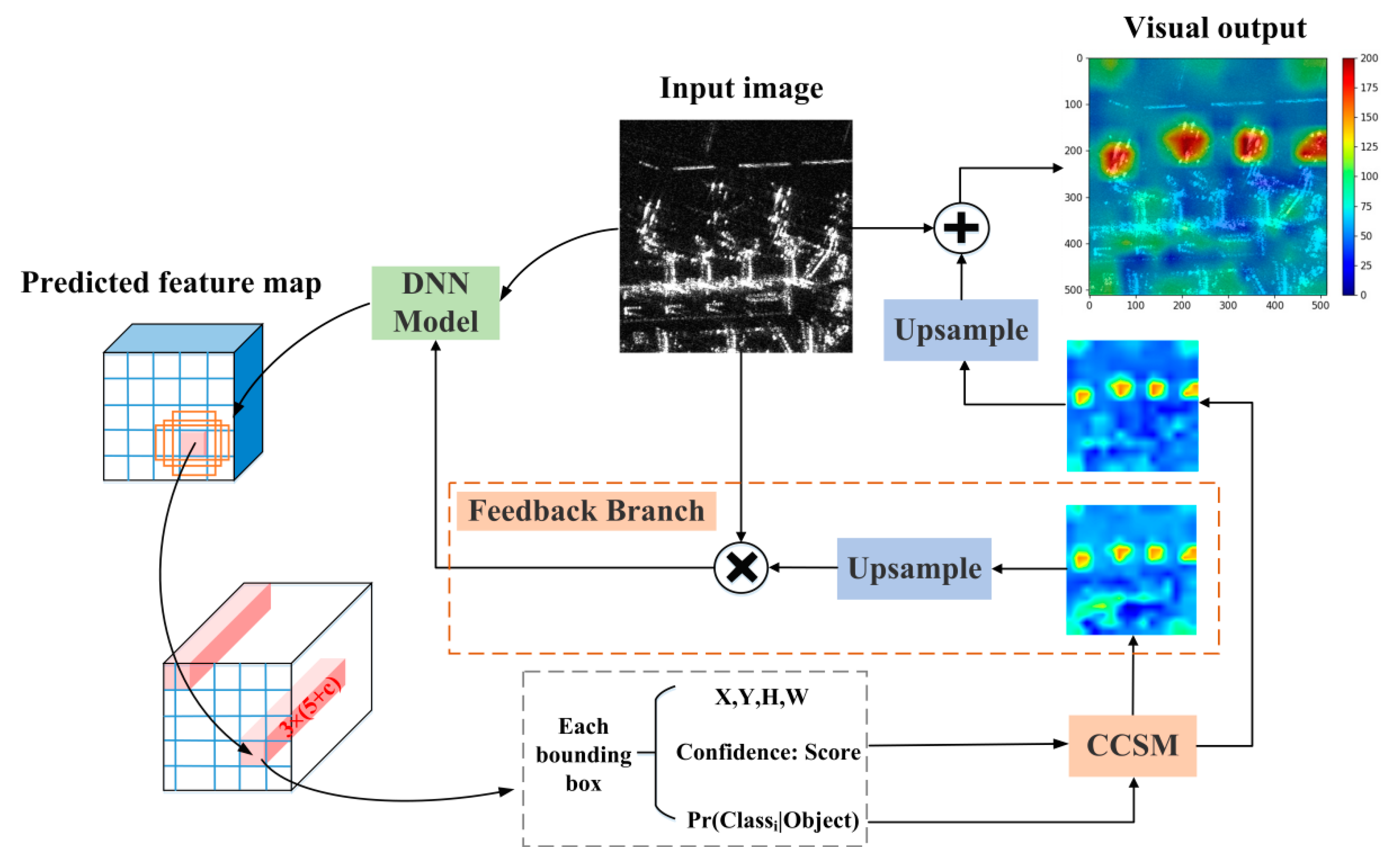
23] for multi-scale detection and then the detection results in the form of marked bounding boxes are produced. In order to understand the detection attributions of the network more comprehensively, the CCSM is proposed in this paper to visualize the predicted feature maps’ output by the detection head to help us understand the detection attribution of the network.
3.2. Hybrid Global Attribution Mapping for the Explanation of Backbone Networks
Selecting a backbone network with a strong feature extraction ability plays an important role in the fields of target detection and classification. At present, most mainstream networks usually adopt the stacking method of feature extraction blocks and down-sampling modules to extract target features, which can be divided into five stages [
24] (as shown in
Figure 1). The effective integration of semantic information and spatial details of feature maps from different levels is conducive to improve the detection accuracy of the network [
25]. Therefore, in this paper, the output feature maps from the last three stages of the backbone network are selected for explanation analysis.
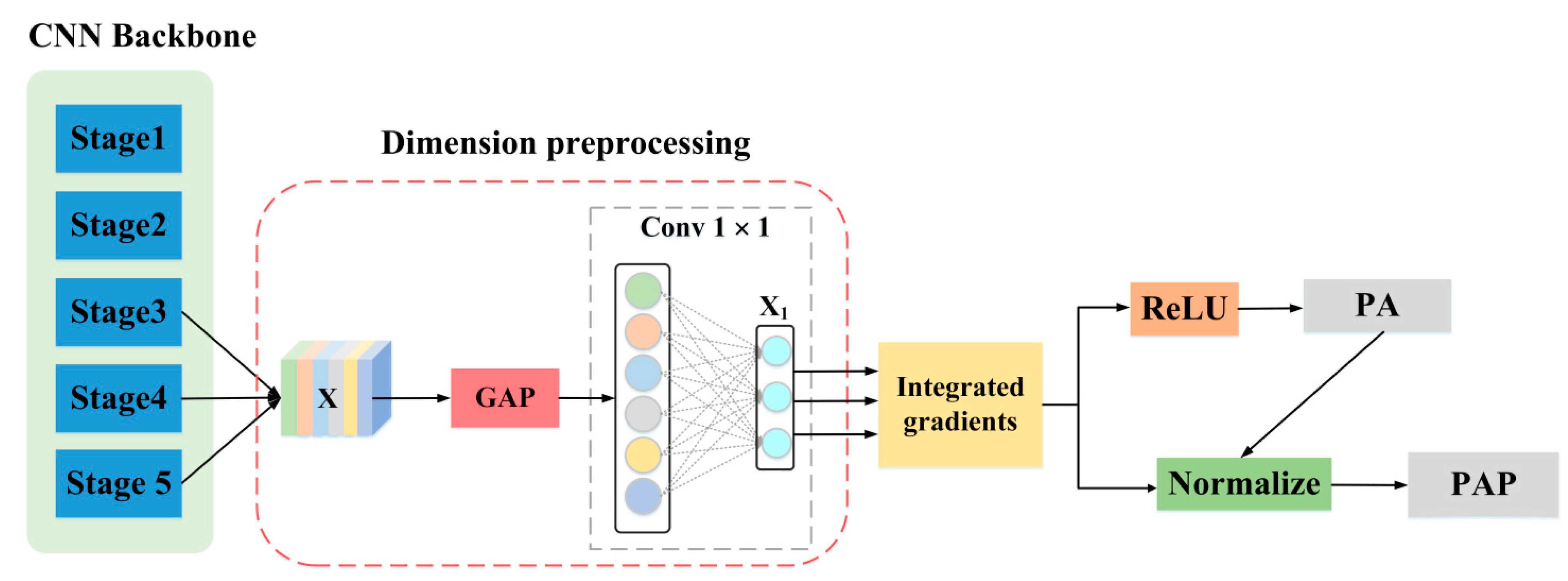
3.2.1. Integrated Gradients
Figure 2 depicts the backbone network based on IG in diagrammatic form. The feature maps output by the backbone network can be represented by a 3-dimensional tensor
. The global average pooling (GAP) can effectively preserve spatial information and object location information while reducing the number of parameters and floating point of operations (FLOPs) of the network [
26,
27]. Therefore, the GAP is used to compress the spatial dimension of feature maps output from the backbone network. Then, a 1 × 1 convolution (the number of convolution kernels are 3 × (5 + C)), and reshape operation are utilized to produce the two-dimensional vector
with size of 3 × (5 + C), where C represents the number of categories. Here,
corresponds to the information of three predicted boxes under the 1 × 1 grid of the predicted feature map in the YOLO network, which encodes the position coordinates, object confidence score and conditional category probability score of each prediction box. By taking the maximum category score box as the final detection result of the target, the IG method is used to generate local observation attributions (including positive attributions and negative attributions) to help us understand the importance of each component in the input feature to the final category prediction.
The IG consider the gradient value of each point on the path from the input image
to the baseline image
, which effectively overcomes the gradient saturation problem of the naive gradient method [
28]. To calculate the total cost
of moving from
to
, the calculation formula of IG is as follows:
where
, which is a parameter curve connecting
and
.
and
represent the original image and the baseline image respectively.
indicates the importance of the
i-th component of input feature
.
A black image (e.g., all pixel values are zero) with the same size as the input image is selected as the baseline in this paper to obtain the local observation attributions output by the network. Then, the positive attribution (PA) and the positive attribution proportion (PAP) of the feature map in the last three stages of the backbone network are calculated, as shown in Equations (2) and (3). Combining the values of PA and PAP, the detection performance analysis of the network on the input samples can be obtained.
where the
is a 3-dimensional tensor with the same shape as the input feature map, which represents the local observation attributions output by the network. The
indicates the ReLU activation function, which is utilized to screen positive attribution. The
and
are the functions of caculating maximum and minimum value, respectively.
3.2.2. Global Attribution Mapping (GAM) for Global Analysis
After obtaining the mean value of PA and PAP of a single input sample in the last three stages of the backbone network, a reasonable number of testing samples (200 aircraft testing samples are selected in this paper heuristically) are injected into the network. Then, the GAM method is used to analyze the detection performance of each backbone network globally. The three main steps of GAM are as follows:
- (1)
Normalize and rank the input attributions. Since each attribution vector (which consists of the mean value of PA or PAP output by each backbone network) in the attributions represents the importance of the input sample feature in the four networks to the final prediction. Thus, the attributions are conjoined rankings. Furthermore, in order to eliminate the impact of size differences in the original input samples, the attributions are normalized into the normalized percentage, as shown in Equation (4).
where
indicates weighted attribution vector, and
represents the weights of feature
i in attribution vector
.
is the Hadamard product.
- (2)
Group similar normalized attributions. Inspired by the idea of clustering, similar attribution data are grouped to obtain the most concentrated feature importance vector to form K clusters. K is a hyperparameter. The value of K indicates the number of interpretative clusters obtained, which can be adjusted to control the interpretation fineness of global attribution. In grouping, it is necessary to measure the similarity between local attributions. Based on the consideration of time complexity, the weighted Spearman’s rho squared rank distance [
29,
30] is selected, as shown in Equation (5). Then, K-Medoids [
31] and weighted Spearman’s rho squared rank distances are combined to group similar attributions. Specifically, the initial center of the K clusters is randomly selected. Then, each input attribution is grouped into the nearest cluster, and then the cluster center is updated by minimizing the pairwise similarity attribution value in the cluster, and iterations are repeated to achieve similarity attribution grouping.
where
and
represent two normalized attribution vectors.
and
represent the ranking of feature
i in the attribution vectors
and
, respectively.
and
indicate the weights of feature
i in corresponding ranking
and
.
- (3)
Generate global attributions. The global explanation is obtained by weighted joint ranking of the importance of attribution features. After grouping similar normalized attributions, K clusters are obtained as the GAM’s global explanation. Each GAM’s global explanation produces a feature importance vector that is most centrally located in the cluster. Moreover, the explanatory power of each global explanation can be measured based on the size of corresponding clusters. By contrast with other clustering methods such as k-means, GAM considers the attribution values encoded in both the rank and weights (named weighted joint ranking) during clustering, which is a unique advantage of GAM.
3.3. Path Aggregation Network (PANet)
After selecting a specific backbone for aircraft feature extraction, the PANet fusion module is used to systematically fuse the semantic features and spatial details from the last three stages of the backbone to enrich the feature expression. As shown in
Figure 1, PANet contains two branches. In one branch, the rich semantic information carried by high-level feature maps are gradually injected into low-level feature maps, in order to improve the discrimination between foreground and background. In the other branch, the low-level feature map that contains a large number of spatial details conducive to target localization, is gradually transmitted to the high-level feature map. After the feature enhancement by the PANet module, three prediction feature maps (P
1, P
2 and P
3) with different resolutions are input into the detection layer for multi-scale prediction, so as to improve the network’s ability to capture targets with different scales.
3.4. Class-Specific Confidence Scores Mapping (CCSM)
Our proposed XAI framework adopts the YOLOv3 head for multi-scale object detection. The whole detection process is shown in
Figure 3. After the input testing image passes through the trained model, three prediction feature maps with different scales are obtained for multi-scale prediction. For each predicted feature map, the information of three groups of bounding boxes generated under each 1 × 1 grid is encoded into a corresponding vector of 3 × (5 + C) (marked in pink in
Figure 3). Each bounding box contains 1 confidence score, four coordinates (center (X, Y), width (W) and height (H)), and C values of conditional category probability
output by the network. The product of conditional category probability and the confidence score of each bounding box is called the category-specific confidence score (CCS), which can better delineate the accuracy of object category information and positioning coordinates [
32].
In the field of classification, CAM (class activation mapping) [
26] enables visualization of specific predicted category scores on the input image, highlighting discriminative parts of objects learned by DNN. In order to more intuitively understand the detection results of the network, the CCSM method is proposed in this paper to visualize the CCS value output by the detection head to understand the final detection attribution of the network. Inspired by Score-CAM [
33], the heat map of CCSM is up-sampled to the size of the input image and multiplied by the original input image to obtain the masked image, which forms a feedback branch. At this time, the masked image mainly retains the key information in the obtained heatmap, and filters out the interference of redundant background information in the original image. Then, it is input into the network again for prediction, and an enhanced heatmap is obtained through secondary correction. The detailed implementation steps of the CCSM module are as follows:
- (1)
Specifying categories and confidence scores for visualization. For each grid of every predicted feature map, the information of three bounding boxes is generated. Therefore, it is necessary to take the maximum category score and the maximum confidence score for the prediction boxes generated under a single feature map as the final visualization score.
- (2)
Normalization. After obtaining the maximum and specified on each feature map, they are normalized to the same range with Equations (6) and (7), which is conducive to the superposition display of the subsequent heatmaps generated on three independent feature maps with different sizes.
where
and
represent the category score and confidence score carried in all bounding boxes generated by the detection network on three prediction feature maps with different sizes, respectively.
- (3)
Generating the heatmap for a single prediction feature map. The product of and is taken as the visualization factor and normalized to generate the heatmap.
- (4)
Visualizing key areas in the final detection result. After obtaining the heatmaps generated on the three prediction feature maps, the heatmaps are up-sampled to the size of the original input image. The outputs can be used in two ways: firstly, the heatmaps can be combined with the original input image in turn to visualize the prediction results layer by layer. Secondly, the three heatmaps (corresponding to the predicted feature maps at three different scales) are integrated with the original input image to visualize the final output of the network.
4. Results
4.1. Experimental Data
The experimental environment is: Unbuntu18.04, Pytorch 1.5, Python 3.8 and a single NVIDIA RTX 2080Ti GPU with 11.00 GB memory. The experimental data adopt 15 large-scale SAR images including different airports with 1 m resolution from the Gaofen-3 system. After the aircraft are manually marked and confirmed by SAR experts, these SAR images are automatically sliced to 512 × 512 pixel samples [
34]. A total of 899 samples were obtained, and then 200 samples were randomly reserved for independent testing sets. For the remaining samples, we combined the methods of rotation, translation (in width and height directions), flipping and mirror to enhance the data, and 3495 aircraft data samples were achieved. The ratio of training set to validation set was 4:1.
4.2. Evaluation Metrics
- (1)
Evaluation Metrics for Backbone Network
Two effective indicators to comprehensively evaluate the performance of the backbone network are used in this paper: global positive attribution (GPA) and global positive attribution proportion (GPAP).
The larger the PA value on a single sample, the stronger the ability of target feature extraction of the network. However, the large positive attribution cannot express the quality of network prediction. Therefore, PAP is further proposed to measure the robustness of network to extract target features. The calculation formulas of PA and PAP can be seen in Equations (2) and (3) in
Section 3.2.1. GPA and GPAP are global indicators evaluated by combining the global information of PA and PAP based on multiple samples. The specific calculation formula is as follows:
where K represents the number of clusters divided by the GAM method, and N is the total number of samples.
denotes the number of samples in the
i-th cluster.
and
are the ranking values of PA and PAP in the
i-th cluster, respectively.
- (2)
Evaluation Metrics for Detection Head
Two evaluation indicators are utilized in this paper: overall box average response (OBAR) and relative discrimination (RD). The OBAR is used to evaluate the average responsiveness of the network to the target area. The RD is used to measure the relative responsiveness of the network to focus on important target areas.
where N represents the number of aircraft labeled boxes on the input image, and BAR (box averages response) denotes the average response value in each labeled box. GAR is the global average response over the entire heatmap.
4.3. Backbone Network Selection Experiment
The backbone network with super characteristic expression ability is a significant cornerstone to maintaining the target detection performance. Meanwhile, the complexity and efficiency of the network are also important considerations. A lightweight network with small parameters is conducive to engineering deployment to solve practical problems, and we have therefore compared three lightweight networks and one network with moderate parameters: ShuffleNetv2 (ShuffleNetv2 × 1.0 Version) [
35], MobileNetv3 (MobileNet v3-small × 1.0 Version) [
24], YOLOv5s (YOLOv5-small Version) [
36] and the classical ResNet-50 [
37].
4.3.1. Contribution Analysis of Single Sample Based on IG Method
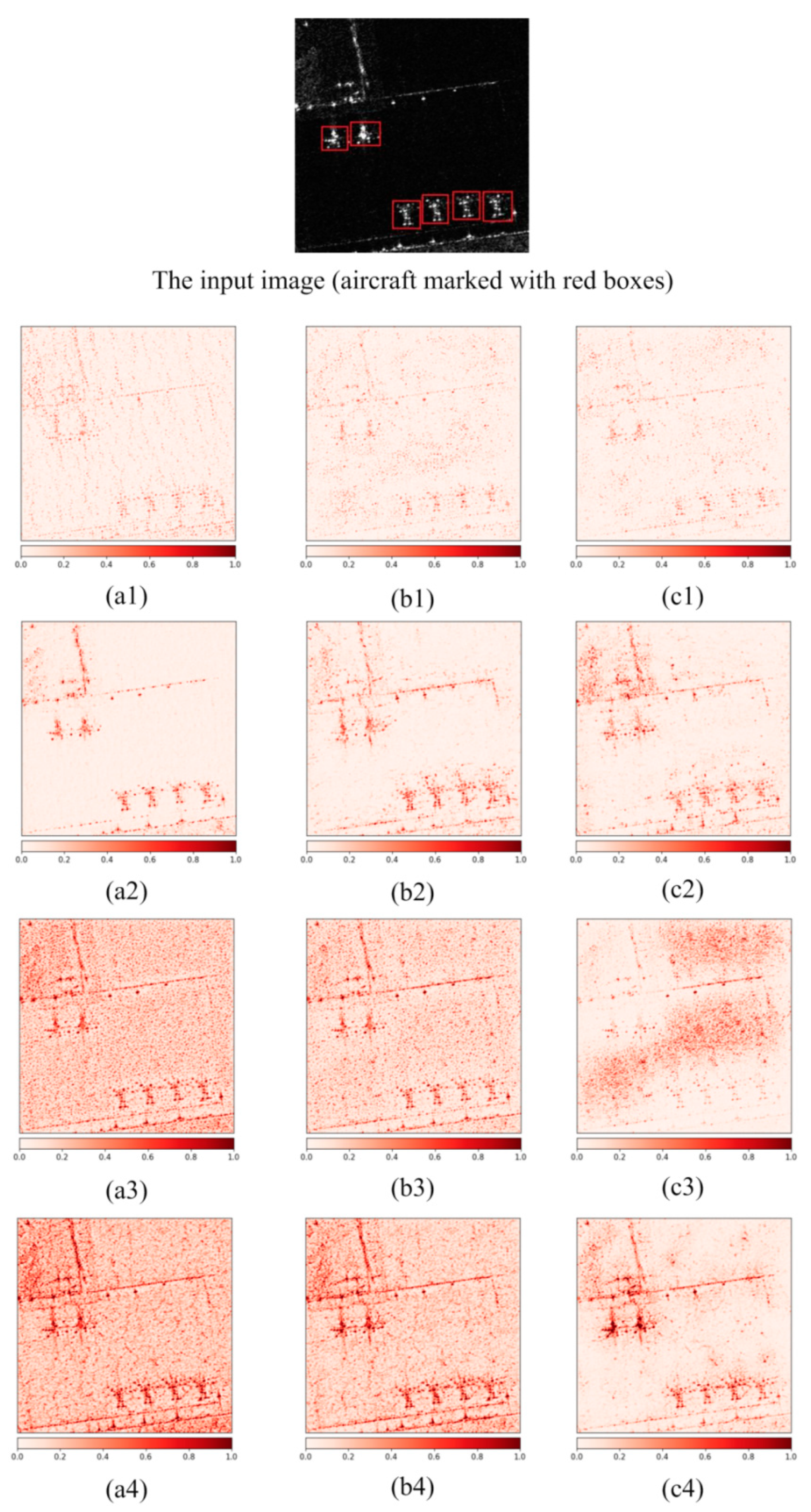
Figure 4 shows the absolute attributions visualization results of four backbone networks in stage 3, stage 4 and stage 5. In the input single sample containing aircraft the attributions are calculated by IG. The attribution value of ShuffleNet v2 (shown in
Figure 4(a1–c1)) in the three stages is low, and the visual significance of an aircraft’s features is poor, which show that the feature extraction ability of ShuffleNet v2 network is weak. In contrast, the aircraft in the absolute attribution figure of MobileNet v3 (shown in
Figure 4(a2–c2)) have a clearer and better visual effect than that of ShuffleNet v2. For ResNet-50, the overall aircraft information can still be well retained in
Figure 4(a3,b3).
With the increase of network depth, aircraft information is gradually submerged by rich semantic information. In
Figure 4(c3), ResNet-50 has large response values (dark red in the figure) mainly concentrated in the background area, and the proportion of aircraft’s scattering characteristics is relatively low. Therefore, the aircraft scattering characteristic information is submerged, which is not conducive to aircraft detection. For YOLOv5s, the absolute attribution values at stage 3 (shown in
Figure 4(a4)) and stage 4 (shown in
Figure 4(b4)) have achieved high response values (the whole picture was dark red). With the deepening of the network, the semantic information obtained is increasingly abundant, and the influence of background noise is also reduced. In stage 5 (shown in
Figure 4(c4)), the features of aircraft still have large response values (dark red in the figure) and good visual effects. It can be seen from this set of experiments that YOLOv5s has an advantage in the detection performance of the aircraft sample.
4.3.2. Global Analysis of Multiple Samples by GAM Algorithm
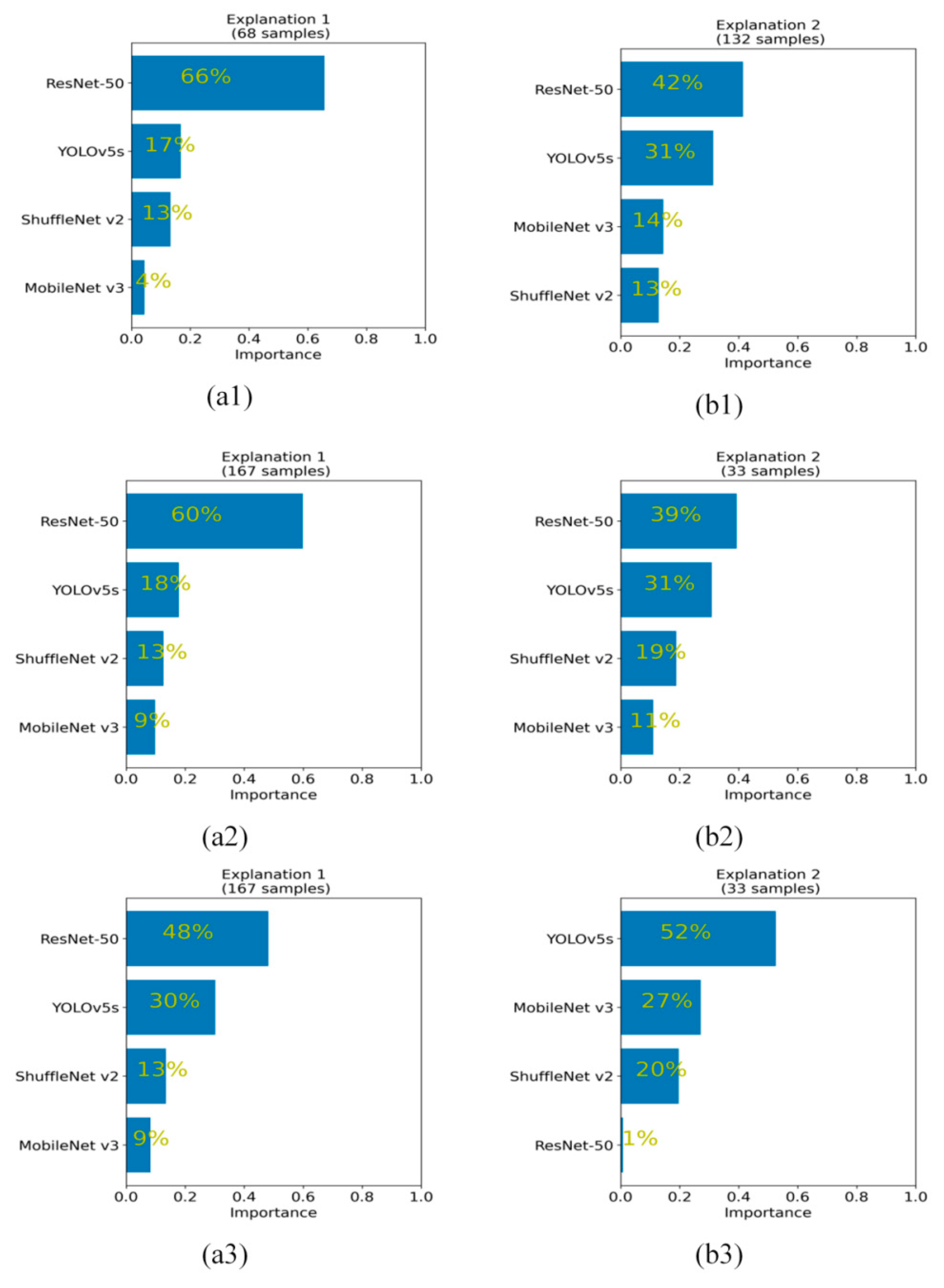
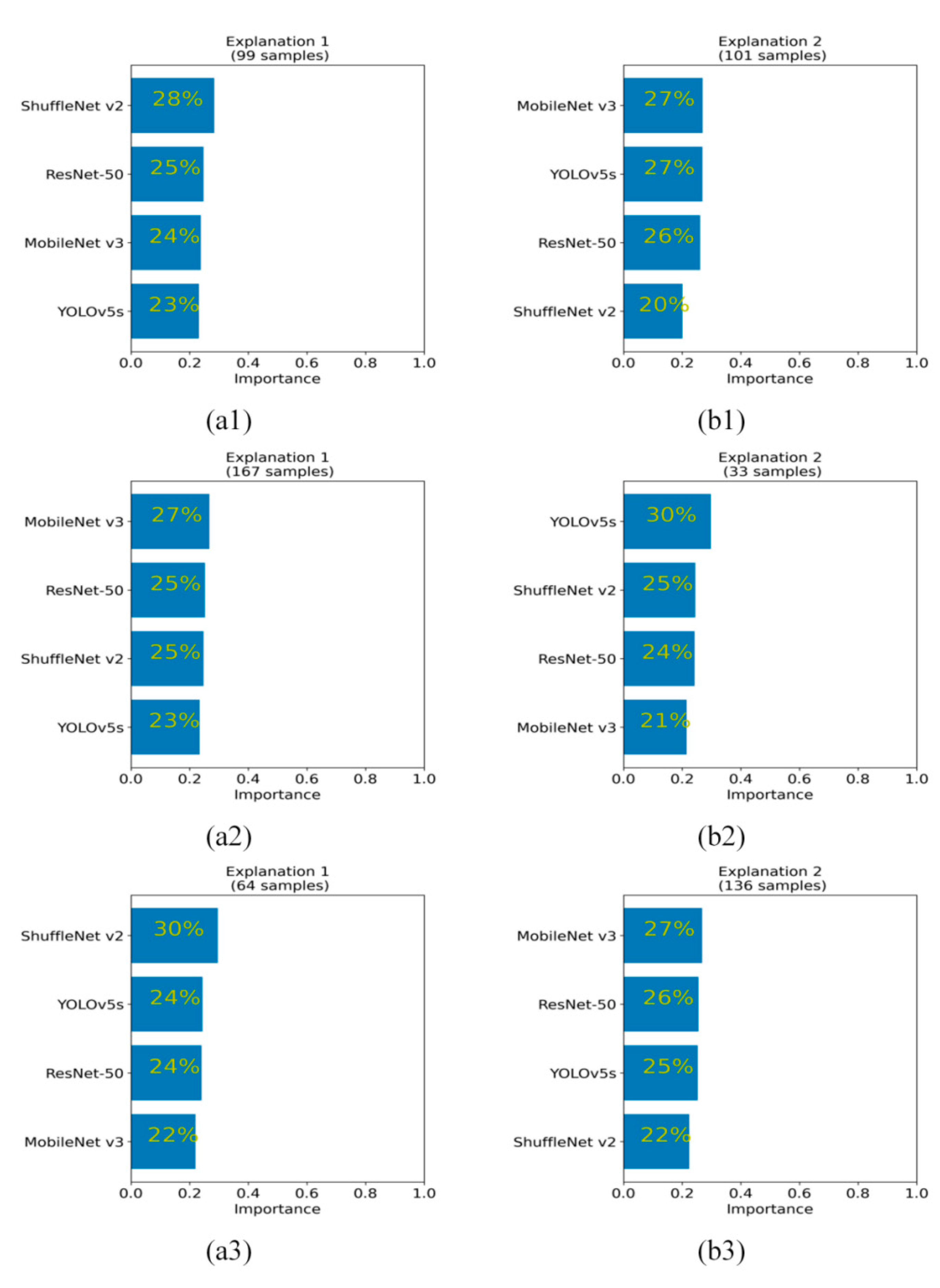
A single sample is not enough to reflect the overall performance evaluation of each network. Therefore, the GAM algorithm is used to evaluate the global performance of each network with 200 independent testing samples (including military aircraft and civil aircraft). In the experiment, K = 2 is selected to generate two clusters.
Figure 5 and
Figure 6 show the global ranking of the average positive attribution and the global ranking of the average positive attribution proportion for the four networks at the last three stages, respectively.
For the global ranking of positive attribution, in stage 3 (shown in
Figure 5(a1,b1)) and stage 4 (shown in
Figure 5(a2,b2)), both ResNet-50 and YOLOv5s have a large global positive attribution ranking, taking first and second place, respectively. ShuffleNet v2 and MobileNet v3 achieved lower rankings. In stage 5 (shown in
Figure 5(a3,b3)), ResNet-50 achieved the highest importance ranking on 167 testing samples (accounting for 83.5% of the total testing samples), as shown in
Figure 5(a3). However, ResNet-50 has the lowest importance among the remaining 33 testing samples (16.5% of the total testing samples), accounting for only 1% of the four network rankings, as shown in
Figure 5(b3). Meanwhile, YOLOv5s achieved the most balanced detection attribution in the two clusters. In cluster 1 (which is composed of 167 testing samples), YOLOv5s accounts for 30%, which follows ResNet-50 in second place. In cluster 2 (which is composed of the remaining 33 test samples), YOLOv5s accounts for 52% and obtains the largest positive attribution advantage. In general, the backbone network of YOLOv5s has the most balanced positive attribution ranking in stages 3, 4 and 5. Therefore, the YOLOv5s network has good feature extraction ability, which is very suitable for the construction of an aircraft detection network.
For the global ranking of positive attribution proportion, whether from the horizontal comparison of two clusters in a single stage or the vertical comparison of each stage, intuitively there is little difference in the global positive attribution proportion of each network, which is shown in
Figure 6.
In order to more intuitively understand the attribution contribution of each stage,
Table 1 shows the index values of the global average positive attribution and the global average positive attribution proportion of the four backbone networks in the last three stages. In terms of global positive attribution (GPA), ResNet-50 is the highest among the four networks. Its average GPA is 48.98. YOLOv5s is the second with the average GPA of 26.67%. The average GPA of MobileNet v3 and ShuffleNet v2 is small, namely, 13.72% and 10.63% respectively. It shows that MobileNet v3 and ShuffleNet v2 have a weak contribution to feature extraction in aircraft detection. In terms of GPAP, there is only a slight difference in the last three stages of the four backbone networks. Among the average GPAP values of each network, the difference between the maximum and minimum values does not exceed 1.2%. In the case of a similar value of GPAP, the larger the GPA, the better the ability of the backbone network to extract effective and robust features of the aircraft. Overall, ResNet-50 obtained the highest value in GPA and GPAP, followed by YOLOv5s. This shows that the backbone networks of ResNet-50 and YOLOv5s can extract more representative and robust aircraft features than MobileNet v3 and ShuffleNet v2.
4.4. Visualization of the Detection Head
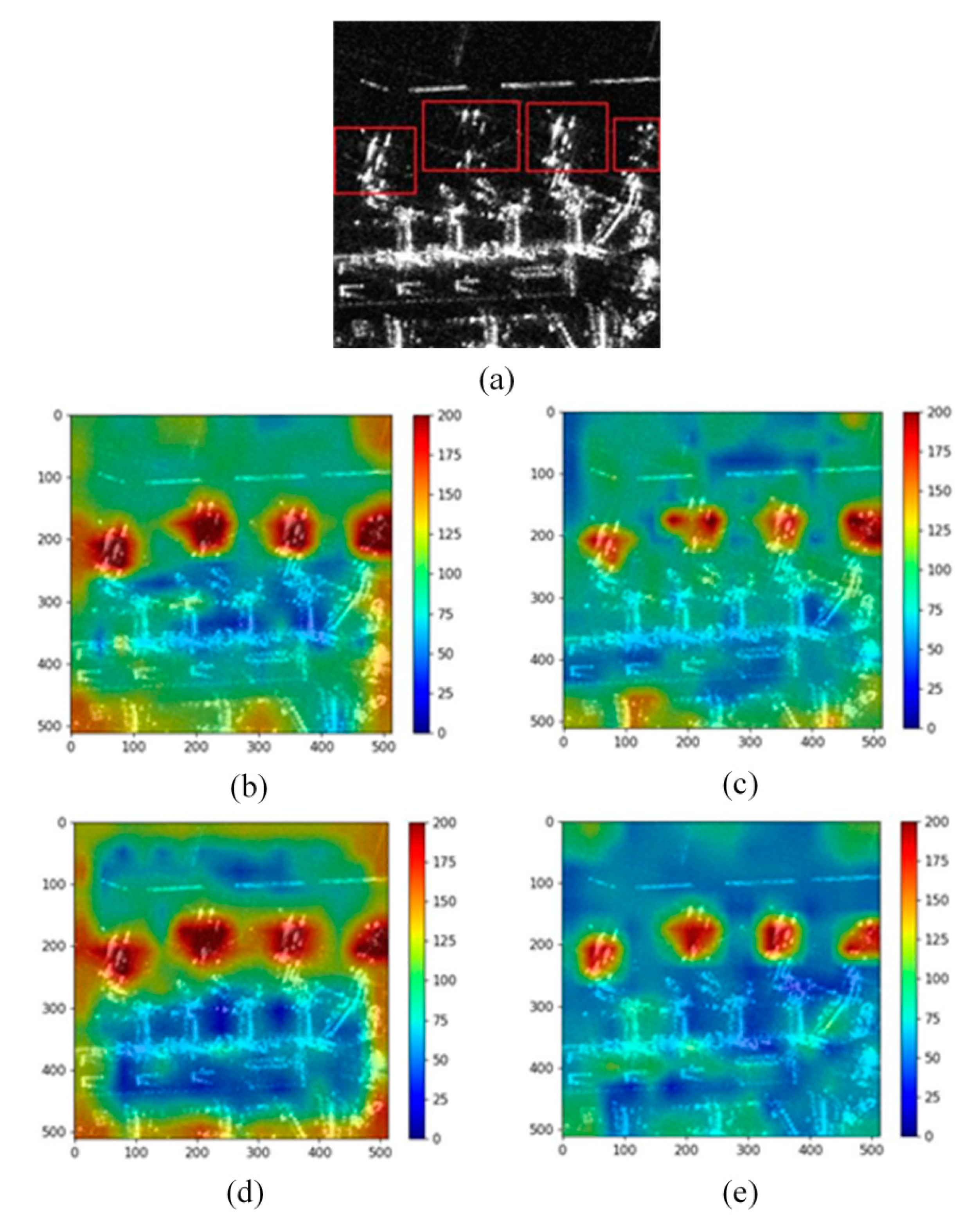
In this paper, the detection results of two different sizes of aircraft, large civil aircraft (Scene I) and small aircraft (Scene II), are visually analyzed, which is more conducive to understanding the detection performance of the network for multi-scale targets.
4.4.1. Scene I
Figure 7 shows the visualized results of the heatmap fused with three branches of the predicted feature map with different sizes.
Figure 7a is part of the scenery of Hongqiao Airport in China. It can be seen that there are four large civil aircraft parked at the airport (marked with red boxes). The features of the aircraft are discrete, and the wing imaging of some aircraft is weak. Due to the relatively obvious overall shape of the fuselage, the heatmaps generated by the four networks can pay more attention to the areas where the aircraft are located. MobileNet v3 (shown in
Figure 7b) and ResNet-50 (shown in
Figure 7d) have high response in the edge region of the image. In contrast, the ShuffleNet v2 (shown in
Figure 7c) and YOLOv5s (shown in
Figure 7e) networks have a good visual effect in the background area, which is mainly distributed in the lower corresponding color areas with pixel values between 50–150. This indicates that the background information has relatively little impact on the final aircraft prediction. It is worth noting that the response of ShuffleNet v2 is relatively scattered, especially on the second aircraft on the left in the figure, which does not perform well on the fuselage or wing.
Table 2 shows the values of relative discrimination and overall box average response, which are used to comprehensively evaluate the network and measure the degree of the focus in important targets areas. ResNet-50 and MobileNet v3 have a higher value of OBAR, but the value of RD is lower than that of ShuffleNet v2 and YOLOv5s. This indicates that the network has high pixel response values in both the aircraft area and background area, so the discrimination of effective aircraft features is relatively weak. Although the OBAR of YOLOv5s is very close to ShuffleNet v2 and lower than ResNet-50 and MobileNet v3, it is worth noting that the YOLOv5s has achieved the highest value of RD of the four backbone networks, which shows that YOLOv5s has a good discrimination between the aircraft and the background.
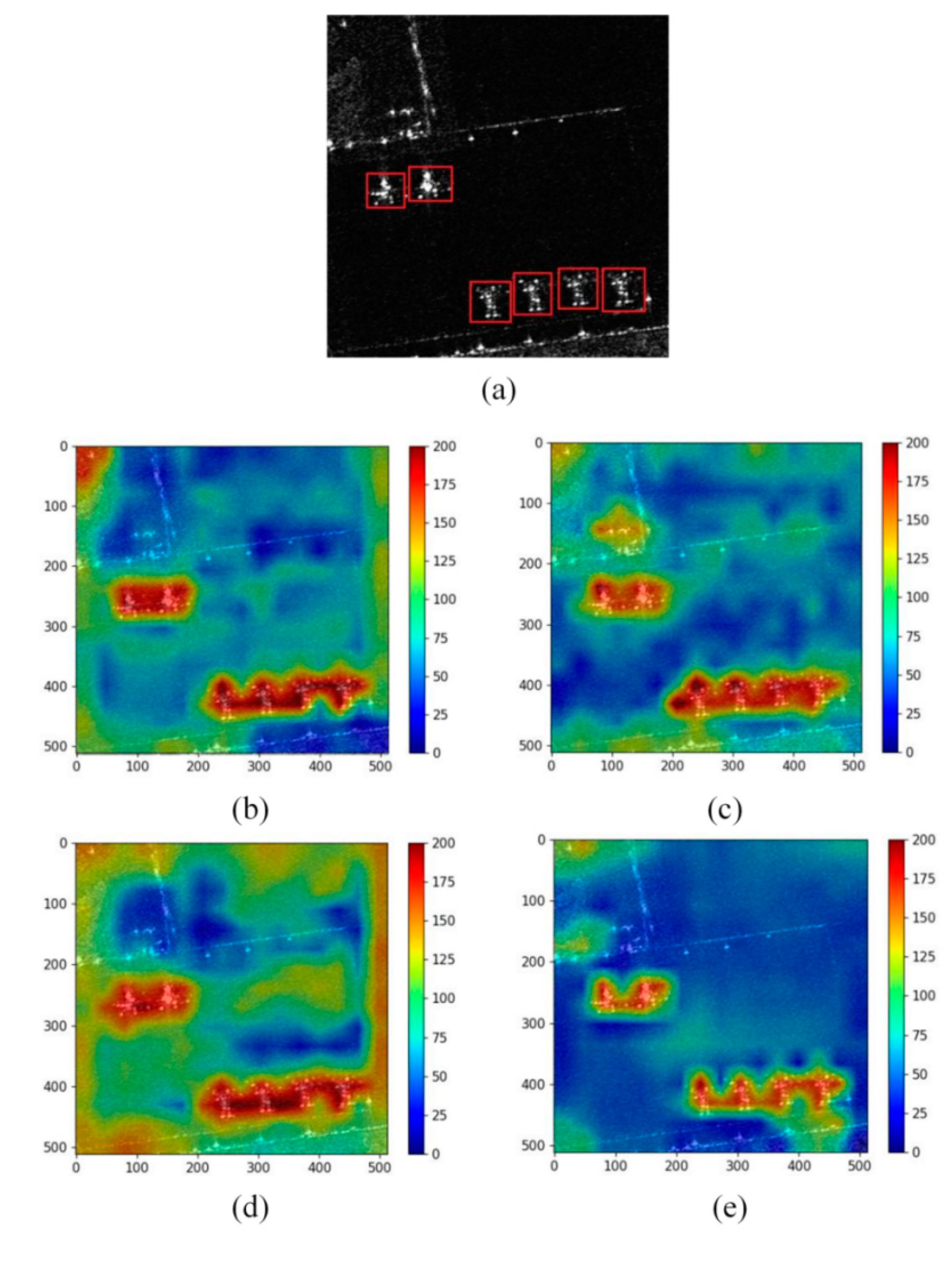
4.4.2. Scene II
Figure 8 shows the local input image from the Capital Airport in China (the aircraft are marked with red boxes) and the output heatmaps of the four backbone networks. The size of the aircraft here is much smaller than that in Scene 1, but the scattering characteristics of the aircraft are obvious. It can be seen from
Figure 8b–e that the four networks can effectively capture the aircrafts’ characteristics. YOLOv5s (as shown in
Figure 8e) has the best visual effect and includes less background noise than the other three networks. At the same time, YOLOv5s has high pixel response values in the fuselage of the aircraft, and the overall aggregation is good. This demonstrates that the YOLOv5s network exhibits superior ability to focus on important characteristics of aircraft in this sample, and has good anti-interference ability. There are some significant effects of background clutter in ShuffleNet v2 (as shown in
Figure 8c) and MobileNet v3 (as shown in
Figure 8b). In particular, the background area response value of ResNet-50 network (as shown in
Figure 8d) is the largest among the four networks, which reflects that ResNet-50 is more likely to suffer from the problem of false detection due to the high impact of background information in the final prediction result.
Table 3 shows the performance analysis of visualization heatmap from the four backbone networks. All the four networks have achieved a large OBAR value. For RD, YOLOv5s has a significant advantage over ShuffleNet v2, MobileNet v3 and ResNet-50 with an RD value of 14.24. Among them, the RD of ResNet-50 network is the lowest, with a value of 10.21, which again shows that the influence of background clutter is great, and the robustness of the ResNet-50 network needs to be further strengthened to obtain better aircraft detection performance.
4.5. Detection Performance of Network Based on Common Metrics
In order to more objectively understand the detection performance of each backbone network,
Table 4 shows the indices comparison of precision, recall and mAP (mean average precision) [
38]. In the whole experiment, the principle of controlling a single variable is adopted, and only the selection of backbone network is different. The same PANet fusion module, YOLOv3 head, and hyperparameter settings are used in the four backbone networks. All networks are trained on the same dataset, and recorded the metrics on the testing set. It can be seen that the results of YOLOv5s and ResNet-50 in recall and mAP are very similar, but the precision of YOLOv5s is 2.38% higher than ResNet-50. This shows that the robustness of the YOLOv5s network is better than that of ResNet-50. MobileNet v3 is ranked third, with precision, recall and map of 86.82%, 92.14% and 90.33%, respectively. ShuffleNet v2 has the lowest value of precision, recall and mAP among the four networks, of which its mAP is 88.06%. This demonstrates that YOLOv5s and ResNet-50 have better aircraft detection performance than ShuffleNet v2 and MobileNet v3. This is consistent with the conclusion obtained by using the IG and GAM method to select the backbone networks, which verifies the effectiveness and feasibility of the backbone networks’ selection method proposed in this paper.
5. Discussion
Selecting a suitable backbone network has now become as important as optimization techniques (e.g., hyperparameter tuning) to achieve high performance in object detection studies. As the network has become increasingly complex, the black-box behaviours of the network are more prominent, hindering the ability of research scientists to understanding the attribution of the network. In order to enhance the transparency of the detection algorithm, an innovative XAI framework for aircraft detection from SAR images based on YOLO detection is proposed.
Due to the scattered image features of aircraft, the heterogeneity of aircraft sizes, and the interference of complex backgrounds, aircraft detection from SAR images is a very challenging task. Therefore, it is particularly important to select a backbone network with feature extraction, especially for the aircraft. The HGAM is proposed in this paper to select the most suitable backbone network for feature extraction of aircraft from SAR images. According to
Table 1, the GPA and GPAP of ResNet-50 and YOLOv5s networks are much higher than that of ShuffleNet v2 and MobileNet v3 networks, which shows the advantages of ResNet-50 and YOLOv5s networks in the extraction of effective features for aircraft. As can be seen from
Figure 5, the global positive attributions ranking of YOLOv5s in the three stages is relatively stable and ranked high. In particular, in cluster 2 of stage 5 (shown in
Figure 5b3), YOLOv5s achieved the highest attributions ranking value of 52% with a great advantage, while ResNet-50 accounts for only 1% of the global positive attribution rankings. This means that on some samples, the output capability and reliability of the top-level module (Stage 5) of ResNet-50 is weaker than that of YOLOv5s. Moreover, combined with the indicators of the CCSM visualization method, as shown in
Table 2 and
Table 3, YOLOv5s has good OBAR value, and its RD is the highest among the four networks. This also shows that background information of YOLOv5s has a minimum impact on the final prediction results, and YOLOv5s can extract aircraft features with good robustness, which has advantages in SAR aircraft detection. This is also verified in
Table 4.
YOLOv5s not only has the highest precision, but it is also very close to ResNet-50 in terms of mAP and recall, and is significantly better than ShuffleNet v2 and MobileNet v3. Therefore, the method proposed in this paper can provide a reliable explanation and analysis of the effectiveness of feature extraction of a given input dataset, and select the appropriate backbone network, which can provide an important reference for other scholars to explain DNN in SAR image analytics.
Furthermore, the XAI framework proposed in this paper is only evaluated for aircraft detection from SAR images (Gaofen-3 images with 1 m resolution). In our future work, we plan to extend our study to multi-scale SAR imagery, and examine more DNNs using HGAM for the selection of the backbone network. At the same time, the explanation of two-stage object detection algorithms (e.g., Faster R-CNN [
39]) will be investigated using the proposed XAI framework, in which we need additional coordination work for the explanation of object localization and recognition. We plan to design a unified XAI approach for object detection to promote the understandability and application of DNN in SAR image analytics.
6. Conclusions
In this paper, an innovative XAI framework has been proposed by combining the HGAM algorithm, PANet, and the metrics of CCSM, to glassbox DNN with high performance and understandability. This framework offers explanation information for the determination of backbone networks in object detection from SAR imagery, and provides visualization of the discriminatory power of detection heads. To the best of our knowledge, this is the first XAI paper in SAR-based object detection studies, and it paves the path for future exploration of XAI to enhance the comprehensibility, transparency, traceability, causality and trust in the employment of DNN.
Author Contributions
Methodology, R.L., J.X., and L.C.; software, R.L. and X.C.; validation, Z.L., R.L. and X.C.; formal analysis, R.L.; investigation, J.X., L.C., X.C.; data curation, J.W., Z.P. and Z.L.; writing—original draft preparation, R.L. and J.X.; writing—review and editing, L.C., A.F., and J.X.; visualization, R.L.; supervision, Z.P.; project administration, X.C., Z.P. and J.W.; funding acquisition, L.C. All authors contributed extensively to this manuscript. All authors have read and agreed to the published version of the manuscript.
Funding
This research was supported by National Natural Science Foundation of China, grant number 42101468 and 61701047, partly funded by the Foundation of Hunan, Education Committee, under Grants No. 20B038.
Institutional Review Board Statement
Not applicable.
Informed Consent Statement
Not applicable.
Data Availability Statement
The data are Gaofen-3 system data with 1m resolution provided by a third party, not a public dataset. The data are not made public due to copyright issues.
Acknowledgments
We also sincerely thank the anonymous reviewers for their critical comments and suggestions for improving the manuscript.
Conflicts of Interest
The authors declare no conflict of interest.
References
- El-Darymli, K.; Gill, E.W.; Mcguire, P.; Power, D.; Moloney, C. Automatic target recognition in synthetic aperture radar im-agery: A state-of-the-art review. IEEE Access 2016, 4, 6014–6058. [Google Scholar] [CrossRef] [Green Version]
- Wang, J.; Xiao, H.; Chen, L.; Xing, J.; Pan, Z.; Luo, R.; Cai, X. Integrating weighted feature fusion and the spatial attention module with convolutional neural networks for automatic aircraft detection from SAR images. Remote Sens. 2021, 13, 910. [Google Scholar] [CrossRef]
- Luo, R.; Chen, L.; Xing, J.; Yuan, Z.; Tan, S.; Cai, X.; Wang, J. A fast aircraft detection method for SAR images based on efficient bidirectional path aggregated attention network. Remote Sens. 2021, 13, 2940. [Google Scholar] [CrossRef]
- Thiagarajan, J.J.; Ramamurthy, K.N.; Knee, P.; Spanias, A.; Berisha, V. Sparse representations for automatic target classification in SAR images. In Proceedings of the 2010 4th International Symposium on Communications, Control and Signal Processing (ISCCSP), Limassol, Cyprus, 3–5 March 2010; pp. 1–4. [Google Scholar]
- Zhu, X.X.; Tuia, D.; Mou, L.; Xia, G.-S.; Zhang, L.; Xu, F.; Fraundorfer, F. Deep learning in remote sensing: A comprehensive review and list of resources. IEEE Geosci. Remote Sens. Mag. 2017, 5, 8–36. [Google Scholar] [CrossRef] [Green Version]
- Zhu, X.; Montazeri, S.; Ali, M.; Hua, Y.; Wang, Y.; Mou, L.; Shi, Y.; Xu, F.; Bamler, R. Deep learning meets SAR: Concepts, models, pitfalls, and perspectives. IEEE Geosci. Remote Sens. Mag. 2021. [Google Scholar] [CrossRef]
- Tan, Y.; Li, Q.; Li, Y.; Tian, J. Aircraft detection in high-resolution SAR images based on a gradient textural saliency map. Sensors 2015, 15, 23071–23094. [Google Scholar] [CrossRef] [PubMed]
- Tan, S.; Chen, L.; Pan, Z.; Xing, J.; Li, Z.; Yuan, Z. Geospatial contextual attention mechanism for automatic and fast airport detection in SAR imagery. IEEE Access 2020, 8, 173627–173640. [Google Scholar] [CrossRef]
- Ren, H.; Yu, X.; Zou, L.; Zhou, Y.; Wang, X.; Bruzzone, L. Extended convolutional capsule network with application on SAR automatic target recognition. Signal Process. 2021, 183, 108021. [Google Scholar] [CrossRef]
- Adadi, A.; Berrada, M. Peeking inside the black-box: A survey on explainable artificial intelligence (XAI). IEEE Access 2018, 6, 52138–52160. [Google Scholar] [CrossRef]
- Arrieta, A.B.; Díaz-Rodríguez, N.; Del Ser, J.; Bennetot, A.; Tabik, S.; Barbado, A.; Garcia, S.; Gil-Lopez, S.; Molina, D.; Benjamins, R.; et al. Explainable Artificial Intelligence (XAI): Concepts, taxonomies, opportunities and challenges toward responsible AI. Inf. Fusion 2019, 58, 82–115. [Google Scholar] [CrossRef] [Green Version]
- Holzinger, A.; Carrington, A.; Müller, H. Measuring the quality of explanations: The system causability scale (SCS): Comparing human and machine explanations. KI-Künstliche Intell. 2020, 34, 1–6. [Google Scholar] [CrossRef] [Green Version]
- Mandeep, M.; Pannu, H.S.; Malhi, A. Deep learning-based explainable target classification for synthetic aperture radar images. In Proceedings of the 13th International Conference on Human System Interaction (HSI), Tokyo, Japan, 6–8 June 2020; pp. 34–39. [Google Scholar] [CrossRef]
- Qi, Z.; Khorram, S.; Fuxin, L. Visualizing deep networks by optimizing with integrated gradients. Proc. Conf. AAAI Ar. Int. 2020, 34, 11890–11898. [Google Scholar] [CrossRef]
- Ibrahim, M.; Louie, M.; Modarres, C.; Paisley, J. Global explanations of neural networks: Mapping the landscape of predictions. In Proceedings of the 2019 AAAI/ACM Conference on AI, Ethics, and Society (AIES), Honolulu, HI, USA, 27–28 January 2019; pp. 279–287. [Google Scholar] [CrossRef]
- Guo, X.; Hou, B.; Ren, B.; Ren, Z.; Jiao, L. Network pruning for remote sensing images classification based on interpretable CNNs. IEEE Trans. Geosci. Remote Sens. 2021, 1–15. [Google Scholar] [CrossRef]
- Abdollahi, A.; Pradhan, B. Urban vegetation mapping from aerial imagery using Explainable AI (XAI). Sensors 2021, 21, 4738. [Google Scholar] [CrossRef] [PubMed]
- Lundberg, S.M.; Lee, S.I. A unified approach to interpreting model predictions. In Proceedings of the 31st International Conference on Neural Information Processing Systems, Long Beach, CA, USA, 4 December 2017; pp. 4768–4777. [Google Scholar]
- Matin, S.; Pradhan, B. Earthquake-induced building-damage mapping using Explainable AI (XAI). Sensors 2021, 21, 4489. [Google Scholar] [CrossRef] [PubMed]
- Samek, W.; Montavon, G.; Lapuschkin, S.; Anders, C.J.; Muller, K.-R. Explaining deep neural networks and beyond: A review of methods and applications. Proc. IEEE 2021, 109, 247–278. [Google Scholar] [CrossRef]
- Jin, G.; Taniguchi, R.-I.; Qu, F. Auxiliary detection head for one-stage object detection. IEEE Access 2020, 8, 85740–85749. [Google Scholar] [CrossRef]
- Liu, S.; Qi, L.; Qin, H.; Shi, J.; Jia, J. Path aggregation network for instance segmentation. In Proceedings of the IEEE/CVF Conference on Computer Vision and Pattern Recognition, Salt Lake City, UT, USA, 18–23 June 2018; pp. 8759–8768. [Google Scholar] [CrossRef] [Green Version]
- Redmon, J.; Farhadi, A. YOLOv3: An incremental improvement. arXiv 2018, arXiv:1804.02767v1. [Google Scholar]
- Howard, A.; Sandler, M.; Chen, B.; Wang, W.; Chen, L.-C.; Tan, M.; Chu, G.; Vasudevan, V.; Zhu, Y.; Pang, R.; et al. Searching for MobileNetV3. In Proceedings of the IEEE/CVF International Conference on Computer Vision (ICCV), Seoul, Korea, 27 October–2 November 2019; pp. 1314–1324. [Google Scholar] [CrossRef]
- Lin, T.; Dollár, P.; Girshick, R.; He, K.; Hariharan, B.; Belongie, S. Feature pyramid networks for object detection. In Proceedings of the IEEE Conference on Computer Vision and Pattern Recognition (CVPR), Honolulu, HI, USA, 21–26 July 2017; pp. 936–944. [Google Scholar] [CrossRef] [Green Version]
- Zhou, B.; Khosla, A.; Lapedriza, A.; Oliva, A.; Torralba, A. Learning deep features for discriminative localization. In Proceedings of the IEEE Conference on Computer Vision and Pattern Recognition (CVPR), Las Vegas, NV, USA, 27–30 June 2016; pp. 2921–2929. [Google Scholar] [CrossRef] [Green Version]
- Lin, M.; Chen, Q.; Yan, S. Network in network. arXiv 2013, arXiv:1312.4400v3. [Google Scholar]
- Sundararajan, M.; Taly, A.; Yan, Q. Gradients of counterfactuals. arXiv 2016, arXiv:1611.02639v2. [Google Scholar]
- Lee, P.; Yu, P. Mixtures of weighted distance-based models for ranking data with applications in political studies. Comput. Stat. Data Anal. 2012, 56, 2486–2500. [Google Scholar] [CrossRef]
- Shieh, G.S.; Bai, Z.; Tsai, W.-Y. Rank tests for independence with a weighted contamination alternative. Stat. Sin. 2000, 10, 577–593. [Google Scholar]
- Park, H.-S.; Jun, C.-H. A simple and fast algorithm for K-medoids clustering. Expert Syst. Appl. 2009, 36, 3336–3341. [Google Scholar] [CrossRef]
- Huang, Z.; Wang, J. DC-SPP-YOLO: Dense connection and spatial pyramid pooling based YOLO for object detection. arXiv 2019, arXiv:1903.08589v1. [Google Scholar] [CrossRef] [Green Version]
- Wang, H.; Wang, Z.; Du, M.; Yang, F.; Zhang, Z.; Ding, S.; Mardziel, P.; Hu, X. Score-CAM: Score-weighted visual explanations for convolutional neural networks. In Proceedings of the IEEE/CVF Conference on Computer Vision and Pattern Recognition Workshops (CVPRW), Seattle, WA, USA, 14–19 June 2020; pp. 111–119. [Google Scholar] [CrossRef]
- Xing, J.; Sieber, R.; Kalacska, M. The challenges of image segmentation in big remotely sensed imagery data. Ann. GIS 2014, 20, 233–244. [Google Scholar] [CrossRef]
- Ma, N.; Zhang, X.; Zheng, H.; Sun, J. ShuffleNet V2: Practical guidelines for efficient CNN architecture design. arXiv 2018, arXiv:1807.11164. [Google Scholar]
- Ultralytics. Yolov5. Available online: https://github.com/ultralytics/yolov5 (accessed on 18 May 2020).
- He, K.; Zhang, X.; Ren, S.; Sun, J. Deep residual learning for image recognition. In Proceedings of the IEEE Conference on Computer Vision and Pattern Recognition (CVPR), Las Vegas, NV, USA, 27–30 June 2016; pp. 770–778. [Google Scholar]
- Everingham, M.; Van Gool, L.; Williams, C.K.I.; Winn, J.; Zisserman, A. The pascal visual object classes (VOC) challenge. Int. J. Comput. Vis. 2009, 88, 303–338. [Google Scholar] [CrossRef] [Green Version]
- Ren, S.; Kaiming, H.; Girshick, R.; Sun, J. Faster r-cnn: Towards real-time object detection with region proposal networks. IEEE Trans. Pattern Anal. Mach. Intell. 2017, 39, 1137–1149. [Google Scholar] [CrossRef] [Green Version]
Figure 1.
The overall architecture of the proposed eXplainable Artificial Intelligence (XAI) framework for aircraft detection.
Figure 1.
The overall architecture of the proposed eXplainable Artificial Intelligence (XAI) framework for aircraft detection.
Figure 2.
Backbone network based on IG: the GAP represents global average pooling, ReLU represents rectified linear unit (ReLU) activation function, which is used to screen positive attribution (PA). The obtained gradient attributions and PA are utilized to obtain the positive attribution proportion (PAP).
Figure 3.
Visual diagram of detection process.
Figure 3.
Visual diagram of detection process.
Figure 4.
Visualization results of integral gradient (IG) absolute attribution in stage 3, stage 4 and stage 5 of backbone network. (a1–c1), (a2–c2), (a3–c3) and (a4–c4) represent the IG-based absolute attribution visualization results of ShuffleNet v2, MobileNet v3, ResNet-50 and YOLOv5s at stage 3, stage 4 and stage 5 respectively.
Figure 5.
The global positive attribution analysis based on integral gradient (IG). (a1,b1), (a2,b2), (a3,b3) represent the positive attribution distribution of the four backbone networks in stage 3, stage 4 and stage 5 respectively.
Figure 5.
The global positive attribution analysis based on integral gradient (IG). (a1,b1), (a2,b2), (a3,b3) represent the positive attribution distribution of the four backbone networks in stage 3, stage 4 and stage 5 respectively.
Figure 6.
Analysis of global positive attribution proportion based on IG. (a1,b1), (a2,b2), (a3,b3) respectively represent the global distribution of the positive attribution proportion of the four backbone networks in stage 3, stage 4 and stage 5.
Figure 6.
Analysis of global positive attribution proportion based on IG. (a1,b1), (a2,b2), (a3,b3) respectively represent the global distribution of the positive attribution proportion of the four backbone networks in stage 3, stage 4 and stage 5.
Figure 7.
The visualized result of the heatmap for Scene I. (a) is the ground truth of Scene I from Hongqiao Airport in China, in which the aircraft are marked with red boxes. (b–e) are the heat maps output by MobileNet v3, ShuffleNet v2, ResNet-50, and YOLOv5s, respectively.
Figure 7.
The visualized result of the heatmap for Scene I. (a) is the ground truth of Scene I from Hongqiao Airport in China, in which the aircraft are marked with red boxes. (b–e) are the heat maps output by MobileNet v3, ShuffleNet v2, ResNet-50, and YOLOv5s, respectively.
Figure 8.
The visualized result of the heatmap for Scene II. (a) is the ground truth of Scene II from Capital Airport in China, in which the aircraft are marked with red boxes. (b–e) are the heat maps output by MobileNet v3, ShuffleNet v2, ResNet-50, and YOLOv5s, respectively.
Figure 8.
The visualized result of the heatmap for Scene II. (a) is the ground truth of Scene II from Capital Airport in China, in which the aircraft are marked with red boxes. (b–e) are the heat maps output by MobileNet v3, ShuffleNet v2, ResNet-50, and YOLOv5s, respectively.
Table 1.
Comparison of GPA and GPAP metrics of four networks in the last three stages.
Table 1.
Comparison of GPA and GPAP metrics of four networks in the last three stages.
| Network | Stage | Global Positive Attribution (GPA) (%) | Global Positive Attribution Proportion (GPAP) (%) |
|---|
| ShuffleNet v2 | Stage 3 | 13.00 | 23.96 |
| Stage 4 | 13.99 | 25.00 |
| Stage 5 | 14.16 | 24.56 |
| Mean | 13.72 | 24.51 |
| MobileNet v3 | Stage3 | 10.60 | 25.52 |
| Stage 4 | 9.33 | 26.01 |
| Stage 5 | 11.97 | 25.40 |
| Mean | 10.63 | 25.64 |
| ResNet-50 | Stage 3 | 50.16 | 25.51 |
| Stage 4 | 56.54 | 24.84 |
| Stage 5 | 40.25 | 25.36 |
| Mean | 48.98 | 25.52 |
| YOLOv5s | Stage 3 | 26.24 | 25.02 |
| Stage 4 | 20.15 | 24.16 |
| Stage 5 | 33.63 | 24.68 |
| Mean | 26.67 | 24.62 |
Table 2.
Performance analysis of visual heatmap of four networks.
Table 2.
Performance analysis of visual heatmap of four networks.
| Network | Overall Box Average Response (OBAR) | Relative Discrimination (RD) |
|---|
| ShuffleNet v2 | 127 | 5.98 |
| MobileNet v3 | 155 | 5.66 |
| ResNet-50 | 160 | 5.83 |
| YOLOv5s | 128 | 6.54 |
Table 3.
Performance analysis of visual heatmap of four networks.
Table 3.
Performance analysis of visual heatmap of four networks.
| Network | Overall Box Average Response (OBAR) | Relative Discrimination (RD) |
|---|
| ShuffleNet v2 | 164 | 12.57 |
| MobileNet v3 | 175 | 12.97 |
| ResNet-50 | 174 | 10.21 |
| YOLOv5s | 146 | 14.24 |
Table 4.
Performance comparison of four object detection networks.
Table 4.
Performance comparison of four object detection networks.
| Models | Precision (%) | Recall (%) | mAP (%) |
|---|
ShuffleNet v2
(PANet + YOLOv3 Head) | 83.68 | 90.61 | 88.06 |
MobileNet v3
(PANet + YOLOv3 Head) | 86.82 | 92.14 | 90.33 |
ResNet-50
(PANet + YOLOv3 Head) | 89.25 | 93.60 | 92.02 |
YOLOv5s
(PANet + YOLOv3 Head) | 91.63 | 93.25 | 91.58 |
| Publisher’s Note: MDPI stays neutral with regard to jurisdictional claims in published maps and institutional affiliations. |
© 2021 by the authors. Licensee MDPI, Basel, Switzerland. This article is an open access article distributed under the terms and conditions of the Creative Commons Attribution (CC BY) license (https://creativecommons.org/licenses/by/4.0/).


 ,
, 


