
Automatic Detection of Impervious Surfaces from Remotely Sensed Data Using Deep Learning

 and
and 
Abstract
:1. Introduction
2. Related Work
2.1. Statistical Indices
2.1.1. NDVI
2.1.2. NDBI
2.1.3. NDISI
2.1.4. PISI
2.1.5. Analysis
2.2. Classification and Regression Methods
2.3. Deep Learning Neural Networks
2.4. Gradient Descent Optimization
3. Methodology
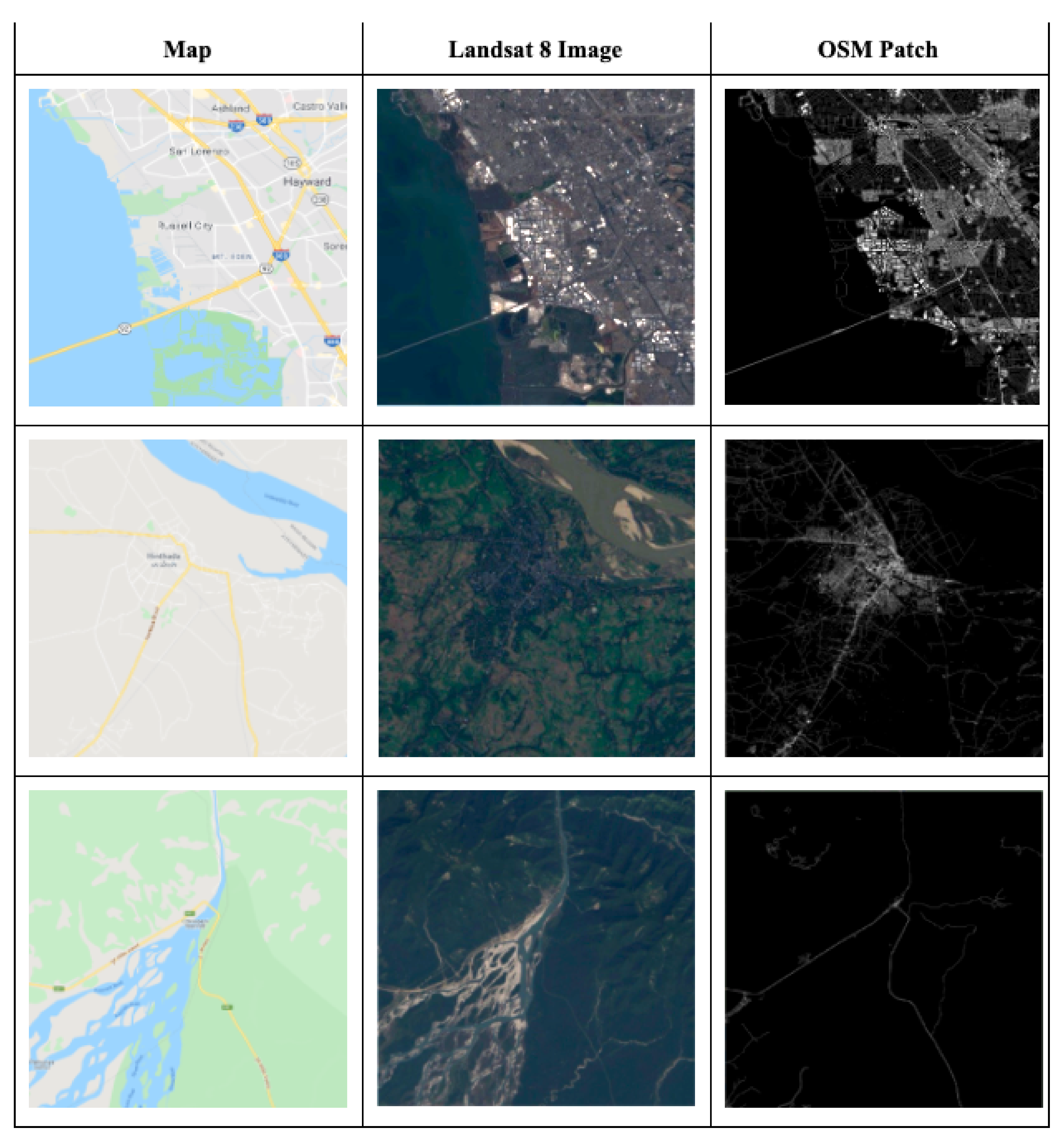
3.1. Input Features
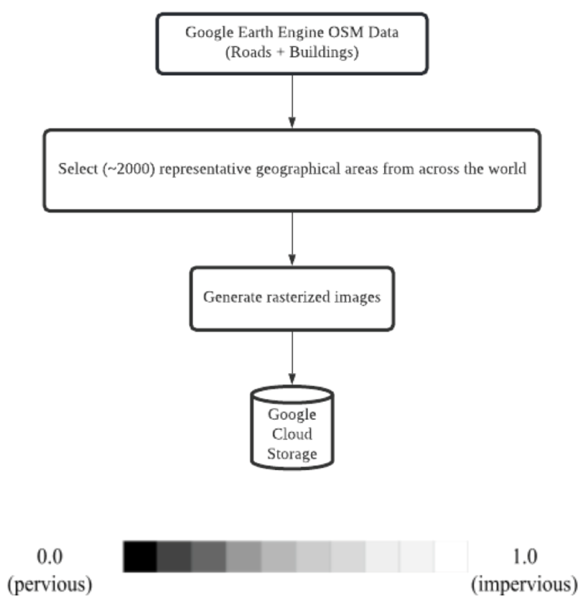
3.2. Impervious Surface Labels
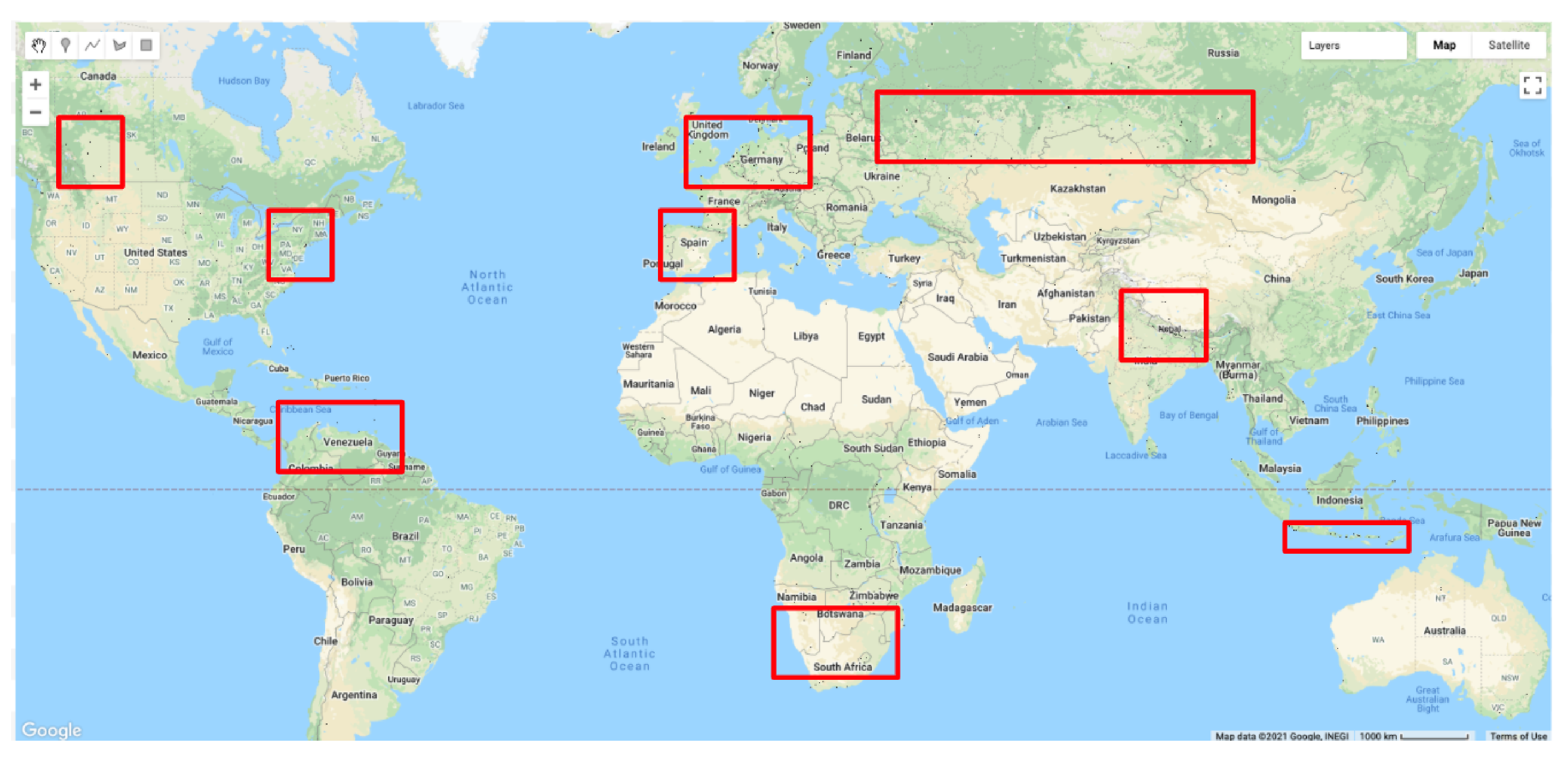
3.3. Dataset Generation
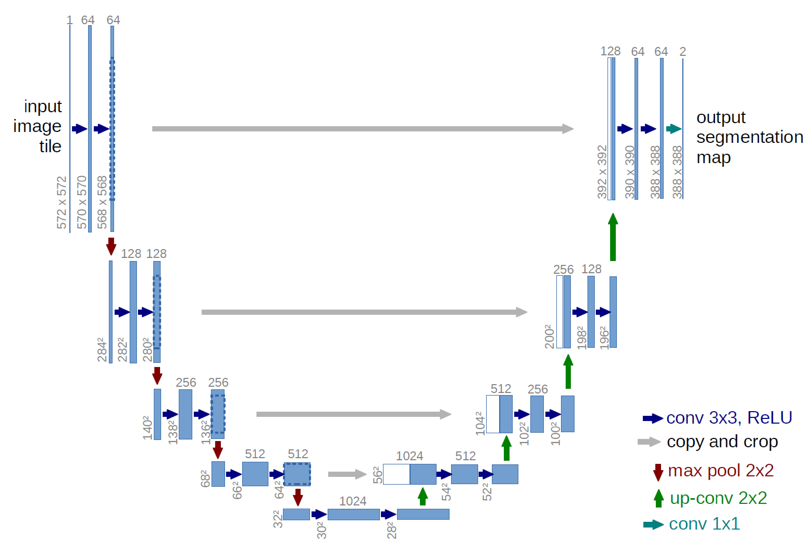
3.4. Models
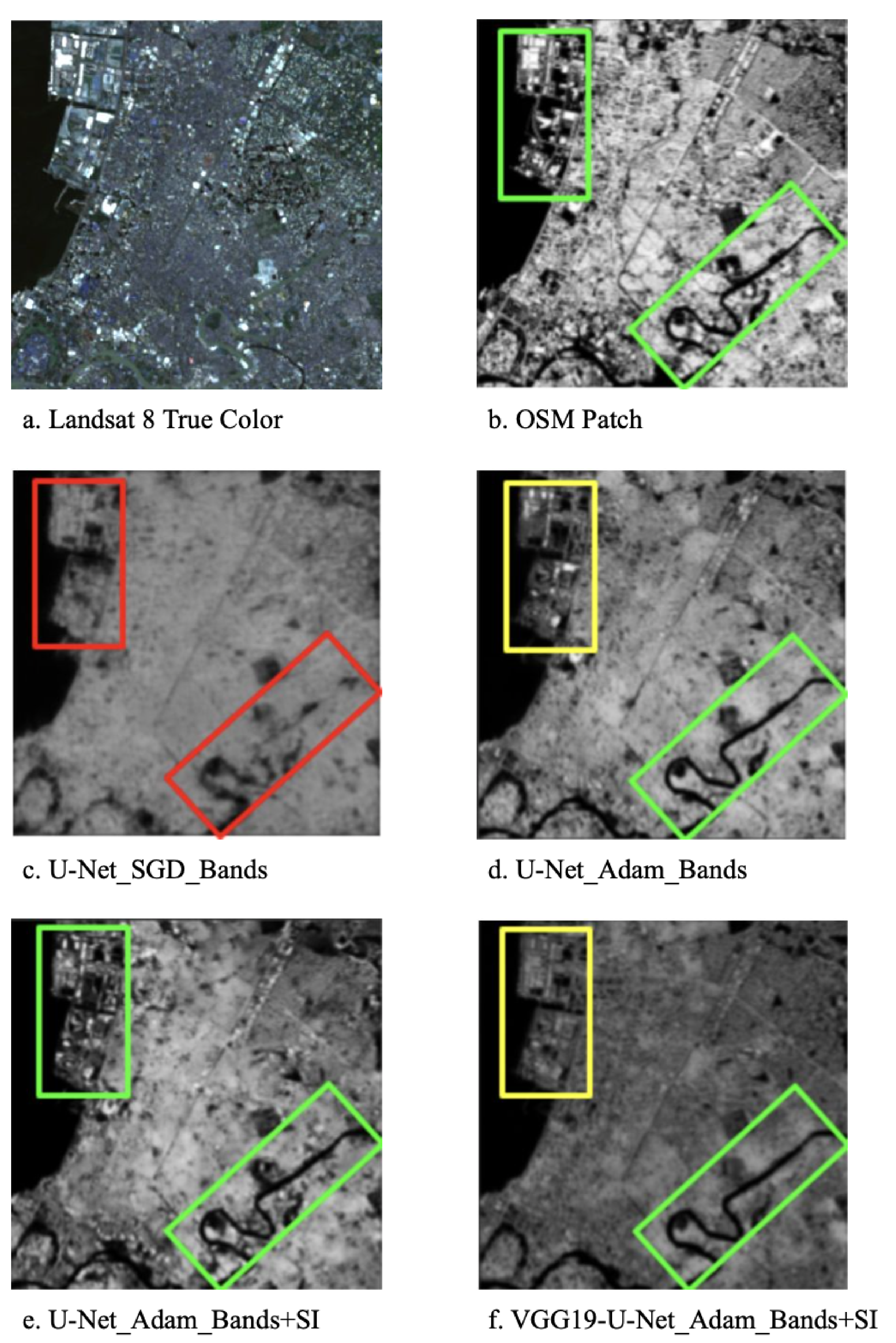
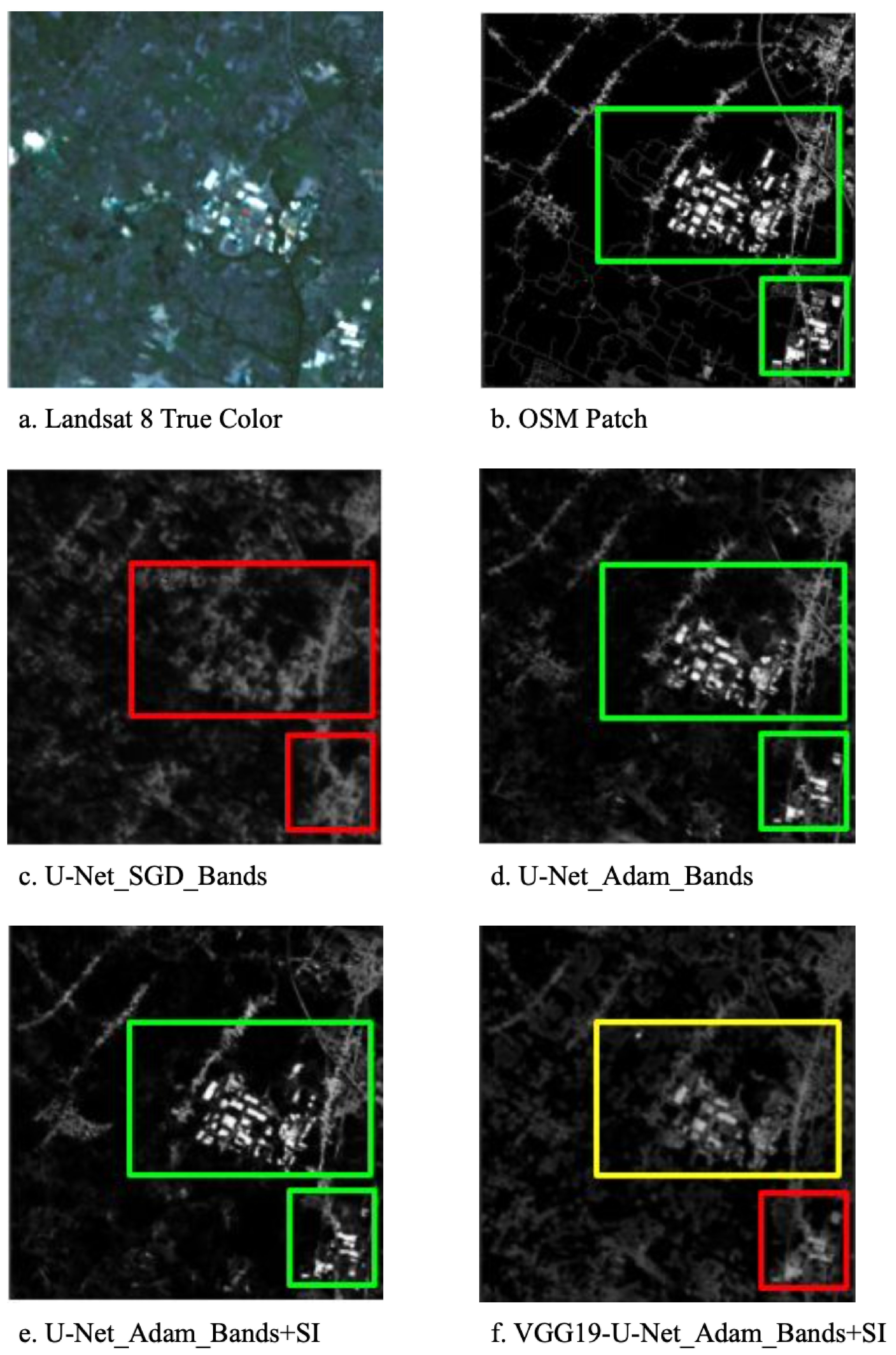
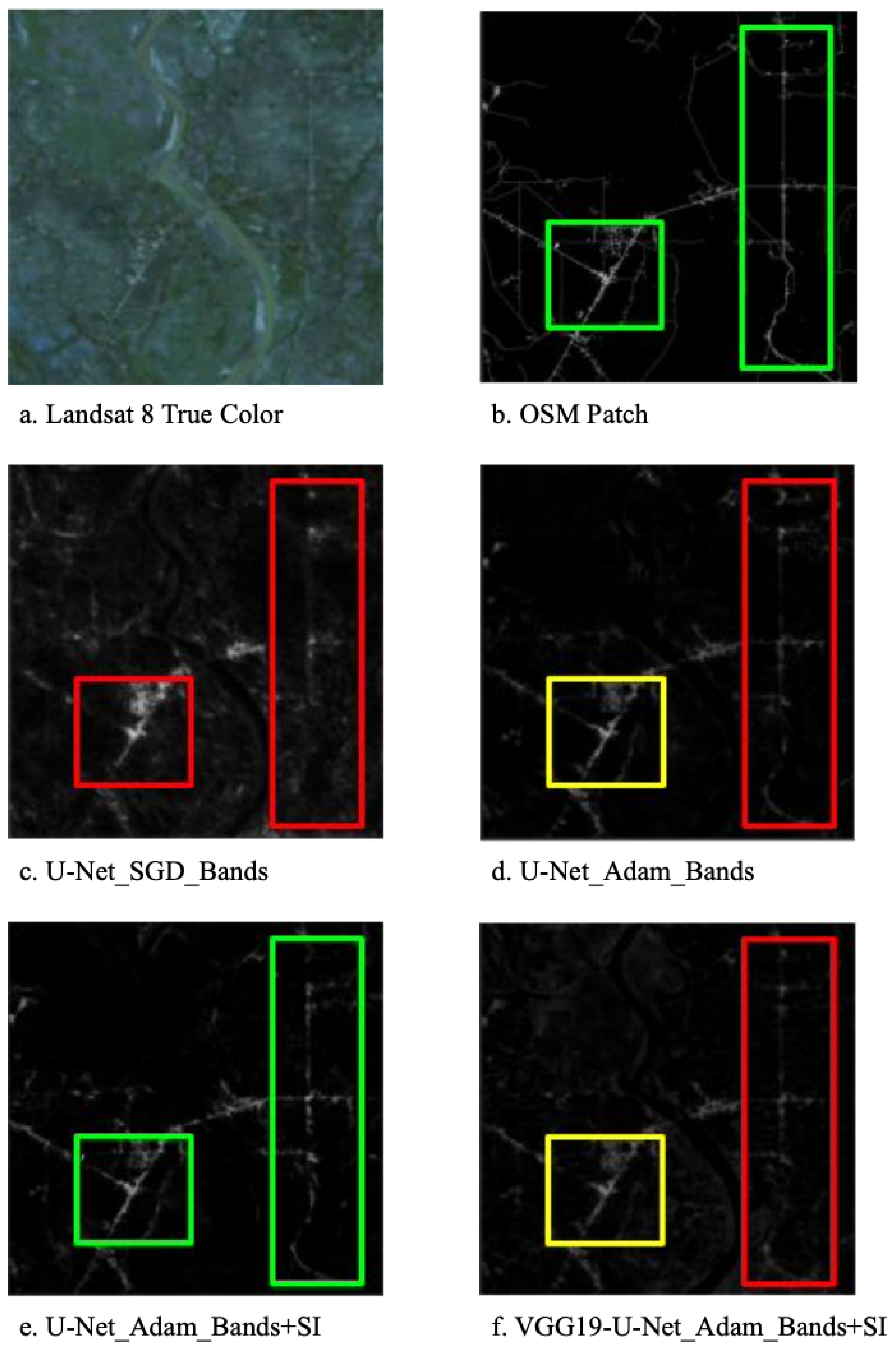
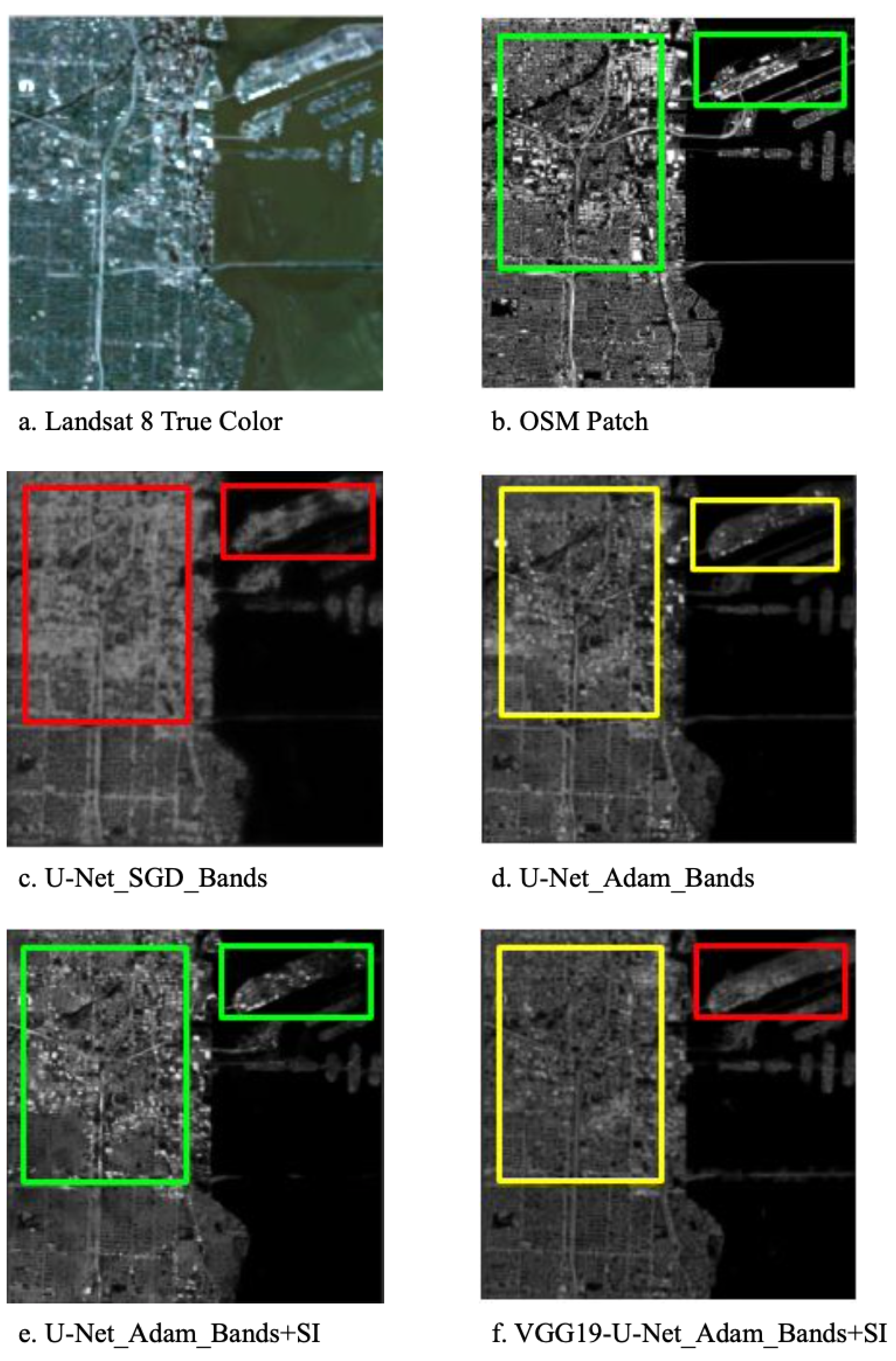
- U-Net_SGD_Bands: U-Net trained with Landsat 8 bands as features using the stochastic gradient descent (SGD) optimizer.
- U-Net_Adam_Bands: U-Net trained with Landsat 8 bands as features using the Adam optimizer.
- U-Net_Adam_Bands+SI: U-Net trained with Landsat 8 bands and four computed statistical indices as features using the Adam optimizer.
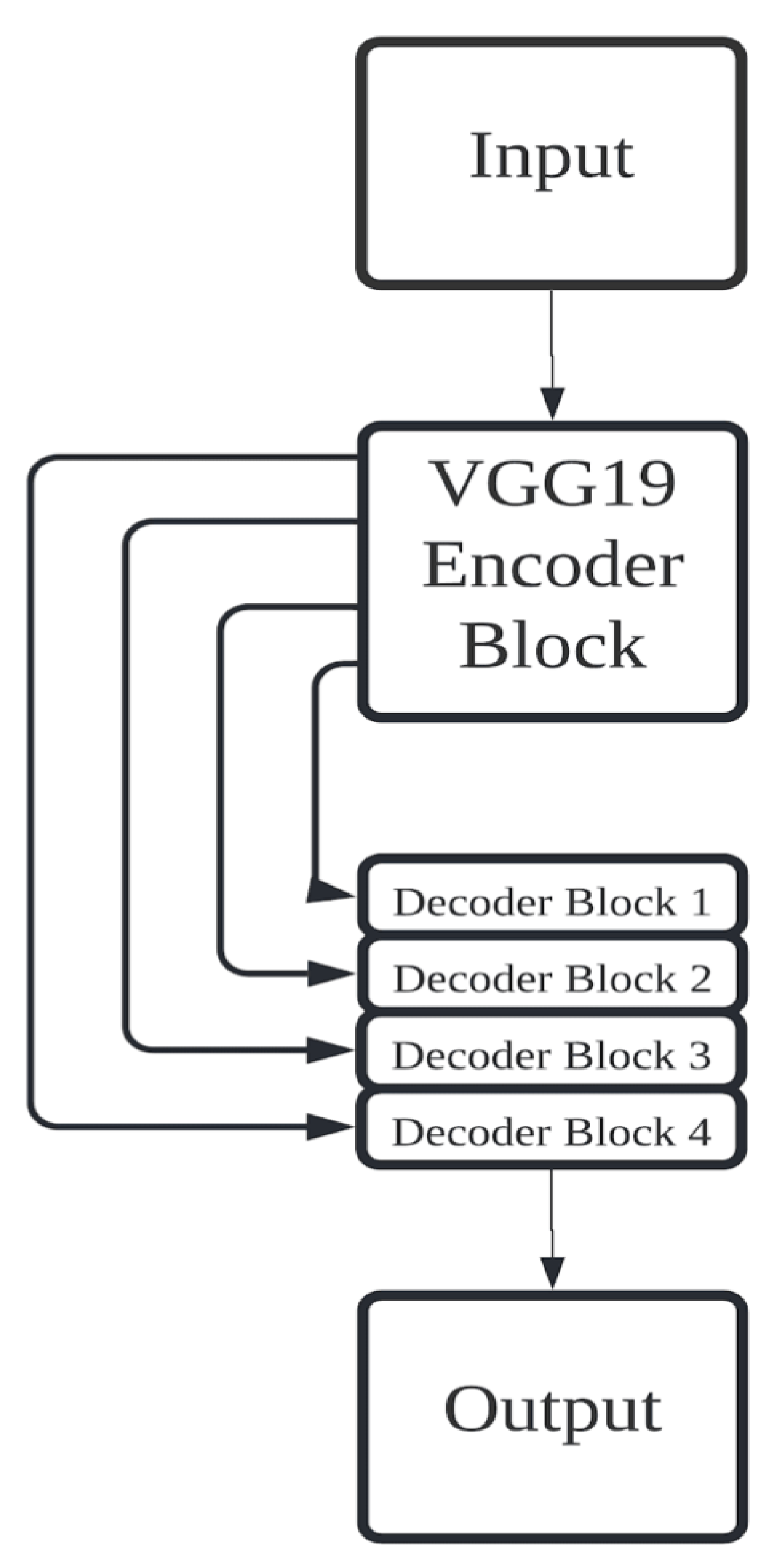
- VGG-19_Adam_Bands+SI: VGG-19-based encoder-decoder trained with Landsat 8 bands and computed statistical indices as features using the Adam optimizer.
3.5. Metrics
4. Results
4.1. Test Set Metrics
4.2. Test Set Image Observations
5. Discussion
6. Conclusions and Future Work
Author Contributions
Funding
Acknowledgments
Conflicts of Interest
References
- United Nations Department of Economic and Social Affairs (UN DESA). World’s Population Increasingly Urban with more than Half Living in Urban Areas. Available online: https://www.un.org/en/development/desa/news/population/world-urbanization-prospects-2014.html (accessed on 1 May 2021).
- Brabec, E.; Schulte, S.; Richards, P.L. Impervious surfaces and water quality: A review of current literature and its implications for watershed planning. J. Plan. Lit. 2002, 16, 499–514. [Google Scholar] [CrossRef]
- Radeloff, V.C.; Stewart, S.I.; Hawbaker, T.J.; Gimmi, U.; Pidgeon, A.M.; Flather, C.H.; Hammer, R.B.; Helmers, D.P. Housing growth in and near United States protected areas limits their conservation value. Proc. Natl. Acad. Sci. USA 2010, 107, 940–945. [Google Scholar] [CrossRef] [PubMed] [Green Version]
- Opoku, A. Biodiversity and the built environment: Implications for the Sustainable Development Goals (SDGs). Resour. Conserv. Recycl. 2019, 141, 1–7. [Google Scholar] [CrossRef]
- Arnfield, A.J. Two decades of urban climate research: A review of turbulence, exchanges of energy and water, and the urban heat island. Int. J. Climatol. A J. R. Meteorol. Soc. 2003, 23, 1–26. [Google Scholar] [CrossRef]
- Carlson, T.N.; Arthur, S.T. The impact of land use—land cover changes due to urbanization on surface microclimate and hydrology: A satellite perspective. Glob. Planet. Chang. 2000, 25, 49–65. [Google Scholar] [CrossRef]
- Seto, K.C.; Fragkias, M.; Güneralp, B.; Reilly, M.K. A meta-analysis of global urban land expansion. PLoS ONE 2011, 6, e23777. [Google Scholar] [CrossRef]
- Seto, K.C.; Parnell, S.; Elmqvist, T. A global outlook on urbanization. In Urbanization, Biodiversity and Ecosystem Services: Challenges and Opportunities; Springer: Dordrecht, The Netherlands, 2013; pp. 1–12. [Google Scholar]
- World Health Organization. The World Health Report, Life in the 21st Century, A Vision for All, Report of the Director-General. 1998. Available online: https://apps.who.int/iris/handle/10665/42065 (accessed on 1 May 2021).
- Moore, M.; Gould, P.; Keary, B.S. Global urbanization and impact on health. Int. J. Hyg. Environ. Health 2003, 206, 269–278. [Google Scholar] [CrossRef]
- Madhumathi, A.; Subhashini, S.; VishnuPriya, J. The Urban Heat Island Effect its Causes and Mitigation with Reference to the Thermal Properties of Roof Coverings. In Proceedings of the International Conference on Urban Sustainability: Emerging Trends Themes, Concepts & Practices (ICUS), Jaipur, India, 16–18 March 2018; Malaviya National Institute of Techonology: Jaipur, India, 2018. [Google Scholar]
- Polycarpou, L. No More Pavement! The Problem of Impervious Surfaces; State of the Planet, Columbia University Earth Institute: New York, NY, USA, 2010. [Google Scholar]
- Frazer, L. Paving Paradise: The Peril of Impervious Surfaces; National Institute of Environmental Health Sciences: Research Triangle Park, NC, USA, 2005; pp. A456–A462. [Google Scholar]
- Melesse, A.M.; Weng, Q.; Thenkabail, P.S.; Senay, G.B. Remote sensing sensors and applications in environmental resources mapping and modelling. Sensors 2007, 7, 3209–3241. [Google Scholar] [CrossRef] [Green Version]
- Liu, Z.; Wang, Y.; Li, Z.; Peng, J. Impervious surface impact on water quality in the process of rapid urbanization in Shenzhen, China. Environ. Earth Sci. 2013, 68, 2365–2373. [Google Scholar] [CrossRef]
- Kim, H.; Jeong, H.; Jeon, J.; Bae, S. The impact of impervious surface on water quality and its threshold in Korea. Water 2016, 8, 111. [Google Scholar] [CrossRef] [Green Version]
- Arnold, C.L., Jr.; Gibbons, C.J. Impervious surface coverage: The emergence of a key environmental indicator. J. Am. Plan. Assoc. 1996, 62, 243–258. [Google Scholar] [CrossRef]
- Roy, D.P.; Wulder, M.A.; Loveland, T.R.; Woodcock, C.E.; Allen, R.G.; Anderson, M.C.; Helder, D.; Irons, J.R.; Johnson, D.M.; Kennedy, R.; et al. Landsat-8: Science and product vision for terrestrial global change research. Remote Sens. Environ. 2014, 145, 154–172. [Google Scholar] [CrossRef] [Green Version]
- Saah, D.; Tenneson, K.; Poortinga, A.; Nguyen, Q.; Chishtie, F.; San Aung, K.; Markert, K.N.; Clinton, N.; Anderson, E.R.; Cutter, P.; et al. Primitives as building blocks for constructing land cover maps. Int. J. Appl. Earth Obs. Geoinf. 2020, 85, 101979. [Google Scholar] [CrossRef]
- Potapov, P.; Tyukavina, A.; Turubanova, S.; Talero, Y.; Hernandez-Serna, A.; Hansen, M.; Saah, D.; Tenneson, K.; Poortinga, A.; Aekakkararungroj, A.; et al. Annual continuous fields of woody vegetation structure in the Lower Mekong region from 2000–2017 Landsat time-series. Remote Sens. Environ. 2019, 232, 111278. [Google Scholar] [CrossRef]
- Poortinga, A.; Tenneson, K.; Shapiro, A.; Nquyen, Q.; San Aung, K.; Chishtie, F.; Saah, D. Mapping plantations in Myanmar by fusing Landsat-8, Sentinel-2 and Sentinel-1 data along with systematic error quantification. Remote Sens. 2019, 11, 831. [Google Scholar] [CrossRef] [Green Version]
- Schneider, A.; Friedl, M.A.; Potere, D. A new map of global urban extent from MODIS satellite data. Environ. Res. Lett. 2009, 4, 044003. [Google Scholar] [CrossRef] [Green Version]
- Saah, D.; Tenneson, K.; Matin, M.; Uddin, K.; Cutter, P.; Poortinga, A.; Nguyen, Q.H.; Patterson, M.; Johnson, G.; Markert, K.; et al. Land cover mapping in data scarce environments: Challenges and opportunities. Front. Environ. Sci. 2019, 7, 150. [Google Scholar] [CrossRef] [Green Version]
- Markert, K.N.; Markert, A.M.; Mayer, T.; Nauman, C.; Haag, A.; Poortinga, A.; Bhandari, B.; Thwal, N.S.; Kunlamai, T.; Chishtie, F.; et al. Comparing sentinel-1 surface water mapping algorithms and radiometric terrain correction processing in southeast asia utilizing google earth engine. Remote Sens. 2020, 12, 2469. [Google Scholar] [CrossRef]
- Poortinga, A.; Aekakkararungroj, A.; Kityuttachai, K.; Nguyen, Q.; Bhandari, B.; Soe Thwal, N.; Priestley, H.; Kim, J.; Tenneson, K.; Chishtie, F.; et al. Predictive Analytics for Identifying Land Cover Change Hotspots in the Mekong Region. Remote Sens. 2020, 12, 1472. [Google Scholar] [CrossRef]
- Phongsapan, K.; Chishtie, F.; Poortinga, A.; Bhandari, B.; Meechaiya, C.; Kunlamai, T.; Aung, K.S.; Saah, D.; Anderson, E.; Markert, K.; et al. Operational flood risk index mapping for disaster risk reduction using Earth Observations and cloud computing technologies: A case study on Myanmar. Front. Environ. Sci. 2019, 7, 191. [Google Scholar] [CrossRef] [Green Version]
- Poortinga, A.; Clinton, N.; Saah, D.; Cutter, P.; Chishtie, F.; Markert, K.N.; Anderson, E.R.; Troy, A.; Fenn, M.; Tran, L.H.; et al. An operational before-after-control-impact (BACI) designed platform for vegetation monitoring at planetary scale. Remote Sens. 2018, 10, 760. [Google Scholar] [CrossRef] [Green Version]
- Slonecker, E.T.; Jennings, D.B.; Garofalo, D. Remote sensing of impervious surfaces: A review. Remote Sens. Rev. 2001, 20, 227–255. [Google Scholar] [CrossRef]
- Bauer, M.E.; Heinert, N.J.; Doyle, J.K.; Yuan, F. Impervious surface mapping and change monitoring using Landsat remote sensing. In ASPRS Annual Conference Proceedings; American Society for Photogrammetry and Remote Sensing Bethesda: Rockville, MD, USA, 2004; Volume 10. [Google Scholar]
- Khanal, N.; Matin, M.A.; Uddin, K.; Poortinga, A.; Chishtie, F.; Tenneson, K.; Saah, D. A comparison of three temporal smoothing algorithms to improve land cover classification: A case study from NEPAL. Remote Sens. 2020, 12, 2888. [Google Scholar] [CrossRef]
- Weng, Q. (Ed.) Remote Sensing of Impervious Surfaces; CRC Press: Boca Raton, FL, USA, 2007. [Google Scholar]
- Liu, Z.; Wang, Y.; Peng, J. Remote sensing of impervious surface and its applications: A review. Prog. Geogr. 2010, 29, 1143–1152. [Google Scholar]
- Wang, Y.; Li, M. Urban impervious surface detection from remote sensing images: A review of the methods and challenges. IEEE Geosci. Remote Sens. Mag. 2019, 7, 64–93. [Google Scholar] [CrossRef]
- Pettorelli, N. The Normalized Difference Vegetation Index; Oxford University Press: Oxford, UK, 2013. [Google Scholar]
- Zha, Y.; Gao, J.; Ni, S. Use of normalized difference built-up index in automatically mapping urban areas from TM imagery. Int. J. Remote Sens. 2003, 24, 583–594. [Google Scholar] [CrossRef]
- Xu, H. Analysis of impervious surface and its impact on urban heat environment using the Normalized Difference Impervious Surface Index (NDISI). Photogramm. Eng. Remote Sens. 2010, 76, 557–565. [Google Scholar] [CrossRef]
- Liu, C.; Shao, Z.; Chen, M.; Luo, H. MNDISI: A multi-source composition index for impervious surface area estimation at the individual city scale. Remote Sens. Lett. 2013, 4, 803–812. [Google Scholar] [CrossRef]
- Deng, C.; Wu, C. BCI: A biophysical composition index for remote sensing of urban environments. Remote Sens. Environ. 2012, 127, 247–259. [Google Scholar] [CrossRef]
- Tian, Y.; Chen, H.; Song, Q.; Zheng, K. A novel index for impervious surface area mapping: Development and validation. Remote Sens. 2018, 10, 1521. [Google Scholar] [CrossRef] [Green Version]
- Masek, J.; Lindsay, F.; Goward, S. Dynamics of urban growth in the Washington DC metropolitan area, 1973–1996, from Landsat observations. Int. J. Remote Sens. 2000, 21, 3473–3486. [Google Scholar] [CrossRef]
- Shi, L.; Ling, F.; Ge, Y.; Foody, G.M.; Li, X.; Wang, L.; Zhang, Y.; Du, Y. Impervious surface change mapping with an uncertainty-based spatial-temporal consistency model: A case study in Wuhan City using Landsat time-series datasets from 1987 to 2016. Remote Sens. 2017, 9, 1148. [Google Scholar] [CrossRef] [Green Version]
- Hu, X.; Weng, Q. Estimating impervious surfaces from medium spatial resolution imagery using the self-organizing map and multi-layer perceptron neural networks. Remote Sens. Environ. 2009, 113, 2089–2102. [Google Scholar] [CrossRef]
- Zhang, Y.; Zhang, H.; Lin, H. Improving the impervious surface estimation with combined use of optical and SAR remote sensing images. Remote Sens. Environ. 2014, 141, 155–167. [Google Scholar] [CrossRef]
- Bauer, M.E.; Loffelholz, B.C.; Wilson, B. Estimating and mapping impervious surface area by regression analysis of Landsat imagery. In Remote Sensing of Impervious Surfaces; CRC Press: Boca Raton, FL, USA, 2008; pp. 3–19. [Google Scholar]
- Map, O.S. Open street map. Retr. March 2014, 18, 2014. [Google Scholar]
- Wang, J.; Wu, Z.; Wu, C.; Cao, Z.; Fan, W.; Tarolli, P. Improving impervious surface estimation: An integrated method of classification and regression trees (CART) and linear spectral mixture analysis (LSMA) based on error analysis. GIScience Remote Sens. 2018, 55, 583–603. [Google Scholar] [CrossRef]
- Curlander, J.C.; McDonough, R.N. Synthetic Aperture Radar; Wiley: New York, NY, USA, 1991. [Google Scholar]
- Zhang, X.; Du, S. A Linear Dirichlet Mixture Model for decomposing scenes: Application to analyzing urban functional zonings. Remote Sens. Environ. 2015, 169, 37–49. [Google Scholar] [CrossRef]
- LeCun, Y.; Bengio, Y.; Hinton, G. Deep learning. Nature 2015, 521, 436–444. [Google Scholar] [CrossRef]
- LeCun, Y.; Bottou, L.; Bengio, Y.; Haffner, P. Gradient-based learning applied to document recognition. Proc. IEEE 1998, 86, 2278–2324. [Google Scholar] [CrossRef] [Green Version]
- Dargan, S.; Kumar, M.; Ayyagari, M.R.; Kumar, G. A survey of deep learning and its applications: A new paradigm to machine learning. Arch. Comput. Methods Eng. 2019, 27, 1071–1092. [Google Scholar] [CrossRef]
- Noh, H.; Hong, S.; Han, B. Learning deconvolution network for semantic segmentation. In Proceedings of the IEEE International Conference on Computer Vision, Santiago, Chile, 7–13 December 2015; pp. 1520–1528. [Google Scholar]
- Szeliski, R. Computer Vision: Algorithms and Applications; Springer Science & Business Media: Berlin/Heidelberg, Germany, 2010. [Google Scholar]
- Minaee, S.; Boykov, Y.; Porikli, F.; Plaza, A.; Kehtarnavaz, N.; Terzopoulos, D. Image segmentation using deep learning: A survey. arXiv 2020, arXiv:2001.05566. [Google Scholar]
- Badrinarayanan, V.; Kendall, A.; Cipolla, R. Segnet: A deep convolutional encoder-decoder architecture for image segmentation. IEEE Trans. Pattern Anal. Mach. Intell. 2017, 39, 2481–2495. [Google Scholar] [CrossRef]
- Ronneberger, O.; Fischer, P.; Brox, T. U-net: Convolutional networks for biomedical image segmentation. In Proceedings of the International Conference on Medical Image Computing and Computer-Assisted Intervention, Munich, Germany, 5–9 October 2015; Springer: Munich, Germany, 2015; pp. 234–241. [Google Scholar]
- Russakovsky, O.; Deng, J.; Su, H.; Krause, J.; Satheesh, S.; Ma, S.; Huang, Z.; Karpathy, A.; Khosla, A.; Bernstein, M.; et al. Imagenet large scale visual recognition challenge. Int. J. Comput. Vis. 2015, 115, 211–252. [Google Scholar] [CrossRef] [Green Version]
- Simonyan, K.; Zisserman, A. Very deep convolutional networks for large-scale image recognition. arXiv 2014, arXiv:1409.1556. [Google Scholar]
- Szegedy, C.; Liu, W.; Jia, Y.; Sermanet, P.; Reed, S.; Anguelov, D.; Erhan, D.; Vanhoucke, V.; Rabinovich, A. Going deeper with convolutions. In Proceedings of the IEEE Conference on Computer Vision and Pattern Recognition, Boston, MA, USA, 8–10 June 2015; pp. 1–9. [Google Scholar]
- He, K.; Zhang, X.; Ren, S.; Sun, J. Deep residual learning for image recognition. In Proceedings of the IEEE Conference on Computer Vision and Pattern Recognition, Las Vegas, NV, USA, 27–30 June 2016; pp. 770–778. [Google Scholar]
- He, K.; Zhang, X.; Ren, S.; Sun, J. Delving deep into rectifiers: Surpassing human-level performance on imagenet classification. In Proceedings of the IEEE International Conference on Computer Vision, Santiago, Chile, 7–13 December 2015; pp. 1026–1034. [Google Scholar]
- Ioffe, S.; Szegedy, C. Batch normalization: Accelerating deep network training by reducing internal covariate shift. In Proceedings of the International Conference on Machine Learning, PMLR, Lille, France, 7–9 July 2015; pp. 448–456. [Google Scholar]
- Nair, V.; Hinton, G.E. Rectified Linear Units Improve Restricted Boltzmann Machines. In Proceedings of the 27th International Conference on Machine Learning (ICML-10), Haifa, Israel, 21–24 June 2010. [Google Scholar]
- Tompson, J.; Goroshin, R.; Jain, A.; LeCun, Y.; Bregler, C. Efficient object localization using convolutional networks. In Proceedings of the IEEE Conference on Computer Vision and Pattern Recognition, Boston, MA, USA, 7–12 June 2015; pp. 648–656. [Google Scholar]
- An, G. The effects of adding noise during backpropagation training on a generalization performance. Neural Comput. 1996, 8, 643–674. [Google Scholar] [CrossRef]
- Srivastava, N.; Hinton, G.; Krizhevsky, A.; Sutskever, I.; Salakhutdinov, R. Dropout: A simple way to prevent neural networks from overfitting. J. Mach. Learn. Res. 2014, 15, 1929–1958. [Google Scholar]
- Wang, Q.; Ma, Y.; Zhao, K.; Tian, Y. A comprehensive survey of loss functions in machine learning. Ann. Data Sci. 2020, 1–26. [Google Scholar] [CrossRef]
- Bottou, L.; Curtis, F.E.; Nocedal, J. Optimization methods for large-scale machine learning. Siam Rev. 2018, 60, 223–311. [Google Scholar] [CrossRef]
- Kingma, D.P.; Ba, J. Adam: A method for stochastic optimization. arXiv 2014, arXiv:1412.6980. [Google Scholar]
- Ruder, S. An overview of gradient descent optimization algorithms. arXiv 2016, arXiv:1609.04747. [Google Scholar]
- Gorelick, N.; Hancher, M.; Dixon, M.; Ilyushchenko, S.; Thau, D.; Moore, R. Google Earth Engine: Planetary-scale geospatial analysis for everyone. Remote Sens. Environ. 2017, 202, 18–27. [Google Scholar] [CrossRef]
- Abadi, M.; Barham, P.; Chen, J.; Chen, Z.; Davis, A.; Dean, J.; Devin, M.; Ghemawat, S.; Irving, G.; Isard, M.; et al. Tensorflow: A system for large-scale machine learning. In Proceedings of the 12th USENIX Symposium on Operating Systems Design and Implementation (OSDI’16), Savannah, GA, USA, 2–4 November 2016; pp. 265–283. [Google Scholar]
- Carneiro, T.; Da Nóbrega, R.V.M.; Nepomuceno, T.; Bian, G.B.; De Albuquerque, V.H.C.; Reboucas Filho, P.P. Performance analysis of google colaboratory as a tool for accelerating deep learning applications. IEEE Access 2018, 6, 61677–61685. [Google Scholar] [CrossRef]


| Model Names | Evaluation RMSE | Test RMSE | Test Accuracy |
|---|---|---|---|
| U-Net_SGD_Bands | 0.1587 | 0.1582 | 90.87% |
| U-Net_Adam_Bands | 0.1356 | 0.1358 | 92.28% |
| U-Net_Adam_Bands+SI | 0.1360 | 0.1375 | 92.46% |
| VGG19_Adam_Bands+SI | 0.1525 | 0.1582 | 90.11% |
Publisher’s Note: MDPI stays neutral with regard to jurisdictional claims in published maps and institutional affiliations. |
© 2021 by the authors. Licensee MDPI, Basel, Switzerland. This article is an open access article distributed under the terms and conditions of the Creative Commons Attribution (CC BY) license (https://creativecommons.org/licenses/by/4.0/).
Share and Cite
Parekh, J.R.; Poortinga, A.; Bhandari, B.; Mayer, T.; Saah, D.; Chishtie, F. Automatic Detection of Impervious Surfaces from Remotely Sensed Data Using Deep Learning. Remote Sens. 2021, 13, 3166. https://doi.org/10.3390/rs13163166
Parekh JR, Poortinga A, Bhandari B, Mayer T, Saah D, Chishtie F. Automatic Detection of Impervious Surfaces from Remotely Sensed Data Using Deep Learning. Remote Sensing. 2021; 13(16):3166. https://doi.org/10.3390/rs13163166
Chicago/Turabian StyleParekh, Jash R., Ate Poortinga, Biplov Bhandari, Timothy Mayer, David Saah, and Farrukh Chishtie. 2021. "Automatic Detection of Impervious Surfaces from Remotely Sensed Data Using Deep Learning" Remote Sensing 13, no. 16: 3166. https://doi.org/10.3390/rs13163166
APA StyleParekh, J. R., Poortinga, A., Bhandari, B., Mayer, T., Saah, D., & Chishtie, F. (2021). Automatic Detection of Impervious Surfaces from Remotely Sensed Data Using Deep Learning. Remote Sensing, 13(16), 3166. https://doi.org/10.3390/rs13163166