Article

Analysis of Wetland Landcover Change in Great Lakes Urban Areas Using Self-Organizing Maps

1
Yeates School of Graduate Studies, Ryerson University, Toronto, ON M5B 2K3, Canada
2
Department of Geography and Environmental Studies, Ryerson University, Toronto, ON M5B 2K3, Canada
*
Author to whom correspondence should be addressed.
Remote Sens. 2021, 13(24), 4960; https://doi.org/10.3390/rs13244960
Submission received: 16 November 2021 / Revised: 30 November 2021 / Accepted: 3 December 2021 / Published: 7 December 2021
(This article belongs to the Special Issue Machine Learning Techniques Applied to Geosciences and Remote Sensing)

Abstract

:
Wetland loss and subsequent reduction of wetland ecosystem services in the Great Lakes region has been driven, in part, by changing landcover and increasing urbanization. With landcover change data, digital elevation models (DEM), and self-organizing maps (SOM), this study explores changing landcover and the flood mitigation attributes of wetland areas over a 15-year period in Toronto and Chicago. The results of this analysis show that (1) in the city of Toronto SOM clusters, the landcover change correlations with wetland volume and wetland area range between −0.1 to −0.5, indicating that a more intense landcover change tends to be correlated with small shallow wetlands, (2) in the city of Chicago SOM clusters, the landcover change correlations with wetland area range between −0.1 to −0.7, the landcover change correlations with wetland volume per area range between −0.1 to 0.8, and the landcover change correlations with elevation range between −0.2 to −0.6, indicating that more intense landcover change tends to be correlated with spatially small wetlands that have a relatively high water-storage capacity per area and are located at lower elevations. In both cities, the smallest SOM clusters represent wetland areas where increased landcover change is correlated with wetland areas that have high flood mitigation potential. This study aims to offer a new perspective on changing urban landscapes and urban wetland ecosystem services in Toronto and Chicago.

1. Introduction

Laurentian Great Lake wetlands provide several vital ecosystem services, including wildlife habitat, water filtration, sediment retention, carbon sequestration, erosion prevention, and flood mitigation [1,2]. Both riparian and inland wetlands are able to mitigate the impacts of flooding events through water storage (riparian wetlands) and peak flow attenuation (inland wetlands) [3,4]. Wetland loss, degradation, and fragmentation is widespread throughout North America and is, in part, cause by land conversion, urban development, and transportation [5]. As wetland areas are lost or converted via urban development, and population density increases, the per capita value of wetland ecosystem services will often rise, and the ecosystem services that wetlands offer are challenging and sometimes impossible to fully replace or replicate once wetlands have been lost [6].
This study uses self-organizing maps (SOM) to explore changing landcover and the flood mitigation attributes of wetland areas over a 15-year period in two Great Lakes urban areas, Toronto and Chicago. Landcover datasets and high-resolution digital elevation models have been used to measure several different attributes of the wetlands in these urban areas, including wetland volume, wetland area, wetland volume per area, drainage area, and average elevation. The wetland attributes and ranked intensity of landcover change were included in the SOM analysis, and subsequent correlation matrices were produced for each SOM cluster. The results of this study (1) provide insights into how the changing landcover of wetlands areas may alter wetland flood mitigation potential, and (2) identify wetland areas where protection and restoration efforts would likely improve flood mitigation potential. This study aims to contribute a novel and innovative methodological approach, which uses GIS and machine learning to provide new perspectives on how landcover change can influence wetlands as flood mitigation tools in the Great Lakes urban areas.
Research on the link between landcover change and wetland water quality in the Great Lakes region has shown that as urbanization increases in and around wetland areas, there is a decrease in the water quality of the wetlands. Additionally, increasing natural landcover around wetland areas is shown to have positive impacts on water quality throughout the watershed, and increasing natural landcover around up-river wetlands positively impacts the water quality of the coastal and riparian wetlands down-river [7]. Increasing development in the Great Lakes watersheds has also been shown to impact ecological communities of coastal wetlands by increasing sediment discharge, pollutants, impervious surface areas, and habitat destruction [8].
In both Toronto and Chicago, landcover change and urbanization has impacted wetlands and facilitated wetland loss. Over the past ~200 years, southern Ontario wetlands have experienced an estimated loss of more than 68%, and since the early 1980s wetland loss in Toronto and the greater Toronto area has primarily been driven by urbanization [9,10]. Additionally, over the past 150 years, wetland loss has been a major feature of landcover change in the state of Illinois, with 85% of wetlands lost in the state during this time period. In the Chicago region, urbanization has facilitated wetland loss, reducing both the quality and area of wetlands in the region [11].
Wetlands provide several critical ecosystem services, including flood mitigation and reduction services through water detention and retention. The impacts of flooding can be reduced in neighbouring areas because wetlands are able to hold water and retain comparatively high water tables [12]. Depressional wetlands can reduce peak flows during snow melt and precipitation events, and prioritising the protection of larger depressional wetlands, while allowing the loss of smaller wetlands may impact the functions, integrity, and resilience of the watershed [13]. The spatial scale of the wetland benefits is also important to acknowledge, as wetlands that are spatially situated away from areas that experience flooding may still be providing benefits and reducing the impacts of the flood [14]. Generally, the benefits of wetlands that act as a flood reduction service are defined by upstream and downstream landscape characteristics [15]. As the impacts associated with climate change become more prominent, utilizing wetlands as a component of flood control in the Great Lakes region will be particularly important [16].
There have been four major flooding events in the city of Toronto in the past 100 years, (occurring in 1954, 1976, 2005, and 2013), and climate change is projected to impact the likelihood of more frequent flooding [17]. A 2016 study showed that non-stationary conditions resulting from climate change impact the intensity-duration-frequency (IDF) curves of historical precipitation data in the Province of Ontario. This study shows that, due to climate change, the intensity, duration, and frequency of precipitation events are already changing in Ontario and will continue to change if environmental changes associated with climate change continue [18]. In the city of Chicago, there have been 13 significant flooding events since 1848 (occurring in 1848, 1855, 1885, 1938, 1952, 1954, 1957, 1961, 1973, 1979, 1986, 1987, and 1996) and evidence suggests that as metropolitan Chicago has continued to expand and develop, the magnitude of the floods has increased [19].
Self-organizing maps have a broad number of applications and SOM have been widely used in ecological and environmental research to better understand complex systems at both small and large scales [20]. SOM’s have been used in wetland research and landcover change research to predict performance of constructed wetland agro-ecosystems, predict concentrations of heavy metals in constructed wetlands, pattern vegetation community types in coastal wetlands, and investigate changes in spatiotemporal landcover patterns [21,22,23,24].

2. Materials and Methods

SOM algorithms map high-dimensional data patterns to an output space or n-dimensional grid where this output space is usually two-dimensional, and the grid of units may be rectangular or hexagonal [25]. This process is an unsupervised machine learning technique, which preserves the topological relationships within the dataset, and broadly, requires two steps, training and mapping. The training process of a SOM creates a two-dimensional input space comprised of neurons (or nodes), and the distance between the dataset neurons and the input space pattern is determined. The neurons that are closest to the input space pattern are selected as winning neurons. The mapping process takes the input space pattern and maps it to the winning neurons, or to other close neurons in the output space. SOM is useful for examining and grouping high dimensional data into clusters, as well as visualizing the analysis through topological maps, and in this study, applying the SOM results to spatial maps [26,27]. For a more detailed description of the SOM algorithm the reader is referred to [28].
Measuring wetland landcover change between 2000 and 2015 in the city of Toronto required two datasets: the Southern Ontario Land Resource Information System (2000–2002) v1.1 GeoTiff and the Southern Ontario Land Resource Information System (SOLRIS) 3.0 GeoTiff. Measuring wetland landcover change between 2001 and 2016 in the city of Chicago also required two datasets: the NLCD 2001 Land Cover (CONUS) GeoTiff, and the NLCD 2016 Land Cover (CONUS) GeoTiff. The 2000 and 2015 SOLRIS (southern Ontario) GeoTiff images were added to QGIS and clipped to the city of Toronto boundary, and the 2001 and 2015 CONUS (Contiguous United States) were also added to QGIS and clipped to the city of Chicago boundary.
The semi-automatic classification plugin was used to determine the changes in pixel classification between 2000 and 2015 (Toronto) and 2001–2016 (Chicago). The GeoTiff landcover change image pixels were reclassified to show only the areas that were classified as wetlands in 2000 (Toronto) and 2001 (Chicago). This was done by reclassifying the pixel values where the reference value was classified as a wetland, and the new pixel value was classified based on the reclass value result from the landcover change analysis. The results of this analysis included GeoTiff images that showed the locations of wetlands as of 2000 (Toronto) and 2001 (Chicago), where the pixel classification was the landcover class as of 2015 and 2016.
The new wetland landcover change GeoTiff images were vectorized and saved as shapefiles. An additional field was added to the attribute table of the wetland landcover change shapefile. This field included a numerical ranking system (labelled as ‘LCC Code’ in the figures) for the landcover change based on the intensification of change that occurred for each feature in the wetland landcover change shapefile. This was done so that the landcover change values could be included in the SOM analysis. All the landcover change classifications were ranked between 1 and 5, where higher values (5) denoted more intense change and lower water retention capacity and lower values (1) denoted no change and higher water retention capacity. The landcover change ranking system is outlined in Table 1 (Toronto) and Table 2 (Chicago).
The 2000 (Toronto) and 2001 (Chicago) wetland area and volume were calculated with the vectorized wetland landcover change (wetland polygon) shapefiles. This analysis required two additional datasets, a 5 m resolution greater Toronto area (GTA) Digital Elevation Model 2002 and two 10 m resolution USGS Digital Elevation Models. The wetland polygon shapefiles and DEM images were overlaid in QGIs. The minimum and maximum values of the DEM, and the number of pixels (count) spatially associated with each wetland polygon, were calculated using the zonal statistics algorithm. This process added the minimum elevation, maximum elevation, and number of DEM pixels to the attribute table of the vectorized wetland landcover change polygon shapefile. The formula used to calculate the water storage capacity volume of the wetland depressional areas was pulled from a 2017 study that used LiDAR and aerial imagery to model the hydrologic connectivity of wetlands [29].
V = i = 1 n ( C Z i ) · R 2
where C is the maximum elevation (m) of the wetland depression, Zi is the elevation of pixel i (m), R is the spatial resolution of the DEM (m), and n is the number of pixels that fall within the wetland depression area. This formula was applied to all the wetland polygons using the field calculator, the volume in m3 was added as a new column to the attribute table and the values (m3) were converted to dam3. The area of the wetland polygons was also calculated in the field calculator as m2 and converted to dam2.
Drainage areas for the Toronto and Chicago wetland polygons were calculated to determine the area in dam2 where rainfall and water runoff will flow into each wetland polygon. Drainage areas were calculated using the GRASS r.watershed algorithm and the high-resolution DEM images, with the minimum size of the exterior watershed basin set to 40,000 pixels for Toronto and 20,000 for Chicago. This process produced a new raster image where pixel values denoted the number of pixels that drain through each pixel.
The drainage area for each wetland polygon was determined by (1) overlaying the wetland polygon shapefile and drainage area raster image, (2) calculating the sum of the drainage pixel values and the number of drainage pixels (count), spatially associated with each wetland polygon using the zonal statistics algorithm, and (3) applying the following formula in the wetland polygon attribute table field calculator.
D A = L 2 ( S C )
where DA is the drainage area (m2), L is the resolution of the drainage area raster image (m), S is the sum of the pixel values overlapping each wetland polygon, and C is the number of pixels overlapping each wetland polygon. The area in m2 was added as a new column to the attribute table and the values (m2) were converted to dam2.
The attribute tables of the 2000 (Toronto) and 2001 (Chicago) wetland polygon shapefiles included (1) the 2015 (Toronto) and 2016 (Chicago) landcover change (ranking) code (i.e., the 2015 (Toronto) and 2016 (Chicago) landcover change ranking, denoting the intensification of change that occurred for the areas that as of 2000 (Toronto) and 2001 (Chicago) were classified as wetlands), (2) the area of each wetland polygon (dam2), (3) the volume of each wetland polygon (dam3), (4) the drainage area (dam2) for each wetland polygon, and (5) the average elevation of each wetland polygon (calculated from the DEM zonal statistics, where the zones were each wetland polygon). The attribute tables were exported as spreadsheets and were used in the SOM analysis. To avoid a small number of spatially large wetland systems skewing the result of the SOM analysis, the wetland area (dam2) and wetland volume (dam
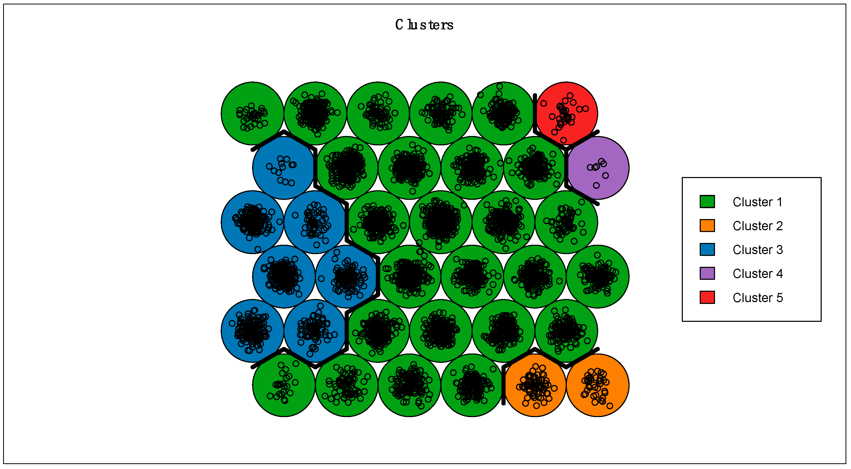
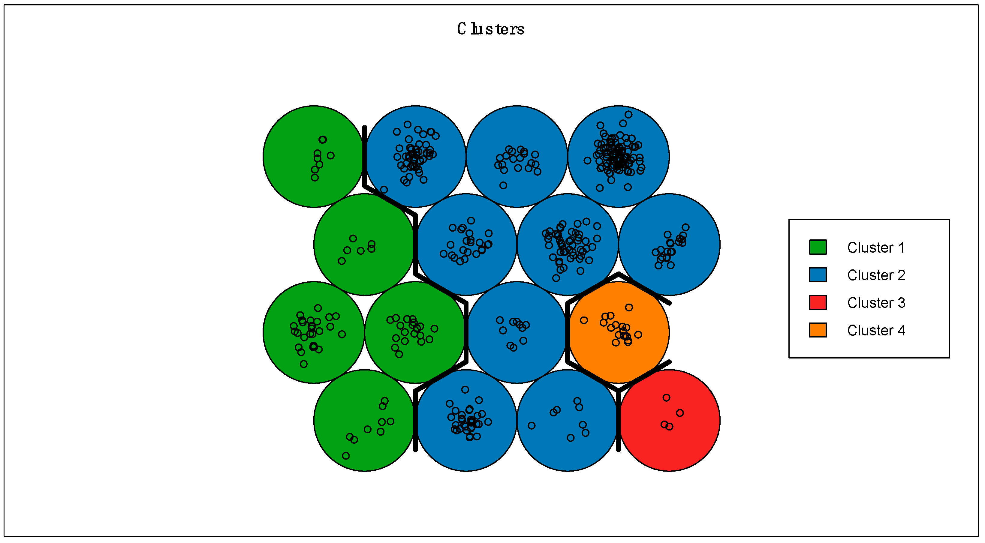
3) data were converted to wetland volume/area (dam). The SOM analysis was conducted in R, and the Toronto and Chicago data were mapped in two separate SOM analysis. The Toronto and Chicago data were normalized and due to differences in the size of the datasets, the Toronto data were mapped on a 6 × 6 hexagonal grid with 5 clusters and the Chicago data were mapped on a 4 × 4 hexagonal grid with 4 clusters. The R script used to conduct the SOM analysis is included in the Supplementary Materials (Toronto_Wetland_SOM.R and Chicago_Wetland_SOM.R).
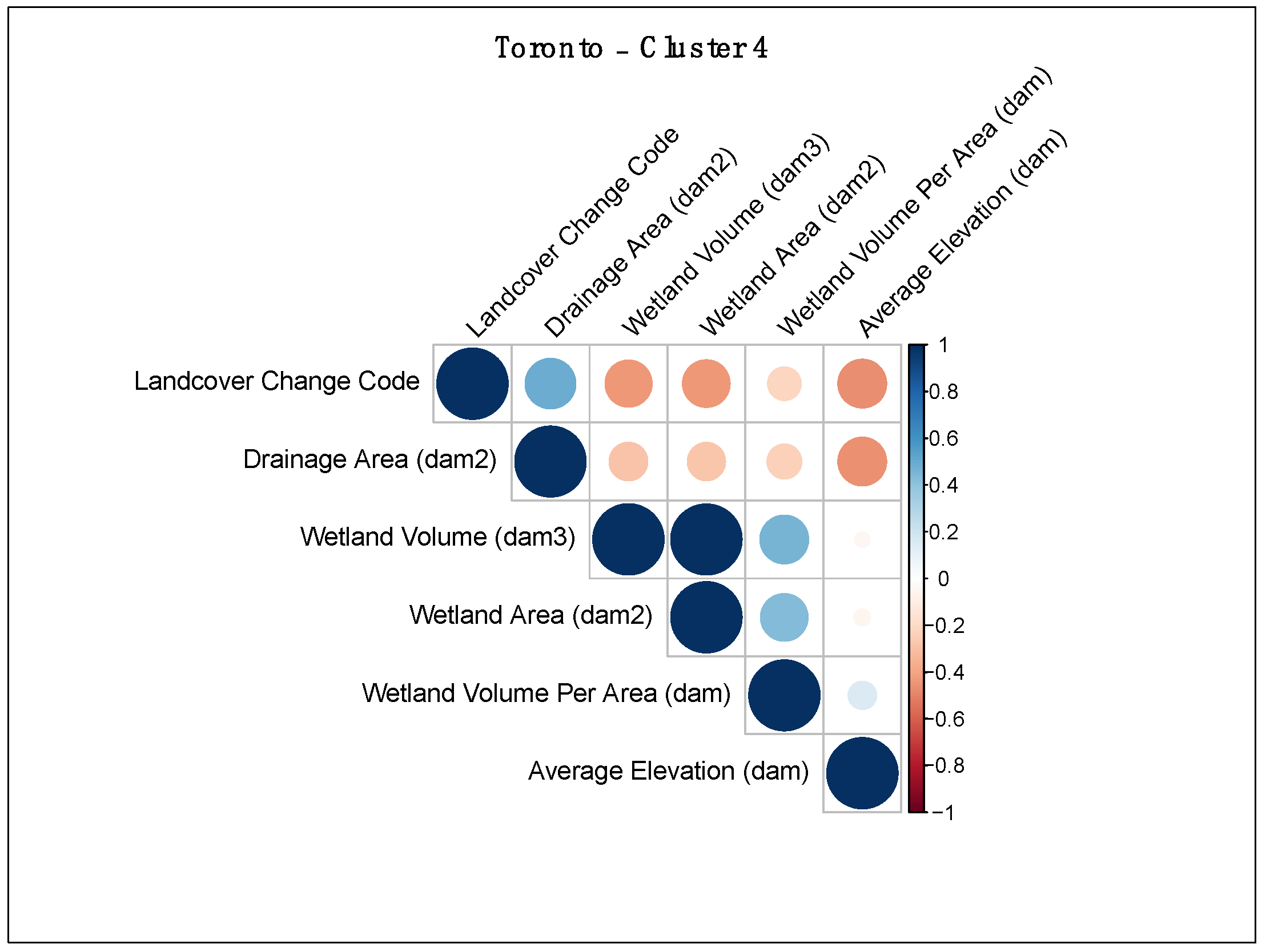
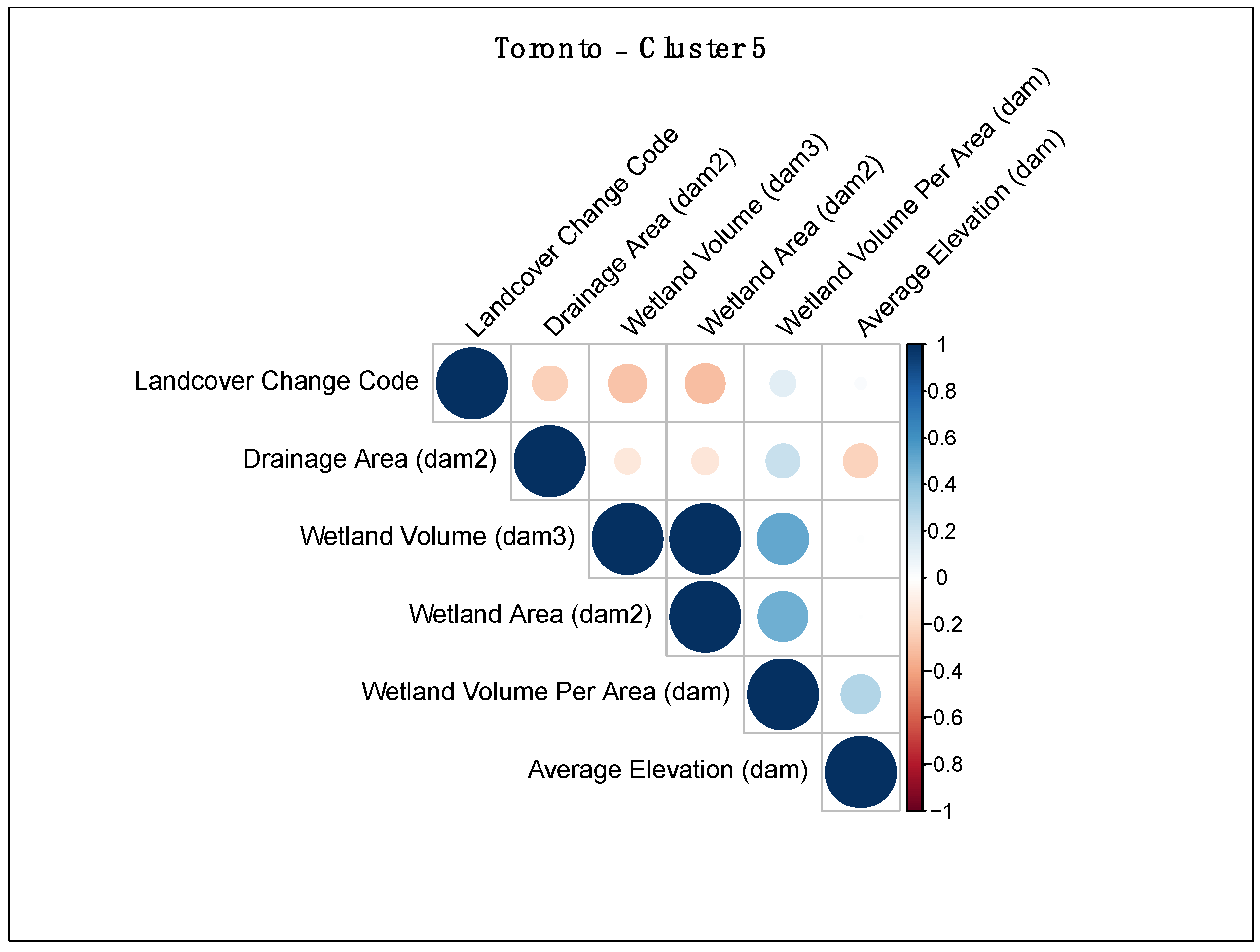
The correlation coefficients of the SOM analysis results were calculated for each cluster and were used to create correlation matrices. The wetland area (dam2) and wetland volume (dam3) data were included in the correlation matrices so that these wetland attributes could be compared to the attributes included in the SOM analysis and enhance the discussion of the study results. It is acknowledged that the large wetland outliers slightly skewed the correlation between the wetland area (dam2) and wetland volume (dam3), and other wetland attributes included in the correlation matrices. However, their inclusion in this analysis does not retract from the correlation comparison of the remaining wetland attributes and the wetland volume/area (dam) attribute was retained in this analysis. The R script used to calculate the correlation coefficients of the SOM analysis are included in the Supplementary Materials (Correlation_Matrix_Code.R).
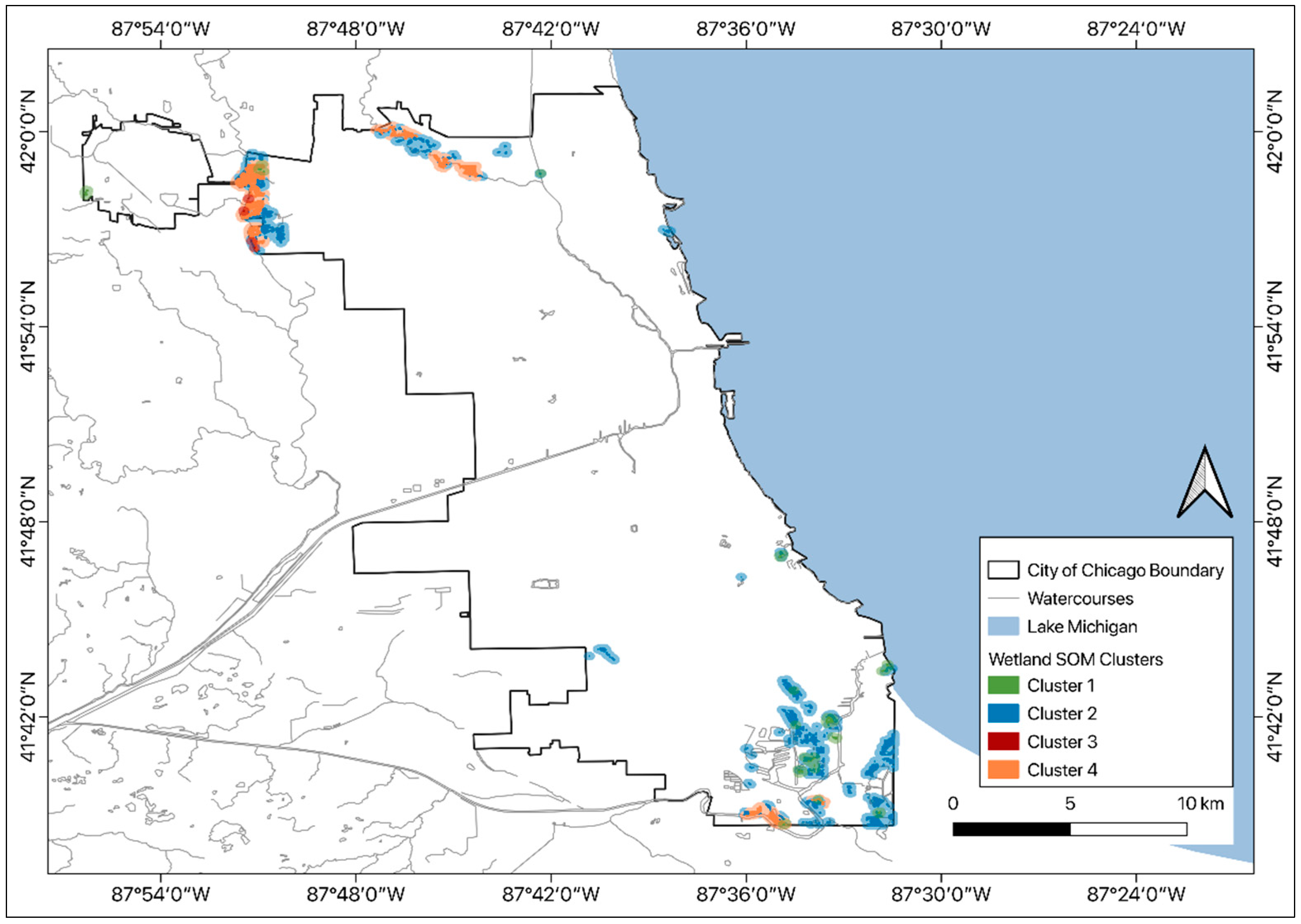
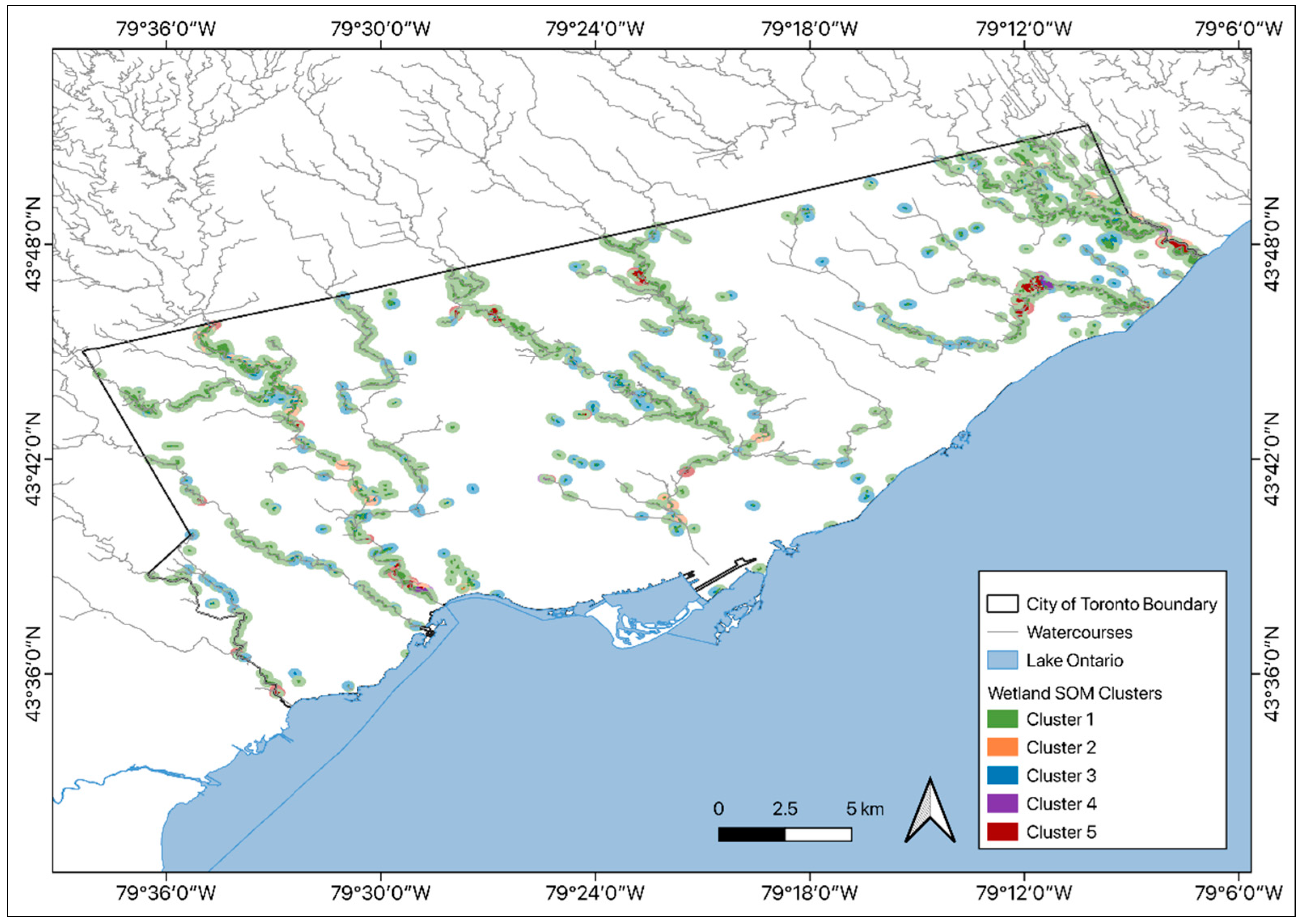
The SOM clusters were added to the wetland shapefiles attribute tables, which were used to produce maps for Toronto and Chicago displaying the wetland areas (as of 2000 and 2001). Colours of the wetland polygons were changed to reflect their SOM cluster classification. A 200-m buffer was added to each polygon and the opacity of the buffer was reduced to 50%. This was done to enhance the visualization of the maps and ensure that small wetland polygons were visible. All GIS analysis and map creation was completed in QGIS 3.14. The SOM analysis and correlation matrices were completed in R [30,31].

3. Results

3.1. City of Toronto

The results of the SOM analysis for the city of Toronto are included in Figure 1. Clusters 1 and 3 are the dominant clusters, with the highest number of wetland polygons included in cluster 1. Cluster 2 has a moderately high number of wetland polygons. Clusters 4 and 5 have the lowest number of wetland polygons, with very few wetland polygons included in cluster 4. In the following correlation matrices, the colour and size of the circles describe the level of correlation between the wetland attributes in each SOM cluster. Larger and darker circles illustrate stronger correlational relationships and smaller, lighter circles illustrate weaker correlational relationships. Blue circles illustrate a positive correlational relationship and red circles illustrate negative correlational relationships.
The correlation matrix for Cluster 1 (Figure 2) shows that (1) landcover change has a weak negative correlation with wetland volume, wetland area, and volume per area, indicating that wetland areas where more intense landcover change has occurred tend to be areas with smaller, shallow wetlands that have a lower water storage capacity per area. (2) Drainage area has a weak positive correlation with wetland volume per area, indicating that in this cluster, during rain events, more water tends to flow into wetlands with a higher water storage capacity per area. For the city of Toronto, this correlation matrix (Cluster 1), as well as in the correlation matrices for clusters 2–5, wetland volume, wetland area, and wetland volume per area are positively correlated.
The correlation matrix for Cluster 2 (Figure 3) shows that (1) landcover change has a weak negative correlation with wetland volume and wetland area; however, there is almost no correlation between landcover change and wetland volume per area. This indicates that wetland areas where more intense landcover change has occurred tend to be comprised of smaller, shallow wetlands. (2) Drainage area has a weak negative correlation with wetland volume and wetland area; however, there is almost zero correlation between drainage area and wetland volume per area, which indicates that wetland areas with higher drainage areas tend to be comprised of smaller, shallow wetlands.
The correlation matrix for Cluster 3 (Figure 4) shows that (1) landcover change has a weak positive correlation with average elevation, indicating that wetland areas where more intense landcover change has occurred tend to be located at a higher elevations. (2) Drainage area has a weak positive correlation with wetland volume per area, indicating that in this cluster, during rain events, more water tends to flow into wetlands with a higher water storage capacity per area.
The correlation matrix for Cluster 4 (Figure 5) shows that (1) landcover change has a fairly strong positive correlation with drainage area and fairly strong negative correlation with average elevation, indicating that areas where more intense landcover change has occurred tend to be wetland areas that have a larger drainage area and are located at lower elevations. Landcover change is also negatively correlated with wetland volume and wetland area, and there is a weak negative correlation between landcover change and wetland volume per area. This indicates that wetland areas where more intense landcover change has occurred tend to be comprised of smaller and shallow wetlands that have a somewhat lower water storage capacity per area. (2) Drainage area has a weak negative correlation with wetland volume, wetland area, and wetland volume per area, as well as a negative correlation with average elevation. This indicates that wetland areas with higher drainage areas tend to be comprised of smaller and shallow wetlands with a lower water storage capacity per area that are located at a lower elevation.
The correlation matrix for cluster 5 (Figure 6) shows that (1) landcover change has a weak negative correlation with drainage area, wetland volume, and wetland area. This indicates that areas where more intense landcover change has occurred tend to be smaller and shallow wetland areas with small drainage areas. However, there is also a weak positive correlation between landcover change and wetland volume per area, indicating that these small and shallow wetlands have a stable water storage capacity per area. (2) Drainage area has a weak negative correlation with wetland volume, wetland area, and average elevation; however, there is a weak positive correlation between drainage area and wetland volume per area. This indicates that wetland areas with higher drainage areas tend to be smaller and shallow wetland areas located at lower elevations. Again, these wetland areas, although small and shallow, do have a stable water storage capacity per area. (3) Average elevation has a weak positive correlation with wetland volume per area, indicating that wetlands with a higher water storage capacity per area tend to be located at higher elevations.
The spatial distribution of the city of Toronto wetland areas by SOM cluster is shown in Figure 7. Wetland areas in cluster 1 tend to be densely concentrated along watercourses throughout Toronto; however, this cluster does contain several wetland areas that are geographically isolated and removed from the urban watercourses. Wetland areas in cluster 2 are geographically dispersed but are all located along the Humber River and Don River watercourses throughout Toronto. Wetland areas in cluster 3 are located both along watercourses throughout Toronto, as well as in geographically isolated areas, removed from the urban watercourses. Wetland areas in cluster 4 are geographically dispersed and are located on the Humber River, Rouge River, and Highland Creek watercourses, with a single, geographically isolated wetland area removed from the urban watercourses, located near the city’s centre. Wetland areas in cluster 5 are somewhat geographically dispersed but are all located along the Humber River, Don River, Rouge River, and Highland Creek watercourses throughout Toronto. There is some dense clustering of wetlands along the northern Don River, southern Rouge River, and along Highland Creek. Broadly, although clusters 4 and 5 contain the lowest numbers of wetland polygons, these wetlands tend to be much larger both in area in volume, compared to wetlands in clusters 1, 2, and 3.

3.2. City of Chicago

The results of the SOM analysis for the city of Chicago are included in Figure 8. Clusters 1 and 2 are the dominant clusters, with the highest number of wetland polygons included in cluster 2. Clusters 3 and 4 have the lowest number of wetland polygons, with a low number of wetland polygons included in cluster 3.
The correlation matrix for cluster 1 (Figure 9) shows that (1) average elevation has a weak negative correlation with landcover change wetland volume, wetland area, and wetland volume per area, indicating that wetland areas at a high elevation tend to be smaller and shallower wetlands located in areas where little to no landcover change has occurred. (2) Average elevation has a positive correlation with drainage area, indicating that in this cluster, during rain events, more water tends to flow into wetlands wetland areas at a high elevation. (3) Wetland volume, wetland area, and wetland volume per area are positively correlated with each other.
The correlation matrix for cluster 2 (Figure 10) shows that (1) landcover change has a negative correlation with average elevation, indicating that wetland areas where more intense landcover change has occurred tend to be located at lower elevations. (2) Drainage area has a weak positive correlation with wetland volume per area, indicating that in this cluster, more water tends to flow into wetlands with a higher water storage capacity per area. (3). Again, wetland volume, wetland area, and wetland volume per area, are positively correlated with each other.
The correlation matrix for cluster 3 (Figure 11) shows that (1) landcover change has a strong positive correlation with drainage area and has a positive correlation with wetland volume and wetland volume per area. Additionally, landcover change has a strong negative correlation with wetland area and has a weak negative correlation with average elevation. This indicates that wetland areas where more intense landcover change has occurred have more water flowing into them during rain events, are located at lower elevations, and tend to be geographically smaller and deeper wetlands. (2) Drainage area has a weak positive correlation with wetland volume and a stronger positive correlation with wetland volume per area, a strong negative correlation with wetland area and a weak negative correlation with average elevation. This indicates that wetland areas that have more water flowing into them during rain events are located at lower elevations and tend to be geographically smaller and deeper wetlands. (3) Wetland volume is positively correlated with wetland volume per area and average elevation, and it also has a weak positive correlation with wetland area. Wetland area has no correlation with wetland volume per area and a positive correlation with average elevation, and wetland volume per area has a weak positive correlation with elevation. This indicates that in this cluster, wetlands located at higher elevations also tend to be fairly deep relative to their area.
The correlation matrix for cluster 4 (Figure 12) shows that (1) landcover change has a fairly weak negative correlation with drainage area, wetland area, wetland volume, and average elevation, and a stronger positive correlation with wetland volume per area. This indicates that wetland areas where more intense landcover change has occurred have more water flowing into them during rain events, are located at lower elevations, and are geographically smaller and shallower wetlands. (2) Drainage area has a weak negative correlation with wetland volume per area and a weak positive correlation between average elevations, indicating that that in this cluster, more water tends to flow into wetlands located at a higher elevations with a lower water storage capacity per area. (3) Wetland volume per area has a weak negative correlation with wetland volume and wetland area, indicating that wetland areas in this cluster tend to be shallow. (4) The average elevation has a strong positive correlation with wetland area and wetland volume, and a negative correlation with wetland volume per area, indicating that wetland areas located at higher elevations tend to be larger and shallower wetlands with a lower water storage capacity per area.
The spatial distribution of the city of Chicago wetland areas by SOM cluster is shown in Figure 13. Wetland areas in cluster 1 are geographically dispersed and are located near the mouth of the Calumet River, with one smaller cluster near the shore of the Des Plaines River and another smaller cluster removed from the urban watercourses in the northwest part of the city. Wetland areas in cluster 2 tend to be situated in dense clusters in the northern and southern parts of the city, near the mouth of the Calumet River, the shore of the Des Plaines River, and the shore of the North Branch of the Chicago River. Smaller clusters, removed from the urban watercourses, are located in the southwest part of the city, as well as along the shores of Lake Michigan. Wetland areas in cluster 3 are small and geographically isolated, and they are located along the shore of the Des Plaines River. Wetland areas in cluster 4 are comprised of a low number of relatively large wetland polygons, located primarily in the northern part of the city along the Des Plaines River and the North Branch of the Chicago River. A smaller cluster of wetland areas is also located in the southern part of the city along the Calumet River. Broadly, cluster 1 tends to contain a high number of spatially small wetlands, cluster 2 contains a high number of spatially small, medium, and large wetlands, cluster 3 contains a low number of small wetlands, and cluster 4 contains a low number of spatially large wetlands.

4. Discussion

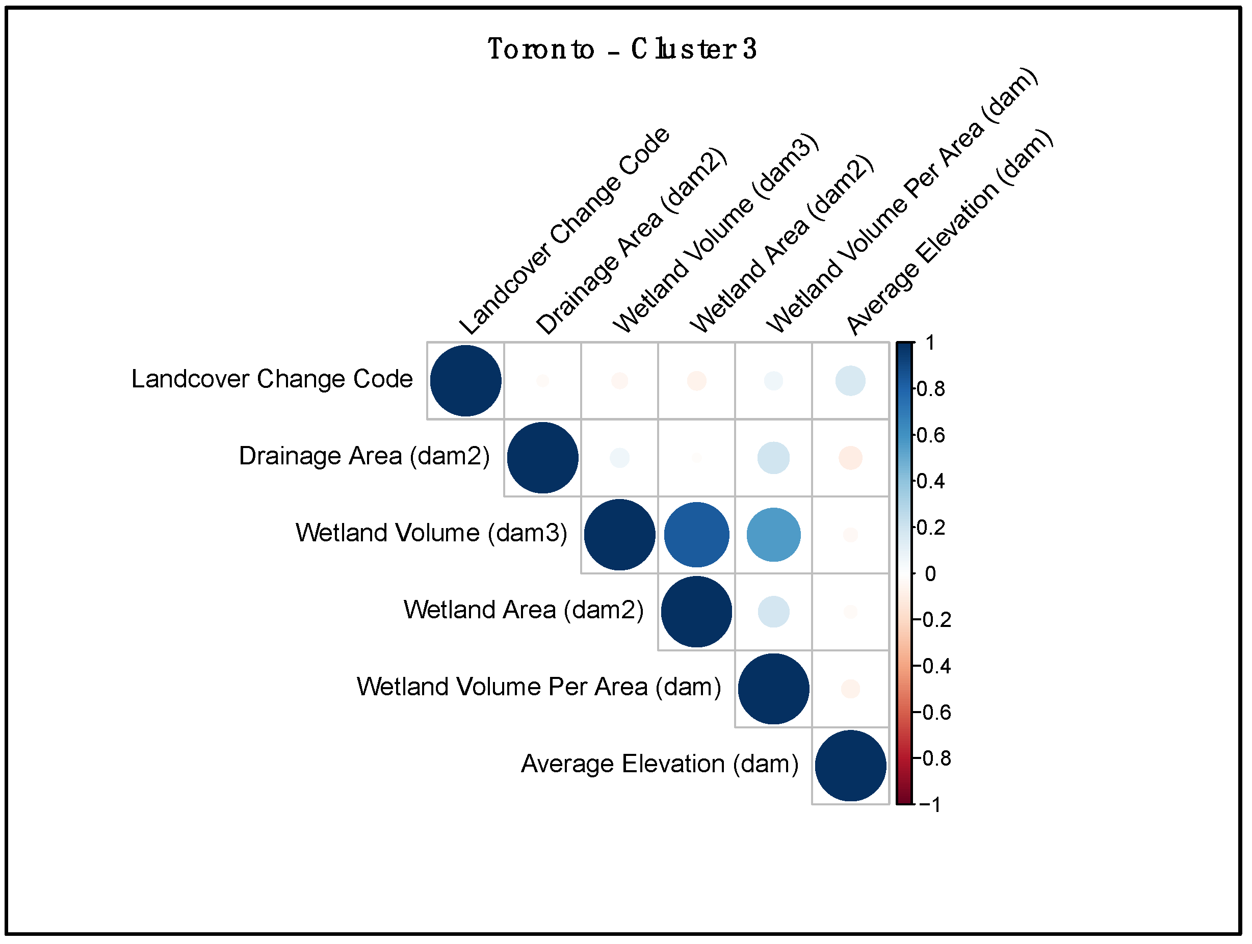
The SOM analysis results have grouped the areas classified as wetlands in 2000 (Toronto) and 2001 (Chicago) into clusters based on their average elevation, drainage area, water storage volume per area, and intensity of landcover change between 2000 and 2015 (Toronto) and 2001–2016 (Chicago). The subsequent correlation matrices have shown the level of correlation between the variables outlined above as well as the wetland area and wetland volume. Urban wetlands provide several important ecosystem services, and the results of this analysis offer a new perspective on changing urban landscapes and urban wetland ecosystem services in Toronto and Chicago. Additionally, these results allow for insight to where more intensive landcover change is correlated with wetland areas capable of providing higher levels of flood mitigation.
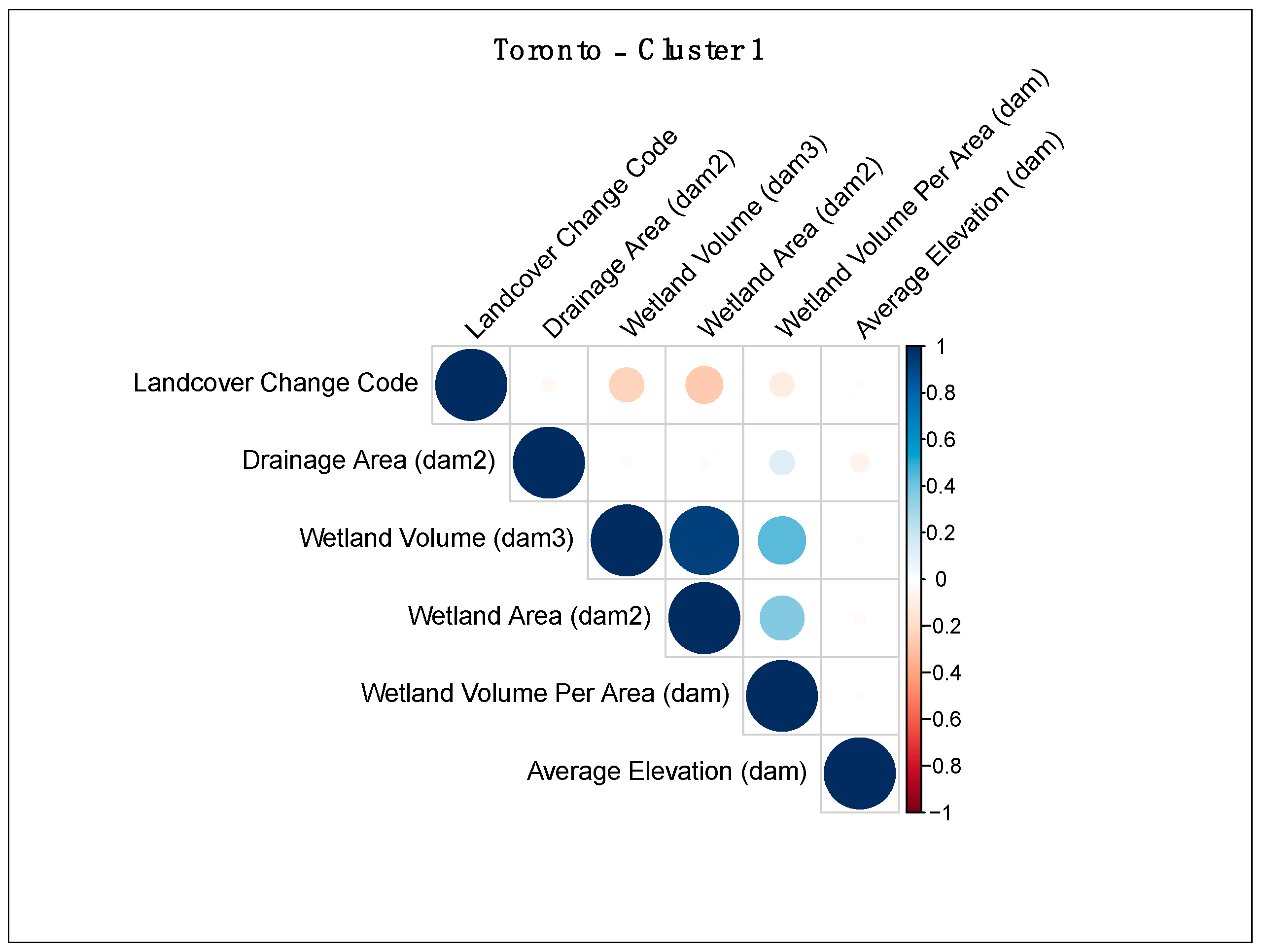
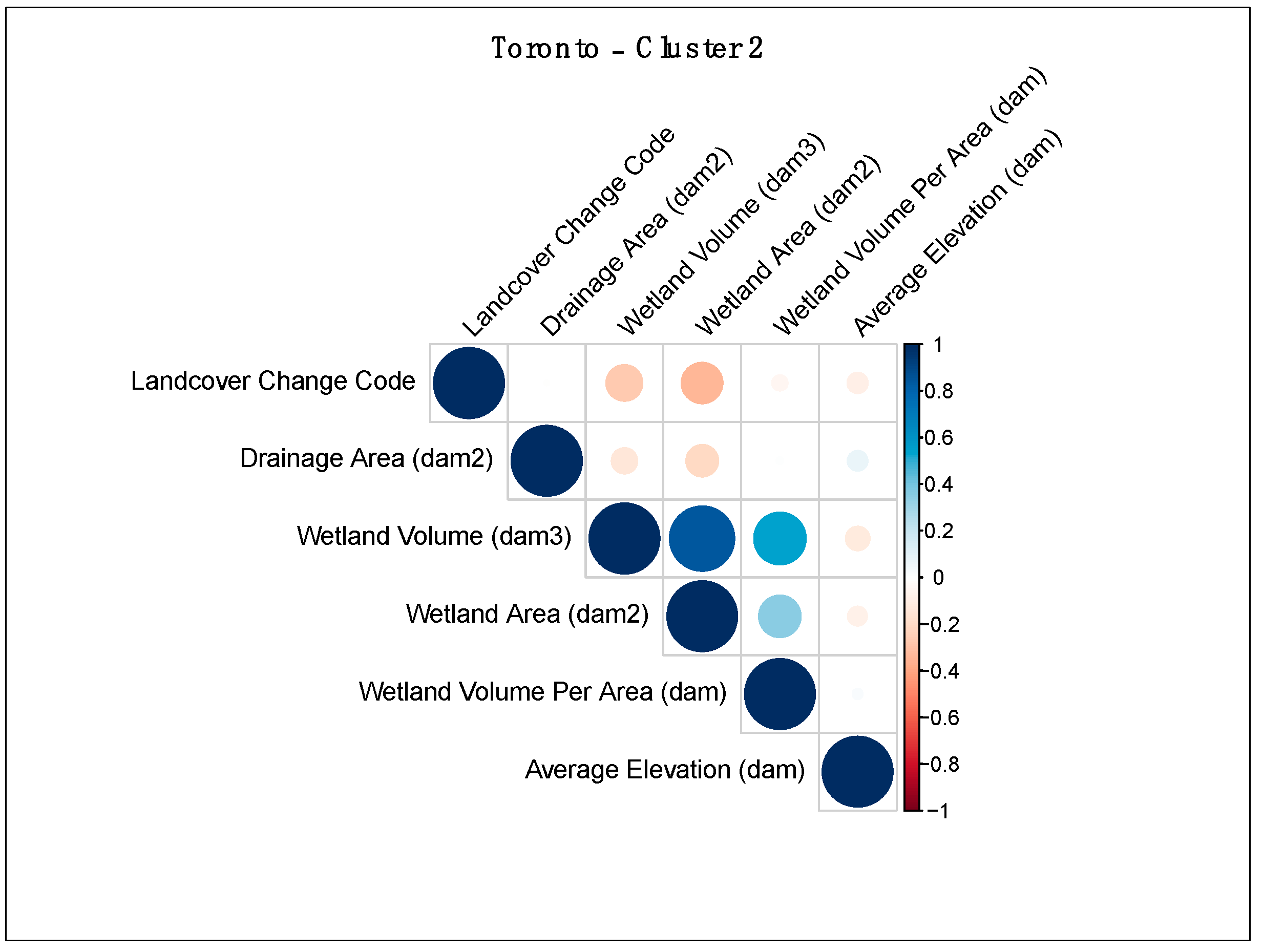
The analysis for the city of Toronto has illustrated that the wetland areas in cluster 2, cluster 4, and cluster 5 are locations where more intensive landcover change has resulted in decreases in wetland areas that have high flood mitigation potential. In cluster 2, more intense landcover change is negatively correlated with wetland area and volume, however, drainage area is also negatively correlated with wetland area and volume. This indicates that although more intense landcover change is associated with smaller wetland areas, these wetland areas tend to have larger drainage areas (i.e., a greater amount of water flowing into them during rain and snow-melting events). In cluster 4, more intense landcover change is negatively correlated with wetland area, volume, and elevation; however, it is positively correlated with drainage area. This indicates that, again, more intense landcover change is associated with smaller wetland areas at low elevations, which tend to have larger drainage areas. These correlations in cluster 4 are stronger compared to the correlations between landcover change and wetland characteristics in the other clusters. In cluster 5, more intense landcover change is negatively correlated with wetland area and volume; however, there is a positive correlation between more intense landcover and wetland volume per area. This indicates that although more intense landcover change is associated with smaller wetland areas, these wetland areas have a stable water storage capacity per area. The wetland areas included in cluster 2, cluster, 4 and cluster 5 are almost entirely situated along major waterways in Toronto. This feature increases their flood mitigation potential as wetland loss near stream networks is associated with increased stream peak flow and cumulative flow [32]. Clusters 2 and 5, in particular, have several wetland areas that are located further away from the river mouths. These wetland areas are important to highlight for potential restoration and protection, as evidence suggests that wetlands located further upstream provide greater flood reduction [33]. Broadly, in the city of Toronto analysis more intense landcover change tends to be correlated with small shallow wetlands, and the ecosystem service value of small wetlands should not go unrecognized. The cumulative services of many small wetlands can be highly effective at reducing the overland flow of water, particularly if the wetlands are situated along hydrological pathways and low elevations, and have higher evapotranspiration rates [34,35].
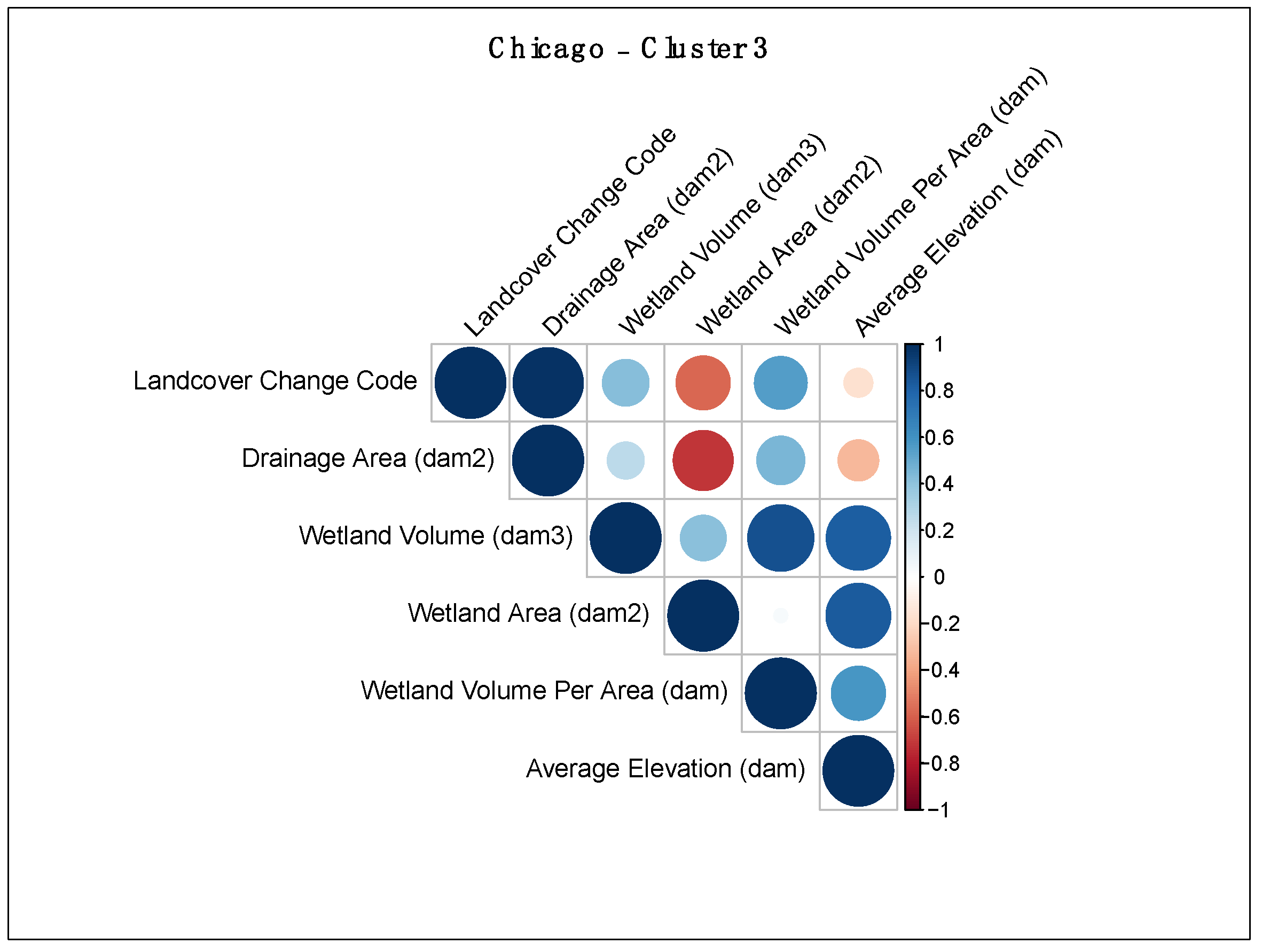
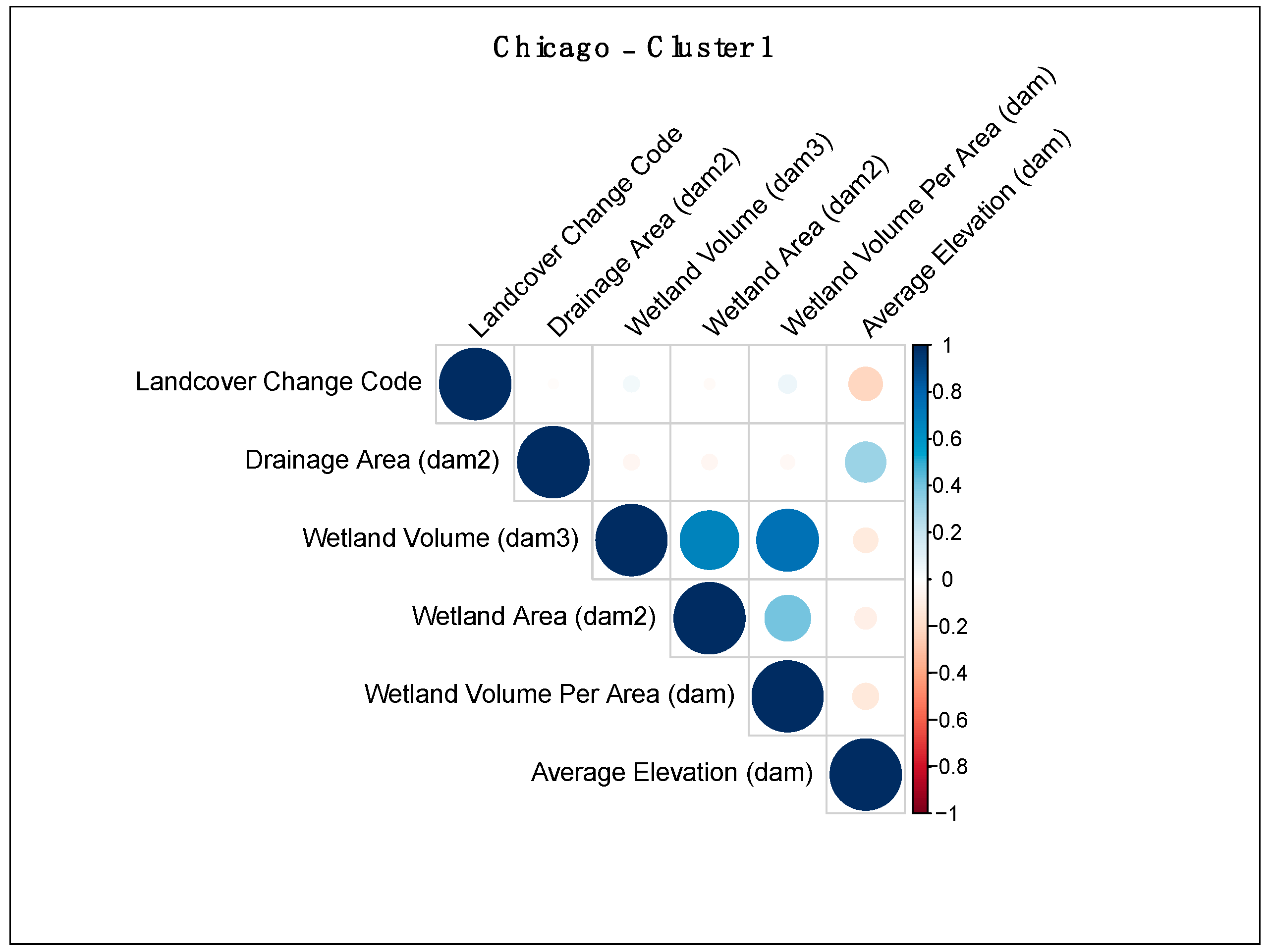
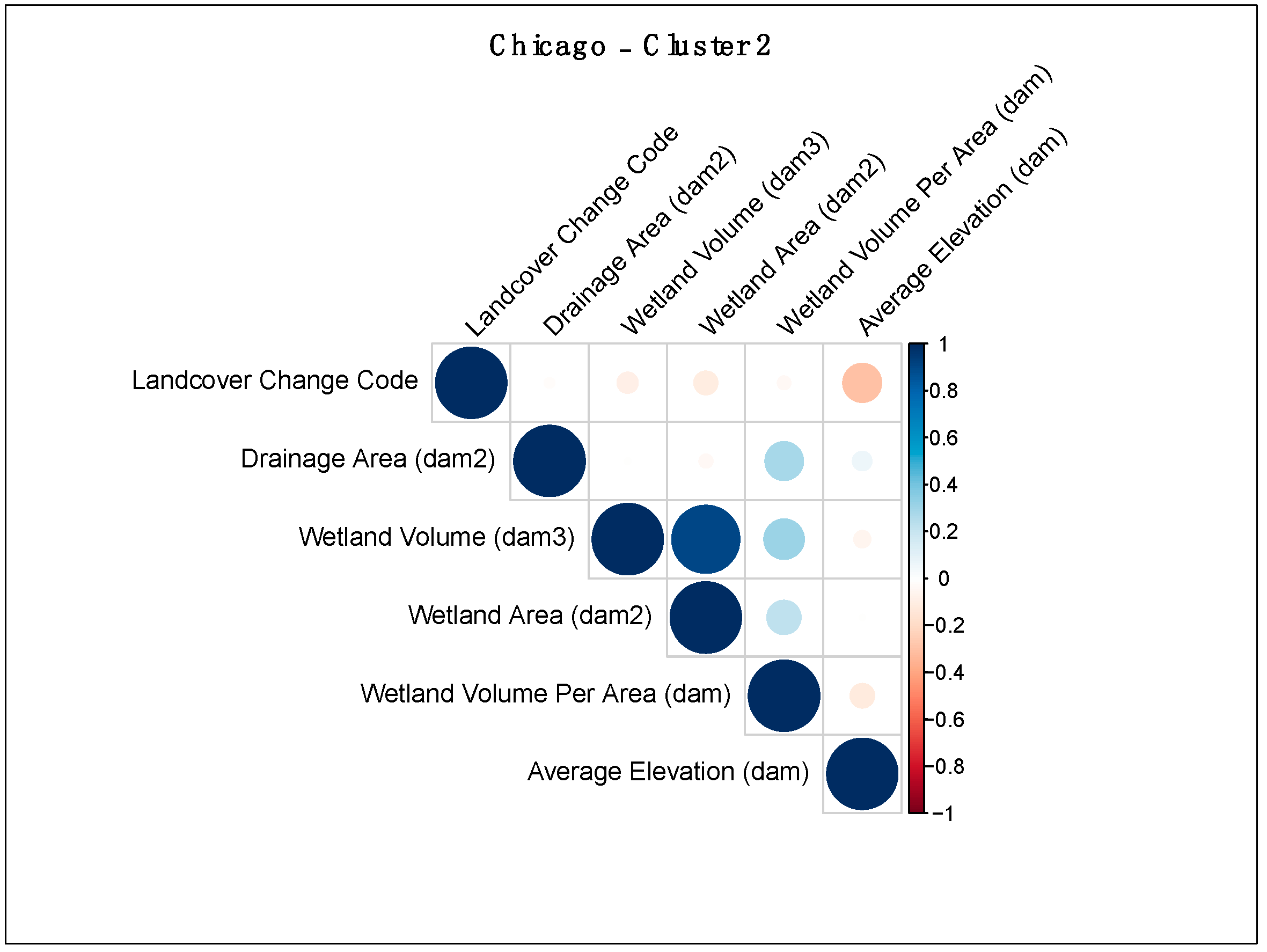
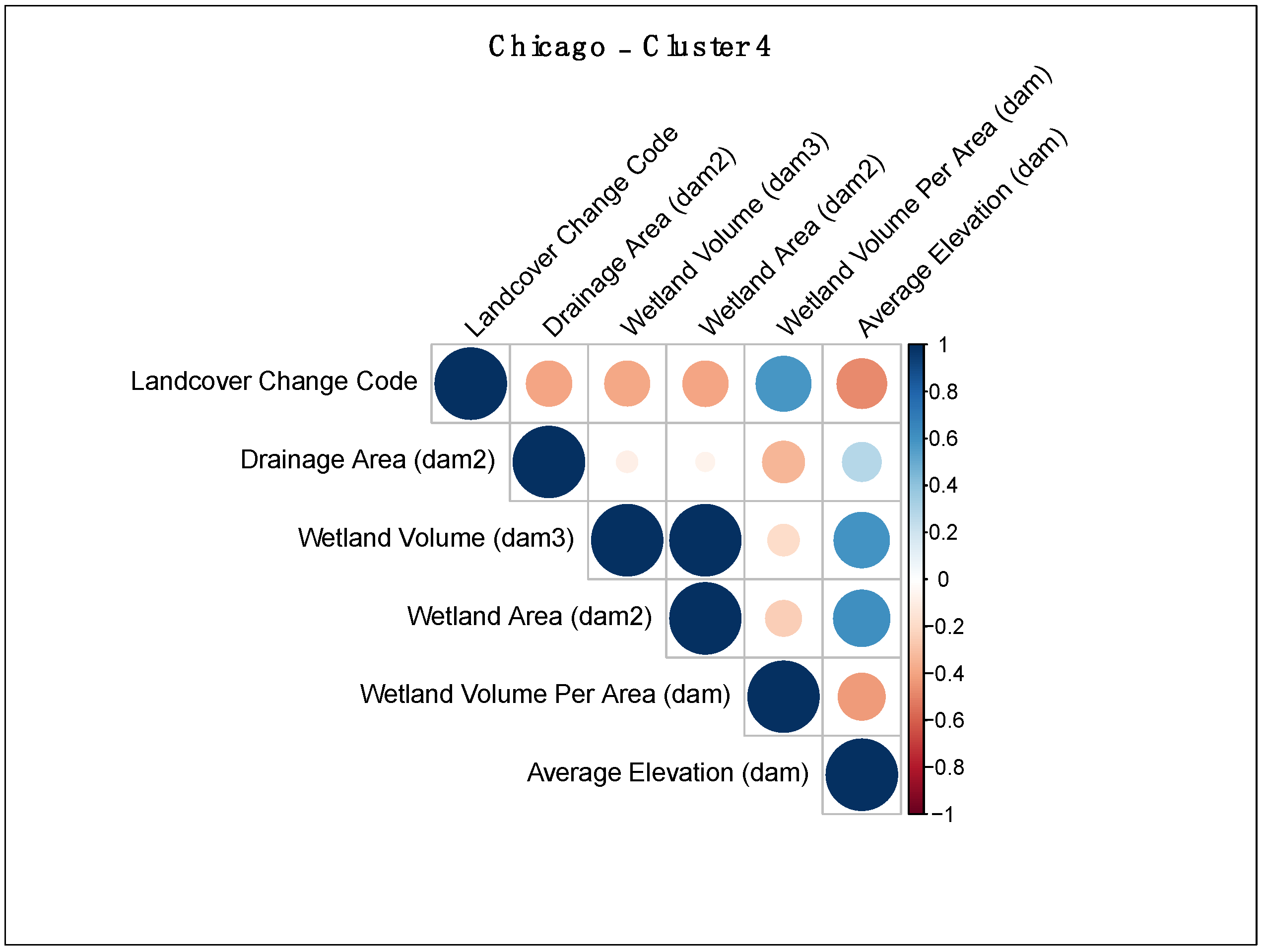
The analysis for the city of Chicago has illustrated that the wetland areas in cluster 3 and cluster 4 are locations where more intensive landcover change is correlated with wetland areas that have high flood mitigation potential. In cluster 3, more intense landcover change is negatively correlated with wetland area; however, it is positively correlated with wetland volume, wetland volume per area, and drainage area. This indicates that although more intense landcover change is associated with small wetland areas, these wetland areas have high water storage capacity per area and a greater amount of water flowing into them during rain and snow-melting events. The depth and high water storage capacity per area of the wetlands in cluster 3 is important to highlight because although wetland depth doesn’t alter storm water runoff flow significantly during small floods, during larger floods deeper wetlands are able to more greatly reduce the peak flow of storm water runoff compared to shallow wetlands [36]. In cluster 4, more intense landcover change is negatively correlated with wetland area, wetland volume, drainage area, and elevation; however, it is positively correlated with wetland volume per area. This indicates that although more intense landcover change is associated with smaller wetland areas at low elevations, these wetland areas tend to have a higher water storage capacity per area. Broadly, in the city of Chicago, more intense landcover change tends to be correlated with spatially small wetlands that have a relatively high water-storage capacity per area and are located at lower elevations. The ecosystem service value of small wetlands has already been highlighted in this discussion, and the value of Chicago’s wetland areas in cluster 3 and cluster 4 can be further displayed by their proximity to the Des Plaines River. The Des Plaines River runs through Chicago in the northwest corner of the city, and this is where all the wetland areas in cluster 3, and a large portion of the wetland areas in cluster 4, are located. Each year, flooding of the Des Plaines River costs property owners and local governments USD 20 million. This cost of flooding is linked to wetland loss, and evidence suggests that the presence of these lost wetlands would mitigate the impacts of annual floods [37].
In both cities, the smallest clusters represent wetland areas, where (1) increased landcover change is correlated with high flood mitigation potential, and (2) wetland restoration and protection would be beneficial in terms of increasing flood mitigation potential. In the city of Toronto, this is cluster 4, which includes wetlands located near the mouth of the Humber River, along Rouge River, and Highland Creek watercourses, and a single, isolated wetland area removed from the urban watercourses, located near the city’s centre. In the city of Chicago, this is cluster 3, which includes a small cluster of deep wetlands located along the shore of the Des Plaines River.
The impacts of climate change, in tandem with continued urban development, are projected to increase the severity of urban flooding events. Climate change will lead to more severe and frequent rain events and urban development will increase the aerial extent of impervious surfaces in urban areas. An important solution to this issue is the protection and restoration of natural wetlands as well as the construction of artificial wetlands. Increasing wetland areas has been shown to limit flood risk by improving groundwater infiltration, altering water delivery routes to streams, and lowering overland water transport rates [38]. Wetland areas have the potential to limit the impacts of increasing flooding events associated with climate change. However, freshwater wetlands are also particularly vulnerable to the impacts of climate change [39,40]. It is therefore recommended that the wetland areas included in clusters 2, 4 and 5, and clusters 3 and 4 for Toronto and Chicago, respectively, be actively considered for protection and restoration.
The authors recognize that there are some limitations to this study. First, landcover classification datasets are highly important tools for ecological and landcover change research; however, there are challenges in achieving complete accuracy in the classification of regional landcover datasets [41]. The authors acknowledge that there may be some errors in the landcover datasets used in this study, particularly in the classification of spatially small wetland areas. Landcover datasets were acquired from the same source for each region to (1) reduce errors in the landcover change analysis and (2) ensure that the same methodological approaches to landcover classification were applied to the datasets used in the compared time periods. Second, wetlands are part of complex hydrological systems and there are additional wetland characteristics that can contribute to water retention capacity (e.g., vegetation and soil composition) that were not included in this study [42,43]. The authors acknowledge this limitation; however, the inclusion of vegetation and soil composition analysis within the SOM, and subsequent correlation analysis was not within the scope of this study. Rather, the goal of this study was to present a machine learning framework, which uses landcover data and high-resolution digital elevation models to explore how landcover change can influence wetlands as a flood mitigation tool.

5. Conclusions

The SOM analysis and subsequent correlation matrices in this study allow for new perspectives in understanding how the changing landcover of wetland areas may reduce or increase flood mitigation in Great Lakes urban areas. The results of this study have identified several wetlands areas, where more intensive landcover change is correlated with wetland areas capable of providing higher levels of flood mitigation. In the city of Toronto, these wetland areas, situated along the Humber River, Don River, Rouge River, and Highland Creek watercourses, are represented in cluster 2, cluster 4, and cluster 5. In the city of Chicago, these wetland areas, situated primarily along the Des Plaines River, and along the North Branch of the Chicago River and Calumet River watercourses, are represented in cluster 3 and cluster 4.
Landcover change, particularly that which leads to the reduction of pervious surfaces in urban areas, can alter water balance and increase the amount of runoff during rain and snow-melting events [44]. Wetlands in the Great Lakes region provide essential ecosystem services, including urban runoff and flood mitigation, and the protection and restoration of these wetland areas should not be neglected in urban policy development and urban management [1].

Supplementary Materials

The following are available online at https://www.mdpi.com/article/10.3390/rs13244960/s1, The SOM analysis for Toronto and Chicago were completed in R with the Kohonen package, and the correlation matrices were also completed in R with the Hmisc package (R Core Team, 2020). Code written for this study has been included as supplementary files. Map production and GIS analysis was completed in QGIS 3.14 (QGIS.org, 2019).

Author Contributions

Conceptualization, E.P. and E.V.; methodology, E.P. and E.V.; software, E.P.; validation, E.P.; formal analysis, E.P.; investigation, E.P.; resources, E.P.; data curation, E.P.; writing—original draft preparation, E.P.; writing—review and editing, E.P. and E.V.; visualization, E.P.; supervision, E.V.; project administration, E.P. and E.V.; funding acquisition, not applicable. All authors have read and agreed to the published version of the manuscript.

Funding

This research received no external funding.

Institutional Review Board Statement

Not applicable.

Informed Consent Statement

Not applicable.

Data Availability Statement

The Southern Ontario Land Resource Information System (2000–2002) v1.1 dataset is produced by the Ontario Ministry of Natural Resources and Forestry and distributed by Ontario GeoHub; the dataset can be retrieved from https://ws.gisetl.lrc.gov.on.ca/fmedatadownload/Packages/SOLRIS_2000-2002_v1_1.zip (accessed on 6 July 2021). The Southern Ontario Land Resource Information System (SOLRIS) 3.0 dataset is produced by the Ontario Ministry of Natural Resources and Forestry and distributed by Ontario GeoHub; the dataset can be retrieved from the https://ws.gisetl.lrc.gov.on.ca/fmedatadownload/Packages/SOLRIS_Version_3_0.zip (accessed on 6 July 2021). The National Landcover Database (NLCD) 2001 Land Cover (CONUS) dataset is produced by the U.S. Geological Survey (USGS), in partnership with several federal agencies, and is distributed by the Multi-Resolution Land Characteristics Consortium. The dataset can be retrieved from https://www.mrlc.gov/data/nlcd-2001-land-cover-conus (accessed on 15 July 2021). The National Landcover Database (NLCD) 2016 Land Cover (CONUS) dataset is produced by the U.S. Geological Survey (USGS), in partnership with several federal agencies, and is distributed by the Multi-Resolution Land Characteristics Consortium. The dataset can be retrieved from https://www.mrlc.gov/data/nlcd-2016-land-cover-conus (accessed on 15 July 2021). The Greater Toronto Area (GTA) Digital Elevation Model 2002 dataset is produced by the Ontario Ministry of Natural Resources and Forestry and distributed by Ontario GeoHub; the dataset can be retrieved from https://geohub.lio.gov.on.ca/maps/mnrf::greater-toronto-area-gta-digital-elevation-model-2002/about (accessed on 20 July 2021). The Chicago 10m resolution Digital Elevation Model (DEM) dataset is produced and distributed by the U.S. Geological Survey (USGS). This dataset, distributed as multiple GeoTiff images, can be retrieved from https://prd-tnm.s3.amazonaws.com/StagedProducts/Elevation/13/TIFF/n42w088/USGS_13_n42w088_20210617.tif and https://prd-tnm.s3.amazonaws.com/StagedProducts/Elevation/13/TIFF/n43w088/USGS_13_n43w088.tif (accessed on 6 August 2021).

Conflicts of Interest

The authors declare no conflict of interest.

References

  1. Sierszen, M.E.; Morrice, J.A.; Trebitz, A.S.; Hoffman, J.C. A review of selected ecosystem services provided by coastal wetlands of the Laurentian Great Lakes. Aquat. Ecosyst. Health Manag. 2012, 15, 92–106. [Google Scholar] [CrossRef]
  2. Mao, D.G.; Wang, Z.; Wu, J.; Wu, B.; Zeng, Y.; Song, K.; Yi, K.; Luo, L. China’s Wetlands Loss due to Urban Expansion. Land Degrad. Dev. 2018, 29, 2644–2657. [Google Scholar] [CrossRef]
  3. Bullock, A.; Acreman, M. The Role of Wetlands in the Hydrological Cycle. Hydrol. Earth Syst. Sci. Discuss. 2003, 7, 358–389. [Google Scholar] [CrossRef] [Green Version]
  4. Lane, C.R.; D’Amico, E. Calculating the Ecosystem Service of Water Storage in Isolated Wetlands using LiDAR in North Central Florida, USA. Wetlands 2010, 30, 967–977. [Google Scholar] [CrossRef]
  5. Kingsford, R.T.; Basset, A.; Jackson, L. Wetlands: Conservations Poor Cousins. Aquat. Conserv. 2016, 26, 892–916. [Google Scholar] [CrossRef] [Green Version]
  6. Mitsch, W.J.; Gosselink, J.G. The Value of Wetlands: Importance of Scale and Landscape Setting. Ecol. Econ. 2000, 35, 25–33. [Google Scholar] [CrossRef]
  7. Croft-White, M.V.; Cvetkovic, M.; Rokitnicki-Wojcik, D.; Midwood, J.D.; Grabas, G.P. A shoreline divided: Twelve-year water quality and landcover trends in Lake Ontario Coastal Wetlands. J. Great Lakes Res. 2017, 43, 1005–1015. [Google Scholar] [CrossRef]
  8. Kovalenko, K.E.; Brady, V.J.; Brown, N.T.; Ciborowski, J.J.H.; Danz, N.P.; Gathman, J.P.; Host, G.E.; Howe, R.W.; Johnson, L.B.; Niemi, G.J.; et al. Congruence of community thresholds in response to anthropogenic stress in Great Lakes coastal wetlands. Freshw. Sci. 2014, 33, 958–971. [Google Scholar] [CrossRef] [Green Version]
  9. Bradford, A. Averting degradation of southern Ontario wetlands due to hydrologic alterations associated with development. Can. Water Resour. J. 2016, 41, 543–553. [Google Scholar] [CrossRef]
  10. Vaz, E.; Arsanjani, J.J. Predicting Urban Growth of the Greater Toronto Area—Coupling a Markov Cellular Automata with Document Meta-Analysis. J. Environ. Inform. 2015, 25, 71–80. [Google Scholar] [CrossRef]
  11. Pasterski, M.J.; Bellagamba, A.; Chancellor, S.; Cunje, A.; Dodd, E.; Gefeke, K.; Hsieh, S.; Schassburger, A.; Smith, A.; Tucker, W.; et al. Aquatic landscape change, expirations, and introductions in the Chicago Region. Urban Ecosyst. 2020, 23, 1277–1288. [Google Scholar] [CrossRef]
  12. Greb, S.F.; DiMichele, W.A.; Gastaldo, R.A. Evolution and importance of wetlands in earth history. Geol. Soc. Am. Spec. Pap. 2006, 399, 1–40. [Google Scholar] [CrossRef] [Green Version]
  13. Evenson, G.R.; Golden, H.E.; Lane, C.R.; McLaughlin, D.L.; D’Amico, E. Depressional wetlands affect watershed hydrological, biogeochemical, and ecological functions. Ecol. Appl. 2018, 28, 353–366. [Google Scholar] [CrossRef] [PubMed]
  14. Vaz, E. Managing Urban Coastal Areas Through Landscape Metrics: An Assessment of Mumbai’s Mangrove System. Ocean Coastal Manag. 2014, 98, 27–37. [Google Scholar] [CrossRef]
  15. Bousquin, J.; Hychka, K. A Geospatial Assessment of Flood Vulnerability Reduction by Freshwater Wetlands–A Benefit Indicators Approach. Front. Environ. Sci. 2019, 7, 1–54. [Google Scholar] [CrossRef] [Green Version]
  16. Bartolai, A.M.; He, L.; Hurst, A.E.; Mortsch, L.; Paehlke, R.; Scavia, D. Climate change as a driver of change in the Great Lakes St. Lawrence River Basin. J. Great Lakes Res. 2015, 41, 45–58. [Google Scholar] [CrossRef]
  17. Armenakis, C.; Nirupama, N. Flood Risk Mapping for the City of Toronto. Procedia Econ. 2014, 18, 320–326. [Google Scholar] [CrossRef] [Green Version]
  18. Soulis, E.D.; Sarhadi, A.; Tinel, M.; Suthar, M. Extreme Precipitation Time Trends in Ontario, 1960–2010. Hydrol. Process 2016, 30, 4090–4100. [Google Scholar] [CrossRef]
  19. Illinois Department of Natural Resources. Available online: https://www2.illinois.gov/dnr/WaterResources/Pages/HistoryofFloodControlDrainageinNortheasternIllinois.aspx (accessed on 23 September 2021).
  20. Chon, T.-S. Self-Organizing Maps applied to ecological sciences. Ecol. Inform. 2011, 6, 50–61. [Google Scholar] [CrossRef]
  21. Lee, B.-H.; Scholz, M. Application of the self-organizing map (SOM) to assess the heavy metal removal performance in experimental constructed wetlands. Water Res. 2006, 40, 3367–3374. [Google Scholar] [CrossRef]
  22. Zhang, L.; Scholz, M.; Mustafa, A.; Harrington, R. Application of the self-organizing map as a prediction tool for an integrated constructed wetland agroecosystem treating agricultural runoff. Bioresour. Technol. 2009, 100, 559–565. [Google Scholar] [CrossRef]
  23. Li, Z.; Bagan, H.; Yamagata, Y. Analysis of spatiotemporal land cover changes in Inner Mongolia using self-organizing map neural network and grid cells method. Sci. Total Environ. 2018, 636, 1180–1191. [Google Scholar] [CrossRef]
  24. Snedden, G.A. Patterning emergent marsh vegetation assemblages in coastal Louisiana, USA, with unsupervised artificial neural networks. Appl. Veg. Sci. 2019, 22, 213–229. [Google Scholar] [CrossRef]
  25. Vaz, E.; Zhao, Y.; Cusimano, M. Urban Habitats and the Injury Landscape. Habitat Int. 2016, 56, 52–62. [Google Scholar] [CrossRef]
  26. Vaz, E.; Bação, F.; Damásio, B.; Haynes, M.; Penfound, E. Machine learning for analysis of wealth in cities: A spatial-empirical examination of wealth in Toronto. Habitat Int. 2021, 108, 102319. [Google Scholar] [CrossRef]
  27. Burn, K.; Home, G. Environment classification using Kohonen self-organizing maps. Expert Syst. 2008, 25, 98–114. [Google Scholar] [CrossRef]
  28. Kohonon, T. Essentials of the self-organizing map. Neural Netw. 2013, 37, 52–65. [Google Scholar] [CrossRef] [PubMed]
  29. Wu, Q.; Lane, C.R. Delineating wetland catchments and modeling hydrologic connectivity using LiDAR data and aerial imagery. Hydrol Earth Syst. Sci. 2017, 2, 3579–3595. [Google Scholar] [CrossRef] [Green Version]
  30. QGIS. Available online: https://www.qgis.org (accessed on 19 June 2020).
  31. The R Project for Statistical Computing. Available online: https://www.R-project.org/ (accessed on 23 June 2020).
  32. Ameli, A.A.; Creed, I.F. Does Wetland Location Matter When Managing Wetlands for Watershed—Scale Flood and Drought Resilience? J. Am. Water Resour. Assoc. 2019, 55, 529–542. [Google Scholar] [CrossRef]
  33. Tang, Y.; Leon, A.S.; Kavvas, M.L. Impact of Size and Location of Wetlands on Watershed Scale Flood Control. Water Resour. Manag. 2020, 34, 1693–1707. [Google Scholar] [CrossRef]
  34. Potter, K.W. Estimating Potential Reduction Flood Benefits of Restored Wetlands. Water Resour. 1994, 97, 34–38. [Google Scholar]
  35. Blackwell, M.S.A.; Pilgrim, E.S. Ecosystem services delivered by small-scale wetlands. Hydrol. Sci. J. 2011, 56, 1467–1484. [Google Scholar] [CrossRef] [Green Version]
  36. Javaheri, A.; Babbar-Sebens, M. On comparison of peak flow reductions, flood inundation maps, and velocity maps in evaluating effects of restored wetlands on channel flooding. Ecol. Eng. 2014, 17, 132–145. [Google Scholar] [CrossRef]
  37. Heneghan, L.; Mulvaney, C.; Ross, K.; Stewart, S.; Umek, L.; Watkins, C.; Waki, A.; Westphal, L.M.; Wise, D.H. Local Assessment of Chicago: From Wild Chicago to Chicago Wilderness—Chicago’s Ecological Setting and Recent Efforts to Protect and Restore Nature in the Region. In Urbanization, Biodiversity and Ecosystem Services: Challenges and Opportunities, A Global Assessment; Elmqvist, T., Fragkias, M., Goodness, J., Güneralp, B., Marcotullio, P.J., McDonald, R.I., Parnell, S., Schewenius, M., Sendstad, M., Seto, K.C., et al., Eds.; Springer: Dordrecht, The Netherlands, 2013; pp. 337–354. [Google Scholar] [CrossRef] [Green Version]
  38. Waterloo University—Wetlands Report. Available online: https://www.taywatershed.ca/documents/When-the-Big-Storms-Hit.pdf (accessed on 14 October 2021).
  39. Kundzewicz, Z.W.; Mata, L.J.; Arnell, N.W.; Döll, P.; Jimenez, B.; Miller, K.; Oki, T.; Sen, Z.; Shiklomanov, I. The implications of projected climate change for freshwater resources and their management. Hydrol. Sci. J. 2008, 53, 3–10. [Google Scholar] [CrossRef]
  40. Johnson, W.C.; Werner, B.; Guntenspergen, G.R.; Voldseth, R.A.; Millett, B.; Naugle, D.E.; Tulbure, M.; Carroll, R.W.H.; Tracy, J.; Olawsky, C. Prairie Wetland Complexes as Landscape Functional Units in a Changing Climate. Bioscience 2010, 60, 128–140. [Google Scholar] [CrossRef] [Green Version]
  41. Estes, L.D.; McRitchie, D.; Choi, J.; Debats, S.; Evans, T.; Guthe, W.; Luo, D.; Ragazzo, G.; Zempleni, R.; Caylor, K.K. A platform for crowdsourcing the creation of representative, accurate landcover maps. Environ. Model. Softw. 2015, 80, 41–53. [Google Scholar] [CrossRef]
  42. Jiang, M.; Lu, X.-g.; Xu, L.-s.; Chu, L.-j.; Tong, S. Flood mitigation benefit of wetland soil—A case study in Momoge National Nature Reserve in China. Ecol. Econ. 2006, 61, 217–223. [Google Scholar] [CrossRef]
  43. Scholz, M. Wetlands and Sustainable Drainage. In Wetland Systems—Storm Water Management Control; Springer: London, UK, 2011; pp. 149–216. [Google Scholar] [CrossRef]
  44. Rizzo, A.; Bresciani, R.; Masi, F.; Boano, F.; Revelli, R.; Ridolfi, L. Flood reduction as an ecosystem service of constructed wetlands for combined sewer overflow. J. Hydrol. 2018, 560, 150–159. [Google Scholar] [CrossRef]
Figure 1. Toronto SOM clusters.
Remotesensing 13 04960 g001
Figure 2. Toronto cluster 1 correlation matrix.
Remotesensing 13 04960 g002
Figure 3. Toronto cluster 2 correlation matrix.
Remotesensing 13 04960 g003
Figure 4. Toronto cluster 3 correlation matrix.
Remotesensing 13 04960 g004
Figure 5. Toronto cluster 4 correlation matrix.
Remotesensing 13 04960 g005
Figure 6. Toronto cluster 5 correlation matrix.
Remotesensing 13 04960 g006
Figure 7. Toronto wetland SOM clusters.
Remotesensing 13 04960 g007
Figure 8. Chicago SOM clusters.
Remotesensing 13 04960 g008
Figure 9. Chicago cluster 1 correlation matrix.
Remotesensing 13 04960 g009
Figure 10. Chicago cluster 2 correlation matrix.
Remotesensing 13 04960 g010
Figure 11. Chicago cluster 3 correlation matrix.
Remotesensing 13 04960 g011
Figure 12. Chicago cluster 4 correlation matrix.
Remotesensing 13 04960 g012
Figure 13. Chicago wetland SOM clusters.
Remotesensing 13 04960 g013
Table 1. Toronto landcover change ranking system.
Landcover Change LabelLandcover Change (Ranking) Code
Treed Swamp1
Thicket Swamp1
Marsh1
Open Water2
Undifferentiated2
Forest3
Coniferous Forest3
Mixed Forest3
Deciduous Forest3
Hedge Rows3
Tilled3
Built Up Area—Pervious4
Transportation5
Built Up Area—Impervious5
Table 2. Chicago landcover change ranking system.
Landcover Change LabelLandcover Change (Ranking) Code
Wetland1
Open Water2
Mixed Forest3
Grassland/Herbaceous3
Barren Land4
Developed—Open Space4
Developed—Low Intensity4
Developed—Medium Intensity5
Developed—High Intensity5
Publisher’s Note: MDPI stays neutral with regard to jurisdictional claims in published maps and institutional affiliations.

