1. Introduction
The technological development of air and spaceborne sensors and the increasing number of remote sensing missions have allowed the continuous collection of large amounts of high quality remotely sensed data. These data are often composed of multi- and hyperspectral satellite imagery, essential for numerous applications, such as Land Use/Land Cover (LULC) change detection, ecosystem management [
1], agricultural management [
2], water resource management [
3], forest management, and urban monitoring [
4]. Despite LULC maps being essential for most of these applications, their production is still a challenging task [
5,
6]. They can be updated using one of the following strategies:
Photo-interpretation. This approach consists of evaluating a patch’s LULC class by a human operator based on orthophoto and satellite image interpretation [
7]. This method guarantees a decent level of accuracy, as it is dependent on the interpreter’s expertise and human error. Typically, it is an expensive, time-consuming task that requires the expertise of a photo-interpreter. This task is also frequently applied to obtain ground-truth labels for training and/or validating Machine Learning (ML) algorithms for related tasks [
8,
9].
Automated mapping. This approach is based on the usage of a ML method or a combination of methods in order to obtain an updated LULC map. The development of a reliable automated method is still a challenge among the ML and remote sensing community, since the effectiveness of existing methods varies across applications and geographical areas [
5]. Typically, this method requires the existence of ground-truth data, which are frequently outdated or nonexistent for the required time frame [
1]. On the other hand, employing a ML method provides readily available and relatively inexpensive LULC maps. The increasing quality of state-of-the-art classification methods has motivated the application and adaptation of these methods in this domain [
10].
Hybrid approaches. These approaches employ photo-interpreted data to augment the training dataset and improve the quality of automated mapping [
11]. They attempt to accelerate the photo-interpretation process by selecting a smaller sample of the study area to be interpreted. The goal is to minimize the inaccuracies found in the LULC map by supplying high-quality ground-truth data to the automated method. The final (photo-interpreted) dataset consists of only the most informative samples, i.e., patches that are typically difficult to classify for a traditional automated mapping method [
12].
The latter method is best known as AL. It is especially useful whenever there is a shortage or even absence of ground-truth data and/or the mapping region does not contain updated LULC maps [
13]. In a context of limited sample-collection budget, the collection of the most informative samples capable of optimally increasing the classification accuracy of a LULC map is of particular interest [
13]. AL attempts to minimize the human–computer interaction involved in photo-interpretation by selecting the data points to include in the annotation process. These data points are selected based on an uncertainty measure and represent the points close to the decision borders. Afterwards, they are passed on for photo-interpretation and added to the training dataset, while the points with the lowest uncertainty values are ignored for photo-interpretation and classification. This process is repeated until a convergence criterion is reached [
14].
The relevant work developed within AL is described in detail in
Section 2. This paper attempts to address some of the challenges found in AL, mainly inherited from automated and photo-interpreted mapping: mapping inaccuracies and time consuming human–computer interactions. These challenges have different sources:
Human error. The involvement of photo-interpreters in the data labeling step carries an additional risk to the creation of LULC patches. The minimum mapping unit being considered and the quality of the orthophotos and satellite images being used are some of the factors that may lead to the overlooking of small-area LULC patches and label-noisy training data [
15].
High-dimensional datasets. Although all the bands (i.e., features) present in multi- and hyperspectral images contain useful information for automated classification, they also introduce an increased level of complexity and redundancy in the classification step [
16]. These datasets are often prone to the Hughes phenomenon, also known as the curse of dimensionality.
Class separability. Producing an LULC map considering classes with similar spectral signatures makes them difficult to separate [
17]. A lower pixel resolution of the satellite images may also imply mixed-class pixels, which may lead to both lower class separability and higher risk of human error.
Existence of rare land cover classes. The varying morphologies of different geographical regions naturally implies an uneven distribution of land cover classes [
18]. This is particularly relevant in the context of AL since the data selection method is based on a given uncertainty measure over data points whose class label is unknown. Consequently, AL’s iterative process of data selection may disregard wrongly classified land cover areas belonging to a minority class.
Research developed in the field of AL typically focuses on the reduction of human error by minimizing the human interaction with the process through the development of more efficient classifiers and selection criteria within the generally accepted AL framework. Concurrently, the problem of rare land cover classes is rarely addressed. This is a frequent problem in the ML community, known as the Imbalanced Learning problem. This problem exists whenever there is an uneven between-class distribution in the dataset [
19]. Specifically, most classifiers are optimized and evaluated using accuracy-like metrics, which are designed to work primarily with balanced datasets. Consequently, these metrics tend to introduce a bias towards the majority class by attributing an importance to each class proportional to its relative frequency [
10]. For example, such a classifier could achieve an overall accuracy of 99% on a binary dataset where the minority class represents 1% of the overall dataset and thus still be useless. Several methods have been developed to deal with this problem. They can be categorized into three different types of approaches [
20,
21]. Cost-sensitive solutions perform changes to the cost matrix in the learning phase. Algorithmic level solutions modify specific classifiers to reinforce learning on minority classes. Resampling solutions modify the training data by removing majority samples and/or generating artificial minority samples. The latter is independent from the context and can be used alongside any classifier. Since we are interested in the introduction of artificial data generation in AL, we analyze the state of the art on resampling techniques (specifically oversampling) in
Section 3.
In this paper, we propose a novel AL framework to address two limitations commonly found in the literature: minimize human–computer interaction and reduce the class imbalance bias. This is done with the introduction of an additional component in the iterative AL procedure (the generator) that is used to generate artificial data to both balance and augment the training dataset. The introduction of this component is expected to reduce the number of iterations required until the classifier reaches a satisfactory performance.
This paper is organized as follows.
Section 1 explains the problem and its context.
Section 2 and
Section 3 describe the state of the art in AL and oversampling techniques.
Section 4 explains the proposed method.
Section 5 covers the datasets, evaluation metrics, ML classifiers, and experimental procedure.
Section 6 presents the experiment’s results and discussion.
Section 7 presents the conclusions drawn from our findings.
2. Active Learning Approaches
As the amount of unlabeled data increases, the interest and practical usefulness of AL follows that trend [
22]. AL is used as the general definition of frameworks aiming to train a learning system in multiple steps, where a new dataset is chosen and added to the training dataset each time [
11]. Typically, an AL framework is composed of the following elements [
11,
13,
23]:
Unlabeled dataset. It consists of the original data source (or a sample thereof). It is used in combination with the chooser and the selection criterion to expand the training dataset in regions where the classification uncertainty is higher. Therefore, the unlabeled dataset is used for both producing the initial training dataset by selecting a set of instances for the supervisor to annotate (discussed in point 3) and calculating the uncertainty map to augment the training dataset.
Supervisor. It is a human annotator (or team of human annotators) to whom the uncertainty map is presented. The supervisor is responsible for annotating unlabeled instances to be added to the augmented dataset. In remote sensing, the supervisor is typically a photo-interpreter, as is the case in [
24]. Some research also refers to the supervisor as the
oracle [
11,
25,
26,
27].
Initial training dataset. It is a small, labeled sample of the original data source used to initiate the first AL iteration. The size of the initial training sample normally varies between no instances at all and 10% of the unlabeled dataset [
28].
Current and expanded training dataset. It is the concatenation of the initial training dataset and the datasets labeled by the supervisor in past iterations (discussed in Point 2).
Chooser (classifier). It produces the class probabilities for each unlabeled instance.
Selection criterion. It quantifies the chooser’s uncertainty level for each instance belonging to the unlabeled dataset. It is typically based on the class probabilities assigned by the chooser. In some situations, the chooser and the selection criterion are grouped together under the concept
acquisition function [
11] or
query function [
13]. Some of the literature refers to the selection criterion by using the concept
sampling scheme [
12].
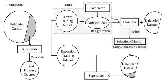
Figure 1 schematizes the steps involved in a complete AL iteration. For a better context within the remote sensing domain, the prediction output can be identified as the LULC map. This framework starts by collecting unlabeled data from the original data source. They are used to generate a random initial training sample and are labeled by the supervisor. In practical applications, the supervisor is frequently a group of photo-interpreters [
22]. The chooser is trained on the resulting dataset and is used to predict the class probabilities on the unlabeled dataset. The class probabilities are fed into a selection criterion to estimate the prediction’s uncertainty, out of which the instances with the highest uncertainty will be selected. This calculation is motivated by the absence of labels in the uncertainty dataset. Therefore, it is impossible to estimate the prediction’s accuracy in the unlabeled dataset in a real case scenario. The iteration is completed when the selected points are tagged by the supervisor and added to the training dataset (i.e., the augmented dataset).
A common challenge found in AL tasks is ensuring the consistency of AL over different initializations [
22]. There are two factors involved in this phenomenon. On the one hand, the implementation of the same method over different initializations may result in significantly different initial training samples, leading to varying accuracy curves. On the other hand, the lack of a robust selection criterion and/or classifier may also result in inconsistencies across AL experiments with different initializations. This phenomenon was observed and documented in a LULC classification context in [
29].
The classification method plays a central role in the efficacy of AL. The classifier used should be able to generalize with a relatively small training dataset. Specifically, deep learning models are used in image classification due to their capability of producing high quality predictions. However, to make such models generalizable, the training set must be large enough, making its suitability for AL applications an open challenge [
30,
31,
32]. Some studies in the remote sensing domain were developed to address this gap. In [
30,
32], the authors proposed a deep learning-based AL approach by training the same convolutional neural network incrementally across iterations and smoothening the decision boundaries of the model using the Markov random field model and a best-versus-second best labeling approach. This allows the introduction of additional data variability in the final training dataset. Wu et al. [
31] combined transfer learning, active classification and segmentation techniques for vehicle detection. By combining different techniques, they were able to produce a classification mechanism that performed well when the amount of training data is limited. However, the exploration of advanced deep learning classifiers in AL is still limited. In [
33], the authors showed that deep learning classifiers performs well on LULC classification, but are still not generalizable for different geographical regions or periods. Specifically, AL methods are still incapable of providing generalizable deep learning classifiers, which benefit from multiple advantages. The development of convolutional neural networks with both two- and three-dimensional convolutions was explored by Roy et al. [
34] who reported superior classification performance on benchmark datasets. However, many training data were used to produce the final classification map.
Selecting an efficient selection criterion is particularly important to find the instances closest to the decision border (i.e., instances difficult to classify) [
35]. Therefore, many AL related studies focus on the design of the query/acquisition function [
13].
2.1. Non-Informed Selection Criteria
Only one non-informed (i.e., random) selection criterion was found in the literature. Random sampling selects unlabeled instances without considering any external information produced by the chooser. Since the method for selecting the unlabeled instances is random, this method disregards the usage of a chooser and is comparatively worse than any other selection criterion. However, random sampling is still a powerful baseline method [
27].
2.2. Ensemble-Based Selection Criteria
Ensemble disagreement is based on the class predictions of a set of classifiers. The disagreement between all the predictions for a given instance is a common measure for uncertainty, although computationally inefficient [
11,
14]. It is calculated using the set of classifications over a single instance, given by the number of votes assigned to the most frequent class [
35]. This method was implemented successfully for complex applications such as deep active learning [
11].
Multiview [
36] consists on the training of multiple independent classifiers using different views, which correspond to the selection of subsets of features or instances in the dataset. Therefore, it can be seen as a bootstrap aggregation (bagging) ensemble disagreement method. It is represented by the maximum disagreement score out of a set of disagreements calculated for each view [
35]. A lower value for this metric means a higher classification uncertainty. Multiview-based maximum disagreement has been successfully applied to hyperspectral image classification [
37,
38].
An adapted disagreement criterion for an ensemble of
k-nearest neighbors is proposed in [
14]. This method employs a
k-nearest neighbors classifier and computes an instance’s classification uncertainty based on the neighbors’ class frequency using the maximum disagreement metric over varying values for
k. As a result, this method is comparable to computing the dominant class’ score over a weighted
k-nearest neighbors classifier. This method was also used on a multimetric active learning framework by Zhang et al. [
39].
Another relevant ensemble-based selection criterion is the binary random forest-based query model [
13]. This method employs a one-versus-one ensemble method to demonstrate an efficient data selection method using the estimated probability of each binary random forest and determining the classification uncertainty based on the probabilities closest to 0.5 (i.e., the least separable pair of classes is used to determine the uncertainty value). However, this study fails to compare the proposed method with other benchmark methods, such as random sampling.
2.3. Entropy-Based Criteria
Several contributions have focused on entropy-based querying. The application of entropy is common among active deep learning applications [
26], where the training of an ensemble of classifiers is often too expensive.
Entropy Query-by-Bagging (EQB), also defined as maximum entropy [
12], is an ensemble approach of the entropy selection criterion, originally proposed in [
40]. This strategy uses the set of predictions produced by the ensemble classifier to calculate the many entropy measurements. The estimated uncertainty measure for one instance is given by the maximum entropy within that set. EQB has been observed to be an efficient selection criterion. Specifically, Shrivastava and Pradhan [
35] applied EQB on hyperspectral remote sensing imagery using Support Vector Machines (SVM) and Extreme Learning Machines (ELM) as choosers, achieving optimal results when combining EQB with ELM. Another study successfully implemented this method on an active deep learning application [
12]. Another study improved over this method with a normalized EQB selection criterion [
41].
2.4. Other Relevant Criteria
Margin Sampling is a SVM-specific criterion, based on the distance of a given point to the SVM’s decision boundary [
35]. This method is less popular than the remaining methods because it is limited to one type of chooser (SVMs). One extension of this method is the multi-class level uncertainty [
35], calculated by subtracting the instance’s distance to the decision boundaries of the two most probable classes [
42].
The Mutual Information-based (MI) criterion selects the new training instances by maximizing the mutual information between the classifier and class labels in order to select instances from regions that are difficult to classify. Although this method is commonly used, it is frequently outperformed by the breaking ties selection criterion [
43,
44].
The breaking ties (BT) selection criterion was originally introduced by Luo et al. [
45]. It consists of the subtraction between the probabilities of the two most likely classes. Another related method is Modified Breaking Ties scheme (MBT), which aims at finding the instances containing the largest probabilities for the dominant class [
44,
46]
Another type of selection criteria identified is the loss prediction method [
25]. This method replaces the selection criterion with a predictor whose goal is to estimate the chooser’s loss for a given prediction. This allows the new classifier to estimate the prediction loss on unlabeled instances and select the ones with the highest predicted loss.
Some of the literature fails to specify the strategy employed, although inferring it is generally intuitive. For example, Ertekin et al. [
47] successfully used AL to address the imbalanced learning problem. They employed an ensemble of SVMs as the chooser, as well as an ensemble-based selection criterion. All of the research found related to this topic focuses on the improvement of AL through modifications on the selection criterion and classifiers used. None of these publications propose significant variations to the original AL framework.
3. Artificial Data Generation Approaches
The generation of artificial data is a common approach to address imbalanced learning tasks [
21], as well as improve the effectiveness of supervised learning tasks [
48]. In recent years, some sophisticated data generation approaches have been developed. However, the scope of this work is to propose the integration of a generator within the AL framework. To do this, we focus on heuristic data generation approaches, specifically, oversamplers.
Heuristic data resampling methods employ local and/or global information to generate new, relevant, non-duplicate instances. These methods are most commonly used to populate minority classes and balance the between-class distribution of a dataset. The Synthetic Minority Oversampling Technique (SMOTE) [
49] is a popular heuristic oversampling algorithm, proposed in 2002. The simplicity and effectiveness of this method contributes to its prevailing popularity. It generates a new instance through a linear interpolation of a randomly selected minority-class instance and one of its randomly selected
k-nearest neighbors. The implementation of SMOTE for LULC classification tasks has been found to improve the quality of the predictors used [
50,
51]. Despite its popularity, its drawbacks motivates the development of other oversampling methods [
52].
Geometric SMOTE (G-SMOTE) [
52] introduces a modification of the SMOTE algorithm in the data generation mechanism to produce artificial instances with higher variability. Instead of generating artificial data as a linear combination of the parent instances, it is done within a deformed, truncated hyper-spheroid. G-SMOTE generates an artificial instance
within a hyper-spheroid, formed by selecting a minority instance
and one of its nearest neighbors
, as shown in
Figure 2. The truncation and deformation parameters define the shape of the spheroid’s geometry. The method also modifies the selection strategy for the
k-nearest neighbors, accepting the generation of artificial instances using instances from different classes, as shown in
Figure 2. The modification of both selection and generation mechanisms addresses the main drawbacks found in SMOTE, the generation of both noisy data (i.e., the generation of minority class instances within majority class regions) and near-duplicate minority class instances [
52]. G-SMOTE has shown superior performance when compared with other oversampling methods for LULC classification tasks, regardless of the classifier used [
53].
4. Proposed Method
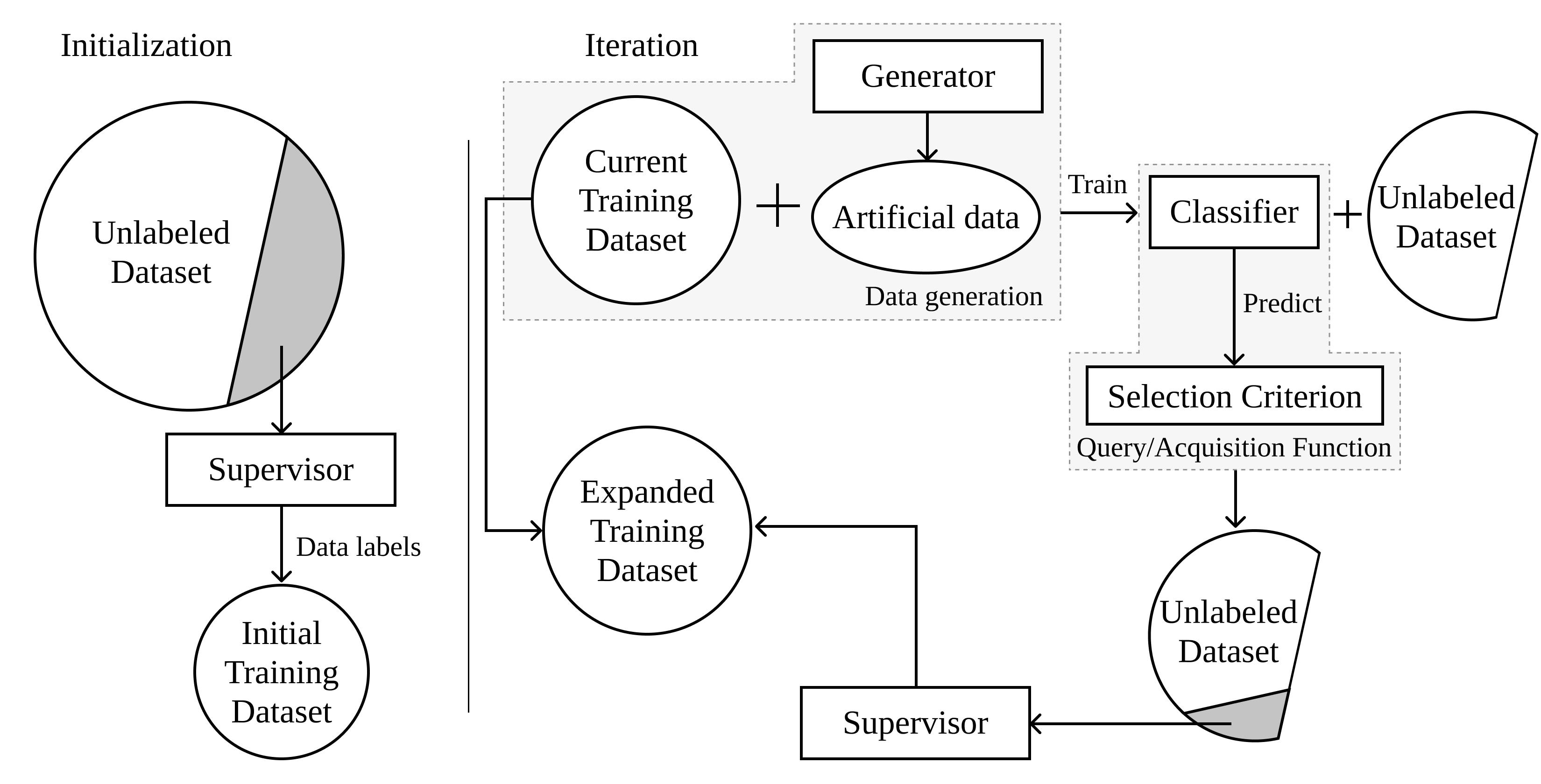
Within the literature identified, most of the work developed in the AL domain revolves around improving the quality of classification algorithms and/or selection criteria. Although these methods allow earlier convergence of the AL iterative process, the impact of these methods are only observed between iterations. Consequently, none of these contributions focus on the definition of decision borders within iterations. The method proposed in this paper modifies the AL framework by introducing an artificial data generation step within AL’s iterative process. We define this component as the generator, and it is intended to be integrated into the AL framework, as shown in
Figure 3.
This modification, by using a new source of data to augment the training set, leverages the data annotation work conducted by the human operator. The artificial data generated between iterations reduce the amount of labeled data required to reach optimal performance and lower the amount of human labor required to train a classifier to its optimal performance. This process lowers the annotation and overall training costs by translating some of the annotation cost into computational cost.
This method leverages the capability of artificial data to introduce more data variability into the augmented dataset and facilitate the chooser’s training phase with a more consistent definition of the decision boundaries at each iteration. Therefore, any algorithm capable of producing artificial data, be it agnostic or specific to the domain, can be employed. The artificial data are only used to train the classifiers involved in the process and are discarded once the training phase is completed. The remaining steps in the AL framework remain unchanged. This method addresses the limitations found in the previous sections:
The convergence of classification performance should be anticipated with the clearer definition of the decision boundaries across iterations.
Annotation cost is expected to be reduced as the need for labeled instances reduces along with the early convergence of the classification performance.
The class imbalance bias observed in typical classification tasks, as well as in AL, is mitigated by balancing the class frequencies at each iteration.
Although the performance of this method is shown within a LULC classification context, the proposed framework is independent of the domain. The high dimensionality of remotely sensed imagery makes its classification particularly challenging when the available labeled data are scarce and/or come at a high cost, being subjected to the curse of dimensionality. Consequently, it is a relevant and appropriate domain to test this method.
5. Methodology
In this section, we describe the datasets, evaluation metrics, oversampler, classifiers, software used and the procedure developed. We demonstrate the proposed method’s efficiency over seven datasets, sampled from publicly available, well-known remote sensing hyperspectral scenes frequently found in the remote sensing literature. The datasets and sampling strategy are described in
Section 5.1. On each of these datasets, we apply three different classifiers over the entire training set to estimate the optimal classification performance, the original AL framework as the baseline reference and the proposed method using G-SMOTE as a generator, described in
Section 5.2. The metrics used to estimate the performance of these algorithms are described in
Section 5.3. Finally, the experimental procedure is described in
Section 5.4.
Our methodology focuses on two objectives: (1) comparison of optimal classification performance among active learners and traditional supervised learning; and (2) comparison of classification convergence efficiency among AL frameworks.
5.1. Datasets
The datasets used were extracted from publicly available repositories containing hyperspectral images and ground truth data. Additionally, all datasets were collected using the same sampling procedure. The description of the hyperspectral scenes used in this study is provided in
Table 1. These scenes were chosen because of their popularity in the research community and their high baseline classification scores. Consequently, demonstrating an outperforming method in this context is particularly challenging and valuable.
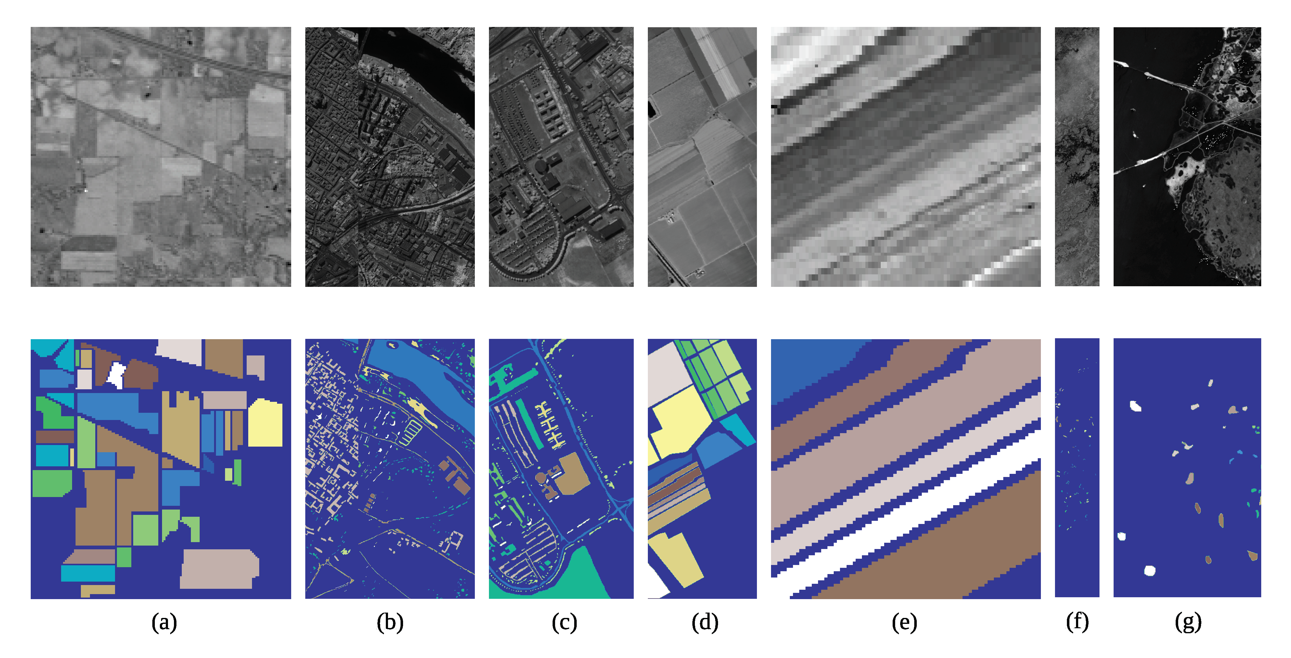
The Indian Pines scene [
54] is composed of agriculture fields in approximately two thirds of its coverage and low density built up areas and natural perennial vegetation in the remainder of its area (see
Figure 4a). The Pavia Centre and University scenes are hyperspectral, high-resolution images containing ground truth data composed of urban-related coverage (see
Figure 4b,c). The Salinas and Salinas A scenes contain at-sensor radiance data. As a subset of Salinas, the Salinas A scene contains contains the vegetable fields present in Salinas, and the latter is also composed of bare soils and vineyard fields (see
Figure 4d,e). The Botswana scene contains ground truth data composed of seasonal swamps, occasional swamps, and drier woodlands located in the distal portion of the delta (see
Figure 4f). The Kennedy Space Center scene contains a ground truth composed of both vegetation and urban-related coverage (see
Figure 4g).
The sampling strategy is similar for all datasets. The pixels without a ground truth label are first discarded. All the classes with cardinality lower than 150 are also discarded. This is done to maintain feasible Imbalance Ratios (IR) across datasets (where
). Finally, a stratified sample of 1500 instances are selected for the experiment. The resulting datasets are described in
Table 2. The motivation for this strategy is three fold: (1) reduce the datasets to a manageable size and allow the experimental procedure to be completed within a feasible time frame; (2) ensure the relative class frequencies in the scenes are preserved; and (3) ensure equivalent analyses across datasets and AL frameworks. In this context, a fixed number of instances per dataset is especially important to standardize the AL-related performance metrics.
5.2. Machine Learning Algorithms
We use two different types of ML algorithms: a data generation algorithm to form the generator and a classification algorithms to calculate the classification uncertainties in the unlabeled dataset and predict the class labels in the validation and test sets.
Although any method capable of generating artificial data can be used as a generator, the one used in this experiment is an oversampler, originally developed to deal with imbalanced learning problems. Specifically, we chose G-SMOTE, a state-of-the-art oversampler.
Three classification algorithms are used. We use different types of classifiers to test the framework’s performance under varying situations: neighbors-based, linear and ensemble models. The neighbors-based classifier chosen is
K-nearest neighbors (KNN) [
55], a logistic regression (LR) [
56] is used as the linear model, and a random forest classifier (RFC) [
57] is used as the ensemble model.
The acquisition function is completed by testing three different selection criteria. Random selection is used as a baseline selection criterion, whereas entropy and breaking ties are used due to their popularity and independence of the classifier used.
5.3. Evaluation Metrics
Since the datasets used in this experiment have an imbalanced distribution of class frequencies, metrics such as the
Overall Accuracy (OA) and
Kappa coefficient are insufficient to accurately depict classification performance [
58,
59]. Instead, metrics such as Producer’s Accuracy (or
Recall) and User’s Accuracy (or
Precision) can be used. Since they consist of ratios based on True/False Positives (TP and FP) and Negatives (TN and FN), they provide per class information regarding the classifier’s classification performance. However, in this experiment, the meaning and number of classes available in each dataset vary, making these metrics difficult to synthesize.
The performance metric
Geometric mean (G-mean) and
F-score are less sensitive to the data imbalance bias [
60,
61]. Therefore, we employ both of these scorers. G-mean consists of the geometric mean of
and
(also known as
Recall) [
61]. Both metrics are calculated in a multi-class context considering a one-versus-all approach. For multi-class problems, the
G-mean scorer is calculated as its average of per class values:
The F-score performance metric is the harmonic mean of
Precision and
Recall. The two metrics are also calculated considering a one-versus-all approach. The
F-score for the multi-class case can be calculated using its average per class values [
62]:
The comparison of classification convergence across AL frameworks and selection criteria is done using two AL-specific performance metrics. Particularly, we follow the recommendations found in [
22]. Each AL configuration is evaluated using the
Area Under the Learning Curve (AULC) performance metric. It is the sum of the classification performance values of all iterations. To facilitate the analysis of the results, we fix the range of this metric within
by dividing it by the total number of iterations (i.e., the maximum performance area).
The
Data Utilization Rate (DUR) [
63] metric consists of the ratio between the number of instances required to reach a given G-mean score threshold by an AL strategy and an equivalent baseline strategy. For easier interpretability, we simplify this metric by using the percentage of training data used by an AL strategy to reach the performance threshold, instead of presenting these values as a ratio of the baseline strategy. The DUR metric is measured at nine different performance levels, between 0.6 and 0.95 G-mean scores at a 0.05 step.
5.4. Experimental Procedure
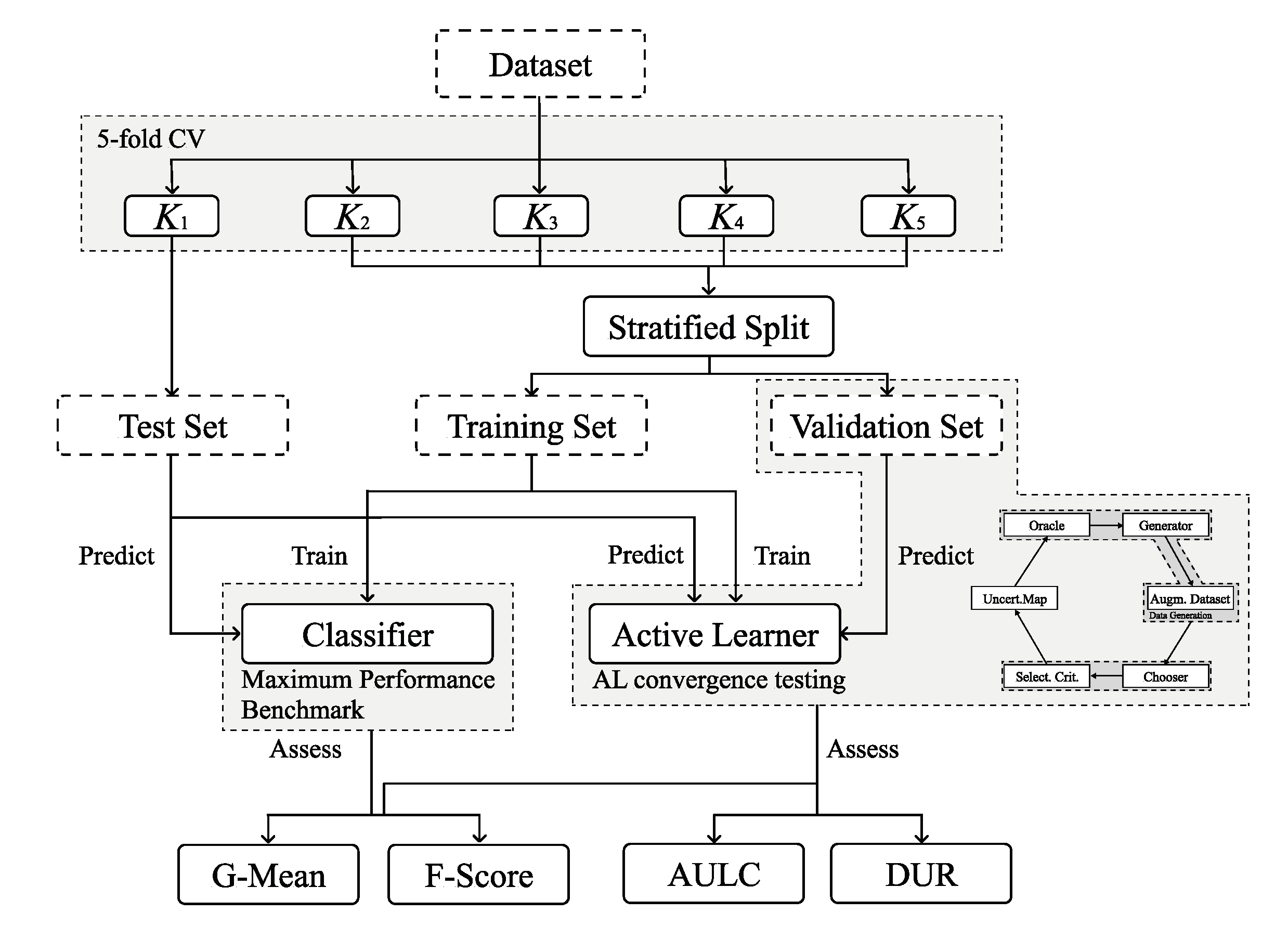
A common practice in methodological evaluations is the implementation of an offline experiment [
64]. It consists of using an existing set of labeled data as a proxy for the population of unlabeled instances. Because the dataset is already fully labeled, the supervisor’s typical annotation process involved in each iteration is done at zero cost. Each AL and classifier configuration is tested using a stratified five-fold cross validation testing scheme. For each round, the larger partition is split in a stratified fashion to form a training and validation set (containing 20% of the original partition). The validation set is used to evaluate the convergence efficiency of active learners; the chooser’s classification performance metrics and amount of data points used at each iteration are used to compute the AULC and DUR. Additionally, within the AL iterative process, the classifier with optimal performance on the validation set is evaluated using the test set. In order to further reduce possible initialization biases, this procedure is repeated three times with different initialization seeds and the results of all runs are averaged (i.e., each configuration is trained and evaluated 15 times). Finally, the maximum performance lines are calculated using the same approach. In those cases, the validation set is not used. The experimental procedure is depicted in
Figure 5.
To make the AL-specific metrics comparable among active learners, the configurations of the different frameworks must be similar. For each dataset, the number of instances is constant to facilitate the analysis of the same metrics.
In most practical AL applications, it is assumed that the number of instances in the initial training sample is too small to perform hyperparameter tuning. Consequently, in order to ensure realistic results, our experimental procedure does not include hyperparameter optimization. The predefined hyperparameters are shown in
Table 3. They are set up based on general recommendations and default settings for the classifiers and generators used.
The AL iterative process is set up with a randomly selected initial training sample with 15 initial samples. At each iteration, 15 additional samples are added to the training set. This process is stopped after 49 iterations, once 50% of the entire dataset (i.e., 78% of the training set) is added to the augmented dataset.
5.5. Software Implementation
6. Results and Discussion
The evaluation of the different AL frameworks in a multiple dataset context should not rely uniquely on the mean of the performance metrics across datasets. Demšar [
67] recommended the use of mean ranking scores, since the performance levels of the different frameworks varies according to the data it is being used on. Consequently, evaluating these performance metrics solely based on their mean values might lead to inaccurate analyses. Accordingly, the results of this experiment are analyzed using both the mean ranking and absolute scores for each model. The rank values are assigned based on the mean scores resulting from three different initializations of five-fold cross validation for each classifier and active learner. The goal of this analysis is to understand whether the proposed framework (AL with the integration of an artificial data generator) is capable of using fewer data from the original dataset while simultaneously achieving better classification results than the standard AL framework, i.e., guarantee a faster classification convergence.
6.1. Results
Table 4 shows the average rankings and standard deviations across datasets of the AULC scores for each active learner.
The mean AULC absolute scores are provided in
Table 5. These values are computed as the mean of the sum of the scores of a specific performance metric over all iterations (for an AL configuration). In other words, these values correspond to the average AULC over
.
The average DURs are shown in
Table 6. They were calculated for various G-mean scores thresholds, varying at a step of 5% between 60% and 95%. Each row shows the percentage of training data required by the different AL configurations to reach that specific G-mean score.
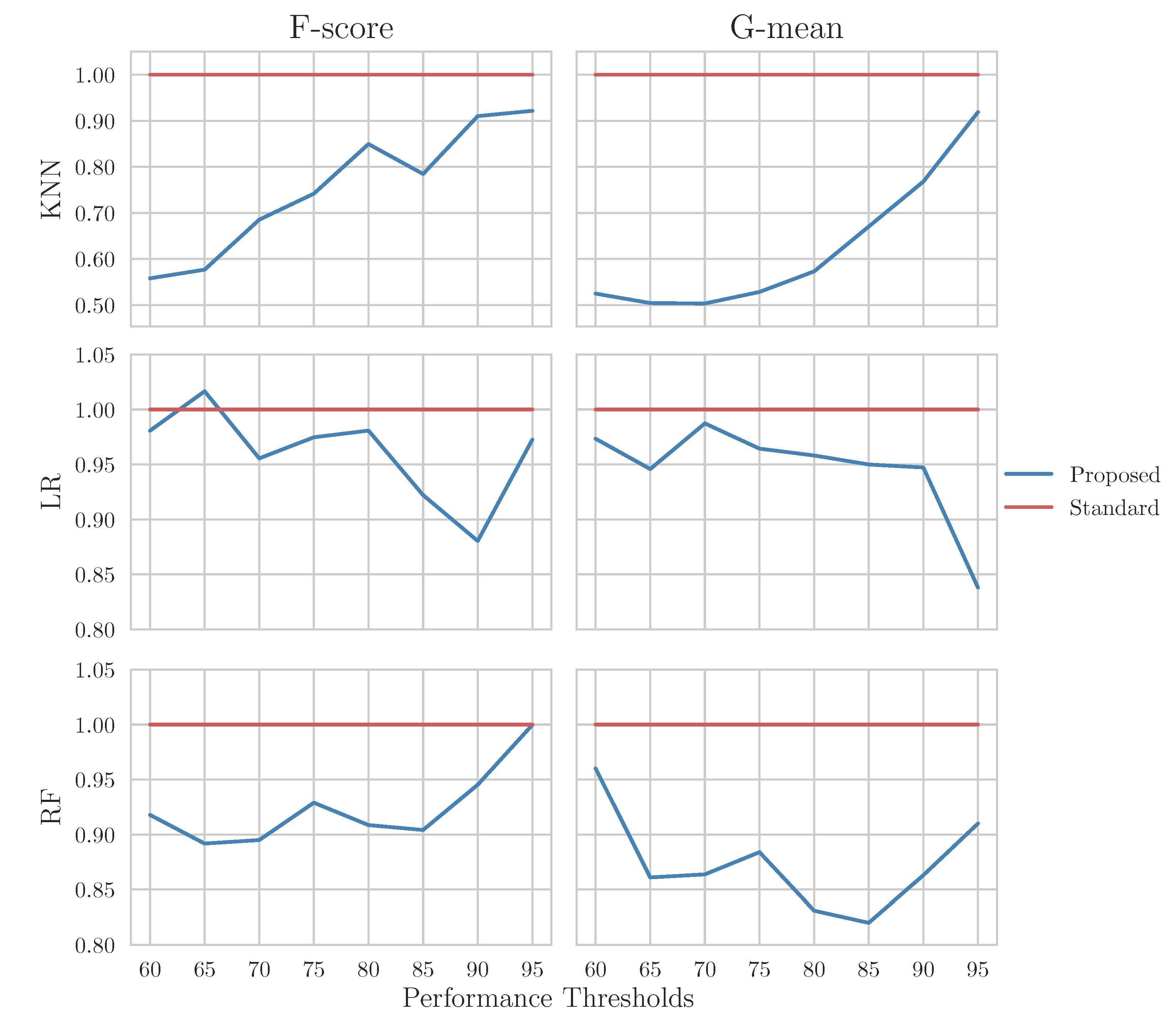
The DUR of the proposed method relative to the baseline method is shown in
Figure 6. A DUR below 1 means that the proposed framework requires fewer data to reach the same performance threshold (as a percentage, relative to the amount of data required by the baseline framework). For instance, in the upper left graphic, we can see that the proposed framework achieves 90% classification using F-score while using 91% of the amount of data used by the traditional AL framework, in other words 9% fewer data.
The averaged optimal classification scores are shown in
Table 7. The maximum performance (MP) classification scores are shown as a benchmark and represent the performance of the corresponding classifier using the entire training set.
6.2. Statistical Analysis
The methods used to test the experiment’s results must be appropriate for a multi-dataset context. Therefore, the statistical analysis is performed using the Wilcoxon signed-rank test [
68] as a post hoc analysis. The variable used for this test is the data utilization rate based on the G-mean performance metric, considering the various performance thresholds in
Table 6.
The Wilcoxon signed-rank test results are shown in
Table 8. We test as null hypothesis that the performance of the proposed framework is the same as the original AL framework. The null hypothesis is rejected in all datasets.
6.3. Discussion
This paper expands the AL framework by adding an artificial data generator into its iterative process. This modification is done to accelerate the classification convergence of the standard AL procedure, which is reflected in the reduction of the amount of data necessary to reach better classification results.
The convergence efficiency of the proposed method is always higher than the baseline AL framework, with the exception of one comparison, as shown in
Table 4 and
Figure 6. This means the proposed AL framework using data generation was able to outperform the baseline AL in nearly all scenarios.
The mean AULC scores in
Table 5 show a significant improvement in the performance of AL when a generator is used. The mean performance of the proposed framework is always better than the baseline framework. This improvement is explained by:
There is earlier convergence of AL, i.e., it requires fewer data to achieve comparable performance levels. This effect is shown in
Table 6, where we found that the proposed framework always uses fewer data for similar performance levels, regardless of the classifier used.
There is higher optimal classification performance, i.e., it reaches higher performance levels overall. This effect is shown in
Table 7, where we found that using a generator in AL led to a better classification performance and the capability of outperforming the MP threshold.
Our results show statistical significance in every dataset. The proposed framework had a superior performance with statistical significance on each dataset at a level of . This indicates that, regardless of the context under which an AL algorithm is used, the proposed framework reduces the amount of data necessary in the AL’s iterative process.
This paper introduces the concept of applying a data generation algorithm in the AL framework. This was done with the implementation of a recent state-of-the-art generalization of a popular data generation algorithm. However, since this algorithm is based on heuristics, future work should focus on improving these results through the design of new data generation mechanisms, at the cost of additional computational power. In addition, we also noticed significant standard errors in our experimental results (see
Section 6.1). This indicates that AL procedures seem to be particularly sensitive to the initialization method, which is still a limitation of AL, regardless of the framework and configurations used. This is consistent with the findings in [
22], which future work should attempt to address. Although using a generator marginally reduced this standard error, it is not sufficient to address this specific limitation.
7. Conclusions
The aim of this experiment was to test the effectiveness of a new AL framework that introduces artificial data generation in its iterative process. The experiment was designed to test the proposed method under particularly challenging conditions, where the maximum performance line is naturally high in most datasets. The element that constitutes the generator component was set up in a plug-and-play scheme, without significant tuning of the G-SMOTE oversampler. Using a generator in AL improved the original AL framework in all scenarios. These results could be further improved through the modification and more intense tuning of the data generation strategy. In our experiment, artificial data were generated only to match each non-majority class frequency with the majority class frequency, strictly balancing the class distribution. Generating a larger amount of data for all classes can further improve these results.
The high performance scores for the baseline AL framework made the achievement of significant improvements over the traditional AL framework under these conditions particularly meaningful. The advantage of the proposed AL framework is shown in
Table 6. In most of the presented scenarios, there is a substantial reduction of data necessary to reach a given performance threshold.
The results from this experiment show that using a data generator in the AL framework will improve the convergence of the method. This framework successfully anticipates the predictor’s optimal performance, as shown in
Table 4,
Table 5 and
Table 6. Therefore, in a real application, the annotation cost would have been reduced since fewer iterations and labeled instances are necessary to reach near optimal classification performance.


