
Matchup Characteristics of Sea Surface Salinity Using a High-Resolution Ocean Model

 , ,
, ,
Abstract
:1. Introduction
2. Data and Methods
2.1. Observations
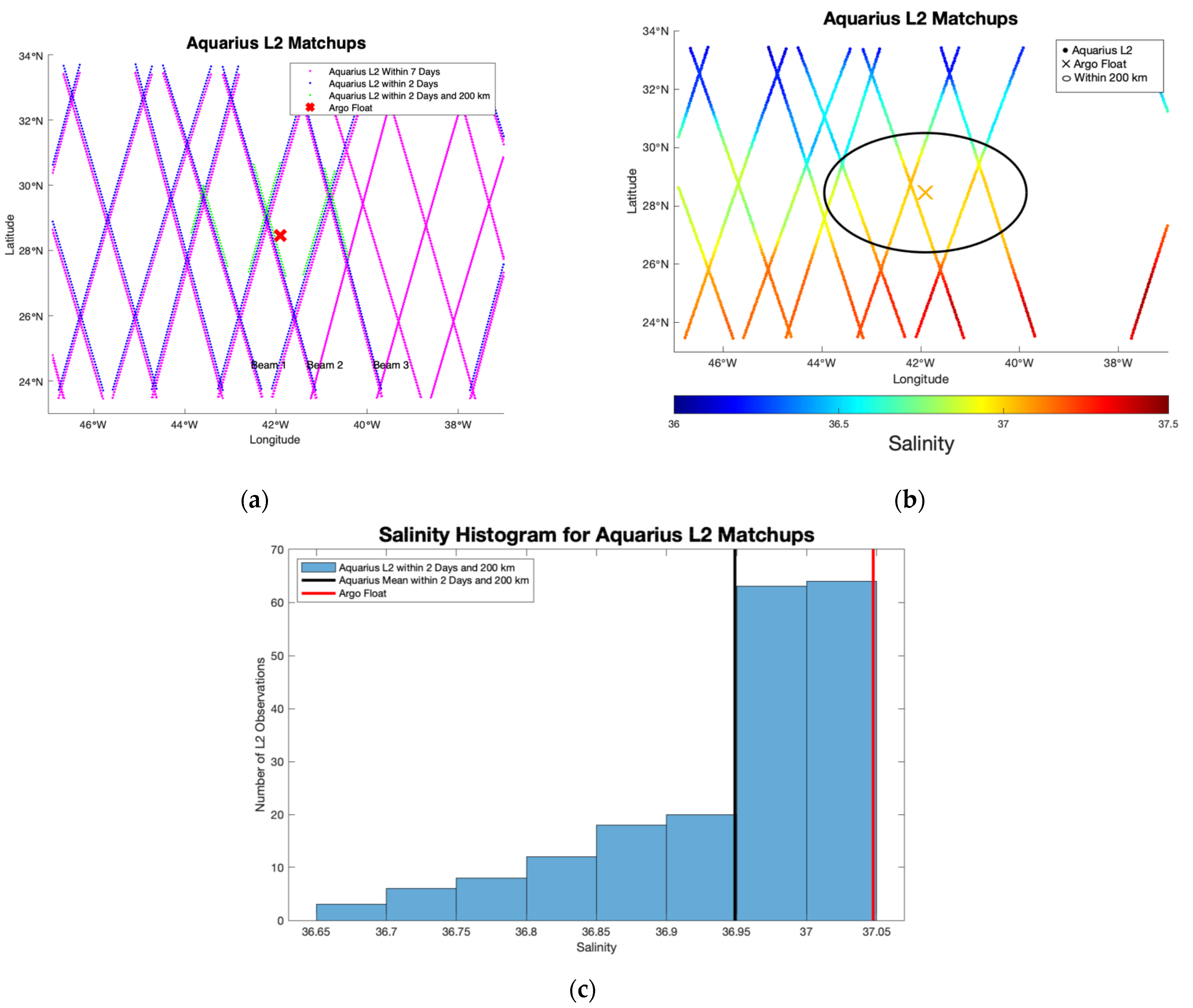
2.1.1. L2 Aquarius
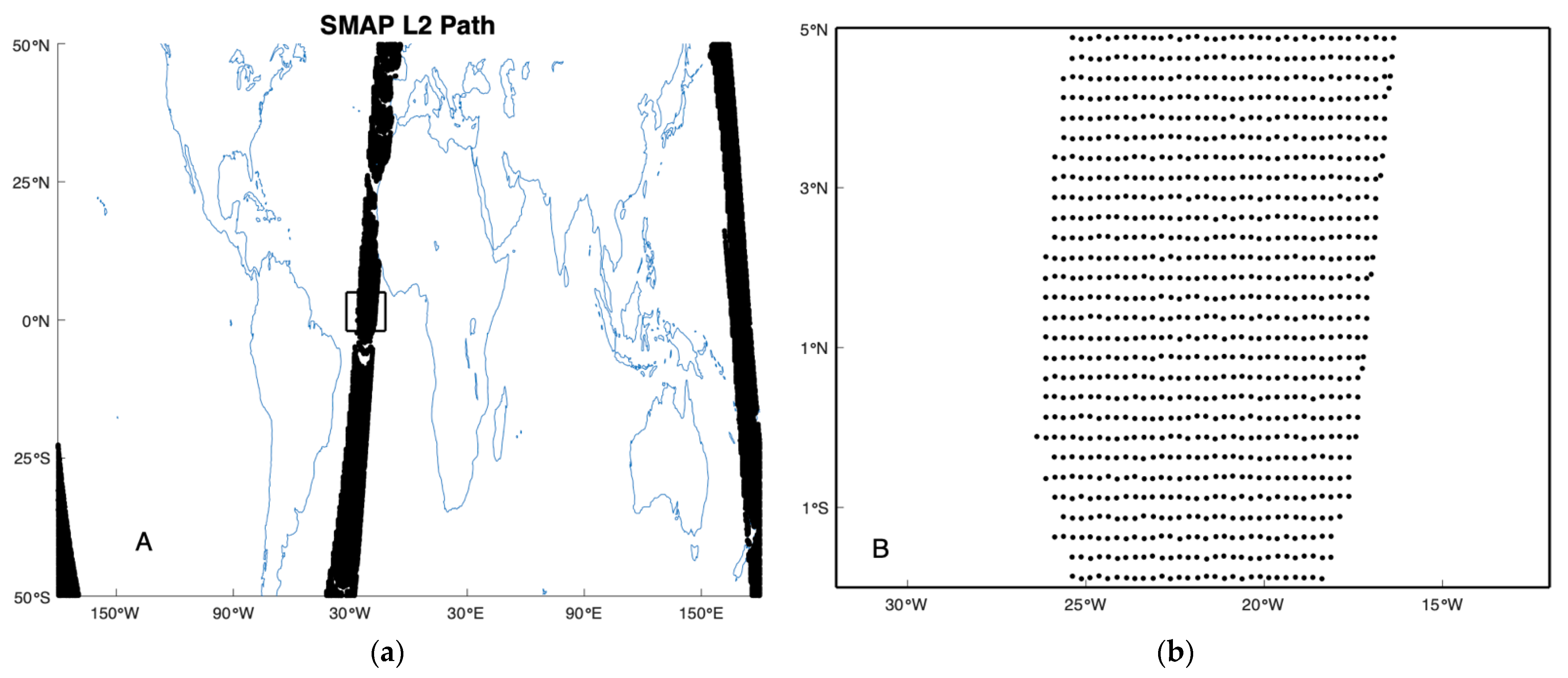
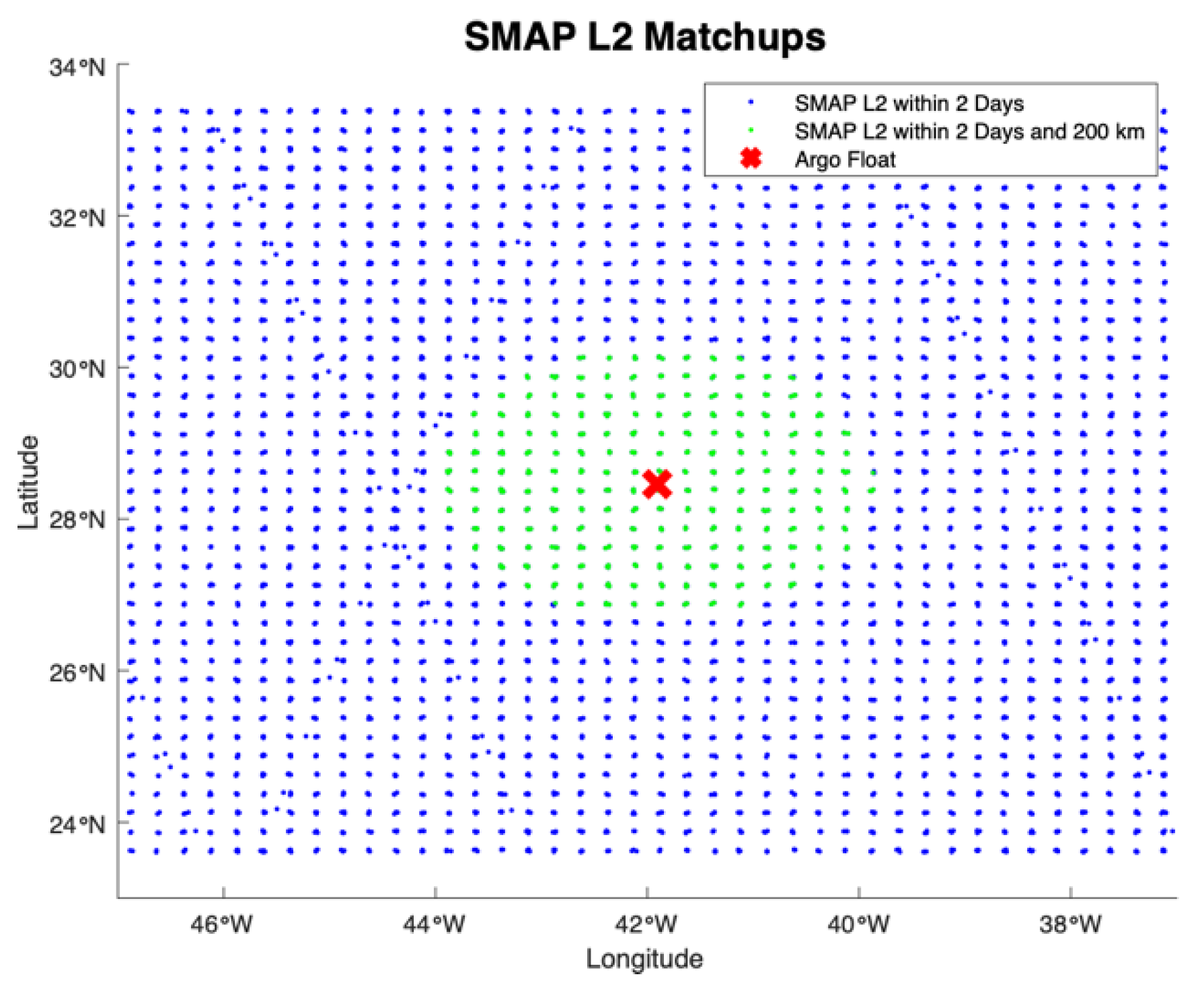
2.1.2. L2 SMAP
2.1.3. Argo
2.2. The MITgcm
2.3. Simulation Data
2.3.1. Simulated Satellite L2
2.3.2. Simulated Argo
2.4. Matchups
3. Results
4. Discussion
Author Contributions
Funding
Data Availability Statement
Acknowledgments
Conflicts of Interest
References
- Vinogradova, N.; Lee, T.; Boutin, J.; Drushka, K.; Fournier, S.; Sabia, R.; Stammer, D.; Bayler, E.; Reul, N.; Gordon, A.; et al. Satellite Salinity Observing System: Recent Discoveries and the Way Forward. Front. Mar. Sci. 2019, 6, 243. [Google Scholar] [CrossRef]
- Meissner, T.; Wentz, F.; Le Vine, D. The salinity retrieval algorithms for the NASA Aquarius version 5 and SMAP version 3 releases. Remote Sens. 2018, 10, 1121. [Google Scholar] [CrossRef] [Green Version]
- Olmedo, E.; González-Haro, C.; Hoareau, N.; Umbert, M.; González-Gambau, V.; Martínez, J.; Gabarró, C.; Turiel, A. Nine years of SMOS sea surface salinity global maps at the Barcelona Expert Center. Earth Syst. Sci. Data 2021, 13, 857–888. [Google Scholar] [CrossRef]
- Reul, N.; Grodsky, S.A.; Arias, M.; Boutin, J.; Catany, R.; Chapron, B.; D’Amico, F.; Dinnat, E.; Donlon, C.; Fore, A.; et al. Sea surface salinity estimates from spaceborne L-band radiometers: An overview of the first decade of observation (2010–2019). Remote Sens. Environ. 2020, 242, 111769. [Google Scholar] [CrossRef]
- Roemmich, D.; Gilson, J. The 2004–2008 mean and annual cycle of temperature, salinity, and steric height in the global ocean from the Argo Program. Prog. Oceanogr. 2009, 82, 81. [Google Scholar] [CrossRef]
- Good, S.A.; Martin, M.J.; Rayner, N.A. EN4: Quality controlled ocean temperature and salinity profiles and monthly objective analyses with uncertainty estimates. J. Geophys. Res. Ocean. 2013, 118, 6704–6716. [Google Scholar] [CrossRef]
- Bao, S.; Wang, H.; Zhang, R.; Yan, H.; Chen, J. Comparison of Satellite-Derived Sea Surface Salinity Products from SMOS, Aquarius, and SMAP. J. Geophys. Res. Ocean. 2019, 124, 1932–1944. [Google Scholar] [CrossRef]
- Kao, H.-Y.; Lagerloef, G.S.; Lee, T.; Melnichenko, O.; Meissner, T.; Hacker, P. Assessment of Aquarius Sea Surface Salinity. Remote Sens. 2018, 10, 1341. [Google Scholar] [CrossRef] [Green Version]
- Kao, H.-Y.; Lagerloef, G.; Lee, T.; Melnichenko, O.; Hacker, P. Aquarius Salinity Validation Analysis; Data Version 5.0; Aquarius/SAC-D: Seattle, WA, USA, 2018; p. 45. [Google Scholar]
- Tang, W.; Fore, A.; Yueh, S.; Lee, T.; Hayashi, A.; Sanchez-Franks, A.; Martinez, J.; King, B.; Baranowski, D. Validating SMAP SSS with in situ measurements. Remote Sens. Environ. 2017, 200, 326–340. [Google Scholar] [CrossRef] [Green Version]
- Fournier, S.; Lee, T. Seasonal and Interannual Variability of Sea Surface Salinity Near Major River Mouths of the World Ocean Inferred from Gridded Satellite and In-Situ Salinity Products. Remote Sens. 2021, 13, 728. [Google Scholar] [CrossRef]
- Lee, T. Consistency of Aquarius sea surface salinity with Argo products on various spatial and temporal scales. Geophys. Res. Lett. 2016, 43, 3857–3864. [Google Scholar] [CrossRef] [Green Version]
- Abe, H.; Ebuchi, N. Evaluation of sea-surface salinity observed by Aquarius. J. Geophys. Res. Ocean. 2014, 119, 8109–8121. [Google Scholar] [CrossRef]
- Vazquez-Cuervo, J.; Gomez-Valdes, J.; Bouali, M.; Miranda, L.E.; Van der Stocken, T.; Tang, W.; Gentemann, C. Using Saildrones to Validate Satellite-Derived Sea Surface Salinity and Sea Surface Temperature along the California/Baja Coast. Remote Sens. 2019, 11, 1964. [Google Scholar] [CrossRef] [Green Version]
- Olmedo, E.; Gabarró, C.; González-Gambau, V.; Martínez, J.; Ballabrera-Poy, J.; Turiel, A.; Portabella, M.; Fournier, S.; Lee, T. Seven Years of SMOS Sea Surface Salinity at High Latitudes: Variability in Arctic and Sub-Arctic Regions. Remote Sens. 2018, 10, 1772. [Google Scholar] [CrossRef] [Green Version]
- Olmedo, E.; Martínez, J.; Turiel, A.; Ballabrera-Poy, J.; Portabella, M. Debiased non-Bayesian retrieval: A novel approach to SMOS Sea Surface Salinity. Remote Sens. Environ. 2017, 193, 103–126. [Google Scholar] [CrossRef]
- Bingham, F.M.; Brodnitz, S.; Yu, L. Sea Surface Salinity Seasonal Variability in the Tropics from Satellites, Gridded In Situ Products and Mooring Observations. Remote Sens. 2021, 13, 110. [Google Scholar] [CrossRef]
- Dinnat, E.P.; Le Vine, D.M.; Boutin, J.; Meissner, T.; Lagerloef, G. Remote Sensing of Sea Surface Salinity: Comparison of Satellite and in situ Observations and Impact of Retrieval Parameters. Remote Sens. 2019, 11, 750. [Google Scholar] [CrossRef] [Green Version]
- Qin, S.; Wang, H.; Zhu, J.; Wan, L.; Zhang, Y.; Wang, H. Validation and correction of sea surface salinity retrieval from SMAP. Acta Oceanol. Sin. 2020, 39, 148–158. [Google Scholar] [CrossRef]
- Fournier, S.; Lee, T.; Tang, W.; Steele, M.; Olmedo, E. Evaluation and Intercomparison of SMOS, Aquarius, and SMAP Sea Surface Salinity Products in the Arctic Ocean. Remote Sens. 2019, 11, 3043. [Google Scholar] [CrossRef] [Green Version]
- Vinogradova, N.T.; Ponte, R.M. Small-scale variability in sea surface salinity and implications for satellite-derived measurements. J. Atmos. Ocean. Technol. 2013, 30, 2689–2694. [Google Scholar] [CrossRef]
- Boutin, J.; Chao, Y.; Asher, W.E.; Delcroix, T.; Drucker, R.; Drushka, K.; Kolodziejczyk, N.; Lee, T.; Reul, N.; Reverdin, G. Satellite and in situ salinity: Understanding near-surface stratification and subfootprint variability. Bull. Am. Meteorol. Soc. 2016, 97, 1391–1407. [Google Scholar] [CrossRef] [Green Version]
- Drushka, K.; Asher, W.E.; Sprintall, J.; Gille, S.T.; Hoang, C. Global patterns of submesoscale surface salinity variability. J. Phys. Oceanogr. 2019, 49, 1669–1685. [Google Scholar] [CrossRef]
- Bingham, F.M. Subfootprint Variability of Sea Surface Salinity Observed during the SPURS-1 and SPURS-2 Field Campaigns. Remote Sens. 2019, 11, 2689. [Google Scholar] [CrossRef] [Green Version]
- Schanze, J.J.; Le Vine, D.M.; Dinnat, E.P.; Kao, H.-Y. Comparing Satellite Salinity Retrievals with In Situ Measurements: A Recommendation for Aquarius and SMAP (Version 1); Earth & Space Research: Seattle, WA, USA, 2020; p. 20. [Google Scholar] [CrossRef]
- Su, Z.; Wang, J.; Klein, P.; Thompson, A.F.; Menemenlis, D. Ocean submesoscales as a key component of the global heat budget. Nat. Commun. 2018, 9, 775. [Google Scholar] [CrossRef] [PubMed] [Green Version]
- Donlon, C. Copernicus Imaging Microwave Radiometer (CIMR) Mission Requirements Document; Earth and Mission Science Division, European Space Agency: Noordwijk, The Netherlands, 2020; p. 217. [Google Scholar]
- Physical Oceanography Distributed Active Archive Center (PODAAC). AQUARIUS USER GUIDE Aquarius Dataset Version 5.0; Jet Propulsion Laboratory, California Institute of Technology: Pasadena, CA, USA, 2017; p. 98.
- NASA Aquarius Project. Aquarius Official Release Level 2 Sea Surface Salinity & Wind Speed Data V5.0; Jet Propulsion Laboratory, California Institute of Technology: Pasadena, CA, USA, 2017. [CrossRef]
- Lagerloef, G.S.; Colomb, F.R.; Le Vine, D.M.; Wentz, F.; Yueh, S.; Ruf, C.; Lilly, J.; Gunn, J.; Chao, Y.; deCharon, A.; et al. The Aquarius/SAC-D Mission: Designed to Meet the Salinity Remote-sensing Challenge. Oceanography 2008, 20, 68–81. [Google Scholar] [CrossRef] [Green Version]
- Bingham, F.M.; Howden, S.D.; Koblinsky, C.J. Sea surface salinity measurements in the historical database. J. Geophys. Res. C Ocean. 2002, 107, 8019. [Google Scholar] [CrossRef]
- Remote Sensing Systems (RSS). RSS SMAP Level 2C Sea Surface Salinity V4.0 Validated Dataset; RSS: Santa Rosa, CA, USA, 2019. [Google Scholar] [CrossRef]
- Dai, A.; Trenberth, K.E. Estimates of Freshwater Discharge from Continents: Latitudinal and Seasonal Variations. J. Hydrometeorol. 2002, 3, 660. [Google Scholar] [CrossRef] [Green Version]
- Menemenlis, D.; Campin, J.-M.; Heimbach, P.; Hill, C.; Lee, T.; Nguyen, A.; Schodlok, M.; Zhang, H. ECCO2: High Resolution Global Ocean and Sea Ice Data Synthesis. Mercator Ocean Q. Newsl. 2008, 31, 13–21. [Google Scholar]
- Bingham, F.M.; Lee, T. Space and time scales of sea surface salinity and freshwater forcing variability in the global ocean (60° S–60° N). J. Geophys. Res. Ocean. 2017, 122, 2909–2922. [Google Scholar] [CrossRef]
- Meissner, T.; Wentz, F.; Manaster, A.; Lindsley, R. NASA/RSS SMAP Salinity: Version 3.0 Validated Release; Remote Sensing Systems: Santa Rosa, CA, USA, 2019. [Google Scholar]
- Kuusela, M.; Stein, M.L. Locally stationary spatio-temporal interpolation of Argo profiling float data. Proc. R. Soc. A 2018, 474. [Google Scholar] [CrossRef] [Green Version]
- Bingham, F.M.; Li, Z. Spatial Scales of Sea Surface Salinity Subfootprint Variability in the SPURS Regions. Remote Sens. 2020, 12, 3996. [Google Scholar] [CrossRef]
- Drucker, R.; Riser, S.C. Validation of Aquarius sea surface salinity with Argo: Analysis of error due to depth of measurement and vertical salinity stratification. J. Geophys. Res. Ocean. 2014, 119, 4626–4637. [Google Scholar] [CrossRef]
- Boyer, T.P.; Levitus, S. Harmonic Analysis of Climatological Sea Surface Salinity. J. Geophys. Res. 2002, 107, 8006. [Google Scholar] [CrossRef]
- Yu, L.; Bingham, F.M.; Lee, T.; Dinnat, E.P.; Fournier, S.; Melnichenko, O.; Tang, W.; Yueh, S.H. Revisiting the Global Patterns of Seasonal Cycle in Sea Surface Salinity. J. Geophys. Res. Ocean. 2021, 126, e2020JC016789. [Google Scholar] [CrossRef]


| Reference | Comparison |
|---|---|
| [13] | L2 compared to Argo within 12 h and 200 km. |
| [8,9] | Searched for the closest point of approach (CPA) of the satellite to each Argo float. Time window ±3.5 days and space window 75 km; 11 L2 samples averaged for comparison with the float value. |
Publisher’s Note: MDPI stays neutral with regard to jurisdictional claims in published maps and institutional affiliations. |
© 2021 by the authors. Licensee MDPI, Basel, Switzerland. This article is an open access article distributed under the terms and conditions of the Creative Commons Attribution (CC BY) license (https://creativecommons.org/licenses/by/4.0/).
Share and Cite
Bingham, F.M.; Fournier, S.; Brodnitz, S.; Ulfsax, K.; Zhang, H. Matchup Characteristics of Sea Surface Salinity Using a High-Resolution Ocean Model. Remote Sens. 2021, 13, 2995. https://doi.org/10.3390/rs13152995
Bingham FM, Fournier S, Brodnitz S, Ulfsax K, Zhang H. Matchup Characteristics of Sea Surface Salinity Using a High-Resolution Ocean Model. Remote Sensing. 2021; 13(15):2995. https://doi.org/10.3390/rs13152995
Chicago/Turabian StyleBingham, Frederick M., Severine Fournier, Susannah Brodnitz, Karly Ulfsax, and Hong Zhang. 2021. "Matchup Characteristics of Sea Surface Salinity Using a High-Resolution Ocean Model" Remote Sensing 13, no. 15: 2995. https://doi.org/10.3390/rs13152995
APA StyleBingham, F. M., Fournier, S., Brodnitz, S., Ulfsax, K., & Zhang, H. (2021). Matchup Characteristics of Sea Surface Salinity Using a High-Resolution Ocean Model. Remote Sensing, 13(15), 2995. https://doi.org/10.3390/rs13152995