Abstract
Local and Regional Authorities require indicators at the intra-urban scale to design adequate policies to foster the achievement of the objectives of Sustainable Development Goal (SDG) 11. Updated high-resolution population density and settlement maps are the basic input products for such indicators and their sub-indicators. When provided at the intra-urban scale, these essential variables can facilitate the extraction of population flows, including both local and regular migrant components. This paper discusses a modification of the dasymetric method implemented in our previous work, aimed at improving the population density estimation. The novelties of our paper include the introduction of building height information and site-specific weight values for population density correction. Based on the proposed improvements, selected indicators/sub-indicators of four SDG 11 targets were updated or newly implemented. The output density map error values are provided in terms of the mean absolute error, root mean square error and mean absolute percentage indicators. The values obtained (i.e., 2.3 and 4.1 people, and 8.6%, respectively) were lower than those of the previous dasymetric method. The findings suggest that the new methodology can provide updated information about population fluxes and processes occurring over the period 2011–2020 in the study site—Bari city in southern Italy.
1. Introduction
Updated high-resolution population density maps of urban settlements have been recognized as essential variables for the calculating of Sustainable Development Goal (SDG) 11 indicators (i.e., Make cities and human settlements inclusive, safe, resilient, and sustainable) [1] in the framework of the United Nations 2030 Agenda [2]. In order to monitor the achievements of such goals, Local and Regional Authorities (LRAs) play a key role in pursuing SDGs [3]. In this regard, the New Urban Agenda (NUA) adopted by [4], suggests actively involving LRAs in a bottom-up strategy of SDG 11 process acceleration; however, LRAs require products at a fine intra-urban scale, whereas the current literature provides only national or global scale indicators [5,6,7,8,9].
In our previous work [10], a vector-based dasymetric method was implemented to generate a population density and distribution map on a grid (100 m × 100 m), by combining census data with an updated settlement map obtained from Sentinel-2 data. The study area was the municipality of Bari, southern Italy, interested in migration fluxes monitoring.
In this study, a new version of the vector-based dasymetric method is proposed to provide both updated and more reliable population density maps at the intra-urban scale for the same urban area. The area has been exposed to increasing migration processes and fluxes of the local and migrant population, which deserve attention, considering cohesion and inclusion issues. Thus, a map was produced for both the total urban population and its regular migrant component, for each continent of origin.
The main innovation of the presented work is related to the introduction of building height information in the dasymetric formula. According to recent research efforts, the use of building height for building volume estimation production seems to provide more reliable output population density maps, thus reducing population density uncertainties. At the global scale, [11] suggested the use of a Digital Elevation Model (DEM). They found a composite of the 1-arcsec Shuttle Radar Topography Mission (SRTM30) and the Advanced Land Observing Satellite (ALOS) World 3D–30 m to be a reliable DEM source for estimating the vertical component of built-up areas. At the national scale, [12] combined Sentinel-1A/B and Sentinel-2A/B time-series to map building heights using a machine learning regression model. The authors found that good performance can be achieved with frequency-weighted RMSE values ranging from 2.9 m to 3.5 m. However, the model used in their study had to be trained and validated with highly accurate building height data from several 3D building models to obtain reliable values. At the local scale, [13] suggested estimating building height and building footprint area from Synthetic Aperture Radar (SAR)PALSAR-2 (onboard ALOS-2), which has a very high spatial resolution. They found that the use of SAR data can: (1) Enable automated delineation of built-up areas at a spatial resolution of 5 m, with an accuracy of 85% when using globally available low-resolution training data; (2) assess the density of building height class with a root mean square error of 0.25, 0.034 and 0.032 for the low, mid and high-rise building density classes, respectively; (3) deal with the scattering components of buildings at different orientation angles by combining data from both ascending and descending orbits; however, the authors did not apply the proposed technique to demographic studies.
At the intra-urban scale, in [14], the results of different dasymetric methods were compared to introduce volume information into population density evaluation. From LiDAR data, the authors first extracted building footprint areas through threshold values of building heights. Then, they estimated the building volume as a product between 25 square meters cells (including buildings) and their height values. Additionally, the authors used the Urban Atlas (UA) [15], which provides pan-European comparable land cover and land use data for functional urban areas (FUA) to extract building uses. Such information served as an additional input when running the dasymetric method. The reason for this choice was that the geometric accuracy of the Urban Atlas product is greater than that of CORINE Land Cover (CLC): the minimum mapping unit (MMU) ranges from 0.25 to 1 ha in the former product, while it is 25 ha in the latter. From the Urban Atlas, the authors identified buildings with residential use and applied the dasymetric method to such buildings. By using LiDAR data for volume estimation and the Copernicus Urban Atlas the authors obtained better performance, in terms of both mean absolute percentage error (MAPE) and root mean square error (RMSE), with respect to two-dimensional dasymetric methods [14]. Furthermore, the study found that only high-resolution vector information, such as cadastral information, can provide the final best performance; however, cadastral data may either not be regularly updated, such as in Italy or Southern Europe, or is costly.
In this study, to improve the previously implemented dasymetric method [10], according to the findings and suggestions from the mentioned studies, we introduce the following novelties in the dasymetric method at the intra-urban scale: (a) Building height information from LiDAR data, (b) building use information from Copernicus UA layers dated 2012 and 2018, and (c) site-specific weight values for population density correction; such values, instead of the fixed ones used in [10,16], are derived by the ratio of the average population density in non-residential areas to the estimated density in predominantly residential areas. According to the recent literature, the proposed method belongs to the class of hybrid Statistical–Dasymetric Models [17]. While traditional dasymetric models can produce fine-resolution population density estimates through relationships between population distribution and ancillary geographic layers, such as land cover maps [18], an increasing number of hybrid approaches have recently been introduced in the literature [17]. These methods explicitly combine the traditional concept of dasymetric mapping with statistical analytical tools to determine the population allocation weights. The regression of either population counts or densities against various types of predictive variables (e.g., those derived from ancillary layers) was mentioned in the review work of [17]. Such hybrid Statistical–Dasymetric models could ensure both the standardization of the dasymetric procedure and its reproducibility in other study areas.
Based on the proposed improvements, all of the indicators implemented in [10] were updated. These include (a) SDG 11.1.1—“Proportion of urban population living in slums, informal settlements, or inadequate housing” and its sub-indicators (1) and (2), considering inadequate housing for both their structural features and hazardous location; and (b) SDG 11.3.1—“Ratio of land consumption rate to population growth rate”. The following additional indicators/sub-indicators were implemented: SDG 11.1.1 sub-indicator (3) related to building crowding; SDG 11.2.1—“Proportion of population that has convenient access to public transport” in the migrant and total populations; SDG 11.6.2—”Annual mean levels of fine particulate matter (e.g., PM2.5 and PM10) in cities (population-weighted)”.
In the Bari study area, all the indicators listed above as well as their changes (2011–2020) were quantified for both the total population and the regular migrant population components, with distinctions drawn between nationalities of origin.
To the best of our knowledge, in the current literature, not many studies have implemented SDG 11 indicators to provide high-resolution maps that describe the spatial variation of the processes analysed at an intra-urban scale. The studies [19,20] have provided methodologies to estimate SDG 11.1.1 indicators from Earth Observation data at a local level, underlining how uncertainties still affect reporting on SDG indicator 11.1.1, as well as other SDG indicators, such as 11.3.1, which require robust information on population estimates.
2. Materials and Methods
2.1. Study Area
The study area (Figure 1) covers about 260 km2, including the city of Bari in the Apulia region, southern Italy. Other nearby municipalities were not included due to the lack of both open data and common formats useful for our purpose.
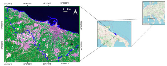
Figure 1.
Study area in the green frame. Bari municipality boundaries are indicated in blue. Background source: Sentinel-2 image, 10 m spatial resolution, acquired on 27 October 2018.
Over the last 20 years, the city of Bari has experienced an upward trend in its migrant population, in contrast to the downward trend in the native population. In the last decade, the overall migratory balance—evaluated with respect to the entire metropolitan area population—has been continuously negative. The local population (especially young people) tend to move towards Northern Italy or abroad for work and study [21,22]. The total population of Bari city remained quite stable up to 2020 (see Table 1) with only an additional total increase of 2.18%, whereas the migrant population increased by about 100% since 2011 (the date of the last ISTAT national survey of the population).

Table 1.
Population data of Bari. Source: ISTAT.
2.2. Satellite-Derived Products
For the present study, we first updated the settlement map of the area under study up to 2020 by using Sentinel-2 imagery. The data selected were multi-seasonal and cloud-free Sentinel-2 images, freely downloaded from the United States Geological Survey (USGS) EarthExplorer portal [23] as Level-2A surface reflectance products. The selected dataset consisted of four images acquired on 25 January, 22 May, 28 July and 4 October 2020. For each image, the four spectral bands at 10 m spatial resolution (i.e., B2, B3, B4 and B8) and the six bands at 20 m (i.e., B5, B6, B7, B8a, B11 and B12) were analysed. The latter six bands were resampled to 10 m spatial resolution using a bilinear function, while the Sentinel-2 spectral bands at 60 m spatial resolution were not used.
The map was obtained from the same pixel-based, data-driven, automatic classification procedure that performed best in our previous work [10]. This approach was possible given the availability of in-situ reference data for training a support vector machine (SVM) classifier [24]. The 10 image spectral bands were used as input to the classifier along with slope measurements obtained from the available digital elevation model (DEM). The DEM, at 8 m spatial resolution, was added as input for discriminating built-up objects from extraction sites. For the SVM classifier, a radial basis function (RBF) was adopted as the kernel function and the training parameters were as follows: gamma = 0.024 and regularization parameter (C) = 100. The Food and Agriculture Organization Land Cover Classification System (FAO–LCCS) taxonomy was considered for class discrimination [25]. The classifier was trained for a multi-class problem considering the following Land Cover (LC) classes: B15/A1 (Artificial Structures/Built-Up); B15/A2A6 (Artificial Structures/Extraction sites); (B27 or B28)/A1 (Artificial or Natural Water Bodies/Water); A11/(A1 or A2)A9 or A12/(A3 or A4)E1 (Cultivated Lands or Natural Vegetation/(Evergreen Trees or Shrubs); A11/(A1 or A2)A10 or A12/(A3 or A4)E2 (Cultivated Lands or Natural Vegetation/(Deciduous Trees or Shrubs); A12/A2 (Natural Vegetation/Herbaceous); A11/A3 (Cultivated Lands/Herbaceous). The output LC map was produced by training the SVM classifier with 11,892 references unchanged pixels. The final 2020 binary settlement map, with buildings only and at 10 m spatial resolution, was validated using a set of 3403 reference pixels. Both training and validation reference pixels were selected according to a stratified random sampling to obtain a sample population in which all the classes were neither over- nor under-represented [26].
2.3. Statistical Census Data
Population data per census area were used as the main input for generating the population density map on a fine grid. At the intra-urban scale, all issues related to such data collection and format harmonization were discussed in [10].
Every year, the Italian National Institute of Statistics (ISTAT) publishes data concerning the total number of residents in each municipality classified by sex, nationality and age. The latest updated data, specified per census zone, relate to the 2011 National Census Collection. As of 2018, the ISTAT Permanent Population Census came into force. However, to date, population data at intra-urban scales have not yet been published by ISTAT; the last update was on 9 October 2011. Thus, at the local level, the acquisition of statistics data per census zone, updated on 1 January 2020, was obtained through interaction and collaboration with the Demographic Service Office of Bari municipality.
The tabular data provided by ISTAT and the Demographic Service Office of Bari were transposed onto maps represented in the Universal Transverse Mercator Coordinate System (European Terrestrial Reference System 1989) and ingested in the open-source QGIS environment (Figure 2).
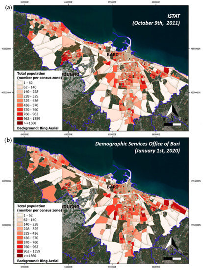
Figure 2.
The total population per census zone of Bari in 2011 (a) and 2020 (b). Background source: Bing Aerial.
2.4. Building Use Information
Dasymetric mapping is used as a tool to disaggregate census data at the landscape level [10,16]. The basic principle of dasymetric mapping is to sub-divide source zones into smaller spatial units possess greater internal consistency of the variable being mapped. Boundaries represented on dasymetric maps reflect spatial distribution data of actual population distribution, rather than the artificially imposed limits (e.g., administrative boundaries) of areal units [10]. The method requires, as input, a built-up map weighting depending on the building use for each area. In our previous paper, weight values were the same as those used in [16].
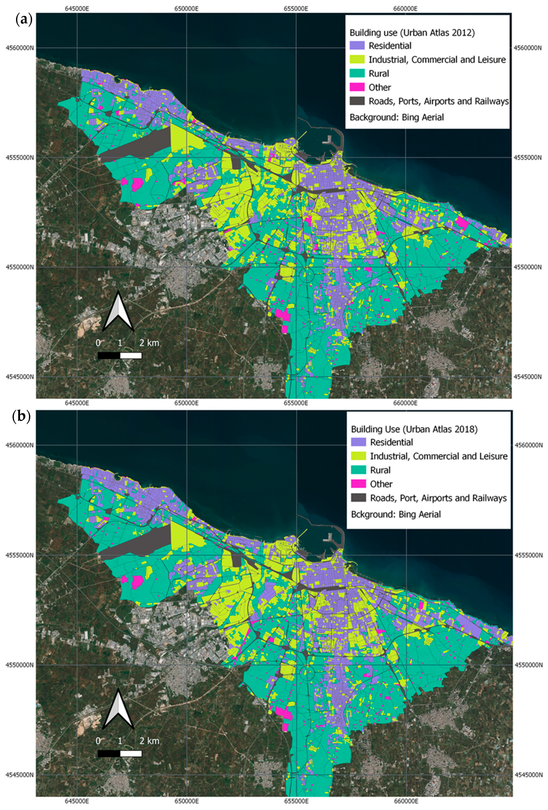
In this study, we propose a new version of the dasymetric method which, instead, extracts building use information from the Copernicus UA service available for 2012 and recently updated to 2018 [15]. The UA classes are aggregated according to the type of building use, based on the associations shown in Table 2. The resultant maps are depicted in Figure 3.

Table 2.
Building use classes.
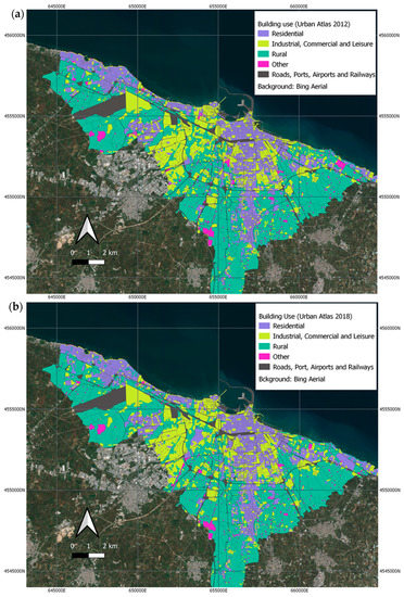
Figure 3.
Building use information extracted from Urban Atlas 2012 (a) and 2018 (b) provided by Copernicus Land Monitoring Services. Background source: Bing Aerial.
2.5. Dasymetric Mapping Method (Version 2.0)
According to [10], population data, at the census level, can be disaggregated and reallocated to each cell of the output grid (100 m × 100 m).
The criteria proposed in the present work to define the weights of population redistribution are described as follows:
- In residential areas, population allocation is proportional to building volumes.
- In non-residential areas, population allocation in a specific cell depends on building use as well as volumes.
Such criteria were supported by the results of the statistical analysis described in Section 3.1.2. Moreover, many authors [16,27,28,29] have endorsed the dependency between population density and land use maps informing on residential, rural and industrial/commercial areas. In particular, [16] introduced a correction factor for the dasymetric weights to be applied to non-residential areas.
To evaluate building volumes, first, building footprint areas were estimated from the updated settlement map obtained from Sentinel-2 data. Then, building height values were extracted from LiDAR data, which had been acquired by the Italian Ministry of the Environment (new Ministry of Ecological Transition), within the “Extraordinary Remote Sensing Plan,” and were based on surveys held in 2008.
The introduction of building height information can discriminate between residential areas of greater or lesser density. This hypothesis was reinforced by the statistical analysis conducted in Section 3.1.2. Based on building heights, built-up in historical areas, characterized by buildings with a maximum of 3 floors, could be differentiated from modern multi-floor buildings, and villas/independent houses with 1–2 floors.
In this study, the assumption was made that, in non-residential areas with predominantly industrial, commercial or other uses, population density is not related to building volume. Therefore, a correction factor for the weights, according to the building use, was determined by comparing the average density of non-residential areas with that of predominantly residential areas. These coefficients were no longer fixed as in [10,16] but were site-specific. The results obtained are reported in Section 3.1.2.
In Table 3, the list of all novelties in the new dasymetric method.

Table 3.
List of novelties introduced with respect to the previous version of the method.
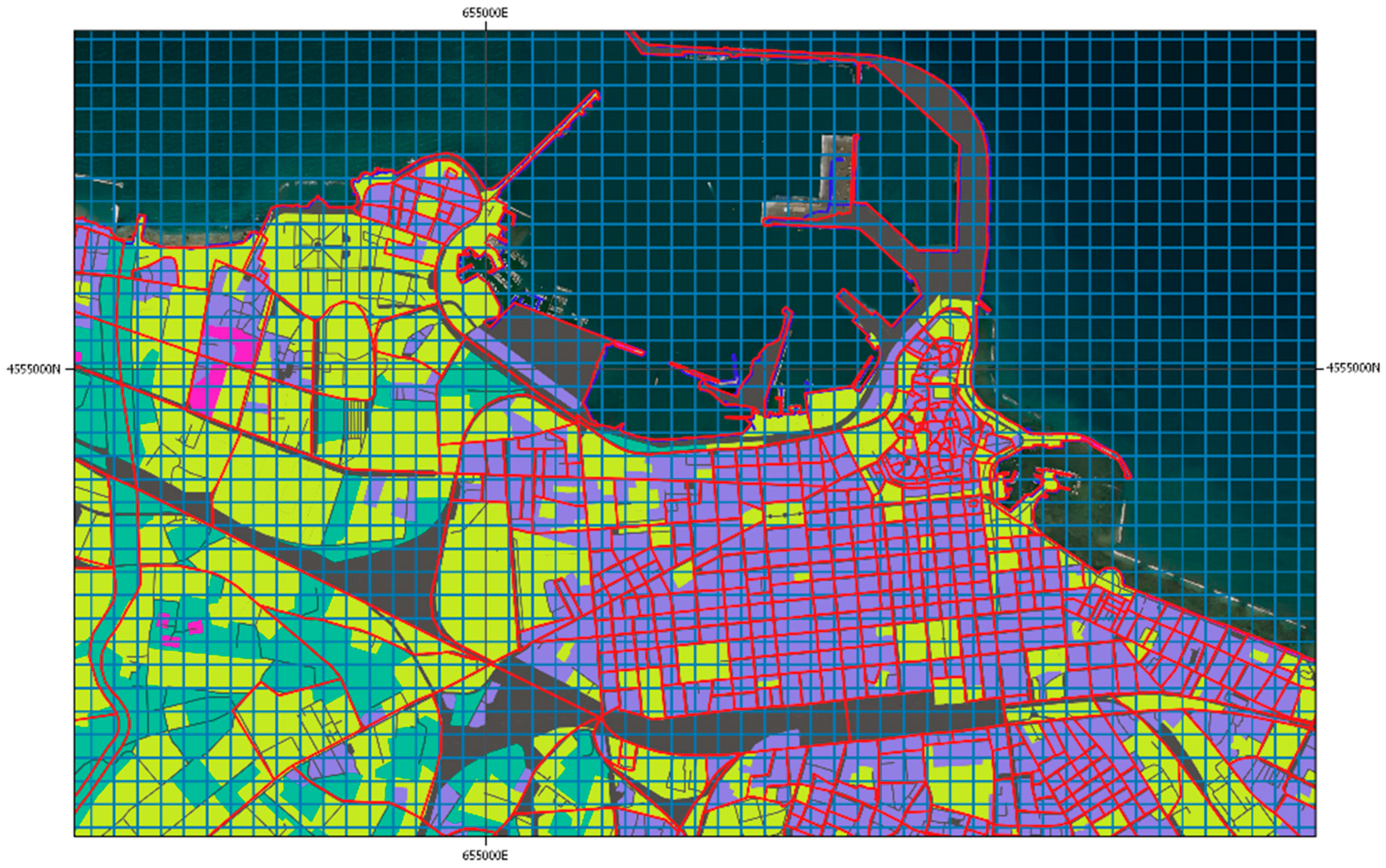
The first step of the dasymetric method consists of a double intersection of the input vector information layers: polygons of census areas; polygons of different building uses and the final output grid. The elements resulting from such double intersections are shown in Figure 4. The colours represent the different building uses. The red strokes identify the polygons of the census areas, while the blue strokes delimit the output grid cells.

Figure 4.
Double intersection of input vector layers.
The following formula reflects the dasymetric computation method implemented in the QGIS environment
where,
- is the built-up footprint area in a generic sub-element of a census zone having different building use;
- is the number of census zone sub-elements with different building use, derived from the intersection of vector layers census zones and building use;
- is the built-up footprint area in a generic sub-element of a census zone, with different building use, included in the output cell considered;
- is the number of census zones sub-elements, with different building uses, within a grid cell, derived from the double intersection;
- is the population of a generic census zone;
- is the number of census zones in a cell;
- is the final population allocated to a cell of a regular grid;
- is a mean value of building heights of sub-elements in a cell;
- is a mean value of building heights in census zones;
- are correction factors based on building uses, as described in Section 3.1.2.
The choice of evaluating heights as an average in the LiDAR set (dated 2008) is a criterion that is useful to overcome the issue of missing information for buildings constructed after 2008. Such an approximation is justified by the existence of municipal regulations [30] that prevent the construction of new buildings with height values differing from those prevailing in the urban context.
The block diagram of the software implementation in the QGIS environment (compatible with versions based on Python 3.7) is shown in Figure 5.
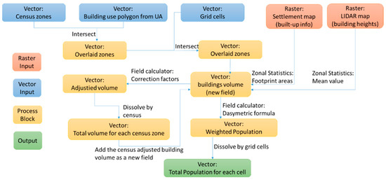
Figure 5.
Dasymetric 2.0 version.
2.6. Quantifiable Derivatives of SDG 11 Indicators and Required Ancillary Data
A complete list of SDG 11 indicators developed for the case study, along with the metrics, derivatives and ancillary data used for measuring them is provided in Table 4. The ancillary data required as input were from local providers. However, the data were not up-to-date or in the same format. This may require time-consuming data pre-processing or have impacts on final accuracy values.

Table 4.
List of ancillary data needed to evaluate SDG 11 indicators at intra-urban scale. bold format is used to identify the new indicators implemented.
The fine-grid population density map was used as an input for all the indicators in Table 4, while the settlement map, which can be updated from satellite data, was used as an input for SDGs 11.1.1 and 11.3.1 only. Except for the indicator SDG 11.3.1, all the others required ancillary data as input.
In Table 4, we denote the newly implemented indicators with bold characters.
2.7. SDG 11.1.1 Indicator
For the implementation of the indicator SDG 11.1.1 “Proportion of urban population living in slums, informal settlements or inadequate housing” several calculation methods were developed depending on the meaning of “inadequate”:
- sub-indicator (1) the “proportion of households with non-durable housing”;
- sub-indicator (2) the “proportion of households living in housing residing on or near hazardous areas”;
- sub-indicator (3) “proportion of households with insufficient living space”.
In the absence of local information layers to be used as ground truth and very high-resolution EO data, in this work, we considered all buildings, without distinguishing the slums from the houses.
To quantify sub-indicators (1) and (2), the procedures remained unchanged from those presented in [10,31]. Unlike the previous work, the analysis concerned the total population, instead of only the regular migrant component. Furthermore, the population grid was used as input to calculate the cumulative number of people potentially living in “inadequate housing”. This value can be used to compare results obtained at the intra-urban spatial disaggregation level with outcomes achieved at an urban scale.
As in [10], the ancillary building use layer, provided by Bari municipality in the “civilario comunale” dataset (2017), provided useful information on the number and position of inadequate housing with structural deficiencies as an input for sub-indicator (1).
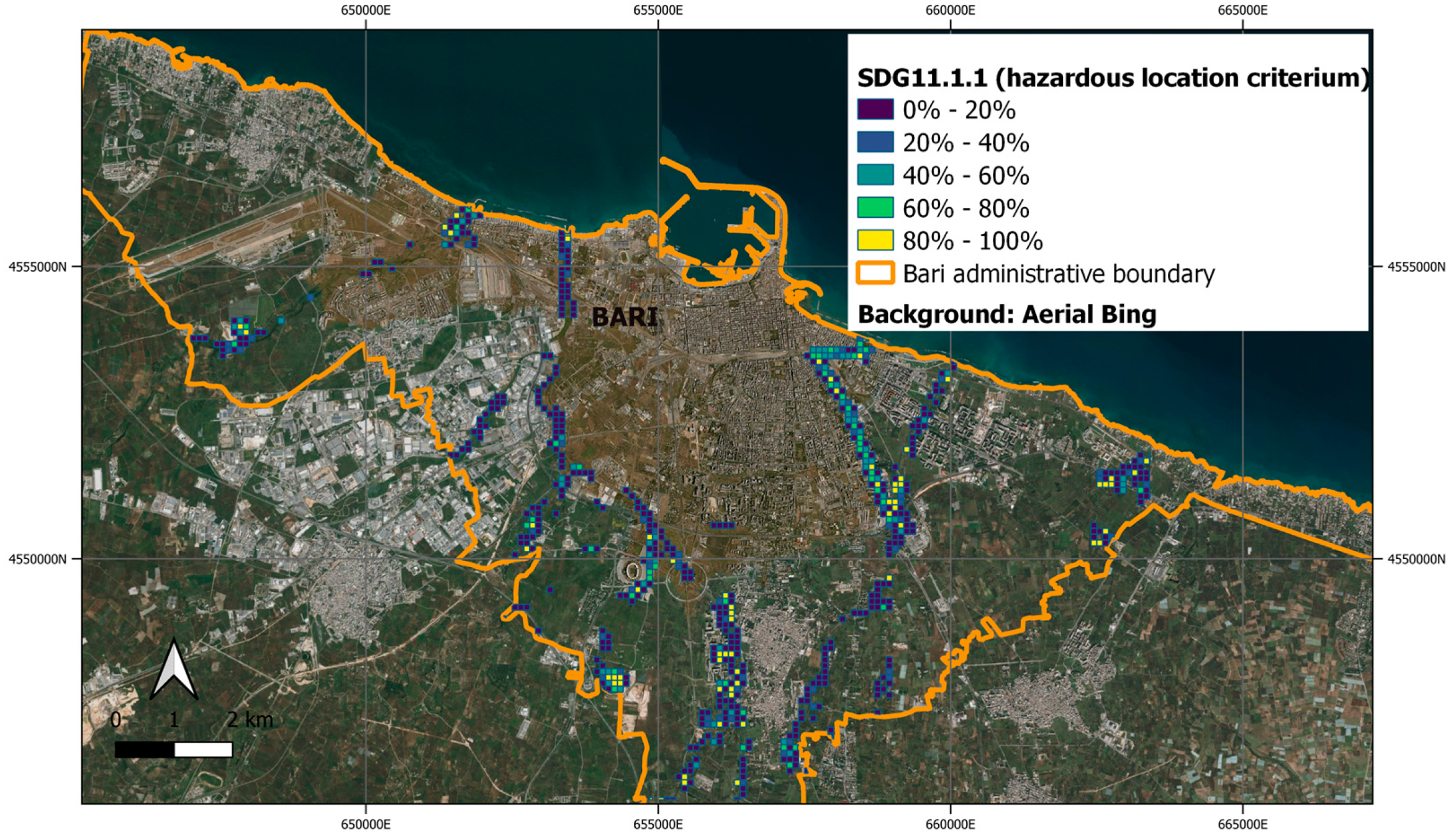
The map of areas subjected to flood hazard, Figure 6, was updated in November 2019 from the “Autorità di bacino distrettuale dell’Appennino Meridionale,” which was used as input for sub-indicator (2).
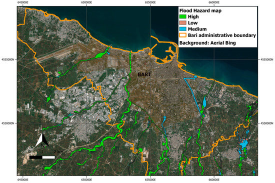
Figure 6.
Map of flood hazard in Bari up-to-date to November 2019. Source: “Autorità di bacino distrettuale dell’Appennino Meridionale”. Background source: Bing Aerial.
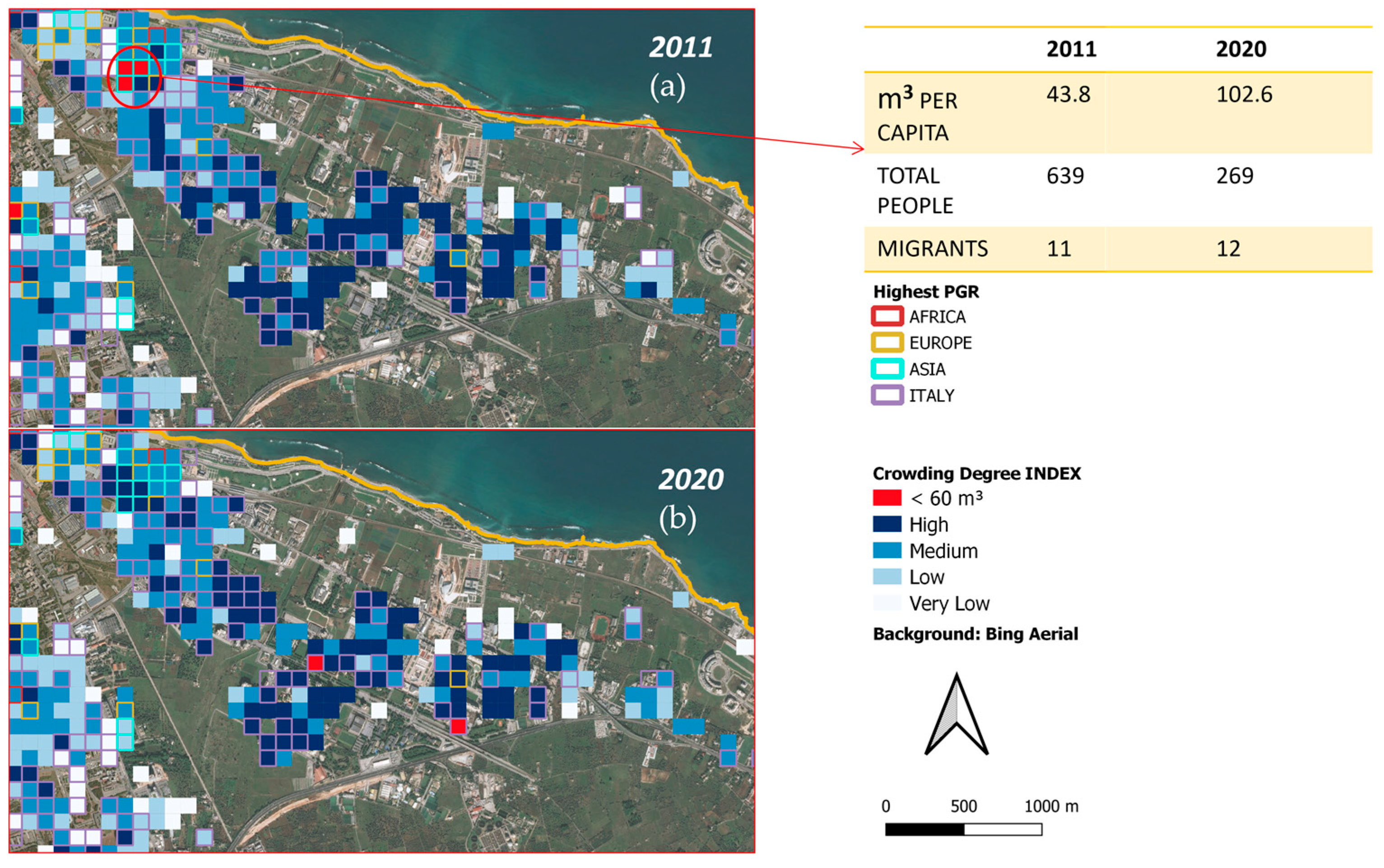
Sub-indicator (3) was introduced, in this work, as an additional criterion to define inadequate housing. To quantify the proportion of households with insufficient living space, building crowding degree maps were produced. The method to generate such maps consisted of calculating the housing per capita volume as a ratio between building volume and the number of resident people estimated in a cell. The analysis was performed using the 2020 and 2011 population grid maps and input data in Table 4. As depicted in Figure 7, LiDAR height data were combined with building layers to obtain a representative 3-dimensional model of buildings of the city. Thus, the volume was computed by multiplying the footprint areas with the mean value of heights for each building. The “civilario comunale” dataset (2017) was adopted as the latest update of the building layer. The settlement map from EO data was, instead, used as additional input to model the urban area in newly built neighbourhoods.
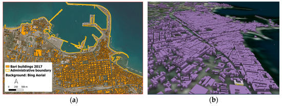
Figure 7.
Close-up from Bari municipality of: (a) building layer and (b) 3D model obtained by combining LiDAR and building layers.
As an inherent limitation of the methodology, the useful volume per inhabitant appeared to be overestimated, as it included floor thicknesses, walls and technical rooms of the buildings. The volume could also have been overestimated mainly in the central areas of the city, where buildings included many commercial spaces. The final classification of housing volume per capita was clustered into 3 categories of increasing degree of crowding: low, medium and high. This was carried out based on the results obtained. In addition, for a more detailed analysis of critical crowding values, a per capita volume threshold of 60 m3 was selected. As the useful height of a floor was approximately 3 m and the useful per capita volume was slightly overestimated, this threshold corresponded to less than 20 available square meters per capita. This threshold value conformed to the current legislation in Italy, according to which the limit criterion of habitability was about 14 square meters per inhabitant [32].
2.8. SDG 11.2.1 Indicator
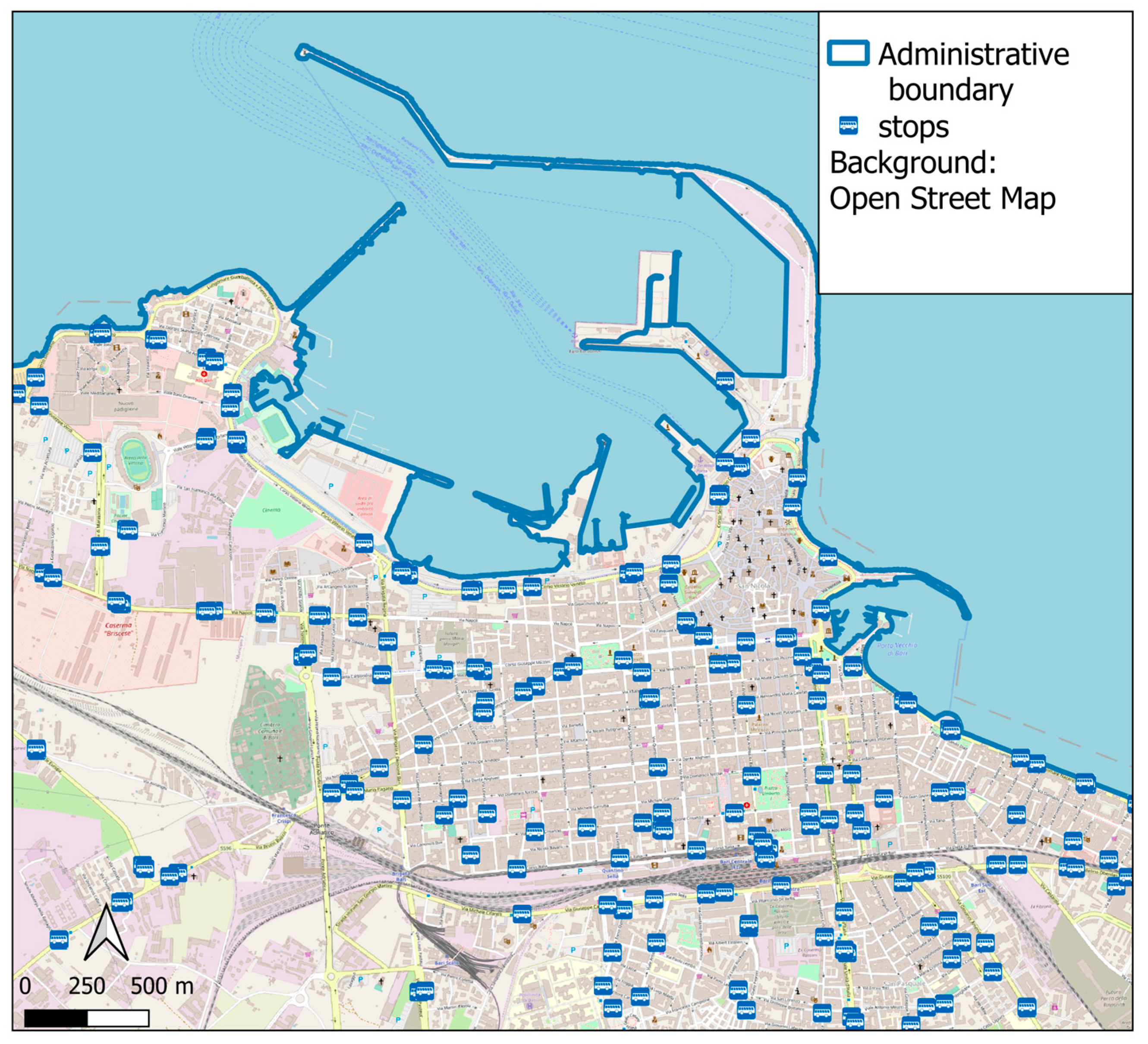
The SDG 11.2.1 indicator “Proportion of the population that has convenient access to public transport disaggregated by age group, sex and persons with disabilities” is, in this work, implemented for both the total and migrant populations. The methodology for calculating the indicator has been reported previously [33]. As main inputs, an inventory of public transport stops in the city and a network street graph were required. In this work, these layers were acquired from the open-data portal of Bari Municipality. A close-up bus stop map in Bari is depicted in Figure 8.
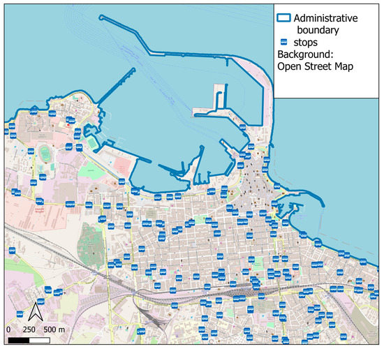
Figure 8.
Close-up of Bari bus stop map from Bari municipality open-data portal.
The metadata of indicators [33] suggested quantifying the proportion of the population that does not have convenient access to public transport by those who must walk more than 500 m to reach the nearest stop in the city. In this work, the fine-grid population density map was adopted as an input to evaluate indicators at both intra-urban and urban scales.
The processing chain, developed for this study, uses the PyQGIS libraries, designed for the analysis of network street graphs. The main steps of the implemented procedure are:
- The population grid is filtered by extracting those elements that do not contain one or more bus stops within;
- Each cell of the grid population density map is represented by its centroid;
- The centroids are projected onto the nearest point on the network street map which are denoted as starting points;
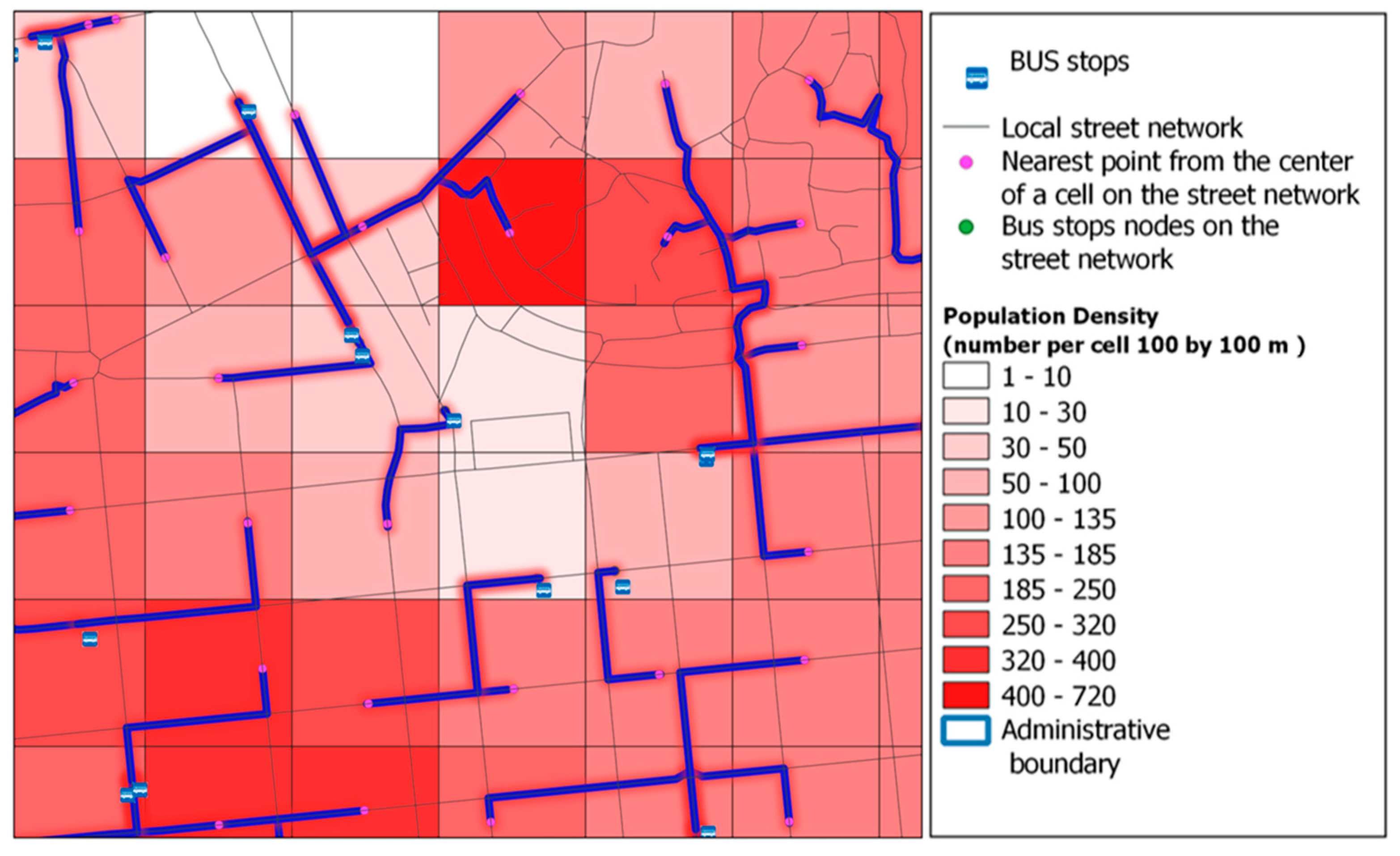
- Bus stops are also projected onto the nearest point on the grid which will be referred to as endpoints (Figure 9 provides a graphical representation of this step);
 Figure 9. Graphical representation of SDG 11.2.1. computation step 4. The walkable paths from starting to ending points are shown in blue.
 - For each starting point, an algorithm “graph tracker” searches for the nearest ending point, calculating the distance to travel necessary to reach it on the network;
- Those cells obtaining a distance greater than 500 m between starting and ending points are selected and highlighted.
The evaluation of indicators at the intra-urban scale consists of spatial overlapping of both total and migrant population density map with a spatial distribution map of the previously mentioned cells. The sum of the total population (including migrant component) living in these cells is an essential input to calculate the indicator at the urban scale.
2.9. SDG 11.3.1 Indicator
The formulas and procedures, for computing the SDG 11.3.1 indicator, have been described in [10]. The indicator was estimated according to its metadata description [34] already implemented in [10]. The related formula is based on the ratio between the Rate of Land Consumption (LCR) and the Population Growth rate (PGR) as follows
The only inputs required are the population data and settlement maps in two years). The former maps were obtained by applying the dasymetric method to population census data (dated 9 October 2011, and 1 January 2020, in this study). The latter map was obtained by downloading the European Settlement Map dated 2012 [35] and from the classification of 2019–2020 Sentinel-2 images. The ESM was based on satellite data acquired during 2011 and 2012. The temporal interval between the two considered epochs amounted to around eight years.
2.10. SDG 11.6.2 Indicator
According to the reference metadata [36], SDG indicator 11.6.2. “Annual mean levels of fine particulate matter (e.g., PM2.5 and PM10) in cities (population-weighted)” was implemented through spatially overlaying a population grid map (1 January 2020) with maps of the annual mean levels (2019) of atmospheric pollution from particulate matter (see input in Table 4). The latter data had a lower spatial resolution (4 km × 4 km) than the fine-grid population density map (100 m × 100 m). Thus, as suggested in [26], the indicator was aggregated at the urban scale using the formula
where
- is the city estimate;
- is the particulate matter concentration in a 4 km × 4 km cell;
- is population density value per cell 100 m × 100 m;
- is the number of cells of fine-grid population map included in a cell of atmospheric pollution map (4 km × 4 km);
- n is the number of cells of atmospheric pollution map covering Bari territory;
- is the total population of Bari.
3. Results
The results of the analysis consist of two parts. The former reports the results obtained for the input data for implementing SDG 11 indicators. The latter reports the 11 SDG indicators’ evaluation outcomes.
3.1. Input Data for Indicators’ Implementation
The first part of the results includes the classification map of a multi-temporal Sentinel-2 data set (Section 3.1.1), the weights adjustment factors for the new dasymetric method (Section 3.1.2), and the updated maps of total and regular migrant populations for both 2011 and 2020 (Section 3.1.3).
3.1.1. Settlement Map Updating and Land Consumption Rate
The updated settlement map (buildings only) was produced for 2020 from Sentinel-2 data. The map, shown in Figure 10, was obtained with an Overall Accuracy (OA) of 99.00% ± 0.33%.
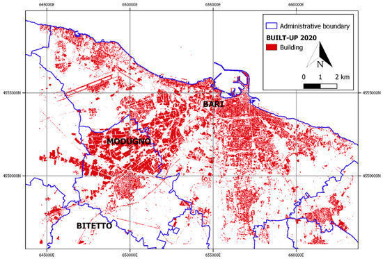
Figure 10.
Settlement map of Bari up to date to 2020 from SVM data-driven pixel-based approach.
For both the new settlement map (2020) and the reference ESM (2012), the building footprint area for each cell of the regular grid (100 m × 100 m) was estimated.
According to the methodology in [10], from these two maps, the Land Consumption Rate (LCR) component of SDG indicator 11.3.1 was extracted. The resulting output LCR map is shown in Figure 11. Values close to zero are representative of a stable state over time; positive values indicate an increase in artificial surfaces, and negative values represent a decrease in such surfaces. In most cases, as has been verified in [10], negative values are due to an overestimation of the artificial areas in the map of 2012 produced by [35].
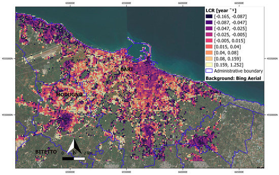
Figure 11.
Land Consumption Rate by comparing the settlement map up to 2020 with ESM 2012.
3.1.2. Weights and Adjustment Factors of the New Dasymetric Method
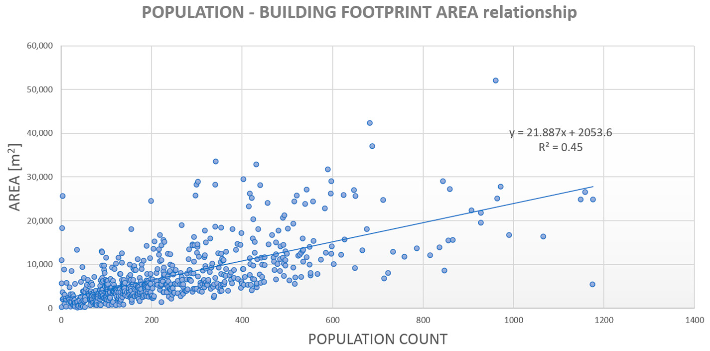
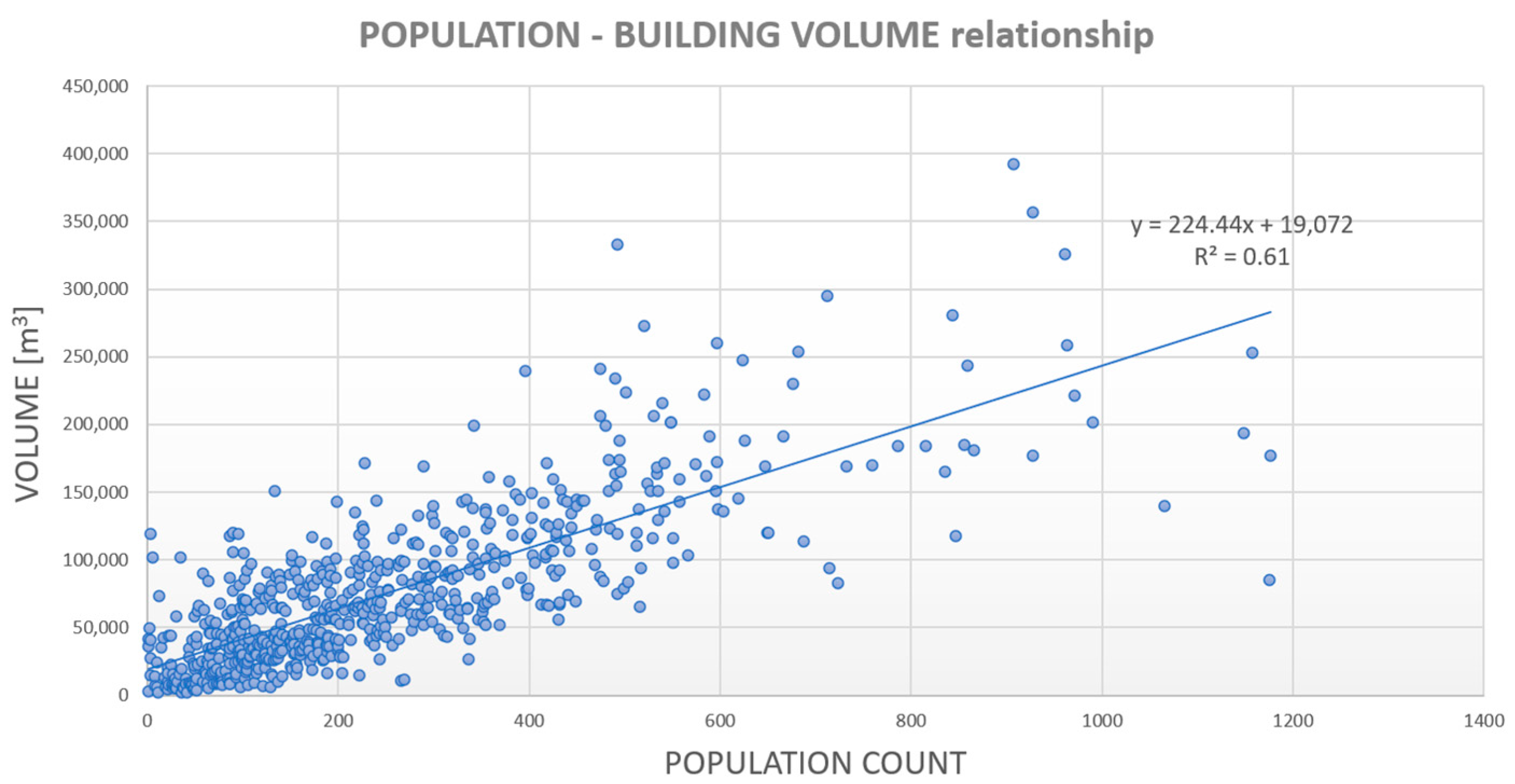
To evaluate the impact of building heights (and, thus, volumes) in the redistribution weights of the dasymetric method, a statistical analysis was carried out. Specifically, a linear regression of population density, first considering the footprint building area and, then, building volumes, was performed for about 600 census cells characterized mainly by residential building use (>90%), according to the UA layer (2018). The findings revealed that the correlation values between population and building footprint areas (R2 = 0.45) in Figure 12 were lower than those between population and volumes, reported in Figure 13 (R2 = 0.61).
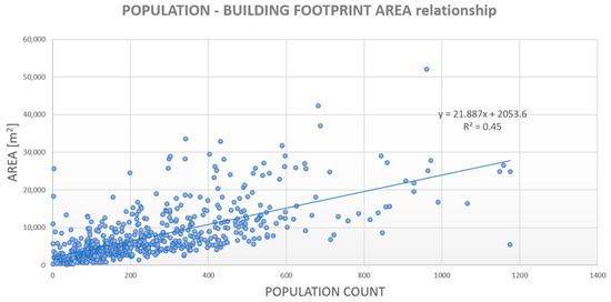
Figure 12.
Linear regression of Population against Building Footprint Area.
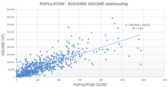
Figure 13.
Linear regression of Population against Building Volume.
In the case of census areas mainly used for industrial, commercial or other purposes, the population appeared not to be related to the volume of buildings. Industrial warehouses occupy large areas and are generally higher than a common floor of a residential building, even though they are not inhabited. Therefore, by comparing the average population density in non-residential areas (i.e., industrial, commercial, rural or others) with that in predominantly residential areas, correction factors for the weights were selected according to the building use. Consequently, these coefficients were, in this work, not fixed (like those used in [10,16]), but were site-specific. Table 5 reports the correction factor values per building use adopted in this study.

Table 5.
Correction factors per building use.
3.1.3. Regular Population Map Updating and Population Growth Rate
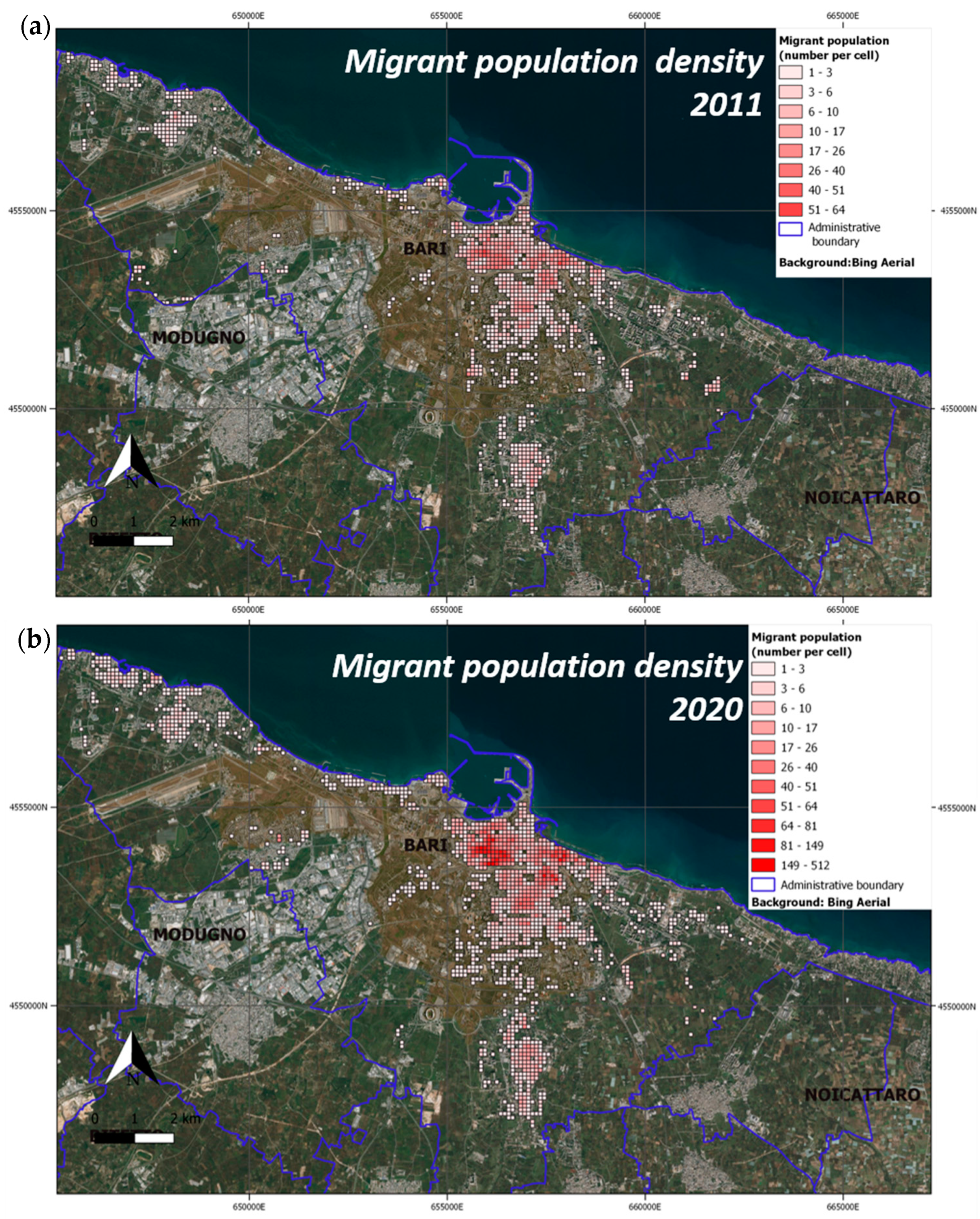
To obtain the fine-grid population map (100 m × 100 m), the building use data (Section 2.4), the settlement map (Figure 10) and the height-based weights from LiDAR sources were used as input to apply the dasymetric method to the population data by census zones (Section 2.3). The output maps for the total population and the regular migrant population are shown in Figure 14 and Figure 15, respectively.
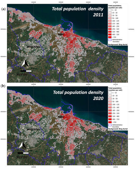
Figure 14.
Grid population density map for the total population in 2011 (a) and 2020 (b).
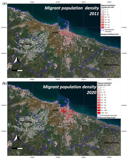
Figure 15.
Grid population map for migrant population component in 2011 (a) and 2020 (b).
For comparison, the classes in the choropleth representation [37] are the same in all images shown.
For accuracy evaluation, both the mean absolute error (MAE) and total absolute error (TAE) were used [10,27,38]. MAE and TAE values were used to verify that the aggregation of output cell data reproduced the total values associated with the original census areas [1]. The MAE value obtained over the 1291 census areas was 7 × 10⁻⁴, while the TAE value was 0.9 (number of people counted). This means that the final count of total persons after the application of the dasymetric method was close to the initial total number of persons. Compared to the migrant map, the errors obtained were on the same order of magnitude. As discussed in [27], the MAE was favoured as the main indicator of model performance, as opposed to the root mean square error (RMSE), because it appears more robust for a skewed distribution, as in the case of population density [38]; however, the RMSE was also computed to obtain a value around 10−3.
From the population density maps (Figure 14 and Figure 15), the Population Growth Rate (PGR) component of Indicator SDG 11.3.1 was extracted for both total and regular migrant populations. The output PGR maps obtained are shown in Figure 16.
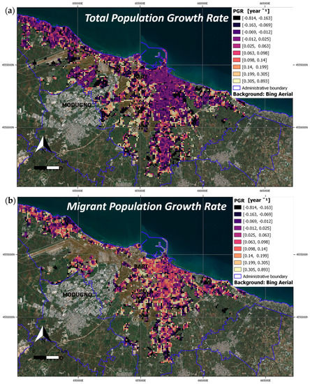
Figure 16.
Population Growth Rate from October 2011–January 2020, with respect to: (a) The total population; (b) the migrant population.
As depicted in Figure 16, the total and migrant populations had different patterns of expansion with a tendency for the migrant population to concentrate in the central area of Bari city. The native population, instead, seemed to prefer peri-urban areas where new residential districts had been built, such as the new south-eastern suburbs of the city. This finding confirms the results obtained in [10].
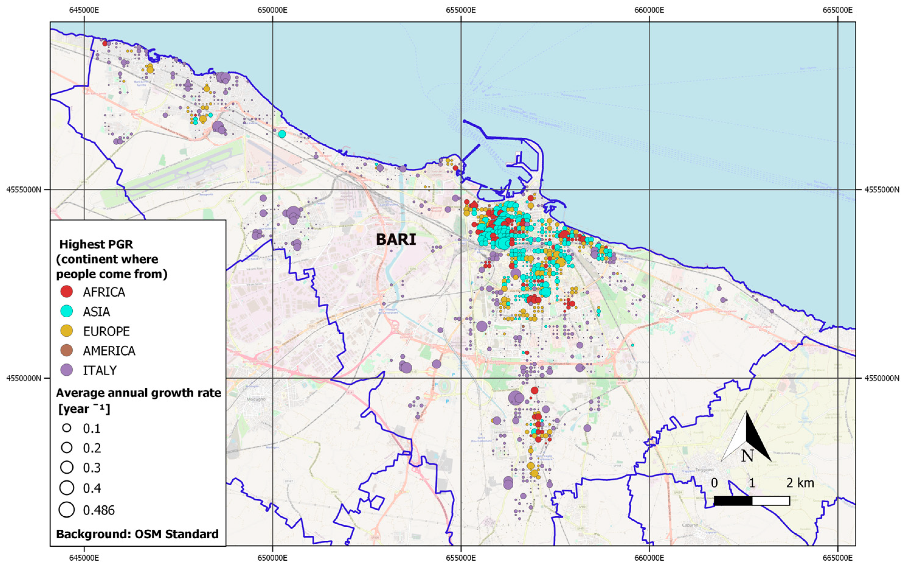
To provide information on both the spatial distribution of migrants, according to their continent of origin, and to identify the most significant elements contributing to population growth, the PGR indicator component was assessed by accomplishing disaggregation criteria for both local and migrant populations by continent. First, for each cell, the maximum PGR value (either positive or negative) was extracted and associated with the specific population category. Then, only positive maximum PGR values were filtered from the initial vectorial map to produce a new map (Figure 17). This map provides the spatial distribution of different population categories, as well as an indication of which categories had grown the most and where they had come from. In Figure 17, different colours are used to distinguish the different population components. The magnitude of the growth rate is represented with circles of increasing diameter.
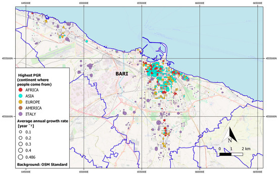
Figure 17.
Highest Population Growth Rate (positive increase).
Migrants from the Asian continent appeared to be dominant in the central area of the city. The most represented countries included Pakistan, Afghanistan, Bangladesh, Georgia and Iraq. Asiatic communities from China and the Philippines represented minorities in the southeast city residential areas. Although less numerous, African communities, mainly from Ghana, Somalia, Nigeria, Senegal, Gambia, Mali and Eritrea, overlapped with Asian groups. The non-Italian Europeans came mainly from Albania, Romania and Bosnia.
3.2. SDG 11 Indicators Evaluations
This sub-section includes the results obtained from the implementation of SDG 11 indicators: SDG 11.1.1 (Section 3.2.1); SDG 11.2.1. (Section 3.2.2); SDG 11.3.1 (Section 3.2.3); SDG 11.6.2 (Section 3.2.4). An additional Section 3.2.5 reports a summary of all proposed indicators at the urban scale. Section 3.2.6 is devoted to the uncertainty estimation.
3.2.1. SDG 11.1.1 Indicator
For indicator SDG 11.1.1, the population maps obtained with the new version of the dasymetric method were used as input to update sub-indicators (1) and (2) and to calculate the new sub-indicator (3), which was introduced in Section 2.8.
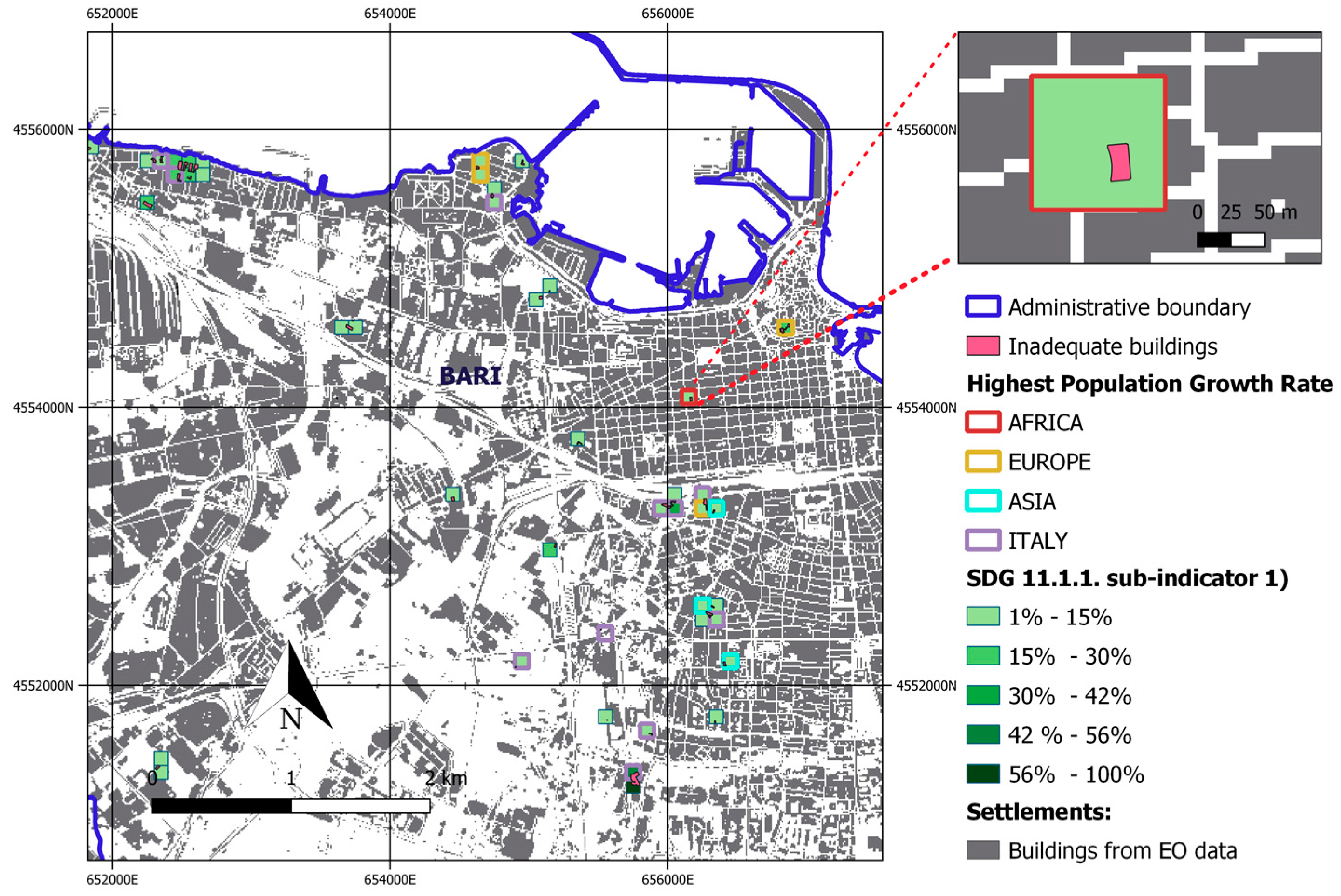
The map of sub-indicator (1) for SDG 11.1.1, updated for the total population in 2020, is shown in Figure 18. The total number of people living in areas with one or more inadequate buildings was 6151, of which 130 were migrants, even though only 596 people could potentially reside in such buildings. The latter number was based on both the proportion of inadequate buildings (from “civilario comunale” of Bari, 2017) to the total built-up area (settlement map updated to 2020) and the assumption that the population was uniformly distributed in the buildings. Many of these buildings are in central areas of the city, where there are positive growth rates of the regular migrant population from different continents. Unfortunately, it was impossible to verify whether people were living in the ruined buildings or in the adjacent ones (as each cell may contain both types of buildings). Such cases should, however, be highlighted to local authorities, as they are relevant to social inclusion issues.
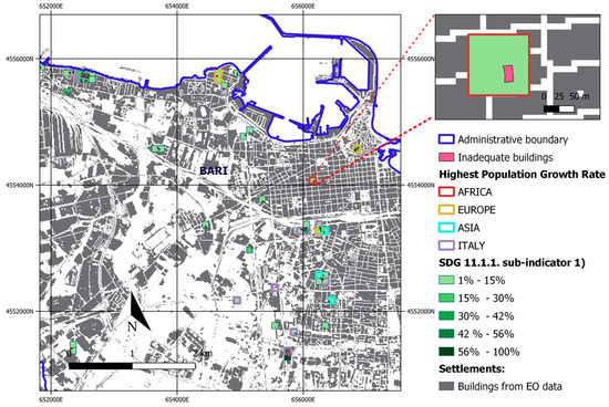
Figure 18.
SDG 11.1.1 sub-indicator (1) Proportion of households with non-durable housing.
The classes in the legend of Figure 18 define the percentage of people from a given cell potentially living in buildings with structural deficiencies.
The update of SDG 11.1.1 indicator (2) is shown in Figure 19. The total number of people living in the flood hazard areas in 2020 was approximately 3176 (or 1% of the total population); the estimated number of migrants was 133, or approximately 4% of the people living in the flood hazard area.

Figure 19.
SDG 11.1.1 sub-indicator (2) Proportion of households living in housing residing on or near hazardous areas.
As in Figure 18, the legend of Figure 19 provides the percentage of people potentially exposed to risk in each cell.
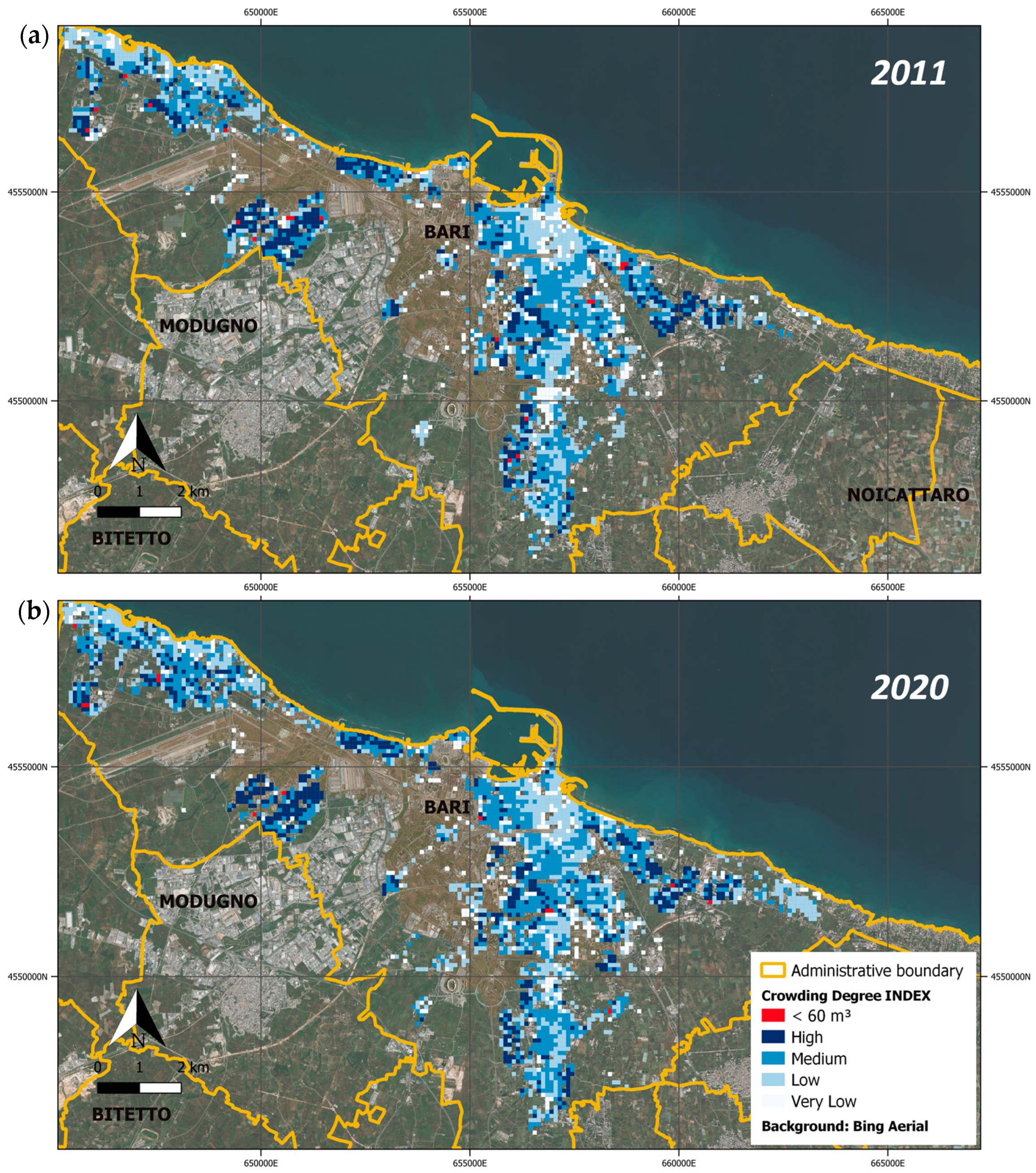
For the new SDG 11.1.1 sub-indicator (3), the housing volume per capita was estimated by multiplying the building areas by the heights from LiDAR data, then dividing the result by the number of people in each cell. The obtained map is shown in Figure 20.
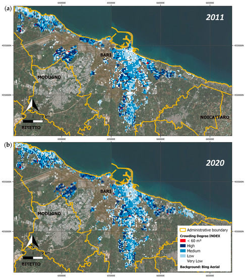
Figure 20.
SDG 11.1.1 sub-indicator (3). The proportion of households with insufficient living space from crowding degree map in (a) 2011, and (b) 2020.
It was observed that critical situations persisted in only a few elements of the regular grid. Thus, the intra-urban scale adopted for the calculation of the indicator appears to be an effective tool for identifying which urban neighbourhoods are most crowded, which grid elements are persistently overcrowded and which are those where the population is growing/declining.
For example, the San Paolo neighbourhood in the western suburbs of the city—which is already known for its state of urban and social decay—revealed increasing rates of the native population and a high degree of building occupancy. In the specific case examined (Figure 21), the per capita living area result was less than 8 square meters (below the regulatory limits [32]).
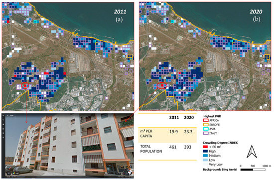
Figure 21.
Close-up of overcrowding degree map in St. Paolo District in: (a) 2011 and (b) 2020; specific building data (bottom).
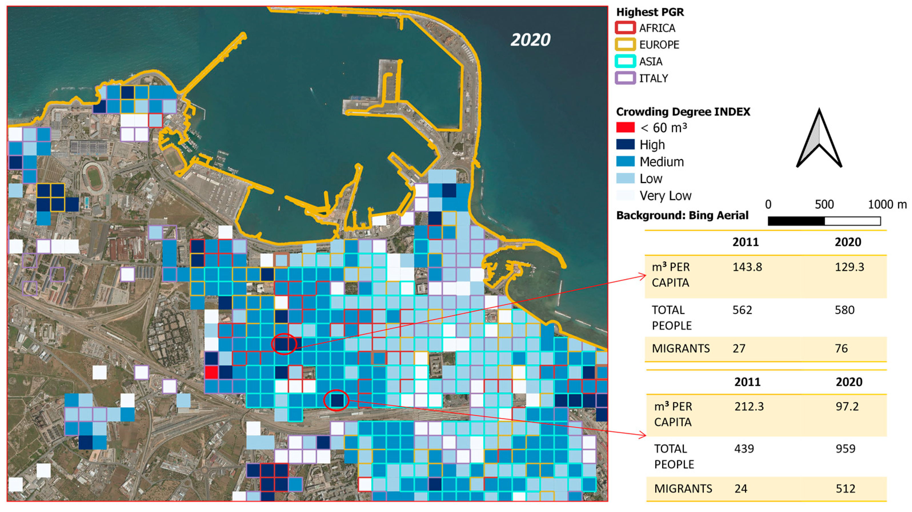
As an example of the increasing number of migrants settling in the central areas of the city, Figure 22 shows buildings occupied by migrants of predominantly Asian origin, from Pakistan, Afghanistan and Bangladesh.
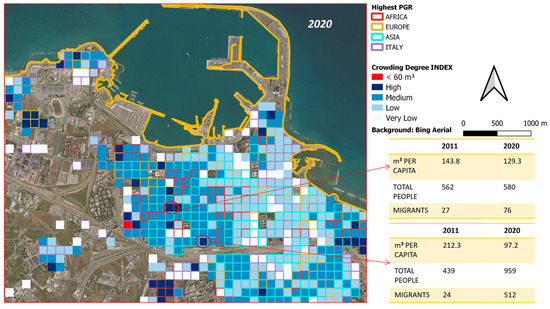
Figure 22.
Close-up of Bari central area: increasing crowding degree in some cells with highest migrant PGR.
As shown in Figure 23, some residential areas (e.g., Japigia district) appeared to be suffering from depopulation. These areas were close to a dismissed industrial area used as an asbestos fiber processing site in the past.
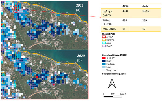
Figure 23.
Close-up of Bari residential areas close to old industrial abandoned areas, showing decreasing crowding degree between: (a) 2011 and (b) 2020.
3.2.2. SDG 11.2.1 Indicator
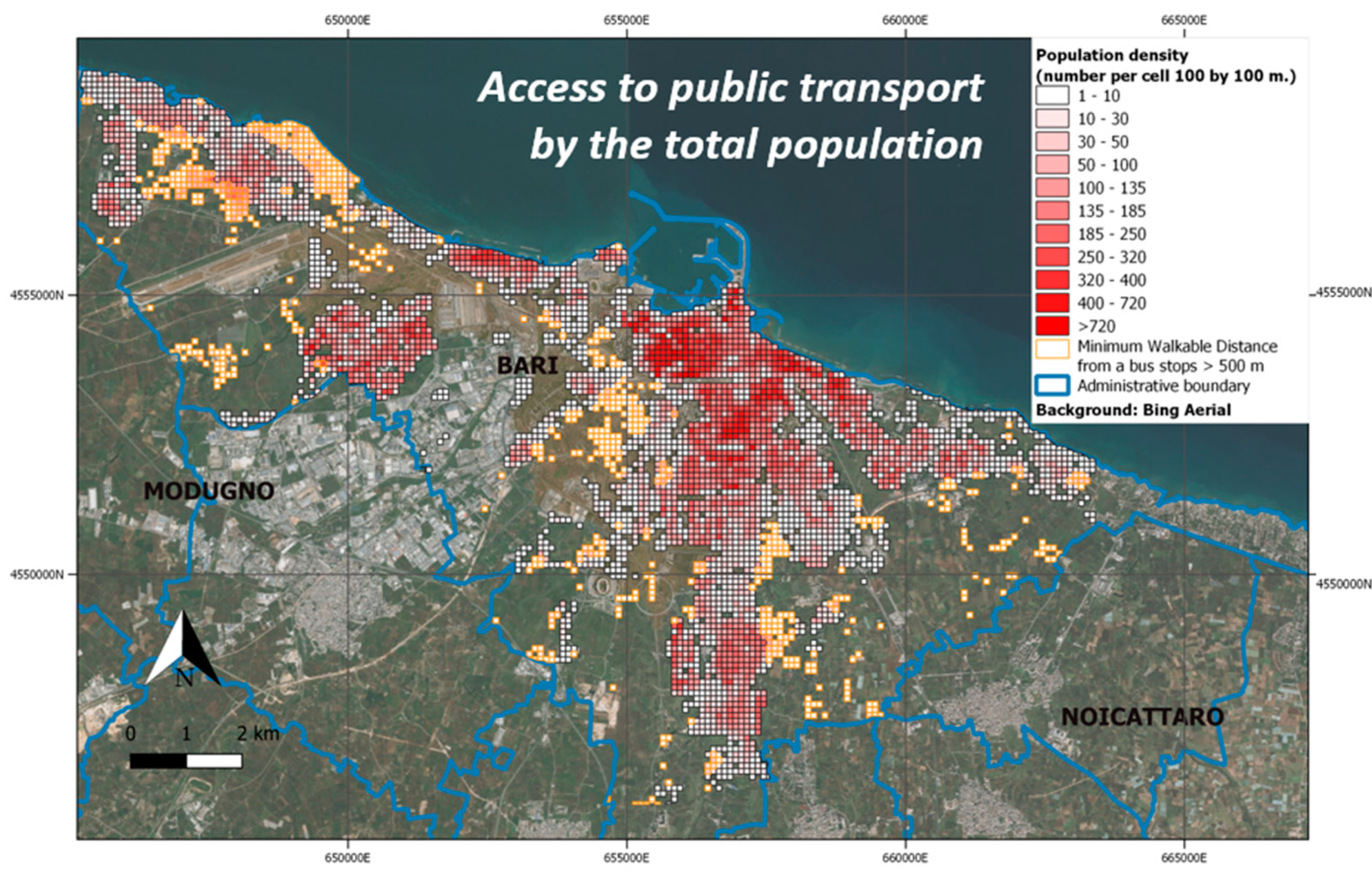
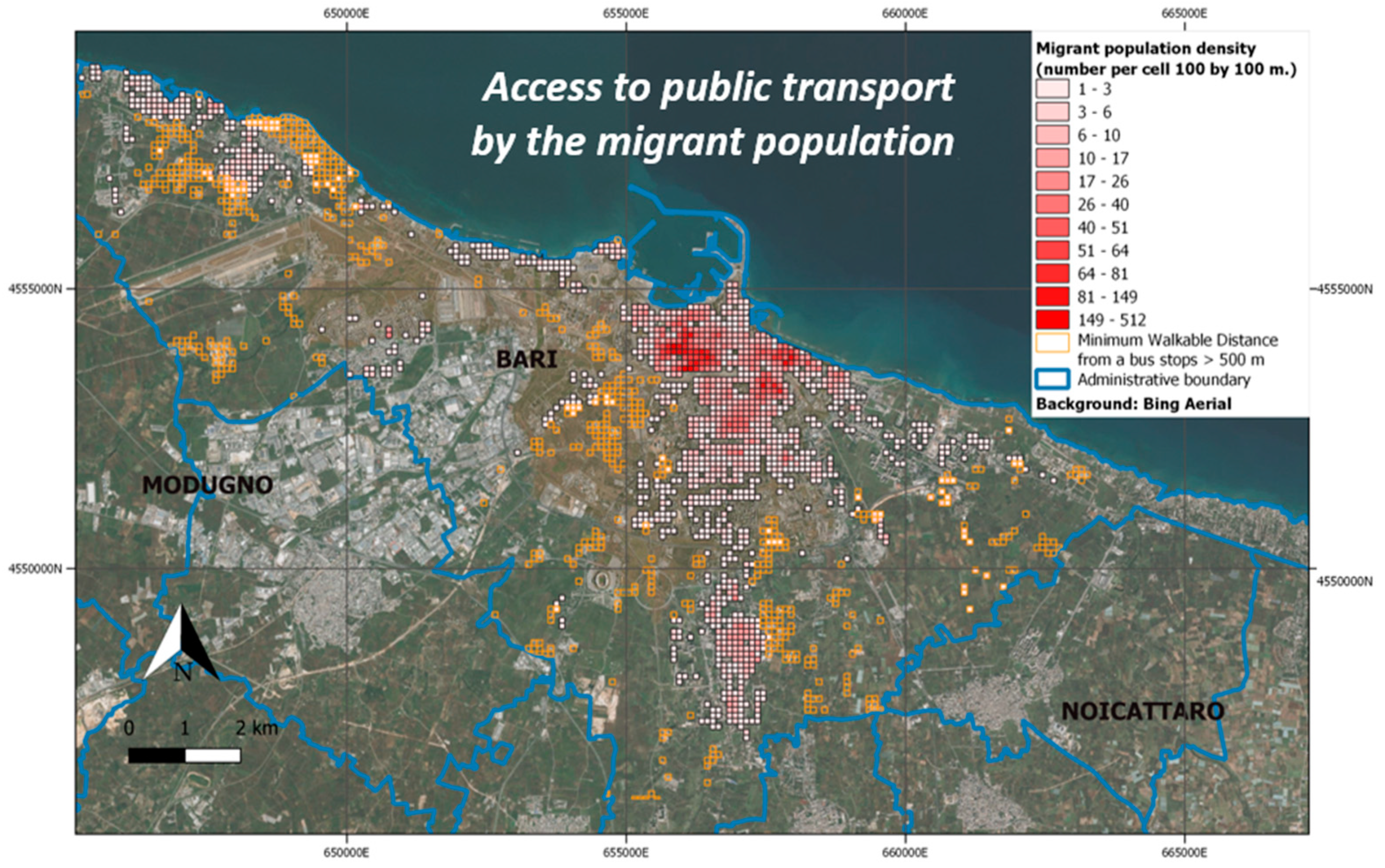
The SDG 11.2.1 indicator map is depicted in Figure 24 (total population) and Figure 25 (the migrant population component). The areas with orange colour were those where the population did not have easy access to public transportation, as they were more than 500 m away from the nearest bus stop. The estimated total was 10,135 people (about 3% of the total population); of these, only 226 people were estimated to be migrants. In general, from the maps, it appeared that access to services such as public transport results in a discriminating factor in the choice of settlements by migrant communities.
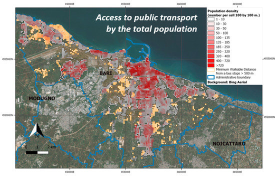
Figure 24.
SDG 11.2.1 Indicator: The cells in orange identify people that do not have convenient access to public transport as a proportion of the total population (including migrant component).
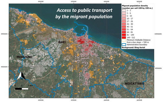
Figure 25.
SDG 11.2.1 Indicator: The cells in orange, identifying people that do not have convenient access to public transport, which do not overlap cells with high values of the migrant population density.
3.2.3. SDG 11.3.1 Indicator
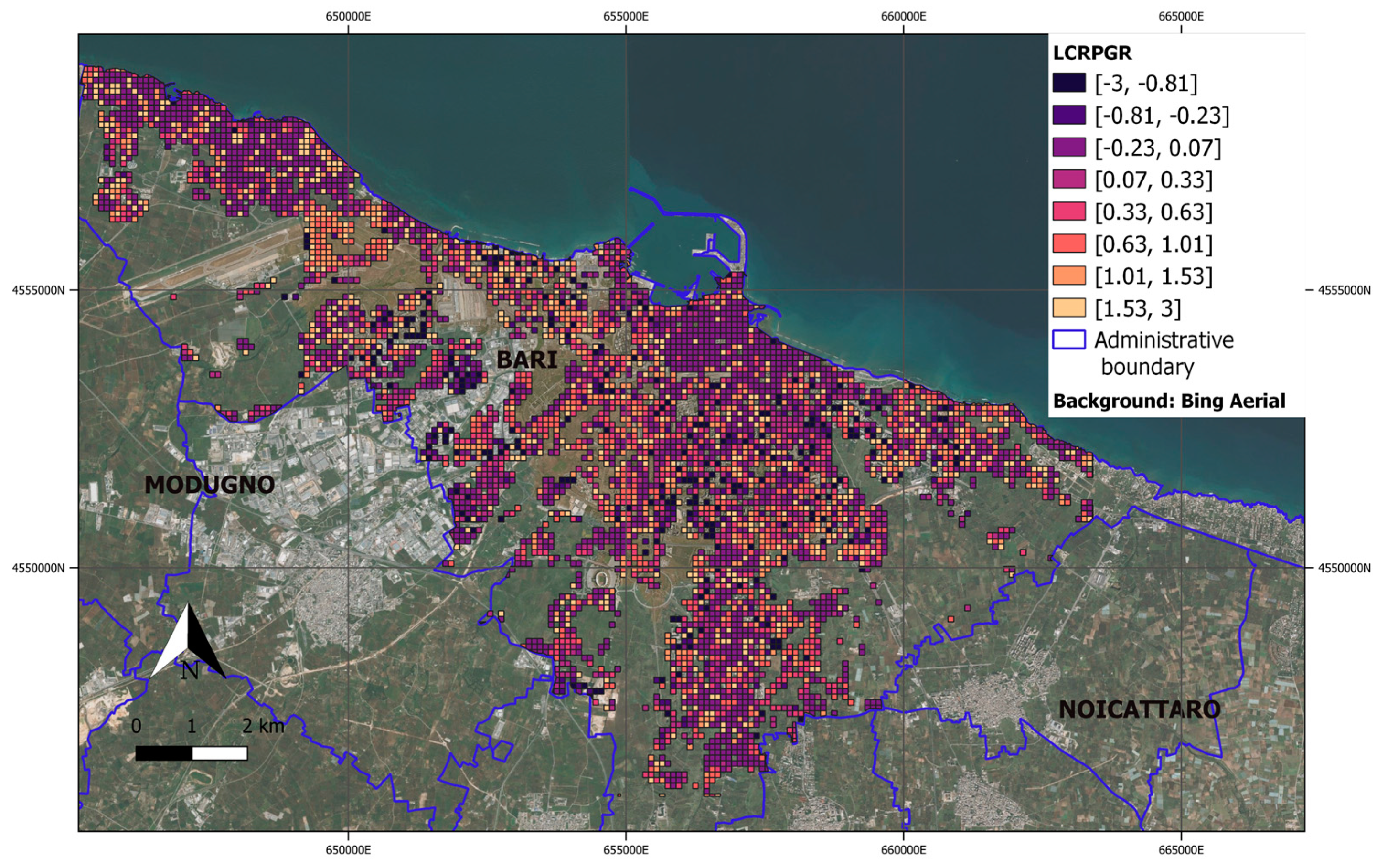
The indicator 11.3.1 “Ratio of Land Consumption Rate to Population Growth Rate” (LCRPGR) is known as “land use efficiency,” as it allows determination of where land consumption is justified by huge population growth and where, instead, it is due to external reasons such as industrial, commercial and tertiary expansion. As a novelty, in this paper, the PGR was evaluated for the total population (Figure 16a). The output product is shown in Figure 26.

Figure 26.
SDG 11.3.1 Indicator: LCRPGR.
Based on the ratio between LCR (Figure 10) and PGR (Figure 16a), very low positive values (violet tones) occurred in two cases:
- Very low LCR. This happened in consolidated urban areas such as the old town districts and other neighbourhoods (e.g., Murat);
- PGR was greater than LCR, such as in the central areas subjected to incoming migration flows.
Negative values mean that LCR or PGR was negative. Negative values of LCR were unrealistic scenarios, generally due to local errors in either the ESM (2011–2012) or the final (2020) settlement maps. As in [10], the ESM was found to have non-built areas erroneously labelled as buildings; as such, negative PGR values were due to internal population flows from some areas of the city to other areas. These flows may be due to environmental or economic factors, such as changes in the costs of apartments that were abandoned by the original resident population in those areas, as well as new religious facilities developed after 2011, such as a new mosque.
High values (orange-yellow colour) are dominant where LCR exceeded PGR; this suggests the presence of large areas subject to commercial, tertiary and industrial expansion.
3.2.4. SDG 11.6.2 Indicator
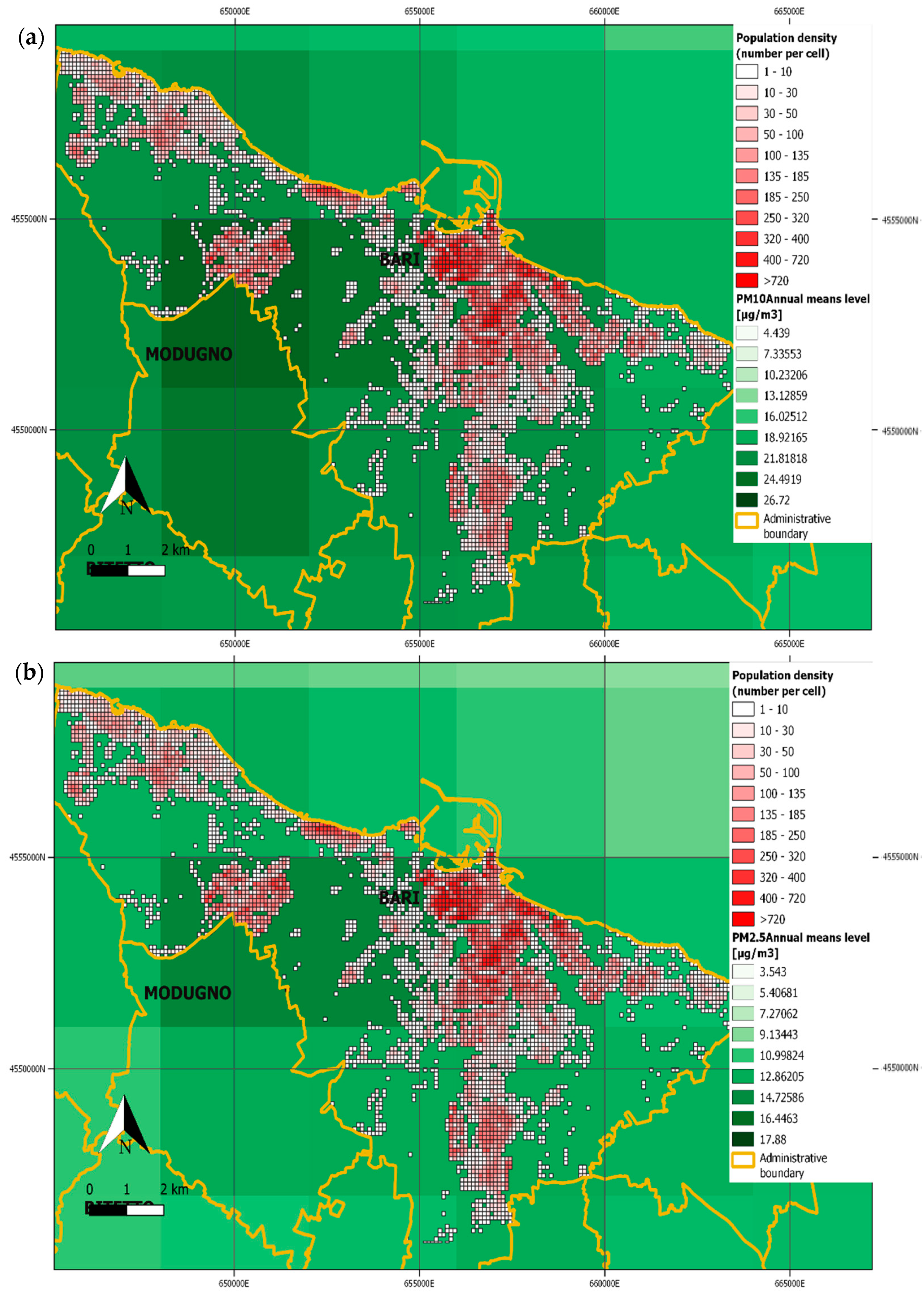
The SDG 11.6.2 indicator at intra-urban scale is depicted in Figure 27, showing a spatial overlay of grid population density map with air pollution information on the annual mean of particulate matter PM 10 and PM 2.5 maps.
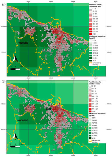
Figure 27.
SDG 11.6.2 Indicator: Annual mean levels of fine particulate matter weighted to total population of Bar city: (a) PM 10 and (b) PM 2.5.
According to the aggregation formula (2) at the urban scale (Section 2.10), the average exposure values, weighted to the total population, were 22.1 µg/m3 for PM and 13.5 µg/m3 for PM 2.5. Similar values were obtained when the pollution values were weighted to the migrant population component only. In both cases, the values were well below the legal limits for protecting human health; that is, 40 µg/m3 for PM 10 and 25 µg/m3 for PM 2.5 [39].
3.2.5. Evaluation of Indicators at Urban Scale
The SDG 11 indicators that, in previous sub-sections, were calculated and displayed as maps at the intra-urban scale are quantified in Table 6, as total/average values obtained. In other words, Table 6 reports the measures of SDG 11 indicators at the urban scale for Bari city.

Table 6.
Values of SDG 11 indicators obtained at urban scale for Bari city, for the total and migrant populations.
Such a table can be useful for comparative studies monitoring the progress toward the 2030 Agenda and New Urban Agenda across various cities.
However, in this study, the urban scale level was used to assess the primacy of the intra-urban scale in monitoring and informing about ongoing flows and processes, which were otherwise invisible when using a single value (Section 4.2.2).
3.2.6. Uncertainty Estimation
When assessing the uncertainties associated with the indicators, we assumed that they essentially depend on the uncertainty of the population density map produced by the dasymetric method. Such a map is the essential variable for indicator estimation.
The MAE, root mean square error (RMSE) and mean absolute percentage error (MAPE) were estimated at the output grid cell scale (100 m × 100 m).
A validation data set was created using the number of resident people, in the registry offices for each address. This data set was partly obtained automatically through geocoding tools in QGIS. However, some addresses were processed manually, due to the lack of a standardized toponymy data format.
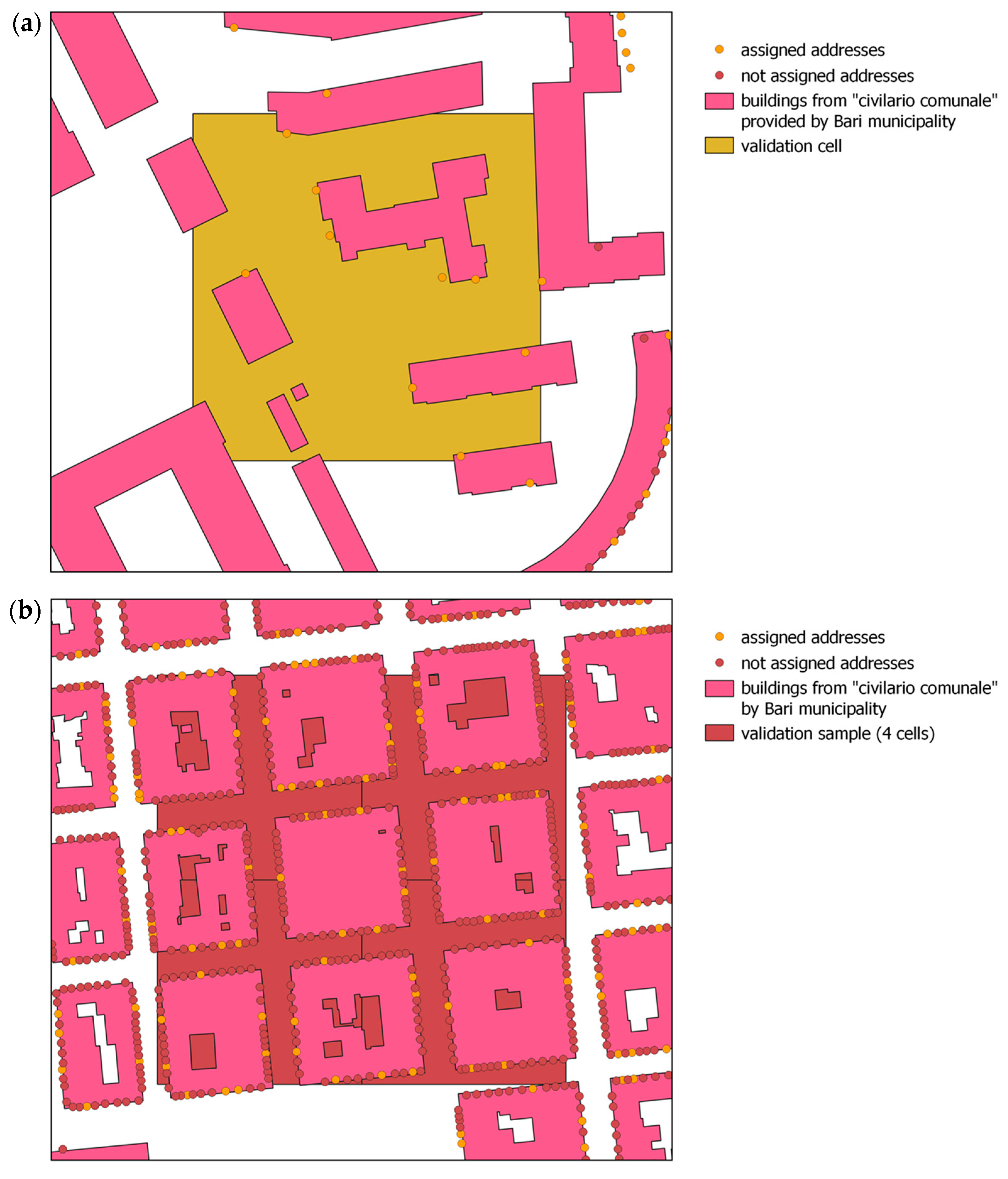
A further difficulty arose in matching house numbers (punctual data) to the corresponding buildings on the map, as the footprint area of the buildings could extend into more than one cell. The cells with the best match were selected for photo interpretation (see Figure 28). Validation samples sometimes considered a group of cells (Figure 28b), rather than just one cell (Figure 28a). In Figure 28 we denote the street numbers where we found resident people as “assigned addresses,” and those addresses where we did not find anyone as “not assigned addresses”. The uncertainty was estimated by comparing the number of residents registered at the addresses in the validation data sample () with the population data assigned to the cell by the dasymetric method ().
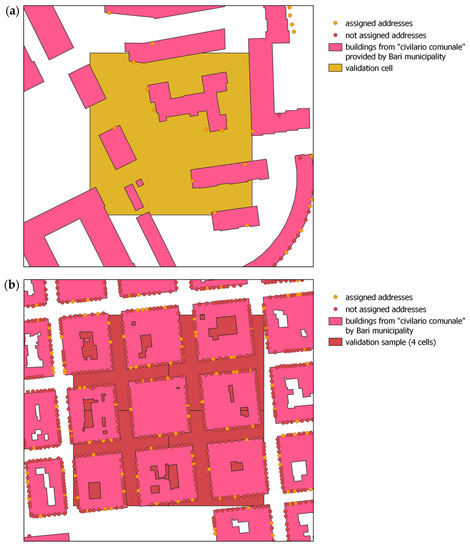
Figure 28.
Validation samples: (a) single cell; (b) group of cells.
The validation dataset was composed of 75 cells out of a total of 4821 (1.6%) non-zero cells. These cells were spatially well distributed and selected in order to ensure good spatial coverage with all indicator maps. The validation dataset was also used to evaluate the errors in the estimation obtained by applying the previous areal method [10], on the same population input data (2020). The achieved results are summarized in Table 7 and confirm the greater accuracy of the volume-based method implemented in this work.

Table 7.
Uncertainty estimations for the previous dasymetric mapping method [10] and the new improved method.
The ancillary input data (Section 2.6, Table 4, last column), used for calculating the indicators, were official products, issued by institutional authorities following long processes of verification and validation and after quality checking of the data. Therefore, we assumed that the usage of such data introduced negligible uncertainties. The methodologies implemented for calculating the indicators were the official methods included in the metadata [31,33,34,36].
4. Discussion
The present sub-section is articulated into two Section 4.1 and Section 4.2 focusing on the results obtained in Section 3.1 and Section 3.2, respectively.
4.1. Fine-Grid Population Map from EO and LiDAR Data
The allocation-of-population method presented in this paper belongs to hybrid Statistical–Dasymetric Modelling approaches [17]. The approach was dasymetric as, under its classical meaning, redistribution weights were defined based on information extracted from ancillary data. In this work, the building use maps derived from Urban Atlas and LiDAR-derived building height were used as new ancillary data compared to the previous method [10]. The approach was also statistical, as linear regression analysis (Section 3.1.2) was conducted preliminarily to identify and refine the redistribution weights.
As the main novelty of this study, the introduction of building height into the redistribution weights improved the population distribution depending on whether people resided in historical areas with buildings of up to three floors, in modern multi-floor buildings or villas/independent houses with 1–2 floors. Although [13] discussed the usefulness of building heights in demographic studies, and they implemented building volume estimation (from SAR data) as input for further applications, they did not apply such input to provide any output population density maps.
As a further innovation element for refining redistribution weights, the introduction of site-specific correction factors can lead to method standardization and reproducibility characteristics. These factors represent parameters for calibrating and adapting the method to the specific study area. Based on these two innovation elements, a high accuracy performance was achieved for the population density map with low TAE (0.9 number of people) and MAE (7 × 10⁻⁴ number of people) values (Section 3.1.3). The RMSE value obtained was about 10−3. The MAE and TAE values achieved by applying the previous version of the dasymetric method (based on building footprint area instead of volume [10]) were equally low but not negligible (the values obtained were 0.03 and around 40.81 number of people for MAE and TAE, respectively). This means that the final population count, after applying the previous dasymetric method, resulted in a deviation of around 41 units from the initial value. The RMSE value obtained was about 10−3 (number of people). This value was lower than the RMSE obtained from different LiDAR-based methods implemented and tested in [14], ranging from 0.25 to 0.75 (number of people). This difference may be because, in our paper, we derived the footprint area of the buildings, which are needed for volume evaluation, from the settlement map updated by EO satellite data (Sentinel-2) at 10 m resolution. Such updating can account for changes related to newly built areas, whereas the latest available Copernicus layer—namely, the European Settlement Map (ESM) Layer, 10 m resolution—was published in 2019, even though it was extracted from 2015 satellite data; however, the time lag that exists between satellite imagery acquisition and product validation/delivery cannot satisfy the rapid monitoring requirements of population flows (both migrant and native).
Concerning output population map validation, uncertainty evaluation is especially important for decision making applied to various fields, as discussed previously in [27,28,29,40]. However, data for such evaluation are rarely available and, even when available, they may exist at different periods or may interfere with confidentiality rules [17]. Based on the interaction with the local government and land management actors, the output maps obtained (2011 and 2020) seemed to be able to describe prior knowledge about trends in population and settlement transformation that had occurred in the city. A possible approach was presented in Section 3.2.6 and is discussed, hereafter, in Section 4.2.1.
As has already been highlighted in [10], the advantage of vector-based dasymetric methods, compared to raster ones, is that they can preserve all of the categories specified in the original database in the output database (i.e., age groups, gender and nationality). Such information can be used to easily monitor population flows and movements through space [41]. Considering the international scene, growing research activities focusing on complex interactions between human settlements and the environment have favoured the dissemination of methods and maps in a raster format, at a global scale [42,43]. These maps can support both the visualization of population rarefaction and concentration areas as well as providing counts of the total population residing in a specific study area; however, raster methods cannot provide information on the specific components (attributes) of a population.
4.2. Disaggregated SDG 11 Indicators
To the best of our knowledge, few studies have dealt with the implementation of SDG 11 indicators at the intra-urban scale. Thus, the discussion is articulated into two parts: The first deals with the still open research problem regarding the estimation of uncertainties associated with indicators; the second discusses the advantages of using the intra-urban scale to support decisions and government actions of local policy makers.
4.2.1. Uncertainty Analysis
To assess the uncertainties associated with the calculation of the indicators, in addition to considering the accuracy of the method at the level of census areas (Section 3.1.3), these were also addressed at the level of the elements of the grid (Section 3.2.6). This was because the indicators, on an intra-urban scale, were calculated at the resolution of the population grid (100 m × 100 m) and were also weighted to the population.
It is worth noting that the error value, based on reference in-situ data, was lower than that obtained through the old version of the dasymetric method (Section 3.2.6, Table 7). Nevertheless, as is well known, the collection of reference data for validation purposes is hampered by uncertainty and difficulties (Section 3.2.6). One of these difficulties is that not all statistical offices provide population and toponymy data in standard formats. Automatic tools are available in support of the geocoding of addresses, whose performance depends on the quality of the input data. When the data are available in the right format, the validation methodology can be easily reproduced.
As has been affirmed by [19,20], there are inherent uncertainties in population estimates which are difficult to eliminate. For example, the SDG 11.1.1 indicator aims to quantify people living in inadequate houses due to structural or sanitary deficiencies, overcrowding, or proximity to areas subject to natural hazards. However, such persons, in many cases, are not registered in the official population data statistics. Referring to the case of Bari, for example, homeless people as well as numerous irregular migrants were not included in the data used by this study. These people may improperly occupy abandoned or decaying buildings present in large numbers in historic districts. However, to date, no statistical data support this type of analysis. This has a direct impact on the estimation of the SDG 11.1.1 indicator and, indirectly, affects estimates of all indicators. The population living in urban areas, for these reasons, is inevitably underestimated [19,20].
The estimate of the error associated with the SDG 11.3.1, as it has been formulated, depends on the uncertainty of PGR estimate (at the scale of the grid population density maps) and that relating to the term LCR (obtained from the satellite-derived settlement maps). The nature of this latter uncertainty is twofold: On the one hand, the uncertainties depend on the performance of the automatic method (machine learning) to obtain the maps of settlements; on the other hand, the accuracy relates to the difficulty in obtaining a consistent semantic definition of built-up class in the implementation of the indicator [6].
In future developments, we intend to investigate uncertainty estimation issues, focusing on the implementation of automatic/semi-automatic procedures to expand the validation dataset.
4.2.2. Supporting SDG and NUA Policy Frameworks
The aim of the present work is to evaluate the impact of the proposed intra-urban scale implementation of indicators as innovation against the urban scale one. Based on the results obtained in the Section 3.2.5, such a large scale seems inadequate for implementing resilience policies, according to the SDG 11 framework and the NUA [4], in support of LRAs. For example, the average value of the SDG 11.3.1 indicator obtained (Table 6) indicated that the average land consumption rate, compared to demographic data, is increasing but remains lower than 1. When investigating at the intra-urban scale (Section 3.2.3), the land consumption rate value exceeded the unit in some grid cells (the yellow values in Figure 26) located, mainly, in the city peripheral areas. Thus, at the intra-urban scale, the indicator can identify the critical areas to be monitored due to excessive land consumption.
Based on such experience, the combined analysis of the results obtained at the intra-urban scale (Section 3.2.1, Section 3.2.2, Section 3.2.3 and Section 3.2.4), along with the evaluations at the urban scale (Section 3.2.5), can highlight ongoing processes and flows. Based on source [22], the total population of the study area has grown little over the last 20 years (about 2%), whereas the migrant population has increased (currently over 4% of the total) over the same period. Our analysis of the PGR indicator at the intra-urban scale carried out for both native and regular migrant components of the total population provided evidence that the two population groups are settling, according to different logics, in the existing urban fabric. The proximity to central areas where schools, hospitals and other services are present, as well as easier access to public transport (SDG 11.2.1 indicator), appears to favour the growth of migrant communities. In these central areas, the presence of poorly preserved buildings or building types with ground floors and attics that are improperly used for residential use is well-known to the local authorities (SDG 11.1.1 sub-indicator 1). In addition, deeper investigation of migrant’s PGR by continent revealed a tendency of people sharing a common language, culture and religion to aggregate in the same urban district. Native residents, instead, appear to have moved to the newly built residential areas of the suburbs.
Concerning the SDG 11.1.1 sub-indicator (3), in the central areas, based on threshold values used in this study (Section 3.2.1), there are currently no critical crowding values. In these areas, high PGR values of the regular resident migrant population were observed, e.g., in a cell of Figure 22, the number of people increased from 24 in 2011 to 512 in 2020. As evidenced in Section 3.2.1, the presence of commercial spaces in such areas could lead to an overestimation of the volume per capita and, thus, to an underestimation of the degree of crowding. Nevertheless, crowding could be higher due to the contribution of irregular migrants for whom no data are available. The results on SDG 11.1.1 sub-indicator (3) suggest focusing on densely populated areas in the western suburbs of the city, characterized by urban and social decay conditions experienced by the local population. In this suburb of the city, densely populated public popular houses are concentrated, but are not yet accessible to the migrant population.
The results for the indicator SDG 11.6.2 showed that the urban area affected by the highest air pollution by particulate matter was the industrial/commercial area in the southwestern suburbs of the city; however, there were no critical situations in the whole municipality [43].
5. Conclusions
The population density and distribution map on a 100 m × 100 m grid served as the fundamental input for constructing SDG 11 indicators. This paper provided a modification of the dasymetric method for the implementation of indicators at the intra-urban scale to support the choices of local policymakers and planners for the implementation of the goals of the 2030 Agenda and the New Urban Agenda.
The auxiliary input data used for Bari represent only one example of the types of data that need to be acquired for the implementation of indicators at the intra-urban scale. The diffusion of open databases serves as a promising prelude to the acquisition of data with the same information content, although in different formats, for other cities or geographical realities. The local dimension of the survey as well as the needs of the users cannot displace the necessity of acquiring these inputs by turning to local providers. The proposed modifications of the dasymetric technique can monitor flows of migrant and native populations over time, thus supporting the evaluation of their impacts on the progress of SDG 11 indicators. In addition, such knowledge about fluxes and processes can support the design and development of new policies and services aimed at fostering urban resilience and social inclusion. This is particularly true at a time when migration policies are being redefined at international level, as discussed in [44,45,46].
The methods can be implemented in different areas of interest. The authors, as future work, plan to apply the proposed approach to a different city: Reggio Calabria, southern Italy. Based on the preliminary work carried out, it is worth noting that the challenges related to the method implementation in a different area appear to mainly be related to a lack of input census data in standardized formats, the availability of updated LiDAR data and the availability of validation data (as well as the related confidentiality constrains). No additional issues can hamper the application of the proposed modified dasymetric method to other cities.
In future, work, to facilitate the exploitability, interoperability between models and reproducibility of the results, the dasymetric mapping module will be published using the Virtual Earth Laboratory (VLab) framework [47,48].
Author Contributions
Conceptualization, M.A. (Mariella Aquilino) and P.B.; methodology, M.A. (Mariella Aquilino) and P.B.; software, M.A. (Mariella Aquilino); validation, M.A. (Maria Adamo) and C.T.; formal analysis, M.A. (Mariella Aquilino), M.A. (Maria Adamo), C.T.; investigation, M.A. (Mariella Aquilino); resources, M.A. (Mariella Aquilino); data curation, M.A. (Mariella Aquilino); writing—original draft preparation, M.A. (Mariella Aquilino), C.T.; writing—review and editing, M.A. (Mariella Aquilino), C.T., P.B., A.B.; visualization, M.A. (Mariella Aquilino); supervision, P.B. and A.B.; project administration, P.B.; funding acquisition, P.B. All authors have read and agreed to the published version of the manuscript.
Funding
This research was funded by the project SMURBS—SMart URBan Solutions for air quality, disasters and city growth (www.smurbs.eu accessed on 4 December 2018) funded by the European Commission in the framework of program “The European network for observing our changing planet (ERA-PLANET)”, Grant Agreement: 689443 and by the OT4CLIMA project funded by the Italian Ministry of Education, University and Research (D.D. 2261 del 6.9.2018, PON R&I 2014–2020).
Institutional Review Board Statement
Not applicable.
Informed Consent Statement
Not applicable.
Data Availability Statement
Data sharing not yet available.
Acknowledgments
The authors are grateful to the following institutions for their valuable support: Demographic Services and Information Technology Offices of Bari municipality, “Autorità di bacino distrettuale dell’Appennino Meridionale”, and Regional Agency of Environmental Protection (ARPA Puglia).
Conflicts of Interest
The authors declare no conflict of interest. The funders had no role in the design of the study; in the collection, analyses, or interpretation of data; in the writing of the manuscript, or in the decision to publish the results.
References
- Ehrlich, D.; Kemper, T.; Pesaresi, M.; Corbane, C. Built-up Area and Population Density: Two Essential Societal Variables to Address Climate Hazard Impact. Environ. Sci. Policy 2018, 90, 73–82. [Google Scholar] [CrossRef] [PubMed]
- United Nations General Assembly (UNGA). Transforming Our World: The 2030 Agenda for Sustainable Development; United Nations: New York, NY, USA, 2015; Available online: https://www.un.org/sustainabledevelopment/sustainable-development-goals/ (accessed on 25 January 2020).
- Levarlet, F.; Celotti, P.; Alessandrini, M. A Territorial Approach for the Implementation of the SDGs in the EU—The Role of the European Committee of the Regions; Publications Office: Luxembourg, 2019; Volume 10. [Google Scholar]
- UN Habitat New Urban Agenda. United Nations Conference on Housing and Sustainable Urban Development (Habitat III) in Quito, Ecuador, on 20 October 2016. Available online: https://unhabitat.org/sites/default/files/2020/12/nua_handbook_14dec2020_2.pdf (accessed on 30 March 2021).
- Melchiorri, M.; Pesaresi, M.; Florczyk, A.; Corbane, C.; Kemper, T. Principles and Applications of the Global Human Settlement Layer as Baseline for the Land Use Efficiency Indicator—SDG 11.3.1. ISPRS Int. J. Geo-Inf. 2019, 8, 96. [Google Scholar] [CrossRef] [Green Version]
- Wang, Y.; Huang, C.; Feng, Y.; Zhao, M.; Gu, J. Using Earth Observation for Monitoring SDG 11.3.1-Ratio of Land Consumption Rate to Population Growth Rate in Mainland China. Remote Sens. 2020, 12, 357. [Google Scholar] [CrossRef] [Green Version]
- Stokes, E.C.; Seto, K.C. Characterizing Urban Infrastructural Transitions for the Sustainable Development Goals Using Multi-Temporal Land, Population, and Nighttime Light Data. Remote Sens. Environ. 2019, 234, 111430. [Google Scholar] [CrossRef]
- Shelestov, A.; Kussul, N.; Yailymov, B.; Shumilo, L.; Bilokonska, Y. Assessment of Land Consumption for SDG Indicator 11.3.1 Using Global and Local Built-Up Area Maps. In Proceedings of the IGARSS 2020—2020 IEEE International Geoscience and Remote Sensing Symposium, Waikoloa, HI, USA, 26 September–2 October 2020; IEEE: Waikoloa, HI, USA, 2020; pp. 4971–4974. [Google Scholar]
- Schiavina, M.; Melchiorri, M.; Corbane, C.; Florczyk, A.; Freire, S.; Pesaresi, M.; Kemper, T. Multi-Scale Estimation of Land Use Efficiency (SDG 11.3.1) across 25 Years Using Global Open and Free Data. Sustainability 2019, 11, 5674. [Google Scholar] [CrossRef] [Green Version]
- Aquilino, M.; Tarantino, C.; Adamo, M.; Barbanente, A.; Blonda, P. Earth Observation for the Implementation of Sustainable Development Goal 11 Indicators at Local Scale: Monitoring of the Migrant Population Distribution. Remote Sens. 2020, 12, 950. [Google Scholar] [CrossRef] [Green Version]
- Pesaresi, M.; Corbane, C.; Ren, C.; Edward, N. Generalized Vertical Components of Built-up Areas from Global Digital Elevation Models by Multi-Scale Linear Regression Modelling. PLoS ONE 2021, 16, e0244478. [Google Scholar] [CrossRef]
- Frantz, D.; Schug, F.; Okujeni, A.; Navacchi, C.; Wagner, W.; van der Linden, S.; Hostert, P. National-Scale Mapping of Building Height Using Sentinel-1 and Sentinel-2 Time Series. Remote Sens. Environ. 2021, 252, 112128. [Google Scholar] [CrossRef]
- Corbane, C.; Kato, S.; Iwao, K.; Sabo, F.; Politis, P.; Pesaresi, M.; Kemper, T. Leveraging ALOS-2 PALSAR-2 for Mapping Built-up Areas and Assessing Their Vertical Component. IEEE J. Sel. Top. Appl. Earth Obs. Remote Sens. 2020, 13, 6473–6483. [Google Scholar] [CrossRef]
- Pavía, J.M.; Cantarino, I. Can Dasymetric Mapping Significantly Improve Population Data Reallocation in a Dense Urban Area?: Dasymetric Mapping in an Urban Area. Geogr. Anal. 2017, 49, 155–174. [Google Scholar] [CrossRef]
- Copernicus Land Monitoring Services (CLMS). Urban Atlas (UA). 2020. Available online: https://land.copernicus.eu/local/urban-atlas (accessed on 30 March 2021).
- Alessandrini, A.; Natale, F.; Sermi, F.; Vespe, M. High Resolution Map of Migrants in the EU. JRC Tech. Rep. EUR 2017, 28770. [Google Scholar] [CrossRef]
- Leyk, S.; Gaughan, A.E.; Adamo, S.B.; de Sherbinin, A.; Balk, D.; Freire, S.; Rose, A.; Stevens, F.R.; Blankespoor, B.; Frye, C.; et al. The Spatial Allocation of Population: A Review of Large-Scale Gridded Population Data Products and Their Fitness for Use. Earth Syst. Sci. Data 2019, 11, 1385–1409. [Google Scholar] [CrossRef] [Green Version]
- Nagle, N.N.; Buttenfield, B.P.; Leyk, S.; Spielman, S. Dasymetric Modeling and Uncertainty. Ann. Assoc. Am. Geogr. 2014, 104, 80–95. [Google Scholar] [CrossRef] [PubMed] [Green Version]
- Kuffer, M.; Persello, C.; Pfeffer, K.; Sliuzas, R.; Rao, V. Do We Underestimate the Global Slum Population? In Proceedings of the 2019 Joint Urban Remote Sensing Event (JURSE), Vannes, France, 22–24 May 2019; IEEE: New York, NY, USA, 2019; pp. 1–4. [Google Scholar]
- Kuffer, M.; Wang, J.; Nagenborg, M.; Pfeffer, K.; Kohli, D.; Sliuzas, R.; Persello, C. The Scope of Earth-Observation to Improve the Consistency of the SDG Slum Indicator. ISPRS Int. J. Geo-Inf. 2018, 7, 428. [Google Scholar] [CrossRef] [Green Version]
- SVIMEZ. Il Mezzogiorno Nella Nuova Geografia Europea Delle Disuguaglianze. 2019. Available online: http://lnx.svimez.info/svimez/wp-content/uploads/2019/11/rapporto_svimez_2019_sintesi.pdf (accessed on 20 January 2021).
- ISTAT. Demographic Indicators. 2020. Available online: http://dati.istat.it/Index.aspx?QueryId=18462 (accessed on 30 March 2021).
- USGS Portal. Available online: https://earthexplorer.usgs.gov/ (accessed on 9 May 2018).
- Mountrakis, G.; Im, J.; Ogole, C. Support Vector Machines in Remote Sensing: A Review. ISPRS J. Photogramm. Remote Sens. 2011, 66, 247–259. [Google Scholar] [CrossRef]
- Di Gregorio, A. Land Cover Classification System: Classification Concepts and User Manual: LCCS; Food & Agriculture Organization of the United Nations: Rome, Italy, 2005; Volume 2. [Google Scholar]
- Congalton, R.G.; Green, K. Assessing the Accuracy of Remotely Sensed Data: Principles and Practices, 2nd ed.; CRC Press: Boca Raton, FL, USA, 2008; ISBN 978-0-429-14397-7. [Google Scholar]
- Batista e Silva, F.; Gallego, J.; Lavalle, C. A High-Resolution Population Grid Map for Europe. J. Maps 2013, 9, 16–28. [Google Scholar] [CrossRef]
- Calka, B.; Bielecka, E. Reliability Analysis of LandScan Gridded Population Data. The Case Study of Poland. ISPRS Int. J. Geo-Inf. 2019, 8, 222. [Google Scholar] [CrossRef] [Green Version]
- Mennis, J. Generating Surface Models of Population Using Dasymetric Mapping. Prof. Geogr. 2003, 55, 31–42. [Google Scholar]
- Municipality of Bari. Technical Building Regulations. 2020. Available online: https://www.comune.bari.it/documents/114869/648857/Adozione+Bozza+Regolamento+Edilizio/7a0aa429-072f-4aac-be76-3d6967656742%20 (accessed on 31 May 2021).
- UN Habitat. SDG 11.1.1. Metadata (2018 Release). Available online: https://unhabitat.org/sites/default/files/2020/06/metadata_on_sdg_indicator_11.1.1.pdf (accessed on 30 March 2021).
- Repubblica Italiana. Decreto Del Ministero Della Salute “Altezza Minima e Requisiti Igienico Sanitari Principali Dei Locali Di Abitazione”; Gazzetta Ufficiale, n. 190, Istituto Poligrafico e Zecca dello Stato: Roma, Italy, 1975. [Google Scholar]
- UN Habitat. SDG 11.2.1. Metadata 2020. Available online: https://unhabitat.org/sites/default/files/2020/06/metadata_on_sdg_indicator_11.2.1.pdf (accessed on 30 March 2021).
- UN Habitat. SDG 11.3.1. Metadata (2018 Release). Available online: https://unhabitat.org/sites/default/files/2020/07/metadata_on_sdg_indicator_11.3.1.pdf (accessed on 30 March 2021).
- Copernicus Land Monitoring Services (CLMS). European Settlement Map (ESM). Available online: https://land.copernicus.eu/pan-european/GHSL/european-settlement-map (accessed on 30 March 2021).
- UN Habitat. SDG 11.6.2. Metadata 2017. Available online: https://unhabitat.org/sites/default/files/2020/07/metadata_on_sdg_indicator_11.6.2.pdf (accessed on 30 March 2021).
- De Lorenzo, N.; Dugger, A. Choroplet Map. Esri, U.S. Census Bureau. 2012. Available online: https://www.arcgis.com/apps/MapJournal/index.html?appid=75eff041036d40cf8e70df99641004ca (accessed on 1 March 2020).
- Willmott, C.; Matsuura, K. Advantages of the Mean Absolute Error (MAE) over the Root Mean Square Error (RMSE) in Assessing Average Model Performance. Clim. Res. 2005, 30, 79–82. [Google Scholar] [CrossRef]
- Repubblica Italiana. Decreto Legislativo 3 Aprile 2006, n. 152 Norme in Materia Ambientale; Gazzetta Ufficiale, n. 88, Istituto Poligrafico e Zecca dello Stato: Roma, Italy, 2006. [Google Scholar]
- Yao, R.; Wang, L.; Huang, X.; Niu, Z.; Liu, F.; Wang, Q. Temporal Trends of Surface Urban Heat Islands and Associated Determinants in Major Chinese Cities. Sci. Total Environ. 2017, 609, 742–754. [Google Scholar] [CrossRef]
- Forman, R.T.T. Urban Ecology: Science of Cities; Cambridge University Press: Cambridge, UK, 2013; ISBN 978-1-139-03047-2. [Google Scholar]
- WorldPop Global 100m Population. 2018. Available online: https://www.worldpop.org/ (accessed on 30 March 2021).
- Center for International Earth Science Information Network (CIESIN), Columbia University. Documentation for the Gridded Population of the World, Version 4 (GPWv4), Revision 11 Data Sets; NASA Socioeconomic Data and Applications Center (SEDAC): Palisades, NY, USA, 2018. [CrossRef]
- ARPA PUGLIA Relazione Annuale Sulla Qualità Dell’Aria in Puglia Anno 2019. Available online: https://www.snpambiente.it/2020/07/03/relazione-annuale-sulla-qualita-dellaria-in-puglia-anno-2019/ (accessed on 30 April 2021).
- Marcil, S.; Sharon, J. Biden Presidency Is Likely to Deviate from Trump Administration on Foreign Policy, Climate Change, Race Relations; Indian Express: Noida, India, 2021. [Google Scholar]
- European Parliament Resolution of 19 May 2021 on Human Rights Protection and the EU External Migration Policy (2020/2116(INI)). Available online: https://www.europarl.europa.eu/doceo/document/TA-9-2021-0242_EN.html (accessed on 31 May 2021).
- De Trinidad Young, M.-E.; Wallace, S.P. A Window of Opportunity Is Opening to Improve Immigrant Health: A Research and Practice Agenda. Am. J. Public Health 2021, 111, 398–401. [Google Scholar] [CrossRef] [PubMed]
- Santoro, M.; Mazzetti, P.; Nativi, S. The VLab Framework: An Orchestrator Component to Support Data to Knowledge Transition. Remote Sens. 2020, 12, 1795. [Google Scholar] [CrossRef]
Publisher’s Note: MDPI stays neutral with regard to jurisdictional claims in published maps and institutional affiliations. |
© 2021 by the authors. Licensee MDPI, Basel, Switzerland. This article is an open access article distributed under the terms and conditions of the Creative Commons Attribution (CC BY) license (https://creativecommons.org/licenses/by/4.0/).


