Article

Design of a Generic Virtual Measurement Workflow for Processing Archived Point Cloud of Trees and Its Implementation of Light Condition Measurements on Stems

1
Department of Earth Observation, Friedrich-Schiller-University Jena, Grietgasse 6, 07747 Jena, Germany
2
College of Material Science and Engineering, Beijing University of Chemical Technology (BUCT), Beijing 100029, China
3
Techniques Developing Department, National Engineering Research Center of Surveying and Mapping, Beijing 100039, China
4
School of Soil and Water Conservation, Beijing Forestry University, Beijing 100083, China
5
School of Forestry, Beijing Forestry University, Beijing 100083, China
*
Author to whom correspondence should be addressed.
Both authors contributed equally to this work.
Remote Sens. 2021, 13(14), 2801; https://doi.org/10.3390/rs13142801
Submission received: 13 March 2021 / Revised: 12 June 2021 / Accepted: 13 July 2021 / Published: 16 July 2021
(This article belongs to the Special Issue Terrestrial Laser Scanning of Forest Structure)

Abstract

:
Virtual measurement workflow (VMW) was a generic data mining method developed in this study. It was used to extract tree information from archived point clouds under limited conditions by applying virtual measurements in virtual reality. As an example of how to use VMW for a specific topic, the VMW implementation of light condition measurement was further developed. This implementation could measure the temporal and spatial distribution of sunlight on virtual trees (stems). The output was expected as a new type of raw measurement data for tree morphology and phycological studies. At a single tree scale, it facilitated the quantitative interpretation of the growth strategy of branches. By measuring a single tree, it was found that only 4.34% of the stem surface could be illuminated throughout the day (8 h). Meanwhile, 35.87% of the stem surfaces were exposed to sunlight for less than one hour a day. A further mathematical processing of the output, i.e., γ (a ratio between relative area of triangles and relative quantities of triangles in each exposure duration group) improved the sensitivity of identifying differences in lighting conditions. Furthermore, we measured virtual trees of four species from an additional data source using a standardized setting. These include the sessile oak, gemu tree, Masson’s pine, and cherry tree. It was found that the shape of the crown was also significant for the distribution of solar energy on stems. For instance, the gemu tree had a cylindrical tree crown with narrow tree skeleton. A percentage of 10.38 of the surface on the gemu tree was illuminated throughout the day (8 h). The Masson’s pine had similar height and DBH with the gemu tree. However, the elliptical tree crown of the Masson’s pines prevented more lights. The area on the stem that was exposed to sunlight (8 h) dropped from 10.38% to 5.71%. This good differentiation of different crown structures might help this VMW implementation to continue to develop as a tool for identifying the effect of various crown shapes on radiosity for different tree species. The successful development of this VMW implementation had several practical applications for tree studies. Meanwhile, it demonstrated the overall feasibility of VMW and provided a paradigm for further development of other VMW implementations.

1. Introduction

1.1. Difficulties in the Reuse of Point Clouds

Since the wide application of terrestrial laser scanning (TLS) was applied in forest sample plots, a large amount of point clouds was generated as raw data [1]. However, a lot of data were sealed after their initial tasks were completed. From the perspective of data mining, each archived point cloud is a treasure trove of tree information. As time passed, archived point clouds would be the only sources of data that preserve detailed information about the tree geometry at single tree level. This information would facilitate us to investigate the historical condition of trees. Compared to “real-time” workflows, the data mining on archived point clouds encounters two major difficulties. We summarized them as dependence and instantaneousness of point clouds.
Dependence of point clouds indicates that some tree parameters, e.g., diameter at breast height (DBH) and biomass, derived from point clouds have to be validated and calibrated using additional methods and reference [2]. This is because the growth of a tree is affected by many factors, such as climatic conditions of the landscape, quality of soil conditions, and biotic conditions [3,4]. Therefore, it is not easy to use standardized parameters to adapt to all the variations. Thus, auxiliary methods and references are widely applied to provide calibration and validation [5,6,7]. When performing data mining on an archived point cloud, the acquisition of auxiliary data becomes challenging.
Instantaneousness of point clouds refers to the temporal characteristics of TLS scanning. From our perspective, a point cloud is a freezing of the geometry of trees at a specific time. Each point cloud has a unique timestamp, which results in a problem in collecting new complementary measurements on the original sample plots. This temporal inconsistency between the archived point cloud and new complementary measurements seems to be an irresolvable contradiction.

1.2. Development of the Virtual Measurement Workflow (VMW)

According to the aforementioned difficulties in the reuse of point clouds, two specific prerequisites for data mining were clearly known to us. Primarily, the archived point cloud would be the only data source. Secondly, new complementary measurements had to have the same timestamp of the archived point cloud. In accordance with these two requirements, we developed the virtual measurement workflow (VMW) in this study.
VMW was a workflow that consisted of three processes. The first process was the original TLS scanning, which produced the original (archived) point cloud. The second process was the shift of measuring target. In this process, the measuring target would change from real trees in nature to virtual trees in virtual space. Then, in the third process, virtual trees would be measured using Computational Virtual Measurement (CVM) as the simulation of applying complementary measurements at the original moment. CVM was the virtual measuring method developed in this study. CVM simulated natural physical laws in virtual space as a virtual measurement instrument (VMI) to measure virtual trees. Fundamentally, CVM was a measuring process without mathematical predictions. Thus, applying a CVM process was similar to using a real measuring instrument in reality.
VMW was a generic methodology. The use of VMW for a specific purpose was called VMW implementation. To provide a practical example of how this worked, we implemented the VMW for assessing the light condition of a single tree stem using an archived point cloud. The original TLS scan was a general scan of a university campus without a specific purpose on tree parameters estimation.

1.3. Conventional Methods of Assessing Light Condition in Sample Plots

In nature, light is the primary energy source for plant growth. A lot of biological activities for plants directly rely on light conditions, e.g., photosynthesis and transpiration [8,9]. Competition for a better light condition is a common growth strategy for individual trees by extending canopy structures in vertical and horizontal directions [10]. Therefore, the quantitative assessment for light conditions is preferential for studying tree biology.
Radiation detection is the dominant method for assessing light conditions in forests [11,12,13]. In a forest field, the light intensity is usually recorded by quantum sensors [14]. Photosynthetic photon flux density (PPFD) is the quantitative indicator for light conditions [6]. The measuring for PPFD above canopies is straightforward because shading effects do not exist. On the contrary, the distribution of sensors under a canopy has a great influence on the value of PPFD due to uneven tree shades [15]. Moreover, for a single tree in forests, radiation sensors cannot distinguish interference from surrounding objects, e.g., adjacent trees, tall grass, and bushes. In the meantime, the sensor readings are affected by many environmental variables, e.g., the date, clouds, air humidity, and wind [16].
By including radiation detection, several measuring methods can provide general indications for light conditions of a single tree. We divided those methods into two groups: direct and indirect. The direct methods provide the natural characteristics of the targets. One kind of measurement is based on crown morphology [17]. The conventional dendrometric description for crown shapes is facile. Regular shape objects such as cones and semi-spherical balls are used to represent tree crown [18]. Allometric relationships between tree height (H) and diameter at breast height (DBH) are used to create tree crown models [19]. Some studies include crown width in their modeling process [20,21]. With the development of light detection and ranging (lidar), highly precise estimations for crown shapes are available [22,23]. Canopy gaps are also a significant indicator of light conditions [24,25]. However, its scope is usually for multiple trees in the forest. Different from the methods for crown (canopy) measurement, the leaf area index (LAI) is recognized to be better for single tree analysis [26,27]. LAI is the total one-sided area of leaf tissue per unit ground surface area [28]. LAI is an allometric method, which connects the area with the capability of photosynthesis for leaves. Meanwhile, LAI is characterized as a systematic sampling method [29].
In addition to the direct measurements, indirect methods can be used to evaluate light conditions by measuring the metabolites of trees [30]. At the leaf level, canopy photosynthesis and transpiration measurement system (CAPTS) is utilized to measure and describe the intensity of photosynthesis by indirectly using CO2 uptake rates [31]. However, it is labor-intensive work for a single tree [32].

1.4. Assessing Light Condition Using VMW

Due to the inconsistency of the timestamps, we were unable to perform any additional measurements on the original sample plots. Before CVM was applied to simulate the physical processes of real measurement instruments, it was necessary to design feasible simulation scenarios. Due to the capabilities of computer hardware and software, the exact reproduction of natural measurement was difficult to achieve. Therefore, we summarized different measuring methods for assessing light conditions in Table 1 in order to find a feasible physical scenario in virtual spaces.
According to the measuring duration, conventional methods could be divided into two groups: instant and continuous. The instant group indicates the measuring instruments taking information on targets instantly, e.g., Lidar scanning [33] and leaf area measuring [34]. The continuous group refers to the fact that measuring instruments continuously gather information on targets, e.g., some of the radiation recordings [13] and metabolites detecting [35]. It is well known that the positions of the sun vary at each moment during daylight. Thus, continuous measurements perform better than instant measurements for recording natural light conditions.
Finally, a feasible CVM process was developed to provide information on the temporal and spatial distribution of solar energy on stem surfaces of a single tree. This process integrated a few features in Table 1. There were (i) direct feature; (ii) the feature of targeting irradiation and tree together; (iii) continuous feature; (iv) the feature of no systematic or allometry. The measuring output was a 3D mesh. Temporal and spatial distribution of solar energy was recorded in each triangle in this 3D mesh. This output consists of raw measuring data, such as tree height and DBH. It was not bound to a specific study topic. Methods for utilizing this kind of data were demonstrated.

2. Materials and Methods

2.1. Development of Virtual Measurement Workflow (VMW)

2.1.1. Missions and Features of VMW

The development of virtual measurement workflow (VMW) was the essential aim in this study. VMW aimed to extract tree/forest information from archived data sources (point clouds in this study). It was a workflow toward data mining and data utilization. Due to previous introduced difficulties in the reuse of point clouds (in Section 1.1), VMW was unable to use external data sources for method development, validation, and calibration. Consequently, each step in VMW should be a self-validation process. In this study, the justification of each step in VMW should be guaranteed by the original data source or the internal mechanism of algorithms. Thus, predictive processes with a certain level of uncertainty were prohibited. This was the borderline that distinguished virtual measurements from conventional simulations.
As shown in Figure 1, VMW had a different operational logic compared to conventional workflows in sample plots. First of all, the overall goal of VMW is to extract multiple information about trees using a single data source. Meanwhile, conventional workflows usually focus on improving the estimation accuracy of single-tree parameters through the fusion of multiple data sources. Secondly, VMW is a self-validation process. In contrast, the justification of conventional workflows is provided by external ground truth references. Thirdly, VMW is nominally a mere data post-processing process. The conventional workflow, by contrast, has a full research cycle that includes field surveys, data processing, and other necessary steps.

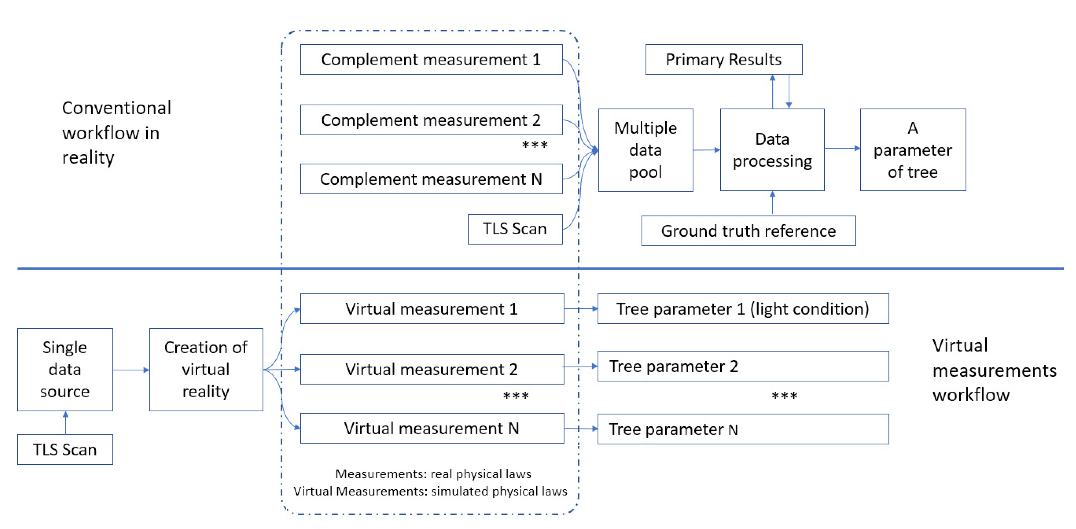
2.1.2. Mechanism of VMW

According to the mission of VMW, we determined the mechanism of VMW. The key to VMW was to apply virtual measurements in virtual spaces instead of forest measurements in reality. Consequently, the measuring target changed from real trees to the corresponding virtual trees. Therefore, the necessary complementary measurements would have the same timestamp in the original point cloud. VMW had three components, i.e., archived data source, virtual trees, and virtual measurement. The archived data sources were the only data source. The use of VMW for a specific tree parameter was called the implementation of VMW.

2.1.3. Virtual Trees, the Equivalents of Real Trees

The change of the measuring target from real trees to virtual trees was the basis of VMW. Ideally, each virtual tree was exactly equal to the corresponding real tree. The format of virtual trees could vary due to different tasks. The primary level of virtual trees was the original point cloud of trees. This level of virtual trees preserved all information stored in the original point cloud. It was recommended to be used as the measuring target for virtual measurement. However, the compositional form of these virtual trees, i.e., x, y, z, and intensity, was far away from the natural structure of trees. For this reason, tree models derived from the original point cloud were recommended as virtual trees at secondary levels. Compared to the primary level, loss of information was unavoidable due to the introduction of additional data processing, i.e., modeling.
Modeling was a process of converting a point cloud into a virtual tree at secondary levels. Current modeling methods usually model trees by using cylinders or voxels [36,37]. Each of them granted tree models a solid entity with volume that was close to the natural structure of the trees. There were two side effects that accompanied the modeling process: (a) missing information and (b) adding false information. Effect (a) was acceptable and effect (b) required to be avoided. After establishing the geometric properties of virtual trees, physical properties were added. In the final step, virtual trees could respond to external detection in virtual reality.

2.1.4. Computational Virtual Measurement, the Equivalents of Measurement in Reality

In reality, trees were observed by measurement instruments by using basic physical laws. Correspondingly, we developed computational virtual measurement (CVM) to measure virtual trees using simulated physical laws in virtual reality. The purpose of the design of CVM was to have the same timestamp in the original point cloud. Meanwhile, it was expected to bypass the need for validation and calibration of results due to the lack of reference data. By learning from real measurement process, the measurement result was determined using purely physical processes and did not require mathematical predictions. According to this feature, CVM was designed as a virtual physical process that aimed to measure virtual trees using virtual measurement instrument (VMI), which is similar to how real trees are measured in nature. VMI was the set name of all physical processes that are simulated in virtual spaces. The accuracy of a CVM process depends on the accuracy of the simulation of the basic physical laws. Those simulations could be provided by third-party applications such as PhysX and Unity with ultra-high precision [38,39]. The process was not in the same order of magnitude as the accuracy of TLS scanning or tree modeling. Therefore, we did not consider it necessary to calibrate the basic physical laws.

2.2. An Example of How to Implement VMW: Virtual Measurement of Light Conditions

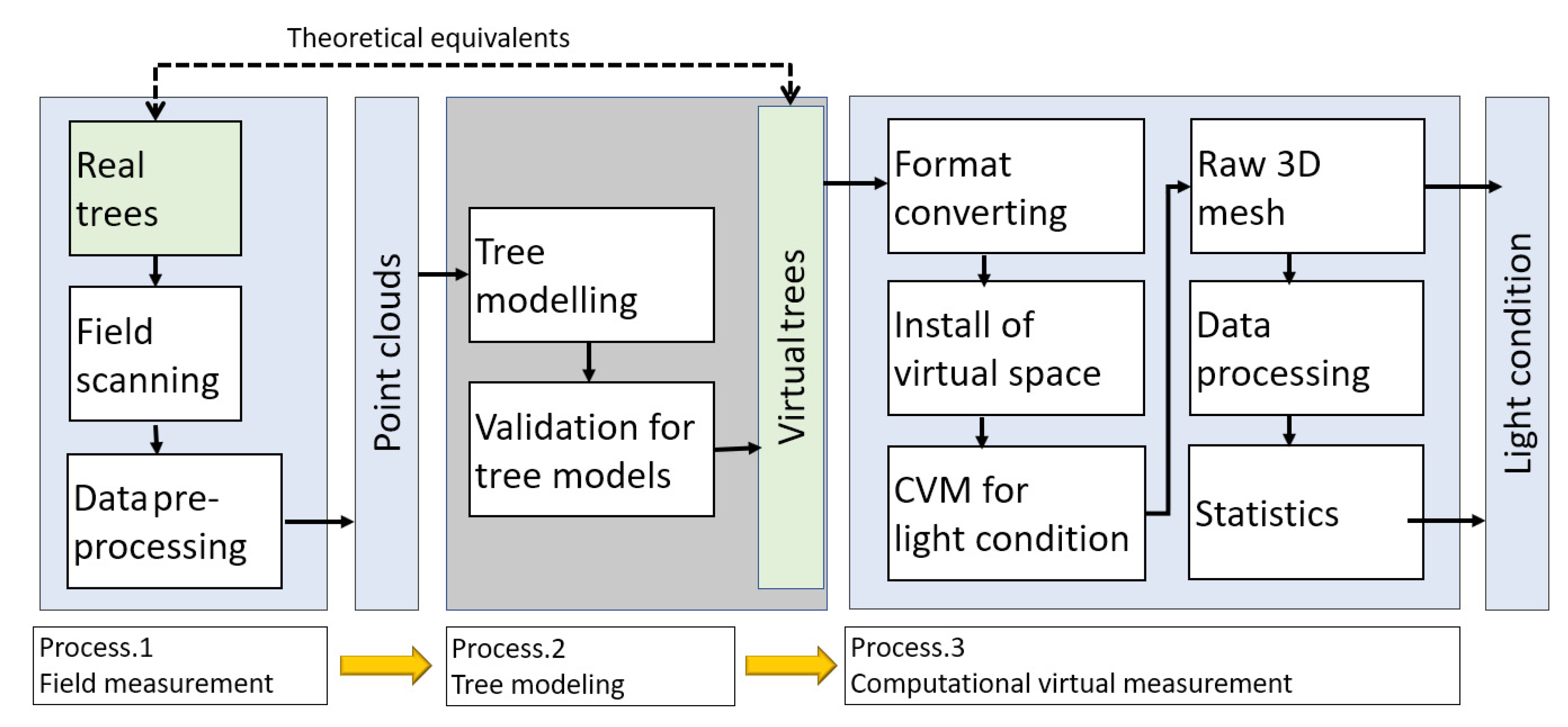
2.2.1. Full Workflow

According to the method description of VMW, Figure 2 shows the detailed workflow starting from the real trees (in the original sample plot) to the data mining result of light conditions. In process.2, we employed quantitative structure model (QSM) methods to construct virtual trees [40]. QSM models were facile to edit tree models manually for validation and calibration than compared to voxel modeling methods [36]. In process.3, SketchUp (Trimble, California, USA) was used to provide a virtual 3D Euclidean space [41]. After that, the simulation of radiation sensor (recording the lights on/off) and the sunlight illumination was executed by Sunshine_pro_2019 (Arcdot, Beijing, China). In the final step, we conducted statistics based on the analysis results.

2.2.2. An Archived Point Clouds from TLS Field Campaign

One of the problems with data mining was that we were not able to participate in the original TLS scan. As a result, the data quality of the archived point cloud may negatively affect the data processing. Similar to the point cloud used in this study and compared to a typical setting for the single tree scanning [42], there was an absence of a scan position in the west-south area in this TLS scan. This absence of scan position was common in field measurements. Many factors, such as tree density, season, accessibility, and terrain, prevent an ideal distribution of scanning positions for single tree modeling. This problem was considered as a major challenge for the reuse of point clouds. Indeed, we could employ algorithms that utilize massive predictions to generate fine models [43]. Accordingly, tree models with massive predictions would depart from the definition of the virtual tree. However, from this set of data, we acknowledged that data faults were common in archived data. As of yet, we are unaware of how to establish a standard for accepting virtual trees that includes predictive components. Currently, this condition is generally prohibited. This is something that deserved further discussion.
On 14 January 2015 (winter season, leaf-off), the field data collection was carried out on the campus of Beijing Forestry University (40°0′07″ N; 116°20′33″ E). The original purpose of this campaign was to generally scan campus buildings from multiple scan positions. The TLS scanner used was FARO Photon 120 scanner (FARO Technologies Inc., Orlando, FL, USA). The scan mode was set to 360° horizontal scanning. The scan speed was set to 244,000 pts/sec. No reflectors or reference balls were implanted during the scan. Table 2 shows the specifications of the TLS scanner.
The tree species was the American sycamore (Platanus occidentalis L.) and the trees have been planted as landscape trees. This area was approximately 15 m × 25 m in size and surrounded by three scan positions. By visual inspection of point clouds from all scan position, we found an area containing eight trees that had the potential to be made as fine tree models. However, only one tree met the criteria of virtual trees. Other trees were excluded.

2.2.3. Data Pre-Processing

The purpose of the data pre-processing was to extract point clouds for single trees from the raw TLS scans. We used the registration tools in CloudCompare (EDF, Paris, France) [44] by point pair picking to register point clouds from different scans. The point pairs were chosen at the corners of the campus building. After that, a rough dataset for the single tree was segmented manually.
Denoising and leaf removal were critical works in data pre-processing. Based on the rough segmentation of the point cloud, we utilized manual deletion for the apparent parts, which did not belong to the single tree. Then, a voxel-based outlier filter was applied to remove the discrete points [45]. All the remaining points were clustered spatially using the density-based spatial clustering of applications with the noise (DBSCAN) method [46]. Different thresholds were tested and the results were inspected visually.
The process of leaf removal was similar to denoising works. The leaves were regarded as noises in this study. A curvature filtering was applied to the point cloud. This method was based on principal components analysis (PCA) for point’s neighborhood [47]. Appropriate PCA parameters could distinguish the leaf from the stem structure of the tree. In the end, we added a manual deletion for the remaining leaves and manually repaired some points on the stem that were incorrectly deleted by algorithms.

2.2.4. Tree Modeling and Validation

The role of the tree model is to provide a radiation receiver to receive virtual sunlight in virtual spaces. We applied the QSM method to model the tree using SimpleTree (Jan Hackenberg, Freiburg, Germany) [47]. This application was also utilized in data pre-processing. SimpleTree is a user-friendly software and responded instantly to the change of parameters. Several parameters affected the tree modeling process. Initially, we applied the default settings in SimpleTree with the function of parameter optimization [47]. The outputted model was evaluated using visual inspection by overlaying the model with the point cloud. Furthermore, we applied tiny random changes with the amplitude within 5% on the modeling parameters to find better modeling results.
No external reference was required for the validation of the tree model. We preferred to use the visual inspection. This is because the original point cloud itself was the ground truth reference for the spatial distribution of the tree structure. Many studies used the comparison of physical quantities, e.g., stem volume, to validate tree models [36,42,47,48]. However, from our perspective, the simple quantitative consistency had no relationship to the correct distribution of tree structure. Therefore, overlaying was an effective method. During the visual inspection, manual corrections were made to tree models. Finally, the corrected tree model was regarded as virtual trees for subsequent CVM processing.

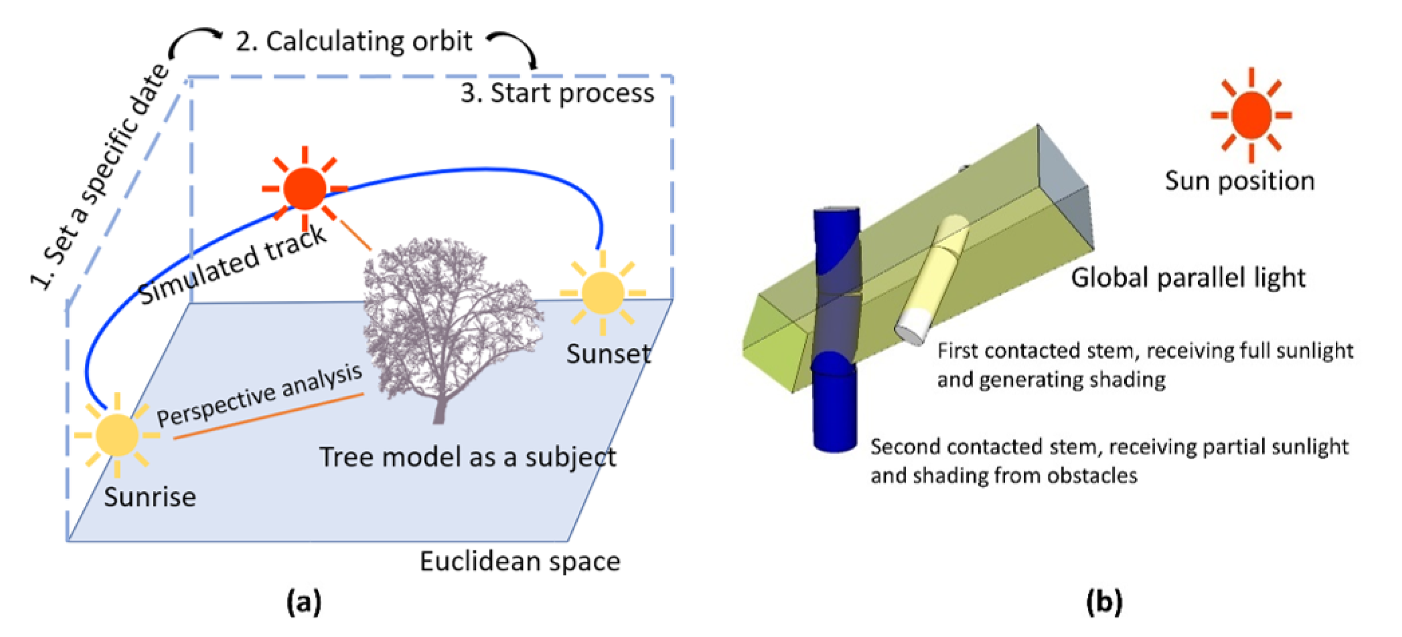
2.2.5. CVM for Single Tree Light Conditions

Light condition measurement is the central process in this study. Compared to instant methods in Table 1, light condition measurement is a dynamic method that measures the virtual tree from sunrise to sunset. Moreover, it is a direct and full sampling measuring method that removes the need of validation, calibration, and systematic sampling procedure. Previous steps prepared the virtual space and the virtual tree as a static radiation receiver. In this step, the motion of the sun in the sky, the sunlight emission, the shading in the tree structure, and the virtual radiation receiver were simulated by Sunshine_pro_2019. Those four simulations contributed together as a specific virtual measuring tool for light condition measurement.
Figure 3a describes the full process of light condition measurement during the daytime. The virtual measurement started at the point of sunrise. According to a user-defined period, the position of the virtual sun changed step by step. In each step, a vector was calculated using the position of the virtual sun and the tree model to determine the direction of virtual sunlight. Then, a global parallel light was generated to illustrate entire rooms in the virtual space and followed with prospective analysis [48]. Figure 3b shows the detailed demonstration of perspective analysis.
Sunshine_pro_2019, which is a plugin in SketchUp, was applied to perform light condition measurement in this study. It is an application for assessing light conditions for buildings [49]. We analyzed the similarity between tree models and building models. Both of them have multiple faces and vertexes. They spread their bodies in 3D Euclidean space with exclusive occupation. Therefore, we tested Sunshine_pro_2019 and successfully processed the demo tree model for assessing light conditions. Moreover, the process for the demo tree model was restricted by the free licensed version. The simulation of sun motion was fixed in 6 and 8 h on two specific days.
The parameters applied in the Sunshine_pro_2019 are as follows: (geolocation: 40°0′07″ N, 116°20′33″ E; date: “Da Han Ri”, which refers to 20 January, sunrise at 07:33:08, and sunset at 17:18:56, simulating time span: 08:00:00 to 16:00:00; sweep angle: not set; minimal sunshine duration: 5 min; sample point spacing: 0.5 m; time interval of sun position: 8 min). Notably, we magnified the tree model 30 times for each side length. Consequently, the equivalent sample point spacing for the original tree model is 1.67 cm.

2.2.6. Technical Issues of Using Architectural Software

In this study, virtual reality and virtual measurements were performed using architectural software. Daylight assessment is a standardized process that has to be involved in the design of buildings. Accordingly, the relevant algorithms have been developed for decades and reached a steady-state. We utilized the credibility of its calculation and replaced buildings with trees. It was also our attempt to find utilization of architectural software on forest science. Due to the different scale between buildings and trees, there were some technical issues that needed to be addressed.
One should be cautious when scaling the original tree model since the smallest input for sample point spacing in Sunshine_pro_2019 is 0.5 m. Therefore, we magnified the tree model 30 times on each side length. Consequently, the smallest equivalent sample point spacing for the original tree model was 1.67 cm. In the case of a blank value, it is necessary to perform a visual inspection of the result. The acceptable requirement is that all visible parts of the tree model were granted a color attribute. In addition to visual inspections, directly checking the plain text in the resulting 3D mesh is another method to make validations. Moreover, the independent 2D flat should not exist in the tree model because Sunshine_pro_2019 was designed to analyze the 3D building. A 2D flat might cause duplicate rendering.

2.2.7. Data Format of the Output

The output was the duration of sunlight exposure in relation to the surface area on the stem. This output was attached to the surface of the tree model (virtual tree). Prior to the CVM process, surfaces of the tree model were all indistinguishable from one another without the parameter of exposure duration of direct irradiation. After completing the CVM process, each surface would be granted exposure duration. If an original surface had a different exposure duration, it would be divided into different and smaller new surfaces.

2.2.8. Statistics

The result for light condition measurement is a 3D mesh using the format of the wavefront (obj), which is a commonly used 3D format in computer graphics [46]. Obj files use plain text to record 3D geometry including the following elements: vertex coordinates, vertex normals, faces with their corresponding vertices, texture vertices, texture rendering, and UV position for texture filling. We took vertex coordinates, faces with their corresponding vertices, and texture rendering from the outputted mesh as the new processing dataset. In this processing dataset, we calculated the area of each triangle [50] and read the information of color and height. Four elements, i.e., the processing order, the area of the triangle, the color, and the height, culminated together to form the final result dataset. Finally, the final result dataset was imported into MATLAB for further statistical analysis. Furthermore, the obj file is also the middleware for transferring data between different applications.
The statistical output of light condition measurement contains the information of area connected with exposure duration with nine groups that consists of 0–1 h, 1–2 h, 2–3 h, 3–4 h, 4–5 h, 5–6 h, 6–7 h, and 8 h. Furthermore, additional information is provided: (i) The relative area of faces (triangles) is the area of all faces in an exposure duration group divided by the full surface area of the stem; (ii) the relative quantities of faces (triangles) is the quantity of all faces in an exposure duration group divided by the overall quantity of faces in the 3D result model; (iii) a ratio is the relative area of faces (triangles) divided by relative quantities of faces (triangles).

2.2.9. Additional Data Source

An additional data source was employed to test the versatility and robustness of the VMW implementation of light condition measurements. This data source was provided by simpleforest.org and included point clouds of four common types of trees. Each tree in this dataset was exactly processed using the same procedure presented in Section 2.2.1, Section 2.2.2, Section 2.2.3, Section 2.2.4, Section 2.2.5, Section 2.2.6, Section 2.2.7 and Section 2.2.8. In addition to the test of generality and robustness, it also contributed to analysis on tree morphology and physiology.

3. Results

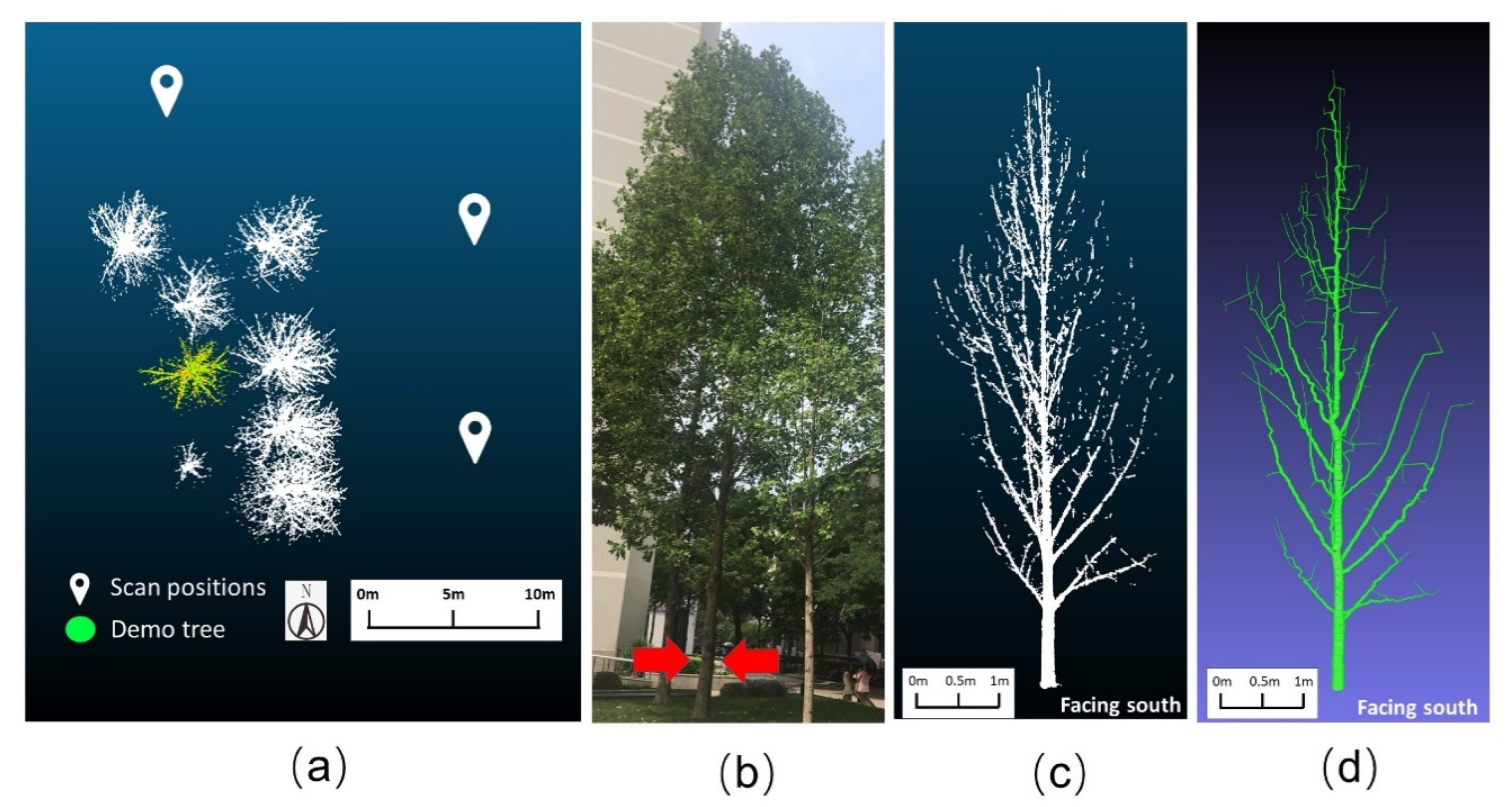
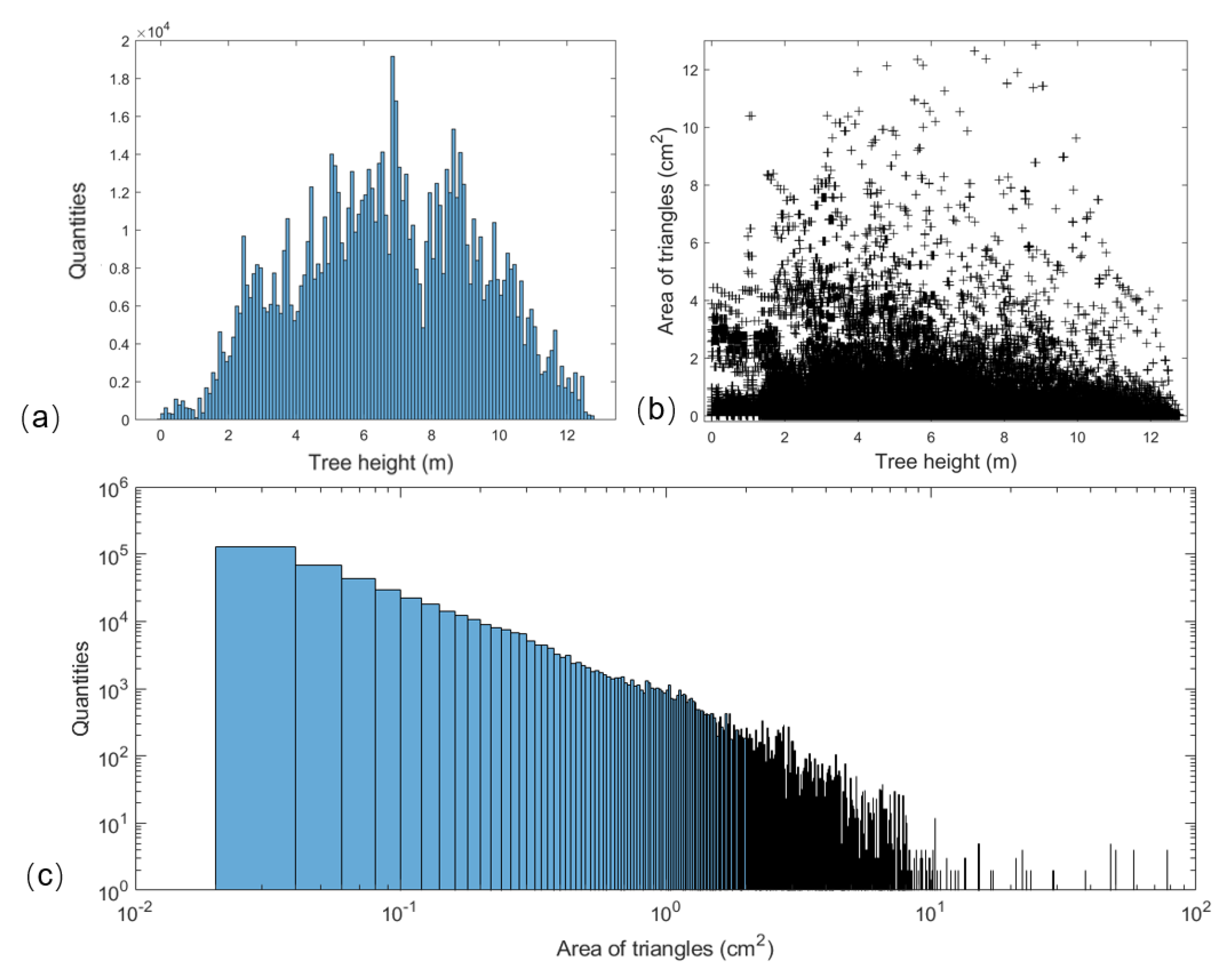
3.1. TLS Scanning and Single Tree Modeling

The TLS scanning and QSM modeling results are shown in Figure 4. The impact on data quality concentrated on the QSM modeling process. As shown in Figure 4a, there are a green tree and seven white trees in the sample plot. The original plan was to apply QSM modeling in all the eight trees. However, due to the obstacles and the lack of one scanning position, only one tree (the green tree) was successfully modeled. Figure 4b is a photo of the green tree. Figure 4c showed the point cloud after data pre-processing. Figure 4d showed the QSM model after manual correction.
The measured tree parameters are as follows: the tree height is 12.81 m; the DBH is 24.60 cm; the stem volume from the QSM model is 0.52 m3. It is noticeable that we manually modified the obvious modeling error on the main stem part by using another 3D modeling tool, Blender [51]. Thus, the stem volume of the tree model, shown in Figure 4d, has a minor difference with the original QSM model. The area of stem surface was re-calculated using the method stated in Section 2.2.8.

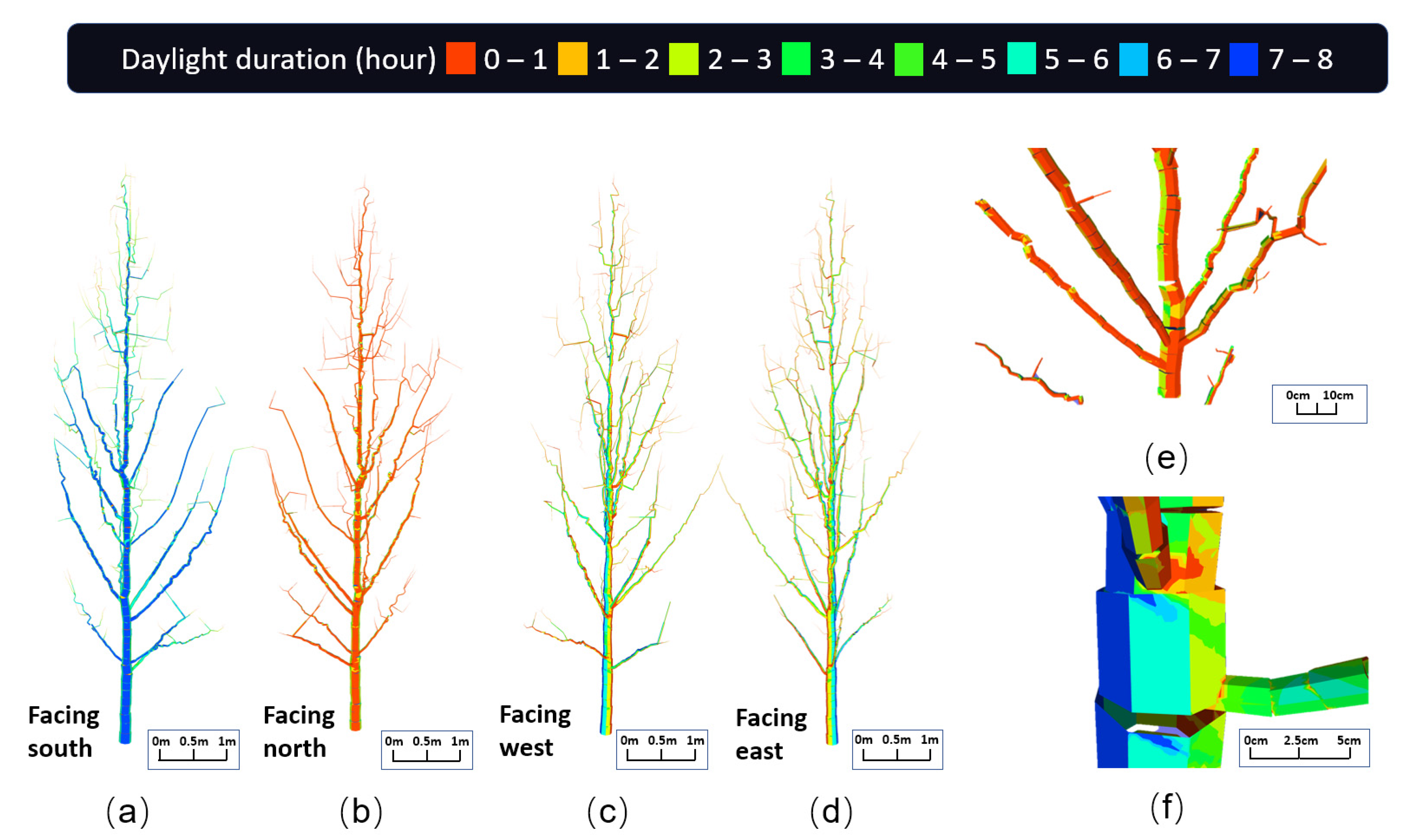
3.2. CVM for Single Tree Light Condtions

The results of light condition measurement on the demo tree model are shown in Figure 5. The result was outputted as a 3D mesh with an additional attribute, i.e., the color. Eight different colors are used to represent different daylight durations on the corresponding parts of the tree. The original tree model had 31,706 faces (organized using triangles). For an original face, e.g., the generally cyan-blue face in Figure 5f, it would have different exposure durations to the direct illustrated sunlight. Therefore, each original face would be divided into a few new faces, unless it could not receive virtual sunlight during the entire simulation (facing north). Specifically, for the demo tree in this study, the number of faces (triangles) increased from 31,706 to 899,346 after light condition measurement. Figure 5a–d are the views of the result from different directions. Figure 5e,f are partially magnified views of the result on different scales.
Sunshine_pro_2019 could not provide any statistical information. It only stored the exposed duration information as the color attribute in the obj file. According to the method stated in Section 2.2.8, we developed an application using C# to read the information directly in the obj file. Then, the information was imported into MATLAB for further statistical procedures. Figure 6 shows the statistical result of the light condition measurement for the whole tree model.
Figure 7 shows the distribution of the area of faces (triangles) in tree height classified by sunlight duration. Most importantly, Figure 7i shows that the locations of triangles concentrating in the lower position on the tree compared to other daylight groups (a–h). The relatively large percentage of large triangles in Figure 7i also indicates that those triangles are on the surface of the main stems.
Table 3 is the final result we obtained from this study. It shows the temporal and spatial distribution of solar energy (via direct irradiation) on a single tree in general. Compared to the 3D result mesh, detailed information on a specific face is lost. To sum up, light condition measurement provides the result with two forms. The first one is the 3D result mesh, which contains full information. The second one are the statistical results from the 3D result mesh, which are appropriate for citation in papers.
Table 3 shows that there was only 4.34% of the tree structure exposed in the sunlight during the 8 h of the study simulation. The amount of 35.87% of the tree structures was covered with sunlight in less than one hour. We made the assumption to apply a light condition measurement on a regularly shaped object, e.g., a cube, which has five square faces (excluding the bottom) and one face is directed to geographical (true) north. For this cube, the sunlight duration of less than one hour would be precisely at 20%, which significantly differed to 35.87%. This difference indicates that the shadings between tree structures have a significant influence on the duration of daylight (direct illumination).

4. Discussion

4.1. Discussion for VMW

4.1.1. Choices of Modeling Levels of Virtual Trees

An ideal tree model records the tree structures at 100 percent. Theoretically, each part of the tree model should have a corresponding element in the real tree. However, all the current tree models are the subsets of this ideal tree model. Therefore, the tree models, which approach the ideal tree model, should be the priority. Under this consideration, the tree models with leaves seemed to be the best choice. However, there were no effective methods to validate the leaves generated by algorithms. That is to say that the validation processes prevented the utilization of leaf models. Some complicated methods could record the positional structure of each leaf in a tree and the predicted leaf could not correspond to a pair on the real tree. Therefore, validation at the leaf level seems to be impossible.
As previously stated in Section 1.1 and Section 1.2, the NFI sample plot measurements are not aimed at the validating site-specific or tree-specific methods. More specifically, only the raw point cloud contains positional ground true information for tree structures. The process is to overlap the tree model with the raw point cloud. Previous studies showed that virtual human inspection is the only method to evaluate the accuracy of tree models on spatial distribution [40,42,52]. However, these methods of comparison between tree model-derived parameters and reference data of overall trees are not helpful in evaluating the spatial distributions of tree parts.
According to the concept of CVM, the tree model is only used as a representative of the corresponding real tree at this moment. Therefore, the criteria of how to choose the levels of tree model should be considered from two aspects. The primary aspect is that the tree model should be validated without any additional data sources. The additional methods in sample plots may increase the workload in each sample plot nationwide. The secondary aspect is that the tree model is more precise at higher modeling levels. Under these criteria, three tree modeling levels should be tested, i.e., at the stem level, at the crown level, and at the leaf level. However, the tree model with the leaf was excluded due to the lack of validation methods. The tree model with the crown was excluded due to the fact that the outliners of the tree crown concealed the inner structure of canopies. In the end, the tree stem model was utilized because it could be validated with the raw point cloud.

4.1.2. A Theoretical Preparation for Lidar-Based NFI in the Future

VMW was developed originally for data mining and data utilization. During the demonstration implementation of VMW, it was found that it had the potential to contribute to an assumed LiDAR-based NFI in the future. Lidar-based NFI was our vision for the next generation of NFI. This vision was based on the assumption that the hardware limitations of TLS could be eliminated. In this condition, we could get an instantaneous snapshot of a sample plot without loss of information.
The first change would happen in the field measurements. Currently, multiple instruments and human perceptions were employed together that complicated the sources of error. If TLS was used, all measurement targets in the sample plots would have the same measurement process. It facilitated the standardization of the measurement process and the control of data quality. The second change would be in the form of raw data. From the perspective of data preservations and data utilization, the Text was weak and fragile. In comparison, point clouds would have a huge advantage in the following aspects: (a) It is more subject than limited tree parameters in the log sheet; (b) it has rich information compared to the few tree parameters in Text; (c) maintainability of data and (d) expandability using data mining.
Based on point clouds, virtual sample plots could be formulated. By applying VMW, tree parameters would be extracted from virtual sample plots. Compared to being directly logged using Text, it would have the chance to review, maintain, and upgrade. Furthermore, new methods developed in the future could be directly applied to the virtual sample plot, such as the implementation of VMW for assessing light conditions of single trees in this study. It demonstrated in detail how to use VMW for specific purposes. Thus, this is how an archived NFI sample plot could stay up to date.

4.2. Discussion for VMW Implementation of Light Condiction Measurement

The VMW implementation of light condition measurement served as an example of how VMW could be implemented for a specific tree parameter. It provided raw measurement data and temporal and spatial distribution of solar energy on the stem (bark) surface, which was not an intended conclusion for a specific study topic. In this section, we presented several demonstrations on how to utilize this kind of data for further studies.

4.2.1. Investigation of the Connection between Light Conditions and Tree Morphology

The exposed duration for tree surfaces depends both on the surface orientation and shades from obstacles. The effect of orientation and shades can be quantitatively determined by light condition measurement. For the demo tree, the percentage of full lighting in the tree surfaces was virtually measured to be 4.34% (marked “α” in Table 2). The distributions of the area of faces (triangles) in tree height are classified by sunlight duration in Figure 7. The faces of full exposure are recorded in Figure 7i. The data distribution is significantly different from the other graphs in Figure 7. Those faces in Figure 7i are concentrated in the lower height of the tree with a large face area. Considering the images in Figure 5a–d, we noticed that the lower height of the tree model referred to the main stem with a few branches. For the first time, two small branches are in at a height of around 1.6 m. Then, three main branches are at a height of about 2.8 m. When increasing by height, more branches appeared in the tree model, which projects shades relative to other tree structures. Thus, an original face in the upper height of the tree is most likely to be split into smaller faces (shown in Figure 5f). There is little chance for large area faces of full exposure in the upper height of tree and little chance for a continuous distribution of faces with the same exposure duration.
We calculated the ratio between the relative area of faces and relative quantities of faces to be “The ratio of α/β” in Table 3. The representative ratio of α/β, i.e., γ (marked “γ” in Table 2), indicates this ratio in the group of 8 h exposure. The smaller the value of γ, the more significant the dispersion degrees for faces (triangles) in the spatial distribution. Compared to other ratios in different time groups, the high value in γ indicates that the average area for faces in this time group was larger than the others. Regarding the graphs in Figure 7i and Figure 4, γ demonstrated that these faces with large areas are more likely distributed on lower stems. The α and γ values might associate with the phototaxis of tree organism growth affecting the overall tree skeleton structures. For each individual branch in the tree, obtaining more solar energy was essential for the development of the foliage clump attached to the branch. Only the lower stem could be exposed to the sunlight continuously, which makes the trunks bathe in sunlight with the enhanced capability to resist diseases and pests and strengthen the wooden material to provide mechanical stability for the upper tree crown.
In addition to the investigation of single trees, VMW implementation of light condition measurements could also be considered as a tool for analyzing the morphology of trees among different tree species. Four virtual trees of four tree species were measured. Each part of the virtual trees was granted the daylight duration in different colors in Figure 8. Table 4 shows the daylight duration classified by hours.
We tried to investigate the differences in sunlight absorption by these four species of trees. In Table 4, more than 10% of the surface on the gemu tree was illuminated throughout the day (8 h), which was the highest among the four trees. It indicates that the crown structure of the gemu tree was the simplest of cylindrical tree crown with a narrow tree skeleton, as shown in Figure 8b. If a tree could only receive light for a short period of time on most of its surface, its crown may then have a complex internal structure. High-frequency shading could prevent continuous irradiation of a single spot on tree skeleton. For example, the cherry tree (Figure 8d) has the case shape of the tree crown and with serious self-occluded region existence. In Figure 8b,c, the gemu tree and the Masson’s pines had similar height and DBH. The difference between them was the shape of the crown, i.e., dispersed and elliptical tree crown shapes, respectively. The output of VMW implementation of light conditions had good differentiation for different crown structures. Therefore, it might continue to develop as a tool for identifying the effects of various crown shapes on radiosity for different tree species.

4.2.2. Potential Contributions to Tree Physiology Research

In addition to tree morphology, this VMW implementation may further contribute to research in tree physiology studies. For instance, non-photosynthetic activities driven by sunlight were also of vital importance for the physiological activities of trees [53]. In contrast to photosynthetic activities, photoreceptors for non-photosynthetic activities were diverse and distributed in different organs of the plant, affecting the growth of stems [52]. In order to investigate non-photosynthetic activities quantitatively, it is usual to apply experiments under laboratory conditions [54,55]. Such experimental conditions were hard to apply in the sample plot in forests. The output of VMW implementation of light condition measurement was expected to provide supporting data for those studies for trees in forests.
For some particular tree species, e.g., the coconut palm (Cocos nucifera) and European black elder (Sambucus nigra L.), understanding the distribution of sunlight on the stem was significant to investigating the development of timber volume. This was because the stems of those trees had particular biological structures or functions, which were always exposed to sunlight. For example, coconut palm did not possess bark. Instead, the epidermis hardened and formed protective layers [56]. Considering that the common habitat of the coconut palm [57], environmental factors, including solar exposure, would be the factors to investigate the aging process of trees [58]. Another example was the European black elder, which possessed a chlorophyll layer under the bark [59]. The output of VMW implementation of light condition measurement was expected to contribute to the calculation of solar energy conversion rate.
Sunlight-driven activities in the exterior of trees also impacted the growth of trees. For example, the relationship between direct sunlight and insect activity was recognized in the early times [60]. We foresaw that the output (the 3D mesh) could provide useful raw data accompanying other factors [61] and it could produce maps of the possibilities of insects (driven by lights) landing and inhabiting stems and bark. Another example was that sunlight exposure was an indicator of forest fire [62]. By applying this VMW implementation in a forest sample site on multiple trees, it could help to identify areas with high concentrations of solar energy in the leaf-off seasons.

5. Conclusions

The overall purpose of this study was to call attention to the value of archived TLS data, which contains rich unexploited information and could further benefit related studies. In order to overcome the inconsistency of timestamps, we successfully developed VMW in this study. The basic mechanism of VMW was to apply virtual measurement instead of real measurements in the forest field. With the exception of being a practical data mining tool for archived lidar point clouds, the feasibility of VMW was demonstrated and proved by assessing the light condition of single tree using VMW. The output of this implementation was raw measuring data such as tree height and DBH. We further demonstrated how to use this type of data with several examples in tree morphology and physiology. In addition to data mining, VMW had shown potential as a standardized data processing tool. We foresee that virtual measurements on virtual trees and virtual sample plots would also be a hot research topic in the near future.

Author Contributions

Conceptualization, Z.W.; data curation, J.Z. and J.W.; formal analysis, Z.W.; investigation, J.W. and Y.Z.; methodology, Z.W. and X.Z.; resources, J.W.; software, Z.W. and X.Z.; supervision, C.S.; visualization, Z.W.; writing—original draft, Z.W.; writing—review and editing, Z.W. and C.S. All authors have read and agreed to the published version of the manuscript.

Funding

This research was funded by the China Scholarship Council (CSC); the project number is 201306510005.

Institutional Review Board Statement

Not applicable.

Informed Consent Statement

Not applicable.

Data Availability Statement

The single tree in the Section 2.2.2 can be download from https://static.hikstorage.com:8080/share/index.html?shareId=c18cceedbeed53361ef744983defc2ba, using password: 4029, accessed on 18 June 2021. Dataset (from the 3rd party) in the Section 2.2.9 can be download from simpleforest.org, accessed on 18 June 2021. Any other data is available on request from [email protected] by email.

Acknowledgments

We thank the China Scholarship Council (CSC) for research funding.

Conflicts of Interest

The authors declare no conflict of interest.

References

  1. Liang, X.; Hyyppä, J.; Kaartinen, H.; Lehtomäki, M.; Pyörälä, J.; Pfeifer, N.; Holopainen, M.; Brolly, G.; Francesco, P.; Hackenberg, J.; et al. International benchmarking of terrestrial laser scanning approaches for forest inventories. ISPRS J. Photogramm. Remote Sens. 2018, 144, 137–179. [Google Scholar] [CrossRef]
  2. Liang, X.L.; Kankare, V.; Hyyppa, J.; Wang, Y.S.; Kukko, A.; Haggren, H.; Yu, X.W.; Kaartinen, H.; Jaakkola, A.; Guan, F.Y.; et al. Terrestrial laser scanning in forest inventories. ISPRS J. Photogramm. Remote Sens. 2016, 115, 63–77. [Google Scholar] [CrossRef]
  3. Kulman, H. Effects of insect defoliation on growth and mortality of trees. Annu. Rev. Entomol. 1971, 16, 289–324. [Google Scholar] [CrossRef]
  4. Li, Y.; Härdtle, W.; Bruelheide, H.; Nadrowski, K.; Scholten, T.; von Wehrden, H.; von Oheimb, G. Site and neighborhood effects on growth of tree saplings in subtropical plantations (China). For. Ecol. Manag. 2014, 327, 118–127. [Google Scholar] [CrossRef]
  5. Latifi, H.; Fassnacht, F.E.; Müller, J.; Tharani, A.; Dech, S.; Heurich, M. Forest inventories by lidar data: A comparison of single tree segmentation and metric-based methods for inventories of a heterogeneous temperate forest. Int. J. Appl. Earth Obs. 2015, 42, 162–174. [Google Scholar] [CrossRef]
  6. Magnussen, S.; Naesset, E.; Gobakken, T. Lidar-supported estimation of change in forest biomass with time-invariant regression models. Can. J. For. Res. 2015, 45, 1514–1523. [Google Scholar] [CrossRef]
  7. Stovall, A.E.L.; Vorster, A.G.; Anderson, R.S.; Evangelista, P.H.; Shugart, H.H. Non-destructive aboveground biomass estimation of coniferous trees using terrestrial lidar. Remote Sens. Environ. 2017, 200, 31–42. [Google Scholar] [CrossRef]
  8. Oberbauer, S.F.; Strain, B.R. Photosynthesis and successional status of costa rican rain forest trees. Photosynth. Res. 1984, 5, 227–232. [Google Scholar] [CrossRef]
  9. Green, S.R. Radiation balance, transpiration and photosynthesis of an isolated tree. Agric. For. Meteorol. 1993, 64, 201–221. [Google Scholar] [CrossRef]
  10. Iwasa, Y.; Cohen, D.; Leon, J.A. Tree height and crown shape, as results of competitive games. J. Theor. Biol. 1985, 112, 279–297. [Google Scholar] [CrossRef]
  11. Kozlowski, T.T. Light and water in relation to growth and competition of piedmont forest tree species. Ecol. Monogr. 1949, 19, 207–231. [Google Scholar] [CrossRef]
  12. Gravel, D.; Canham, C.D.; Beaudet, M.; Messier, C. Shade tolerance, canopy gaps and mechanisms of coexistence of forest trees. Oikos 2010, 119, 475–484. [Google Scholar] [CrossRef] [Green Version]
  13. Gendron, F.; Messier, C.; Comeau, P.G. Comparison of various methods for estimating the mean growing season percent photosynthetic photon flux density in forests. Agric. For. Meteorol. 1998, 92, 55–70. [Google Scholar] [CrossRef] [Green Version]
  14. Kato, S.; Komiyama, A. Spatial and seasonal heterogeneity in understory light conditions caused by differential leaf flushing of deciduous overstory trees. Ecol. Res. 2002, 17, 687–693. [Google Scholar] [CrossRef]
  15. Parent, S.; Messier, C. A simple and efficient method to estimate microsite light availability under a forest canopy. Can. J. For. Res. 1996, 26, 151–154. [Google Scholar] [CrossRef]
  16. Bunce, J.A. Effects of weather during leaf development on photosynthetic characteristics of soybean leaves. Photosynth. Res. 1985, 6, 215–220. [Google Scholar] [CrossRef]
  17. Pretzsch, H. Canopy space filling and tree crown morphology in mixed-species stands compared with monocultures. For. Ecol. Manag. 2014, 327, 251–264. [Google Scholar] [CrossRef] [Green Version]
  18. Deleuze, C.; Hervé, J.-C.; Colin, F.; Ribeyrolles, L. Modelling crown shape of piceaabies: Spacing effects. Can. J. For. Res. 1996, 26, 1957–1966. [Google Scholar] [CrossRef]
  19. Pretzsch, H. Re-evaluation of allometry: State-of-the-art and perspective regarding individuals and stands of woody plants. In Progress in Botany 71; Springer: Berlin/Heidelberg, Germany, 2010; pp. 339–369. [Google Scholar]
  20. Peper, P.J.; McPherson, E.G.; Mori, S.M. Equations for predicting diameter, height, crown width, and leaf area of san joaquin valley street trees. J. Arboric. 2001, 27, 306–317. [Google Scholar]
  21. Bechtold, W.A. Largest-crown-width prediction models for 53 species in the western united states. West. J. Appl. For. 2004, 19, 245–251. [Google Scholar] [CrossRef]
  22. Ferraz, A.; Saatchi, S.; Mallet, C.; Meyer, V. Lidar detection of individual tree size in tropical forests. Remote Sens. Environ. 2016, 183, 318–333. [Google Scholar] [CrossRef]
  23. Whitmore, T. Canopy gaps and the two major groups of forest trees. Ecology 1989, 70, 536–538. [Google Scholar] [CrossRef]
  24. Bagaram, M.; Giuliarelli, D.; Chirici, G.; Giannetti, F.; Barbati, A. Uav remote sensing for biodiversity monitoring: Are forest canopy gaps good covariates? Remote Sens. 2018, 10, 1397. [Google Scholar]
  25. Yun, T.; Jiang, K.; Li, G.; Eichhorn, M.P.; Fan, J.; Liu, F.; Chen, B.; An, F.; Cao, L. Individual tree crown segmentation from airborne lidar data using a novel gaussian filter and energy function minimization-based approach. Remote Sens. Environ. 2021, 256, 112307. [Google Scholar] [CrossRef]
  26. Yun, T.; Cao, L.; An, F.; Chen, B.; Xue, L.; Li, W.; Pincebourde, S.; Smith, M.J.; Eichhorn, M.P. Simulation of multi-platform lidar for assessing total leaf area in tree crowns. Agric. For. Meteorol. 2019, 276, 107610. [Google Scholar] [CrossRef]
  27. Bréda, N.J. Ground-based measurements of leaf area index: A review of methods, instruments and current controversies. J. Exp. Bot. 2003, 54, 2403–2417. [Google Scholar] [CrossRef]
  28. Weiss, M.; Baret, F.; Smith, G.; Jonckheere, I.; Coppin, P. Review of methods for in situ leaf area index (lai) determination: Part ii. Estimation of lai, errors and sampling. Agric. For. Meteorol. 2004, 121, 37–53. [Google Scholar] [CrossRef]
  29. Kitao, M.; Hida, T.; Eguchi, N.; Tobita, H.; Utsugi, H.; Uemura, A.; Kitaoka, S.; Koike, T. Light compensation points in shade-grown seedlings of deciduous broadleaf tree species with different successional traits raised under elevated co2. Plant Biol. 2016, 18, 22–27. [Google Scholar] [CrossRef] [Green Version]
  30. Song, Q.; Xiao, H.; Xiao, X.; Zhu, X.-G. A new canopy photosynthesis and transpiration measurement system (capts) for canopy gas exchange research. Agric. For. Meteorol. 2016, 217, 101–107. [Google Scholar] [CrossRef]
  31. Hu, Y.; Zhao, P.; Niu, J.; Sun, Z.; Zhu, L.; Ni, G. Canopy stomatal uptake of nox, so2 and o3 by mature urban plantations based on sap flow measurement. Atmos. Environ. 2016, 125, 165–177. [Google Scholar] [CrossRef]
  32. Jaakkola, A.; Hyyppä, J.; Yu, X.; Kukko, A.; Kaartinen, H.; Liang, X.; Hyyppä, H.; Wang, Y. Autonomous collection of forest field reference—The outlook and a first step with uav laser scanning. Remote Sens. 2017, 9, 785. [Google Scholar] [CrossRef] [Green Version]
  33. Schrader, J.; Pillar, G.; Kreft, H. Leaf-it: An android application for measuring leaf area. Ecol. Evol. 2017, 7, 9731–9738. [Google Scholar] [CrossRef]
  34. Asner, G.P.; Martin, R.E.; Anderson, C.B.; Knapp, D.E. Quantifying forest canopy traits: Imaging spectroscopy versus field survey. Remote Sens. Environ. 2015, 158, 15–27. [Google Scholar] [CrossRef]
  35. Hosoi, F.; Nakai, Y.; Omasa, K. 3-d voxel-based solid modeling of a broad-leaved tree for accurate volume estimation using portable scanning lidar. ISPRS J. Photogramm. Remote Sens. 2013, 82, 41–48. [Google Scholar] [CrossRef]
  36. Raumonen, P.; Kaasalainen, M.; Åkerblom, M.; Kaasalainen, S.; Kaartinen, H.; Vastaranta, M.; Holopainen, M.; Disney, M.; Lewis, P. Fast automatic precision tree models from terrestrial laser scanner data. Remote Sens. 2013, 5, 491–520. [Google Scholar] [CrossRef] [Green Version]
  37. Tonge, R. Collision Detection in Physx. Available online: https://sgvr.kaist.ac.kr/~sungeui/Collision_tutorial/Richard.pdf (accessed on 18 June 2021).
  38. Corporation, N. Rigid Body Dynamics. Available online: https://docs.nvidia.com/gameworks/content/gameworkslibrary/physx/guide/Manual/RigidBodyDynamics.html#applying-forces-and-torques (accessed on 18 June 2021).
  39. Chopra, A.; Town, L.; Pichereau, C. Introduction to Google Sketchup; John Wiley & Sons: Hoboken, NJ, USA, 2012. [Google Scholar]
  40. Hackenberg, J.; Morhart, C.; Sheppard, J.; Spiecker, H.; Disney, M. Highly accurate tree models derived from terrestrial laser scan data: A method description. Forests 2014, 5, 1069. [Google Scholar] [CrossRef] [Green Version]
  41. Xu, L.; Mould, D. Procedural tree modeling with guiding vectors. Comput. Graph. Forum 2015, 34, 47–56. [Google Scholar] [CrossRef]
  42. CloudCompare. Available online: http://www.danielgm.net/cc/ (accessed on 18 June 2021).
  43. Rusu, R.B.; Marton, Z.C.; Blodow, N.; Dolha, M.; Beetz, M. Towards 3d point cloud based object maps for household environments. Robot. Auton. Syst. 2008, 56, 927–941. [Google Scholar] [CrossRef]
  44. Disney, M.; Raumonen, P.; Lewis, P. Testing a new vegetation structure retrieval algorithm from terrestrial lidar scanner data using 3d models. In Proceedings of the Silvilaser 2012, 12th International Conference on LiDAR Applications for Assessing Forest Ecosystems, Vancouver, BC, Canada, 16–19 September 2012. [Google Scholar]
  45. Hackenberg, J.; Spiecker, H.; Calders, K.; Disney, M.; Raumonen, P. Simpletree-an efficient open source tool to build tree models from tls clouds. Forests 2015, 6, 4245–4294. [Google Scholar] [CrossRef]
  46. Åkerblom, M. Quantitative Tree Modeling from Laser Scanning Data. Master’s Thesis, Tampere University of Technology, Tampere, Finland, 2012. [Google Scholar]
  47. Wang, S.; Hong, B. Optimum design of tilt angle and horizontal direction of solar collectors under obstacle’s shadow for building applications. J. Build. Constr. Plan. Res. 2015, 3, 60. [Google Scholar] [CrossRef] [Green Version]
  48. Wong, L. A review of daylighting design and implementation in buildings. Renew. Sustain. Energy Rev. 2017, 74, 959–968. [Google Scholar] [CrossRef] [Green Version]
  49. Zhang, C.; Chen, T. Efficient feature extraction for 2d/3d objects in mesh representation. In Proceedings of the 2001 International Conference on Image Processing (Cat. No. 01CH37205), Thessaloniki, Greece, 7–10 October 2001; IEEE: Piscataway, NJ, USA, 2001; pp. 935–938. [Google Scholar]
  50. Blain, J.M. The Complete Guide to Blender Graphics: Computer Modeling & Animation; AK Peters/CRC Press: Boca Raton, FL, USA, 2016. [Google Scholar]
  51. Akerblom, M.; Raumonen, P.; Kaasalainen, M.; Casella, E. Analysis of geometric primitives in quantitative structure models of tree stems. Remote Sens. 2015, 7, 4581–4603. [Google Scholar]
  52. Sharma, A.; Sharma, B.; Hayes, S.; Kerner, K.; Hoecker, U.; Jenkins, G.I.; Franklin, K.A. Uvr8 disrupts stabilisation of pif5 by cop1 to inhibit plant stem elongation in sunlight. Nat. Commun. 2019, 10, 4417. [Google Scholar] [CrossRef] [Green Version]
  53. Morgan, D.; Smith, H. Non-photosynthetic responses to light quality. In Physiological Plant Ecology i; Springer: Berlin/Heidelberg, Germany, 1981; pp. 109–134. [Google Scholar]
  54. Funk, J.L.; Glenwinkel, L.A.; Sack, L. Differential allocation to photosynthetic and non-photosynthetic nitrogen fractions among native and invasive species. PLoS ONE 2013, 8, e64502. [Google Scholar] [CrossRef] [PubMed] [Green Version]
  55. Erez, A. The effect of different portions of the sunlight spectrum on ethylene evolution in peach (prunus persica) apices. Physiol. Plant. 1977, 39, 285–289. [Google Scholar] [CrossRef]
  56. Fathi, L. Structural and Mechanical Properties of the Wood from Coconut Palms, Oil Palms and Date Palms. Ph.D. Thesis, Staats-und Universitätsbibliothek Hamburg Carl von Ossietzky, Hamburg, Germany, 2014. [Google Scholar]
  57. Perera, L.; Russell, J.; Provan, J.; Powell, W. Levels and distribution of genetic diversity of coconut (cocos nucifera l., var. Typica form typica) from sri lanka assessed by microsatellite markers. Euphytica 2001, 122, 381–389. [Google Scholar] [CrossRef]
  58. Brutovska, E.; Samelova, A.; Dušička, J.; Mičieta, K. Ageing of trees: Application of general ageing theories. Ageing Res. Rev. 2013, 12, 855–866. [Google Scholar] [CrossRef]
  59. Pfanz, H.; Aschan, G.; Langenfeld-Heyser, R.; Wittmann, C.; Loose, M. Ecology and ecophysiology of tree stems: Corticular and wood photosynthesis. Naturwissenschaften 2002, 89, 147–162. [Google Scholar] [PubMed]
  60. Craighead, F. Direct sunlight as a factor in forest insect control. Proc. Entomol. Soc. 1920, 22, 81–83. [Google Scholar]
  61. Eichhorn, M.P.; Compton, S.G.; Hartley, S.E. The influence of soil type on rain forest insect herbivore communities. Biotropica 2008, 40, 707–713. [Google Scholar] [CrossRef]
  62. Ulyshen, M.D.; Horn, S.; Barnes, B.; Gandhi, K.J. Impacts of prescribed fire on saproxylic beetles in loblolly pine logs. Insect Conserv. Divers. 2010, 3, 247–251. [Google Scholar] [CrossRef]
Figure 1. Comparing the differences between conventional studies in reality and VMW in virtual space. The sign *** represents the omitted measurements from 3 to N-1.
Remotesensing 13 02801 g001
Figure 2. Full workflow of the VMW implementation of light condition measurements.
Remotesensing 13 02801 g002
Figure 3. The procedure of CVM for single tree light conditions; (a) demonstration of the full process during the daytime; (b) detail demonstration of perspective analysis.
Remotesensing 13 02801 g003
Figure 4. TLS scanning and QSM modeling; (a) layout of TLS scanning, the demo tree is in the center; (b) photo of the target tree; (c) the point cloud of the demo tree; (d) the QSM model with manual correction on the main stem of the demo tree.
Remotesensing 13 02801 g004
Figure 5. The results of light condition measurement on the single tree QSM model; (ad) views of the result from different directions; (e) partial magnified view of the result; (f) detailed view on the joint area of the tree model.
Remotesensing 13 02801 g005
Figure 6. Statistical result of the light condition measurement for the whole tree model; (a) the distribution of the triangles’ quantities in tree height; (b) the distribution of the area of triangles in tree height; (c) The distribution of the triangles’ quantities in triangles’ area.
Remotesensing 13 02801 g006
Figure 7. The distribution of the area of faces (triangles) in tree height classified by sunlight duration. (ah): Daylight duration from 0–1 h to 7–8 h; (i) 8 h, full exposure under the sunlight.
Remotesensing 13 02801 g007
Figure 8. VMW implementation of light condition measurement on four tree species: (a) sessile oak (Quercus petraea); (b) gemu tree (Erythrophleum fordii); (c) Masson’s pine (Pinus massoniana); (d) cherry tree (Prunus avium L.).
Remotesensing 13 02801 g008
Table 1. Summary of different methods to assess light conditions for a single tree.
MethodsDirect or IndirectSystematic or AllometricMeasuring TargetsMeasuring Duration
Radiation detectingdirectyes/noirradiationcontinuous/instant
Crown morphologydirectyes/notreeinstant
LAI calculatingdirectyestreeinstant
Metabolites detectingindirectyes/nogascontinuous
Table 2. Technical data of the FARO Photon 120.
ParameterValue
Wavelength785 nm
Beam divergenceTypical 0.16 mrad (0.009°)
Beam diameter at exit3.3 mm, circular
Range0.6 m–120 m
Measurement speed (Pts/Sec)122,000/244,000/488,000/976,000
Ranging error±2 mm at 10 m and 25 m, each at 90% and 10% reflectivity
Field of view (vertical/horizontal)320°/360°
Step size (vertical/horizontal)0.009° (40,000 3D-Pixel on 360°)/0.009° (40,000 3D-Pixel on 360°)
Table 3. Statistical table of daylight duration classified by hours.
Duration of Daylight (hour)0–11–22–33–44–55–66–77–88Total
Area (m2)5.161.501.600.911.251.210.671.450.6214.38
αRelative area of faces (triangles)35.87%10.46%11.12%6.34%8.72%8.41%4.65%10.09%4.34%100%
βRelative quantities of faces (triangles)22.46%19.32%17.47%12.60%11.01%7.18%5.41%3.92%0.63%100%
γThe ratio of α/β1.600.540.640.500.791.170.862.576.89n/a
Table 4. Statistical table of daylight duration classified by hours for four species of trees in relative area of faces (triangles).
Duration of Daylight (hour)0–11–22–33–44–55–66–77–88
Sessile oak45.60%12.91%14.44%5.01%8.58%4.03%1.28%7.91%0.23%
Gemu tree29.79%11.09%11.78%5.00%11.38%9.39%4.24%6.94%10.38%
Masson’s pine40.58%11.41%12.78%7.31%7.46%8.89%3.49%2.37%5.71%
Cherry tree65.89%13.48%7.30%3.12%3.22%1.72%1.85%3.40%0.02%
Publisher’s Note: MDPI stays neutral with regard to jurisdictional claims in published maps and institutional affiliations.

