Abstract
The intra-pulse modulation of radar emitter signals is a key feature for analyzing radar systems. Traditional methods which require a tremendous amount of prior knowledge are insufficient to accurately classify the intra-pulse modulations. Recently, deep learning-based methods, especially convolutional neural networks (CNN), have been used in classification of intra-pulse modulation of radar emitter signals. However, those two-dimensional CNN-based methods, which require dimensional transformation of the original sampled signals in the stage of data preprocessing, are resource-consuming and poorly feasible. In order to solve these problems, we proposed a one-dimensional selective kernel convolutional neural network (1-D SKCNN) to accurately classify the intra-pulse modulation of radar emitter signals. Compared with other previous methods described in the literature, the data preprocessing of the proposed method merely includes zero-padding, fast Fourier transformation (FFT) and amplitude normalization, which is much faster and easier to achieve. The experimental results indicate that the proposed method has the advantages of faster speed in data preprocessing and higher accuracy in intra-pulse modulation classification of radar emitter signals.
1. Introduction
Intra-pulse modulation classification of radar emitter signals is a key technology, which helps to analyze the radar systems. It plays an important role in electronic support measure (ESM) systems, electronic intelligence (ELINT) systems and radar warning receivers (RWRs) [1,2,3]. The accurate classification of intra-pulse modulation of radar emitter signals could increase the reliability of estimating the function of radar and provide the presence the potential threat, such that necessary measures or counter measures against enemy radars could be taken by the ELINT system.
Traditional methods of intra-pulse modulation classification require the features which are usually extracted manually. For example, in [4], Yang et al. calculated the higher-order cumulants (HOC) of radar emitter signals and trained the support vector machines (SVM) to classify different automatic modulations. In [5], Park et al. used wavelet features and SVM to classify eight different digital modulations. However, these traditional methods require a great deal of prior knowledge and their performance is poor when the radar emitter signals are on low signal-to-noise ratio (SNR).
In recent years, deep learning [6] has attracted great attention in the field of artificial intelligence. Some deep learning-based methods, especially convolutional neural network (CNN) [7,8,9,10,11], have been applied in classification problems. A large amount of research on intra-pulse modulation classification of radar emitter signals have been proposed. In [12], a CNN model which use time-frequency images extracted by Cohen class time-frequency distribution as the input, was used to recognize the intra-pulse modulation of radar signals. Kong et al. [13] used Choi-William Distribution (CWD) images of low probability of intercept (LPI) radar signals and recognize the intra-pulse modulations. Besides, in [14], the authors proposed a novel blind modulation classification method based on the time–frequency distribution and convolutional neural network, where the experiment results show that the method proposed in this study is efficient and robust and enables a high degree of automation for extracting features, training weights and making decisions. Liu et al. [15] proposed an algorithm of radar emitter signal recognition, which uses the time-frequency images as the input of CNN. In [16], a joint feature map, which combines time-frequency image and instantaneous autocorrelation image, was used as the input of CNN to classify the modulation of radar emitter signals. In [17], the data were firstly preprocessed by Short-Time Fourier Transformation and then a CNN model was trained to classify intra-pulse modulation of radar signals.
However, the above methods are mainly based on 2-D CNN and time-frequency transformation of original sampled radar emitter signals. In the real environment, the quantity of radar emitters is huge, which lead to the situation that the pulse widths of the received radar emitter signals usually vary in a range. When the sampling frequency is given, the length of the sampled data is determined accordingly. Although these proposed 2-D CNN-based methods use time-frequency images to circumvent the problem where the length of the sampled radar signals is always different with each other, the preprocessing stage, especially the dimensional transformation of radar signals, still consumes more time and storage space. Moreover, as the length of sampled radar signals varies, it is hard to choose a suitable shape of time-frequency image (TFI) for CNN’s input to balance the speed for training and testing and classification accuracy, which leads to the poor feasibility.
Considering these limitations and inspired by [18], which employed a multi-branch convolutional network and a dynamic selection mechanism in CNNs that allows each neuron to adaptively select its receptive field size based on multiple scales of input information, this paper proposed a 1-D selective kernel convolutional neural network (1-D SKCNN) for intra-pulse modulation classification of radar emitter signals. In the stage of data preprocessing, the sampled signals are processed by zero-padding, fast Fourier transformation (FFT) and amplitude normalization, which are much faster than the dimensional transformation in those 2-D CNN-based methods. Then, the results of the data preprocessing: the normalized frequency-domain sequences, will be used to train the proposed 1-D SKCNN. This proposed method could classify eleven different intra-pulse modulations of radar emitter signals, which have a relatively wide interval for both duration and bandwidth. And the experimental results show that this method has the advantages of higher accuracy.
This paper is organized as follows: In Section 2, the proposed method, including the structure of 1-D SKCNN and the preprocessing of data, is introduced in detail. The dataset, parameters setting, experimental results of proposed method are shown in Section 3. The comparisons with other methods and discussions are shown in Section 4. The conclusion is present in Section 5.
2. The Proposed Method
Intra-pulse modulation classification of radar emitter signals refers to classifying each pulse of radar emitter signal to a certain modulation type. Thus, in this paper, we proposed a 1-D selective kernel convolutional neural network named 1-D SKCNN for intra-pulse modulation classification. This method consists of the following parts: (1) Preprocess the 1-D raw data of radar emitter signals, which includes zero-padding, fast Fourier transformation and amplitude normalization. (2) Design the 1-D SKCNN model to extract features and conduct per-pulse classification. (3) Train the 1-D SKCNN.
2.1. The Structure of Proposed 1-D SKCNN
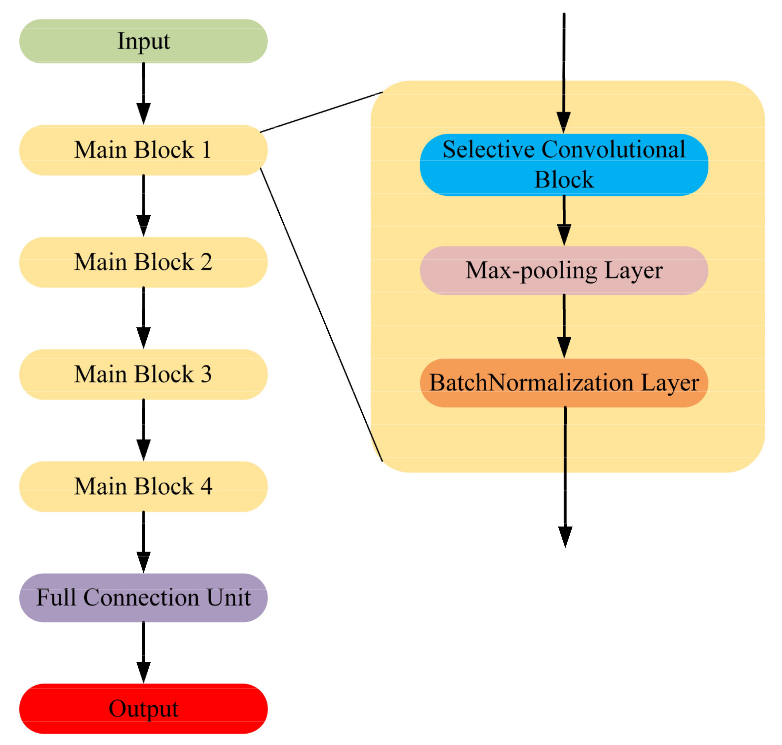
Traditional CNN models are usually designed to process 2-D data. However, the radar emitter signals are usually in 1-D form and it is time-consuming and storage-consuming to do the dimensional transformation such as time-frequency transformation. In order to improve the timeliness, in this paper, we proposed the 1-D SKCNN to classify the intra-pulse modulation of radar emitter signals. The overall architecture of the proposed 1-D SKCNN is shown in Figure 1.

Figure 1.
The overall architecture of the proposed one-dimensional selective kernel convolutional neural network (1-D SKCNN).
The input of 1-D SKCNN is the frequency-domain sequence, and this will be introduced later. There are four main blocks in 1-D SKCNN and each block contains a selective kernel convolutional block, a max-pooling layer and a batch-normalization layer [19]. Figure 2 shows the structure of the selective kernel convolutional block.
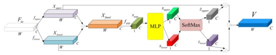
Figure 2.
The structure of selective kernel convolutional block.
In the selective kernel convolutional block, two convolutional layers are designed to extract the feature at the same time. Inspired by the fact that in the neuroscience community, the receptive field size of visual cortical neurons is modulated by the stimulus, the size of the kernel in these two convolutional layers is set to be different, which is hoped to extract the features from different scale adaptively. Assuming that is the input feature map, the calculation of the two convolutional layers with padding operation would be:
where fupper and flower are composed of two kinds of normal convolution with different size of kernel and “ReLU” activation function [20]. Then we choose addition as the fusing operation and fuse the two matrices in channel way. The fused result at this stage, could be shown as:
Like [21], we use channel-wised global-average pooling to get the global information. As the channel number of Xfused is C, the output result of global-average pooling will be a vector named . This process could be shown as:
Then xgap is sent to a Multi-Layer Perceptron (MLP) which contains a shared weight hidden layer and two independent output layer. The activation function in the shared weight hidden layer is “ReLU”. The output shape of this MLP is same as the shape of xgap. Therefore, we could get two output vector named and . This processing is shown as:
where Wshared means the weight of the shared weight hidden layer, δ means the “ReLU” function, Wupper and Wlower are the weight of two independent output layer.
Next, we choose soft attention to weight to importance of the convolutional result: Xupper and Xlower. Therefore, a SoftMax operation is applied to xupper and xlower. The process of the smoothing operation could be shown as:
where and are the corresponding smoothing result of xupper and xlower. And the final output feature map of the selective kernel convolutional block, , which is thought as the reweighted feature maps, could be obtained through the attention and the original Xupper and Xlower:
where “” stands for channel-wised elements multiply computation. Specifically, Equation (9) could be expressed as:
2.2. Preprocessing of Data
In the task of intra-pulse modulation classification of radar emitter signals, the radars may have multiple wave modes where the pulse widths could range from a microsecond to hundreds of microseconds. However, the commonly used wave mode of radars is the short pulse width mode and the pulse could be collected separately according to their pulse widths.
Therefore, assuming that the pulse widths of radar emitter signals vary in a certain range, when the sampling frequency is given, the length of the sample radar signals is determined. Unlike IQ-sampling, we sample the time-domain radar emitter signals only in one channel based on the theory of Nyquist sampling. Therefore, each pulse of radar emitter signal in analog domain will be converted to a 1-D time-domain sequence in digital domain.
CNN always requires a fixed-shaped input due to the full connection layer. As the pulse width varies in a certain range, we need to choose a suitable transformation to ensure that the input shape of each sample is the same. Although the easiest way to preprocess the data is by padding with enough zeros to ensure that the length of all preprocessed samples is the same, too many useless zeros may have a negative impact and the classification performance based on these time-domain sequences is not good. To explain this, an experiment will be introduced later.
In 1-D SKCNN, we choose to use the amplitude sequence of the signal in frequency domain as the input. First, we need to find the upper limitation of the pulse width and set a proper value of pulse width to ensure all the samples could be covered under this value. Then based on the sampling frequency, the corresponding length could be calculated. Next, we pad enough number of “0” at the end of the sampled sequence in time domain to ensure that the length of all padded sample is same. This process is shown as:
where the length of xpadded is equal to the result which is calculated by multiplying the sampling frequency and the set proper value of pulse width. refers to one of the 1-D sampled signals in time domain.
Then, we use FFT to transform xpadded and calculate the modulus of the result of FFT. This process is shown as:
where means the process of FFT. As the result, is a real sequence where the values of the elements are all greater or equal to zero. refers to the conjugation of .
To reduce the influence of different amplitudes on classification, data normalization is needed. This process is shown as:
where xinput is the input data for 1-D SKCNN. means the process of finding the max value in the sequence. Therefore, the value of each element in xinput ranges from 0 to 1.
3. Dataset and Experiments
In this section, a simulation dataset will be used to train and test the proposed method and other baseline methods. In all the experiments, a computer equipped with an Intel 10900K CPU, 64 GB RAM and RTX 3090 GPU hardware capabilities. MATLAB 2021a software, Keras and Python programming language have been used.
3.1. Dataset and Parameters Setting
Typically, the carrier frequency of radar could be from 300 MHz to 300 GHz, and it is not possible to sample those high-frequency signals directly based on the theory of Nyquist sampling. As for the receivers, they usually have adaptive local oscillators which could down mix the frequency of the received signals and output the signals with lower frequency after the low-pass filter. The output signals with lower frequency are the final signals for sampling and analyzing. Besides, relatively short pulse width mode is commonly used and it is the typical wave mode of radar.
Based on the above reasons, in this letter, we use the simulation dataset to train and test the proposed method. Eleven different varieties of radar emitter signals whose pulse widths vary from 2 μs to 50 μs, including single-carrier frequency (SCF) signals, linear frequency modulation (LFM) signals, sinusoidal frequency modulation (SFM) signals, binary frequency shift keying (BFSK) signals, quadrature frequency shift keying (QFSK) signals, even quadratic frequency modulation (EQFM) signals, dual frequency modulation (DLFM) signals, multiple linear frequency modulation (MLFM) signals, binary phase shift keying (BPSK) signals, Frank phase-coded (Frank) signals, and composite modulation (LFM-BPSK) signals. The sampling frequency is 1 GHz and the parameters of signals are shown in Table 1.

Table 1.
Parameters of radar emitter signals with eleven different intra-pulse modulations.
SNR is controlled as the power of the signals over the noise, which is defined as:
where Psignal is the power of pure radar signal and Pnoise is the power of noise. And the calculation of signal power is shown as:
where P means the power of signal, means the sampled sequence in time domain. In the simulation, the type of noise is additive white Gaussian noise (AWGN) [22] and SNR ranges from −14 dB to 0 dB with 2 dB increment. The sampled radar emitter signal with AWGN could be written as:
where means the pure sampled intra-pulse radar emitter signal sequence without noise, means the sampled AWGN, and is the sampled radar emitter signal with AWGN. Figure 3 shows the original waveforms of eleven intra-pulse modulations radar emitter signal samples in time domain when the SNR is 0 dB.
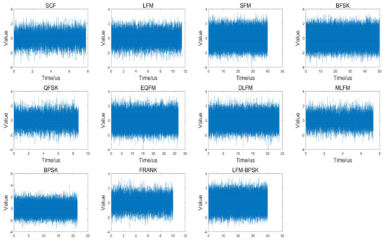
Figure 3.
The original waveforms of eleven intra-pulse modulations radar emitter signal samples in time domain when the SNR is 0 dB.
At each value of SNR, the quantity of samples for each intra-pulse modulation signal at each value of SNR is 1800, where 800 samples are used for training, 200 samples are used for validation and 800 samples are used for testing. That is, there are 70,400 samples in the training dataset, 17,600 samples in the validation dataset and 70,400 samples in the testing dataset.
The reason why the number of samples in the testing dataset is much greater than that in the validation dataset and equal to that in the training dataset is that, in real applications, the number of samples which need to be tested could be larger than that in the validation dataset. As the parameters, like carrier frequency, pulse width and bandwidth, are changing in a wider range, the testing dataset with a large number of samples could include as many situations as possible. Besides, the average classification accuracy of the well-trained model in [23] on a testing dataset containing 385,000 samples is almost 4% lower than that in a validation dataset containing 30,800 samples. Therefore, in order to increase the reliability of the classification and evaluate the real performance of the methods, we decide to use a large testing dataset. The influence of the amount of training data will be discussed in Section 3.3.4.
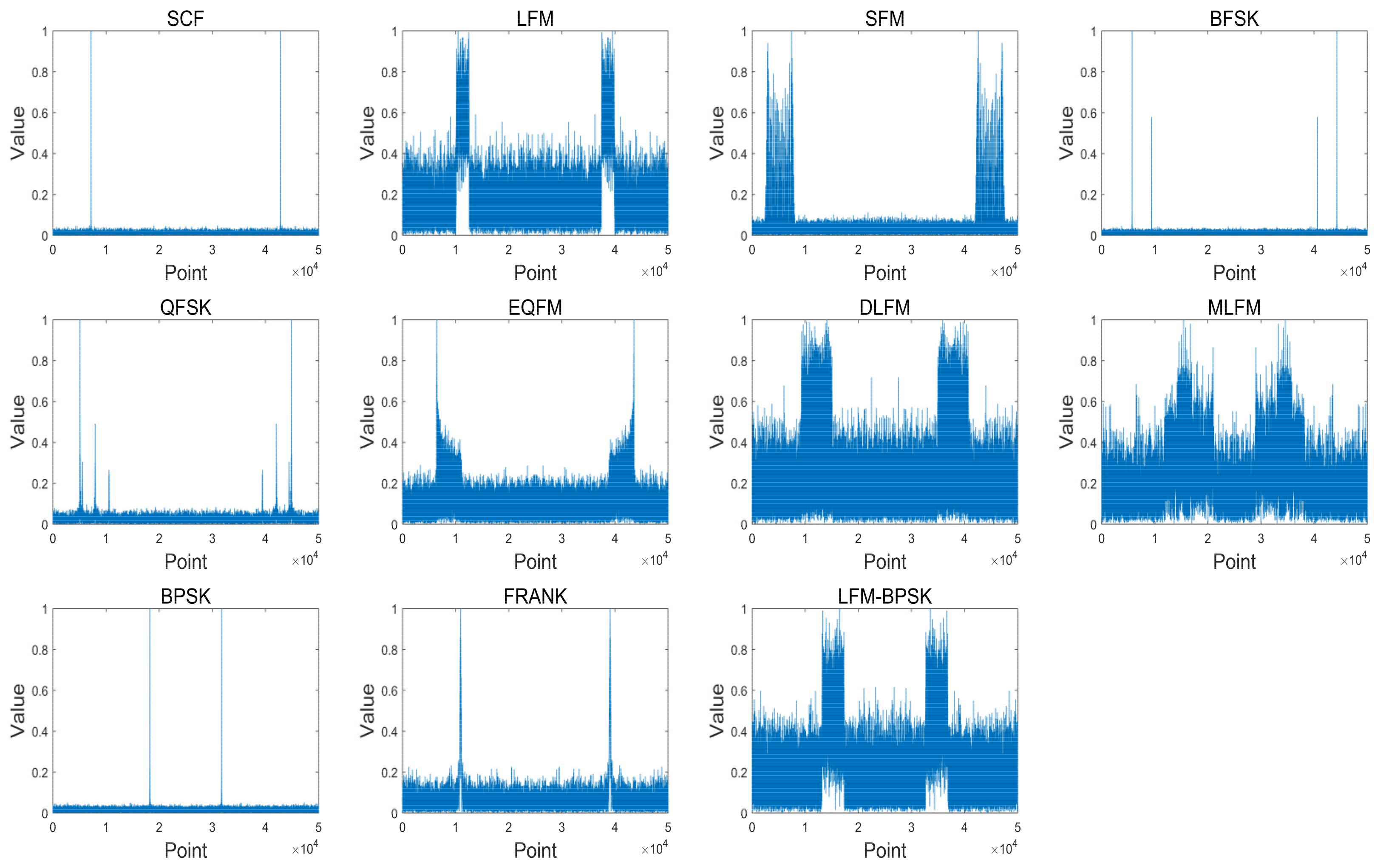
Due to the sampling frequency and the max value of pulse width, we set 50 μs as the proper value of the pulse width. Therefore, the length of xpadded in the experiment is set to 50,000. Figure 4 shows the frequency-domain amplitude spectra of the same samples in Figure 3 after data preprocessing stage.

Figure 4.
The frequency-domain amplitude spectra of the same samples in Figure 3 after data preprocessing stage where the length of xpadded is set to 50,000.
3.2. Baseline Methods
In order to provide some evidence for not choosing the time-domain sequence as the input, we use the same structure of 1-D SKCNN to conduct the experiment, which is named 1-D SKCNN-time. For this baseline method, the data preprocessing contains same zero padding (see Equation (11)) and amplitude normalization. The amplitude normalization for 1-D SKCNN-time is shown as:
where xtime is the input sequence for 1-D SKCNN-time. refers to the conjugation of xpadded.
Besides, to show the effectiveness of the selective kernel and attention mechanism, we organize three models. All three model have the same full connection layers. The structure of first two single models, named CNN-kernel_size16 and CNN-kernel_size9, are with two fixed kernel size (16 and 9, respectively) and include four blocks, where the convolutional layer, max-pooling layer and batch-normalization layer are connected one by one. And the third model named CNN-nonAP is transferred by deleting the attention part.
In addition, we employ some representative methods as the baselines including CNN-Qu [12], CNN-Kong [13], CNN-Zhang [14], GoogLeNet [17]. These methods are based on time-frequency transformation and have been proved that they have advantage of good accuracy on intra-pulse modulation classification.
3.3. Experiments on 1-D SKCNN
3.3.1. Experimental Settings of 1-D SKCNN
The two kernel sizes in the selective kernel block are 9 and 16, respectively. The pooling size and stride in each max-pooling layer are set to be 7. The full connection unit contains one hidden layer with 512 neurons and “ReLU” activation function. The activation function for the output layer is “SoftMax”.
At the stage of training 1-D SKCNN, the cross-entropy function is selected as the loss function. The optimization algorithm for the proposed 1-D SKCNN is adaptive moment estimation (ADAM) [24]. The batch size is 64 and we have run 20 epochs for training, where the learning rate in the first 15 epochs is 0.001 and in the last five epochs is 0.0001. The weights used for the testing section is saved when the accuracy of validation dataset is highest.
3.3.2. Experimental Results of 1-D SKCNN
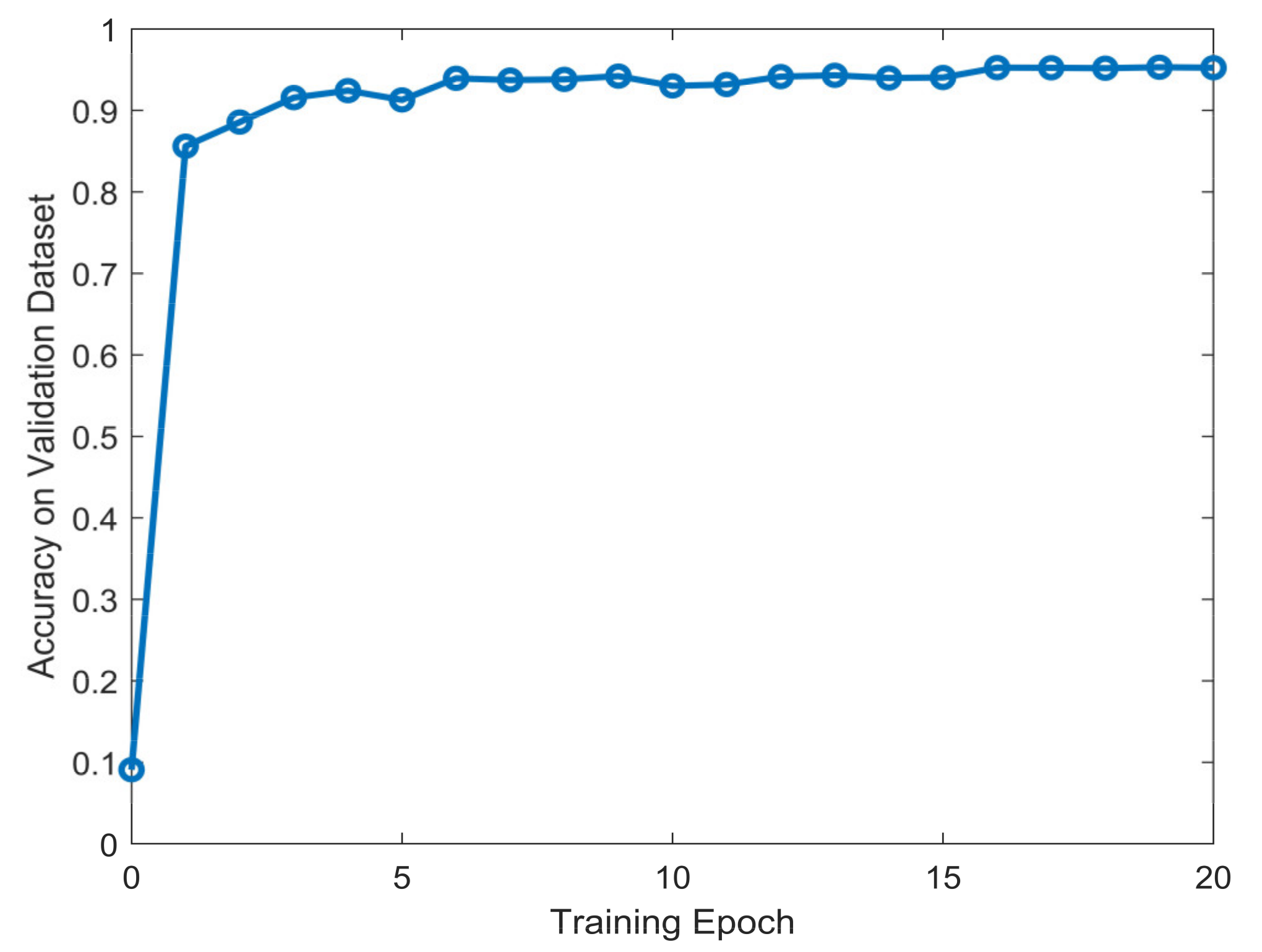
The proposed 1-D SKCNN model was trained based on the preprocessed data in Section 3.1. The value of average accuracy during the training session are shown in Figure 5.
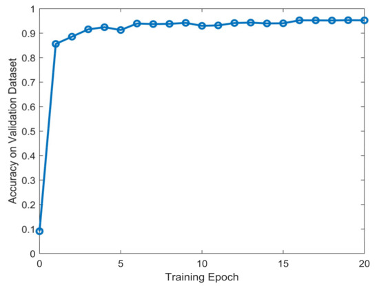
Figure 5.
The value of average accuracy on validation dataset during the training session.
Figure 5 shows that after training several epochs, the accuracy of the model on validation dataset turned to stable, which denotes that the model converged. Next, we test the classification performance of the proposed model with the weights where the accuracy of validation dataset is highest.
The classification performance under different SNR of the proposed 1-D SKCNN has been tested. Table 2 gives the classification accuracy of eleven intra-pulse modulations based on the 1-D SKCNN. When SNR is greater than or equal to −10 dB, the average classification accuracy is above 97%, and the accuracy increases as the value of SNR rises. When SNR is greater than or equal to −6 dB, the classification accuracy of each intra-pulse modulation is over 99%.
Table 2.
The classification accuracy of eleven intra-pulse modulations based on 1-D SKCNN.
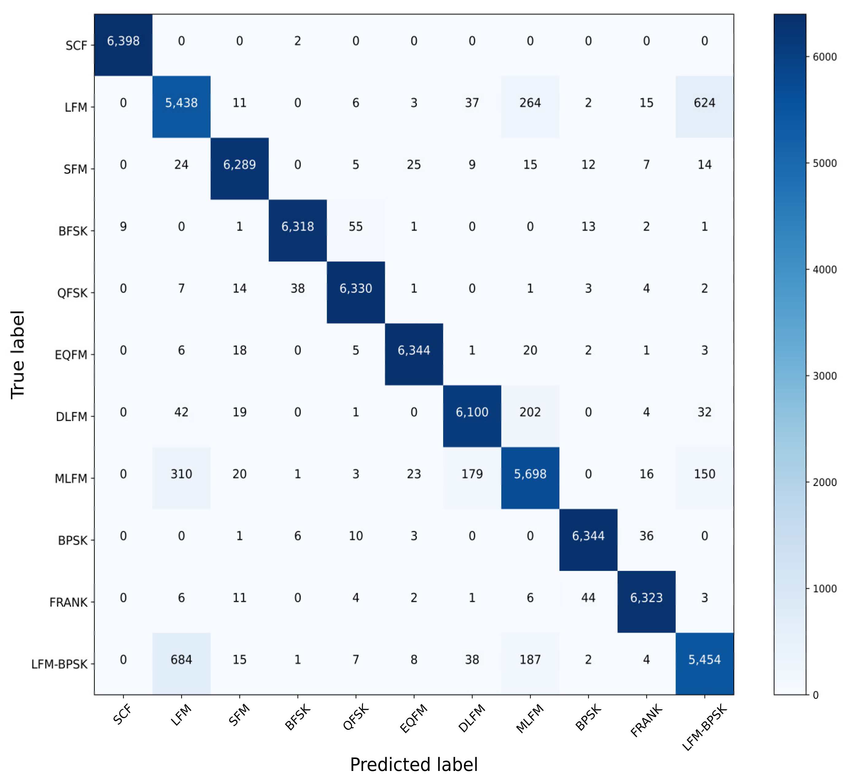
In order to analyze the specific classification result, the confusion matrix is given in Figure 6. Combined with the average accuracy in Table 2, we could find that the main errors are from the classification that some LFM signals and LFM-BPSK signals are classified mistakenly as each other. Besides, there are some DLFM signals being classified as MLFM signals, and MLFM signals being classified as LFM signals. For the other types of intra-pulse modulation signals, the 1-D SKCNN could classify them accurately even when the SNR in the extreme low condition.

Figure 6.
The confusion matrix of the classification result based on 1-D SKCNN.
3.3.3. Learned Features
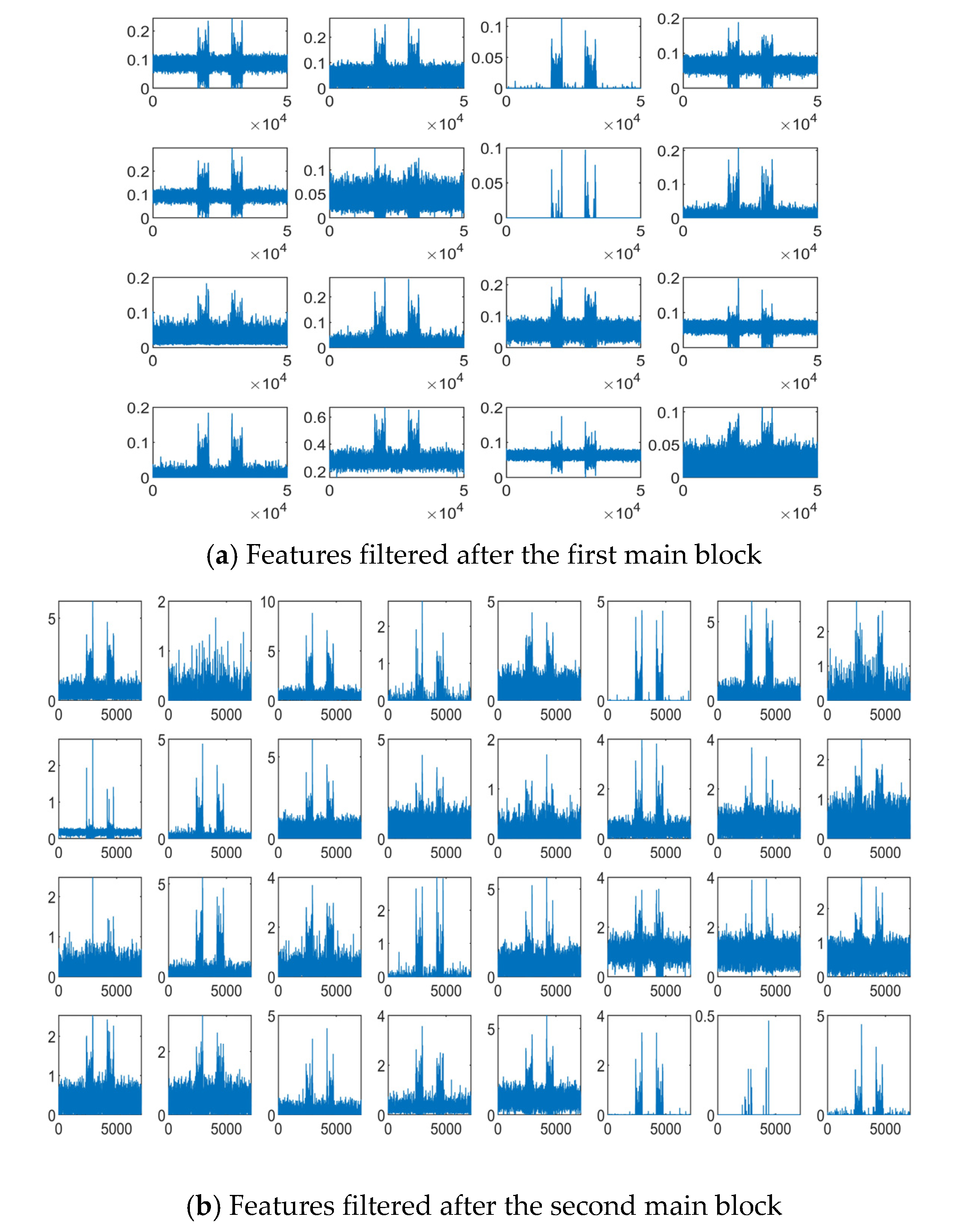
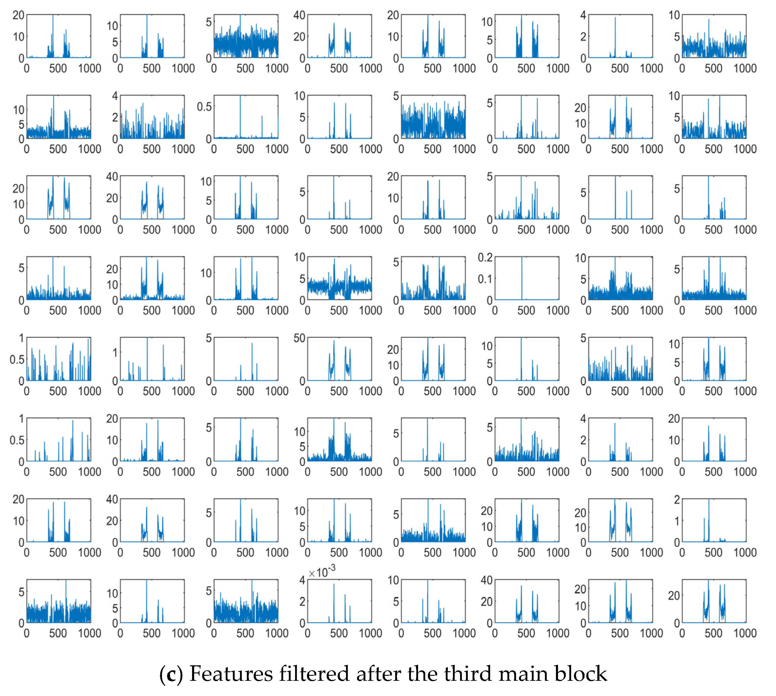
We investigate the extracted features from the proposed 1-D SKCNN. And some features filtered after the first, the second and the third main block based on one SFM sample are shown in Figure 7a–c, respectively. Figure 7 shows that as the depth of layer increases, the extracted features become sparser and more abstract, which indicates some intrinsic patterns in that SFM signal.
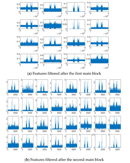
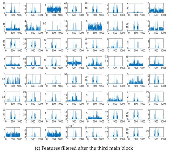
Figure 7.
Features of one SFM signal sample filtered after the first, the second and the third main block when the SNR is −10 dB.
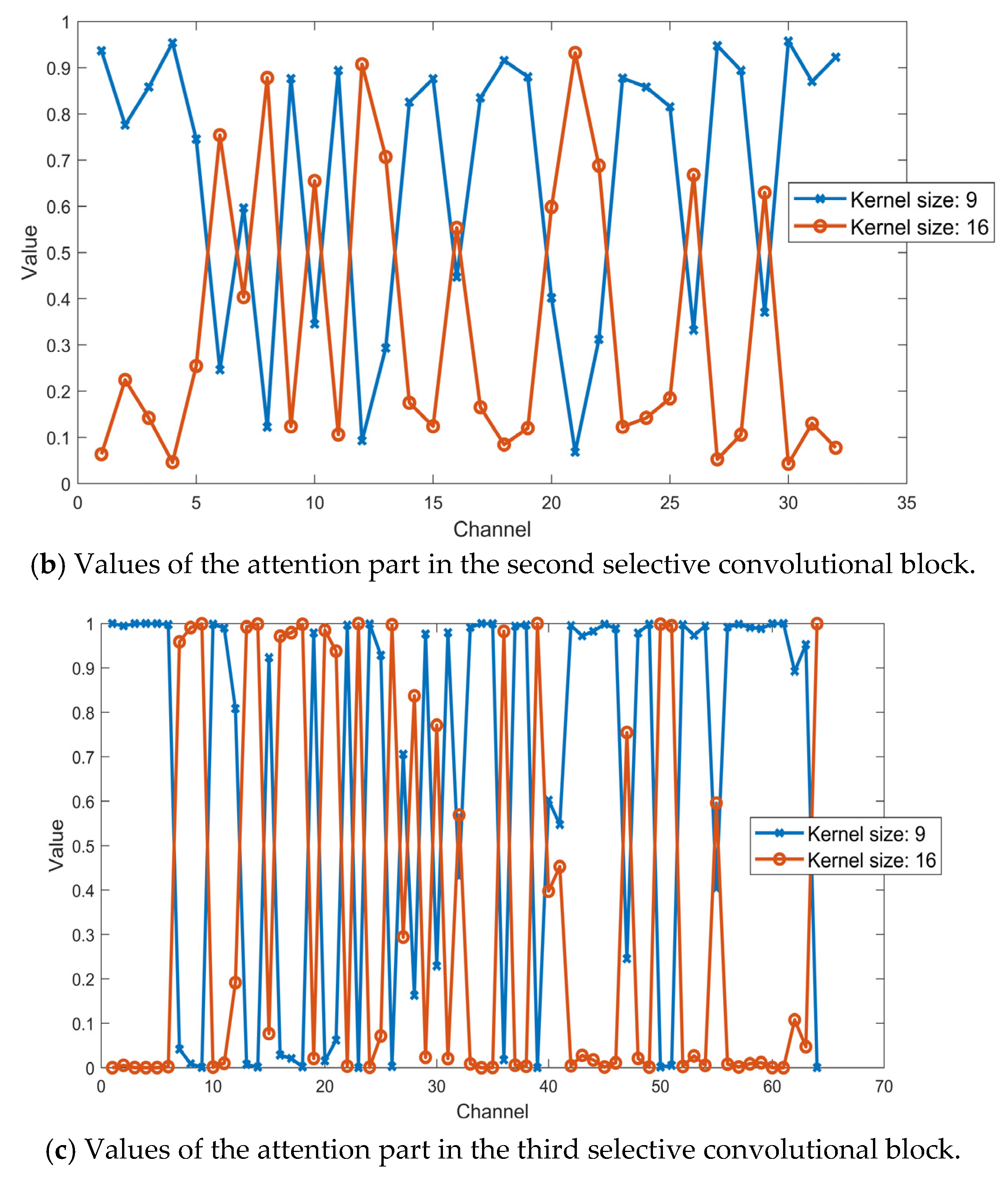
Besides, to visualize the attention part in the selective kernel convolutional blocks, we analyze the value of zupper which refers to the attention part for the kernel size 9 and zlower which refers to the attention part for the kernel size 16 by using the same SFM sample. The values of the attention part in the first, second and third selective convolutional block is shown in Figure 8a–c, respectively. It indicates that the features filtered by the convolutional layer with different kernel size are weighted by the soft-attention part. In other words, for each output channel from the selective convolutional block, it was fused from its original two channels that gain weights differently based on the attention part.
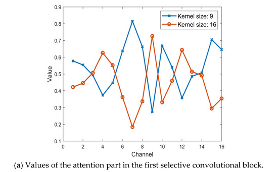

Figure 8.
Values of the attention part in the first, the second and the third selective convolutional block with the same SFM sample.
3.3.4. The Influence of Volume of Training Data Size
We investigated the performance of the proposed method with different training data sizes. The validation dataset and testing dataset are the same as before. 0%, 5%, 10%, 25%, 50%, 75% and 100% of the whole training dataset are used for training 1-D SKCNN. The weights were saved when the accuracy of validation dataset is the highest and they were used for the testing section. Figure 9 shows the average accuracy of 1-D SKCNN on testing dataset when the volume of training dataset is 0%, 5%, 10%, 25%, 50%, 75% and 100% of the original training dataset.
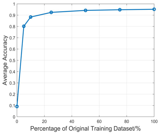
Figure 9.
The average accuracy of 1-D SKCNN on testing dataset when the volume of training dataset is 0%, 5%, 10%, 25%, 50%, 75% and 100% of the original training dataset.
As Figure 9 shows, the average accuracy of 1-D SKCNN increases logarithmically based on volume of training data size, which satisfies the conclusions in [25]. Besides it could be concluded that the scale of the original training dataset with 70,400 samples is enough for training the proposed 1-D SKCNN.
4. Comparisons with the Baselines and Discussion
In order to show the superiority of the proposed method, in this section we will compare the proposed method with the baseline methods. For the task of intra-pulse modulation classification of radar emitter signals, the process of these method mainly focus on two things: (1) Time and storage usage and (2) the classification performance. Therefore, the comparisons could be divided into two parts: (1) Comparisons among the methods in the time and storage space usage. (2) Comparisons among the methods in classification performance.
4.1. Comparisons with the Baselines in the Time and Storage Space Usage
The scale of parameter for the model is a typical feature to measure the storage space usage. As the result, we provide the parameters for each CNN model in the methods in Table 3. As the table shows, 1-D SKCNN is light-design with fewer parameters compared with the 2-D CNN based model.
Table 3.
The scale of parameter of the models in different methods.
Then, we evaluate the time usage of the methods. The time usage could be divided into two part: 1. The stage of data preprocessing. 2. The stage of training model. The data preprocessing for all methods was done by MATLAB 2021a. We randomly selected 500 samples from the dataset to do the data preprocessing for all methods, and the time usage is shown in Table 4.
Table 4.
The time usage of the methods to preprocess 500 randomly selected samples.
It is obvious that those 2-D CNN based methods which require time-frequency transformation need much more time to prepare the data for training models. And compared with the baselines, the FFT-based data preprocessing is easier to be accomplished.
Next, we evaluate the time usage in the stage of training model. Table 5 gives the time usage per training epoch which includes the validation part and the number of epoch used for training. It could be seen that 1-D CNN-based methods require more time than the 2-D CNN-based methods. The main reason for this is that the input for 1-D CNN model is a vector with the shape of 1 × 50,000. However, the input for those 2-D CNN models requiring less training time is a matrix with the shape of 64 × 64 or 128 × 128. As the result, there will be more multiplication and addition operations in 1-D CNN-based methods.
Table 5.
The time usage for training the model in different methods.
4.2. Comparisons with the Baselines in the Classification Performance
In this section, we will evaluate the classification performance of the methods with different evaluation metrics, including average accuracy (AA), kappa coefficient (KC), recall, precision and F1-score. Table 6 gives the classification accuracy of different methods on the testing dataset and the KC, the recall, the precision and the F1-score are given in Table 7.
Table 6.
The time usage for training the model in different methods.
Table 7.
The time usage for training the model in different methods.
The comparison between 1-D SKCNN-time and 1-D SKCNN shows that although the structure of the model is the same, the frequency-domain sequence, instead of time-domain sequence, could bring a much positive classification result when it is used as the input. Then, except for 1-D SKCNN-time, we find that the classification performance of 1-D CNN-based methods are superior to those 2-D TFI-based CNN methods based on the given metrics. Although GoogleNet performs best among the 2-D CNN methods and its classification accuracy could be near to 100% when SNR is high, its rate of accuracy falls faster when compared with other 1-D CNN-based method except 1-D SKCNN-time. And when SNR is −10 dB, all of the 1-D CNN model except 1-D SKCNN-time could remain a good classification accuracy with over 90%.
Besides, the comparisons among 1-D SKCNN, CNN-kernel_size16, CNN-kernel_size9 and CNN-nonAP show that 1-D SKCNN performs best not only in the overall average accuracy, but also in every condition of SNR. And based on the analysis of time and storage usage in Section 4.1, we could find that the selective kernel convolutional blocks, which contain selective kernel convolutional layers and soft-attention part at the same time, cost little computation resource and could provide a better classification result.
5. Conclusions
In this paper, we have proposed 1-D SKCNN for intra-pulse modulation classification of radar emitter signals. The proposed method uses a 1-D frequency-domain sequence as input, which has the advantage of fast speed in the stage of data preprocessing. The comparisons with the baseline methods in both time, storage usage and classification performance show that the proposed method, which employs selective kernel convolutional layers and a soft-attention part at the same time, has superior performance in intra-pulse modulation classification of radar emitter signals under various SNR scenarios.
Author Contributions
Conceptualization, S.Y. and B.W.; methodology, S.Y. and B.W.; software, S.Y.; validation, S.Y.; formal analysis, B.W. and S.Y.; investigation, S.Y. and B.W.; resources, B.W.; data curation, S.Y.; writing—original draft preparation, S.Y.; writing—review and editing, S.Y.; supervision, P.L. All authors have read and agreed to the published version of the manuscript.
Funding
This research received no external funding.
Data Availability Statement
Data sharing not applicable.
Acknowledgments
The author would like to show their gratitude to the editors and the reviewers for their insightful comments.
Conflicts of Interest
The authors declare no conflict of interest.
References
- Barton, D.K. Radar System Analysis and Modeling; Artech: London, UK, 2004. [Google Scholar]
- Richards, M.A. Fundamentals of Radar Signal Processing, 2nd ed.; McGraw-Hill Education: New York, NY, USA, 2005. [Google Scholar]
- Wiley, R.G.; Ebrary, I. ELINT: The Interception and Analysis of Radar Signals; Artech: London, UK, 2006. [Google Scholar]
- Yang, C.; He, Z.; Peng, Y.; Wang, Y.; Yang, J. Deep Learning Aided Method for Automatic Modulation Recognition. IEEE Access 2019, 7, 109063–109068. [Google Scholar] [CrossRef]
- Park, C.-S.; Choi, J.-H.; Nah, S.-P.; Jang, W.; Kim, D.Y. Automatic Modulation Recognition of Digital Signals using Wavelet Features and SVM. In Proceedings of the 9th International Conference on Advanced Communication Technology, Gangwon, Korea, 12–14 February 2007; Volume 1, pp. 387–390. [Google Scholar] [CrossRef]
- Schmidhuber, J. Deep learning in neural networks: An overview. Neural Netw. 2015, 61, 85–117. [Google Scholar] [CrossRef] [PubMed] [Green Version]
- Krizhevsky, A.; Sutskever, I.; Hinton, G. ImageNet Classification with Deep Convolutional Neural Networks; Curran Associates Inc.: New York, NY, USA, 2012. [Google Scholar]
- Szegedy, C.; Liu, W.; Jia, Y.; Sermanet, P.; Reed, S.; Anguelov, D.; Erhan, D.; Vanhoucke, V.; Rabinovich, A. Going Deeper with Convolutions. In Proceedings of the IEEE Conference on Computer Vision and Pattern Recognition (CVPR), Boston, MA, USA, 7–12 June 2015; pp. 1–9. [Google Scholar]
- Srivastava, R.K.; Greff, K.; Schmidhuber, K. Highway networks. arXiv 2015, arXiv:1505.00387. [Google Scholar]
- He, K.; Zhang, X.; Ren, S.; Sun, J. Deep Residual Learning for Image Recognition. In Proceedings of the 2016 IEEE Conference on Computer Vision and Pattern Recognition (CVPR), Las Vegas, NV, USA, 27–30 June 2016; pp. 770–778. [Google Scholar] [CrossRef] [Green Version]
- Huang, G.; Liu, Z.; van der Maaten, L.; Weinberger, K.Q. Densely connected convolutional networks. In Proceedings of the IEEE Conference on Computer Vision and Pattern Recognition (CVPR), Honolulu, HI, USA, 21–26 July 2017; pp. 2261–2269. [Google Scholar] [CrossRef] [Green Version]
- Qu, Z.; Mao, X.; Deng, Z. Radar Signal Intra-Pulse Modulation Recognition Based on Convolutional Neural Network. IEEE Access 2018, 6, 43874–43884. [Google Scholar] [CrossRef]
- Kong, S.-H.; Kim, M.; Hoang, L.M.; Kim, E. Automatic LPI Radar Waveform Recognition Using CNN. IEEE Access 2018, 6, 4207–4219. [Google Scholar] [CrossRef]
- Zhang, J.; Li, Y.; Yin, J. Modulation classification method for frequency modulation signals based on the time—Frequency distribution and CNN. IET Radar Sonar Navig. 2018, 12, 244–249. [Google Scholar] [CrossRef]
- Liu, Z.; Shi, Y.; Zeng, Y.; Gong, Y. Radar Emitter Signal Detection with Convolutional Neural Network. In Proceedings of the 2019 IEEE 11th International Conference on Advanced Infocomm Technology (ICAIT), Jinan, China, 18–20 October 2019; pp. 48–51. [Google Scholar] [CrossRef]
- Wang, F.; Yang, C.; Huang, S.; Wang, H. Automatic modulation classification based on joint feature map and convolutional neural network. IET Radar Sonar Navig. 2019, 13, 998–1003. [Google Scholar] [CrossRef]
- Yu, Z.; Tang, J.; Wang, Z. GCPS: A CNN Performance Evaluation Criterion for Radar Signal Intrapulse Modulation Recognition. IEEE Commun. Lett. 2021. [Google Scholar] [CrossRef]
- Li, X.; Wang, W.; Hu, X.; Yang, J. Selective Kernel Networks. In Proceedings of the 2019 IEEE/CVF Conference on Computer Vision and Pattern Recognition (CVPR), Long Beach, LA, USA, 15–21 June 2019; pp. 510–519. [Google Scholar]
- Ioffe, S.; Szegedy, C. Batch normalization: Accelerating deep network training by reducing internal covariate shift. arXiv 2015, arXiv:1502.03167. [Google Scholar]
- Nair, V.; Hinton, G.E. Rectified linear units improve restricted boltzmann machines. In Proceedings of the 27th International Conference on Machine Learning (ICML-10), Haifa, Israel, 21–24 June 2010. [Google Scholar]
- Hu, J.; Shen, L.; Albanie, S.; Sun, G.; Wu, E. Squeeze-and-Excitation Networks. IEEE Trans. Pattern Anal. Mach. Intell. 2020, 42, 2011–2023. [Google Scholar] [CrossRef] [PubMed] [Green Version]
- Hoang, L.M.; Kim, M.; Kong, S.-H. Automatic Recognition of General LPI Radar Waveform Using SSD and Supplementary Classifier. IEEE Trans. Signal Process. 2019, 67, 3516–3530. [Google Scholar] [CrossRef]
- Wu, B.; Yuan, S.; Li, P.; Jing, Z.; Huang, S.; Zhao, Y. Radar Emitter Signal Recognition Based on One-Dimensional Convolutional Neural Network with Attention Mechanism. Sensors 2020, 20, 6350. [Google Scholar] [CrossRef] [PubMed]
- Kingma, D.P.; Ba, J. Adam: A Method for Stochastic Optimization. arXiv 2014, arXiv:1412.6980. [Google Scholar]
- Sun, C.; Shrivastava, A.; Singh, S.; Gupta, A. Revisiting unreasonable effectiveness of data in deep learning era. In Proceedings of the 16th IEEE International Conference on Computer Vision (ICCV), Venice, Italy, 22–29 October 2017. [Google Scholar]


Publisher’s Note: MDPI stays neutral with regard to jurisdictional claims in published maps and institutional affiliations. |
© 2021 by the authors. Licensee MDPI, Basel, Switzerland. This article is an open access article distributed under the terms and conditions of the Creative Commons Attribution (CC BY) license (https://creativecommons.org/licenses/by/4.0/).