Article

Convolutional Neural Network with a Learnable Spatial Activation Function for SAR Image Despeckling and Forest Image Analysis

1
School of Electronic and Optical Engineering, Nanjing University of Science and Technology, Nanjing 210094, China
2
College of Information Science and Technology, Nanjing Forestry University, Nanjing 210037, China
*
Author to whom correspondence should be addressed.
Remote Sens. 2021, 13(17), 3444; https://doi.org/10.3390/rs13173444
Submission received: 29 June 2021 / Revised: 13 August 2021 / Accepted: 26 August 2021 / Published: 30 August 2021
(This article belongs to the Special Issue Terrestrial Laser Scanning of Forest Structure)

Abstract

:
Synthetic aperture radar (SAR) images are often disturbed by speckle noise, making SAR image interpretation tasks more difficult. Therefore, speckle suppression becomes a pre-processing step. In recent years, approaches based on convolutional neural network (CNN) achieved good results in synthetic aperture radar (SAR) images despeckling. However, these CNN-based SAR images despeckling approaches usually require large computational resources, especially in the case of huge training data. In this paper, we proposed a SAR image despeckling method using a CNN platform with a new learnable spatial activation function, which required significantly fewer network parameters without incurring any degradation in performance over the state-of-the-art despeckling methods. Specifically, we redefined the rectified linear units (ReLU) function by adding a convolutional kernel to obtain the weight map of each pixel, making the activation function learnable. Meanwhile, we designed several experiments to demonstrate the advantages of our method. In total, 400 images from Google Earth comprising various scenes were selected as a training set in addition to 10 Google Earth images including athletic field, buildings, beach, and bridges as a test set, which achieved good despeckling effects in both visual and index results (peak signal to noise ratio (PSNR): 26.37 ± 2.68 and structural similarity index (SSIM): 0.83 ± 0.07 for different speckle noise levels). Extensive experiments were performed on synthetic and real SAR images to demonstrate the effectiveness of the proposed method, which proved to have a superior despeckling effect and higher ENL magnitudes than the existing methods. Our method was applied to coniferous forest, broad-leaved forest, and conifer broad-leaved mixed forest and proved to have a good despeckling effect (PSNR: 23.84 ± 1.09 and SSIM: 0.79 ± 0.02). Our method presents a robust framework inspired by the deep learning technology that realizes the speckle noise suppression for various remote sensing images.

1. Introduction

With the development of radio technology, radar has not only been used in military fields such as target detection [1,2] and reconnaissance [3,4] but also plays an important role in weather forecasting [5], environmental protection [6,7], etc. Synthetic aperture radar (SAR) [8,9] is an efficient type of radar system, which can generate high resolution images on the moving platform, such as airplanes, satellites, etc. In the process of radar movement, the ground target is scanned by transmitting electromagnetic waves and reflects the radar echo signal. Finally, the radar image is synthesized by the collected two-dimensional echo signal.
Compared with optical and infrared imaging systems, SAR possesses inherent all-day and all-weather acquisition capability and makes some difficult tasks possible, such as detecting hidden targets and interferometry [10,11]. However, the SAR images are often inhibited by speckle, which is formed by the interference echo of each resolution cell and brings the difficulties for SAR images processing and interpretation. Therefore, the image despeckling is crucial and is used as a pre-processing step in various SAR applications [12,13].
For SAR images, the main reason for contamination is multiplicative speckle noise, and this noise model can be described by the following equation.
Y = X N
where Y denotes the observed intensity image with size of W × H, X is the clean image with size of W × H corresponding to the Y, and N represents the factor of speckle noise. Specifically, for SAR amplitude image, N follows a Gamma distribution with unit mean and variance 1/L and has the following distribution [14]:
P ( N ) = L L N L 1 exp ( N L ) Γ ( L )
where L ≥ 1, N ≥ 0, Γ ( ) denotes the Gamma function, and L is the equivalent number of looks (ENL). The purpose of speckle suppression methods based on the convolutional neural network is to learn the nonlinear mapping relationships between clean images and corresponding noisy images.
Since the 1980s, different methods for despeckling have been proposed based on various technologies, such as multilook processing [15,16,17,18], spatial domain filters [19,20,21,22], wavelet transform [23,24,25,26], nonlocal filtering [27,28,29,30], and total variation [31,32,33,34]. The multilook processing can suppress speckle noise simply and effectively, but this leads to reduction of resolution for SAR image. Spatial domain filtering methods can effectively suppress noise, but they always have the problem of excessive smoothing of edge and detail information. Wavelet transform based methods are superior to the spatial domain filtering methods in speckle suppression. However, these kinds of methods still cannot save the texture details of the image effectively. The methods based on the non-local idea, such as probabilistic patch-based (PPB) [28] and SAR block-matching 3D (SAR-BM3D) [29], can achieve better results for speckle suppression and texture information. The basic idea is that there are large numbers of similar blocks in the whole image, and the self-similarity between the blocks is employed. However, the search for similar blocks increases the computational complexity for non-local methods. Although the above methods have achieved good results for despeckling, some of these methods still face problems if the intention is to preserve excellent detailed features in domains of complicated texture.
In recent years, with the development of computer hardware, various methods based on deep convolutional neural networks were successfully applied in image denoising tasks [35]. Compared with traditional algorithms for SAR image despeckling, a deep neural network is more powerful to solve complex non-linear problems. Chierchia [36] used homomorphic processing and residual learning [37] to train a convolutional neural network, in which the log-transformed images were trained in the neural network. Wang proposed a despeckling network named image despeckling convolutional neural network (ID-CNN) by using a component-wise division-residual layer to estimate speckle [38]. Zhang [39] combined skip connection [40] and dilated convolution [41] to achieve SAR despeckling. Similarly, Gui [42] proposed a network using dilated convolution and a densely connected network [43]. Lattari [44] successfully used the U-Net CNN architecture for SAR image speckle suppression. Moreover, some scholars also proposed the SAR image despeckling schemes by combining CNN with other methods, such as nonlocal methods [45,46,47] and guided filtering (GFF) methods [48,49,50]. Although CNN based methods have achieved successful despeckling application, one problem is that the despeckling network becomes deeper and wider, which leads to large computation in both network training and the despeckling process. In order to reduce network parameters, we proposed a method using a new learnable spatial activation function based on xUnit [51]. In the case of the same parameter quantity, the activation function can obtain better despeckled results than the commonly used functions such as the rectified linear unit. Moreover, the function can achieve the same performance as the original structure with fewer layers so that more complex network structural characteristics can be avoided.
In this study, we aimed to use a better convolutional neural network method for speckle suppression of SAR images. Therefore, a speckle suppression method of SAR images based on a learning activation function was introduced. In order to improve the speckle suppression performance and reduce the occupancy rate of computing resources as much as possible, an activation function with learnable parameters was proposed from the perspective of the threshold unit of ReLU, a common activation function. In order to analyze the performance of the activation function, comparative experiments were designed. The innovation of this paper is as follows: firstly, a novel algorithm is proposed to achieve speckle suppression; secondly, a complete set of experimental methods and systems is formed from theory to simulation and then to the application of real SAR images; thirdly, the method proposed in this paper not only is applicable to SAR images but also introduces forest image denoising for comparison.
The rest of the paper is organized as follows. Section 2 introduces the proposed scheme, including the network architecture, the modified xUnit (M-xUnit), and the evaluation index of SAR image speckle suppression. The results on synthetic and real SAR images are shown and compared with other state-of-art methods in Section 3. Section 4 derives the discussion and the conclusion in Section 5.

2. The Theory and Method

2.1. Structure Design of Learnable Activation Function

Convolution operation and pooling operation in convolution neural networks are linear operations, which only can solve linear problems. However, most of the practical problems are nonlinear. If just stacking the convolution layer and the pooling layer directly, the neural network will only be suitable for the linear problem. This is why CNN needs to add an activation function layer whose role is to inject nonlinear factors into the neural network so that the network can fit all kinds of curves and be able to handle practical problems. The common activation functions are as follows: logistic function (also known as Sigmoid function) [52], hyperbolic tangent function (Tanh) [53], and rectified linear units (ReLU) [54]. The expressions of the three functions are as follows:
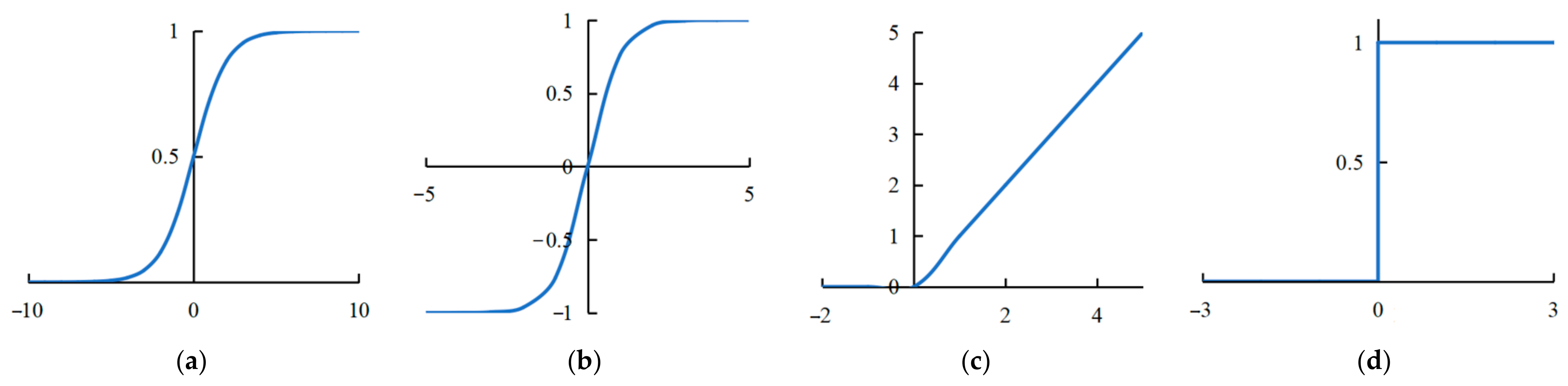
f Sigmoid x = 1 1 + exp x , f Tanh x = 1 exp 2 x 1 + exp 2 x , f ReLU x = max 0 , x .
It can be seen from Figure 1 that the Sigmoid function can compress the input signal into the interval [0, 1] [52]. Since the data are compressed to the interval [0, 1], this function is mainly used to transform the input into a form of probability that also ranges from 0 to 1. However, when the input is large or small enough, the output approaches 1 or 0 after compression, which results in gradient dispersion. The Tanh function can be obtained by scaling and translating the Sigmoid function [53]. The mean value of the Tanh is 0, and its convergence speed is faster than that of the Sigmoid function, but it still cannot solve the problem of gradient vanishing. Therefore, the ReLU function is the most commonly used activation function, which has strong sparsity and greatly reduces the number of parameters. In addition, the ReLU function solves the problem of gradient vanishing in the positive interval, and its convergence speed is much faster than the Sigmoid and the Tanh functions. However, the ReLU function is difficult to update for some parameters in the negative interval. To solve the above mentioned problems, there are also some improved versions of ReLU functions, such as the parametric rectified linear unit (PReLU), ELU, etc. These improved functions exist to make up for the defects of the ReLU function.
Although there are different kinds of convolutional neural network structures, their structures are basically similar, mainly composed of convolution and activation functions. From a mathematical point of view, the relationship between layer k and layer k + 1 is as follows:
z k = W k x k + b k , x k + 1 = f z k .
where x is the k-layer input, Wk is the convolution operation, bk is the bias term, f (·) is the nonlinear activation function, and xk+1 is the layer input.
Taking the ReLU activation function as an example, the nonlinear operation of the function satisfies f (0) = 0, and the input of layer k + 1 in Equation (4) can be converted into:
x k + 1 = z k g k
The symbol in the formula is the Hadamard product, that is, the product of the corresponding elements of two matrices. gk represents the weight mapping related to zk, which is defined as follows:
g k i = f z k i z k i
where gk is 0 when zk is 0.
The ReLU curve in Figure 1c is derived, and the following formulas can be obtained:
f z k = z k       z k > 0 , f z k = 0         z k 0 .
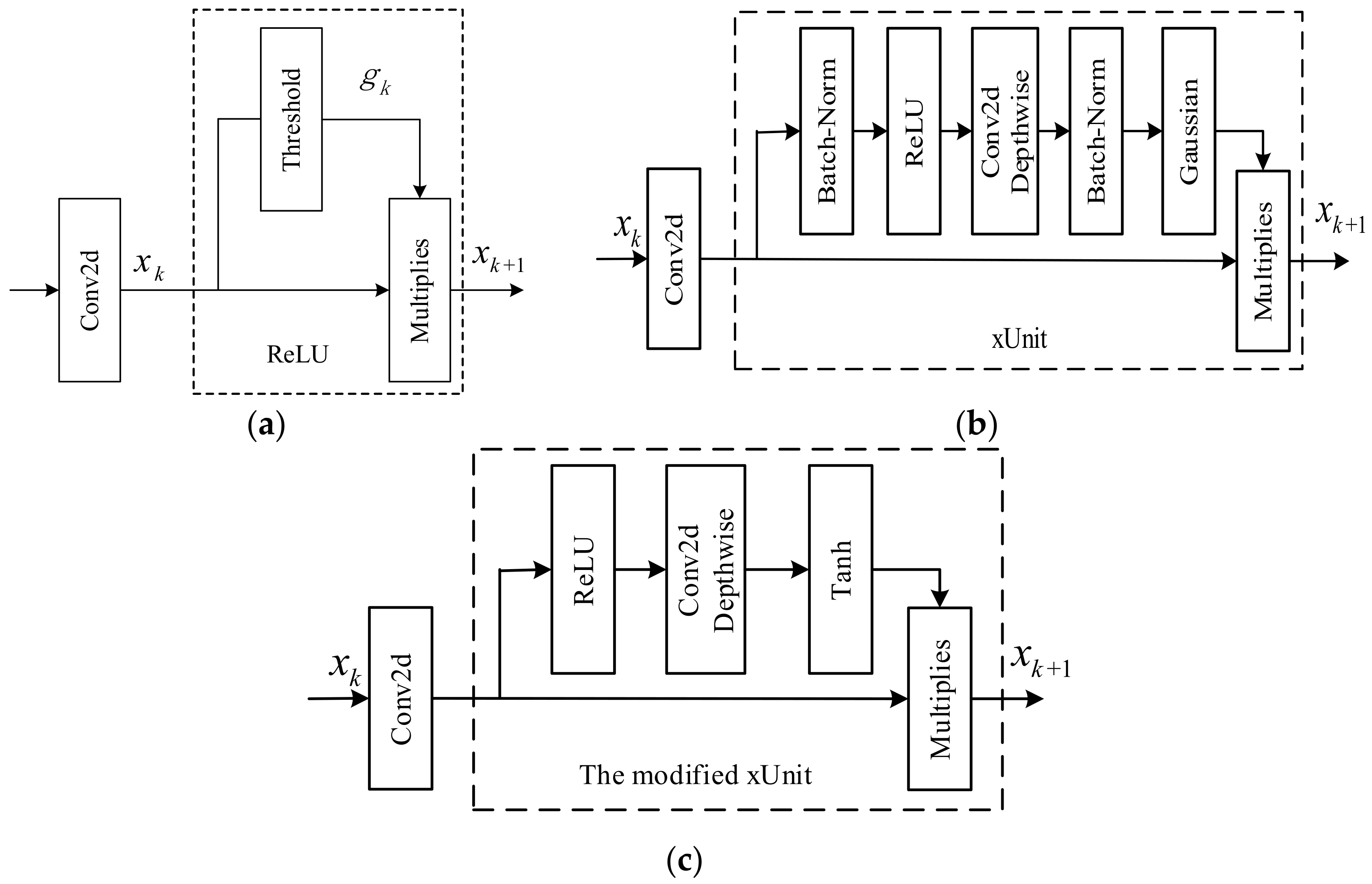
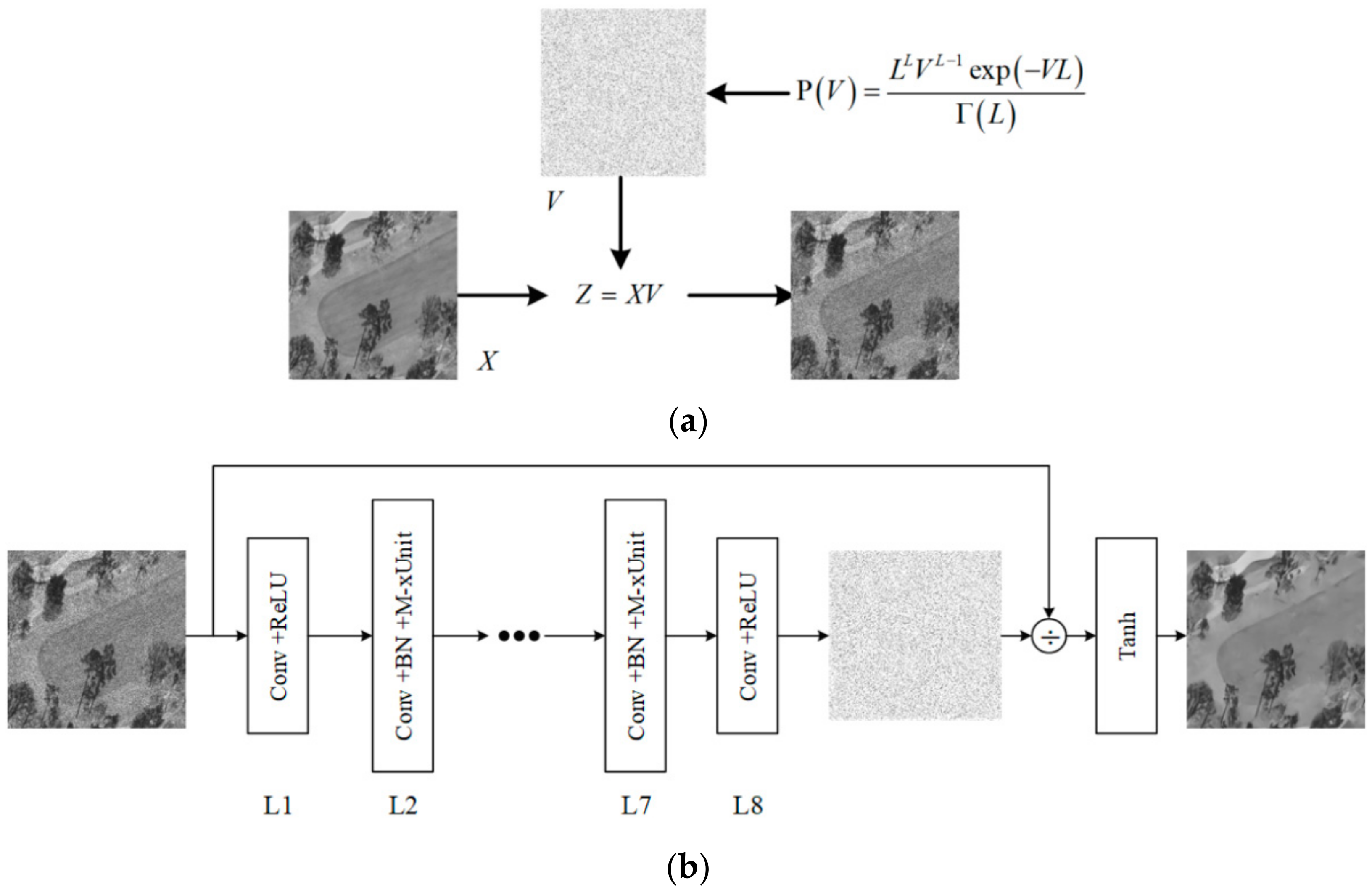
Although the CNNs of various complex structures are proposed to improve the denoising performance in SAR image speckle suppression tasks, these network structures cannot avoid a large number of network parameters. Here, a modified xUnit activation is proposed and incorporated into ID-CNN structure to further improve the denoising performance. According to the characteristics of the ReLU shown in Figure 1c, a ReLU derivative curve shown in Figure 1d can be obtained. At this point, the ReLU activation function can be considered as a threshold unit (0 or 1) shown in Figure 2a, where gk denotes the threshold unit (0 or 1), and xk and xk+1 respectively represent the ReLU functions of input and output. By contrast, a learnable spatial activation function is proposed to construct a weight map in the range [0, 1] so that each element is related to the spatial neighborhood of its corresponding input element [51].
It can deduce that gk is a threshold unit related to zk. The formula is as follows:
g k i = 1       z k i > 0 , 0       z k i 0 .
Equation (8) represents the redefined ReLU activation function, and its structure is shown in Figure 2a. Multiplies represents the product of corresponding elements, namely the Hadamard product.
As can be seen from Figure 2a, the input xk is convoluted to get zk. The ReLU function can be regarded as setting the threshold unit gk value according to each element value of zk and multiplying it to get the output xk+1.
According to Figure 2a, the gk value of the M-xUnit function in this section is not only related to the corresponding element of zk but is also related to the spatial adjacent elements. The basic idea is to construct a weight mapping in which the weight of each element depends on the corresponding spatial adjacent input elements. This relationship can be realized by convolution operation. As shown in Figure 2c, the constructed weight mapping realizes nonlinear operation through a ReLU activation function, then successively going through the deep convolution and the Tanh function, and, finally, the weight range is mapped between [−1, 1]. Among these operations, the employment of deep convolution ensures that the weight of each element is related to its corresponding spatial adjacent elements. The introduction of Tanh solves the problem that the output of ReLU is not zero-centered and makes up for the defect that the element value is zero by ReLU when it is less than or equal to zero, which avoids the phenomenon that some units will never be activated.
In Figure 2c, gk of M-xUnit activation unit is defined as:
g k i = Tanh d k i , d k i = H k ReLU [ z k ] i .
where Hk represents deep convolution, while dk represents the output of deep convolution.
To enable xUnit shown in Figure 2b to perform better in the ID-CNN architecture and the task of SAR despeckling, the Gaussian function was replaced with a hyperbolic tangent function (Tanh), and two batch normalization (BN) [55] layers were removed. Tanh function can map the dynamic range to [−1, 1] so that the mean value of the output distribution is zero and resembles the identity function when input remains around zero. As shown, the BN layers cannot improve the denoising performance of the SAR image, and the possible reason is that the output of the hidden layer is normalized by BN, which destroys the distribution of the original space [39,56]. The modified xUnit is shown in Figure 2c, where Conv2d represents the operation of convolution, and Conv2d Depthwise denotes deep convolution [57] whose kernel size is set as 9 × 9.
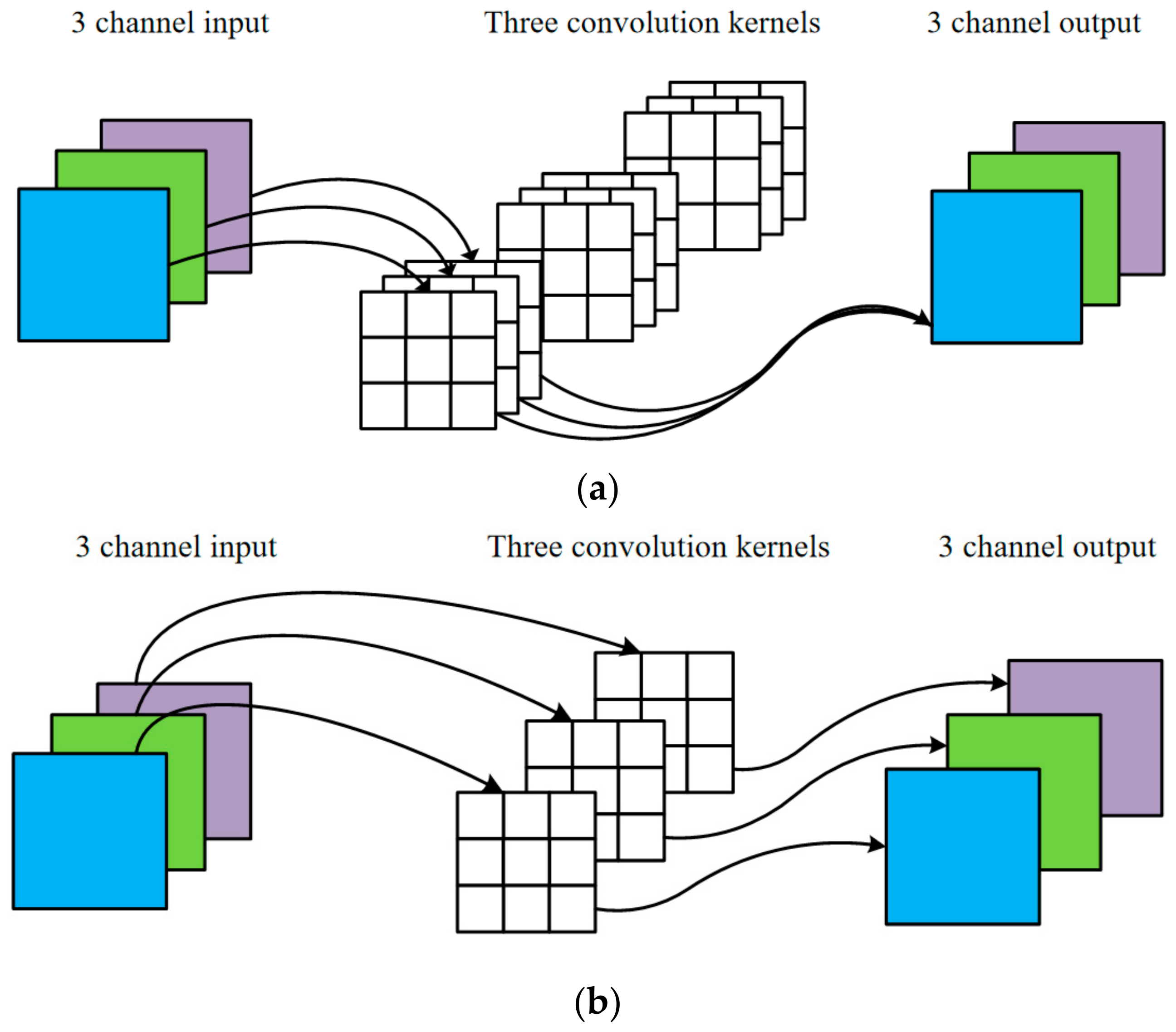
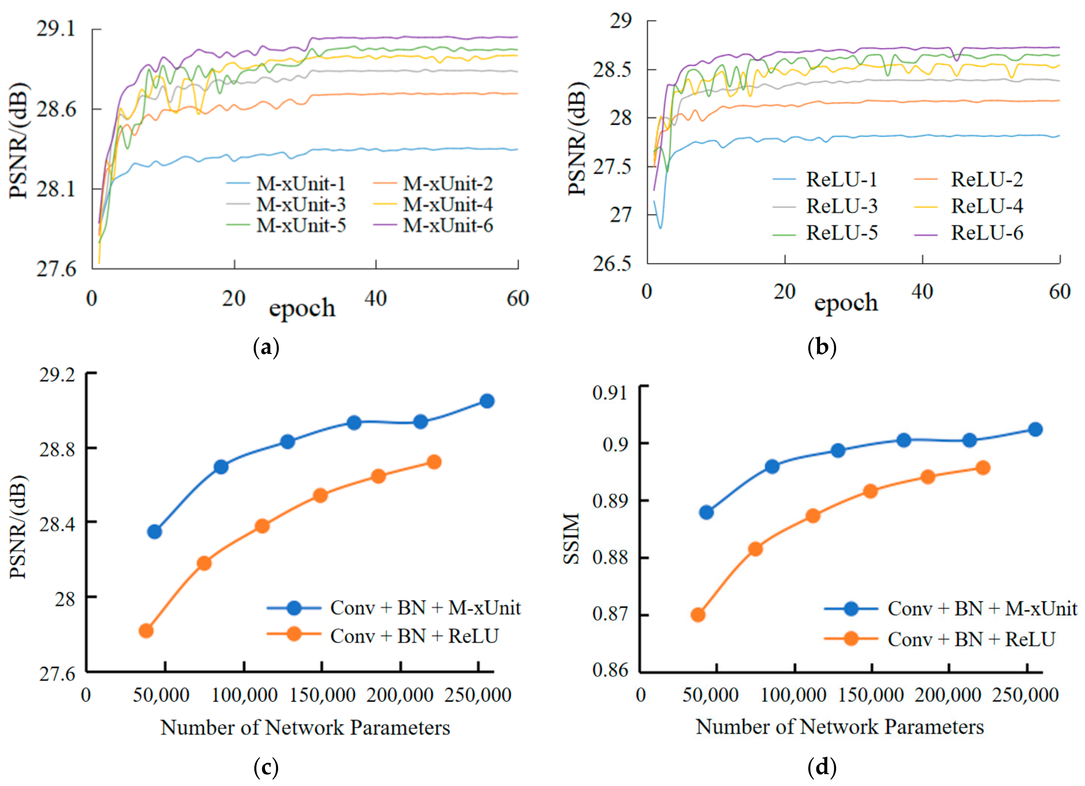
Figure 3 shows the difference between deep convolution and ordinary convolution. One convolution kernel of deep convolution corresponds to one channel, and each channel can only be convoluted by one kernel. The number of output channels generated in this process is the same as the number of input channels. Compared with ordinary convolution, deep convolution has lower parameters and lower operation cost, which is the main reason why M-xUnit has fewer parameters. Although the number of parameters for a function increases, compared with the parameters of the whole network, the increase of parameters is quite limited. At the same time, the speckle suppression performance of the network is also improved.
Assume the size of the input image is M × N with m channels, the size of the convolution kernel is k × k , and the number of kernels is n. As is shown in Figure 3, for ordinary convolution, each output channel is convoluted by m kernels, thus the computational complexity is M × N × k × k × m × n , while for deep convolution, each output channel is convoluted by only one kernel, thus its computational complexity is M × N × k × k × n . It can be seen that the computation cost of deep convolution is 1 / m times that of ordinary convolution.
However, deep convolution cannot expand the feature maps, and because the input channels are convoluted separately, it cannot effectively use the feature information of different channels in the same spatial position. Therefore, it is necessary to employ pointwise convolution to combine the feature maps generated by deep convolution into a new feature map. The combination of the two convolutions forms a deep separable convolution, which is very suitable for the lightweight network of the mobile terminal. This is also the core of Mobilenet [57] and Xception [58]. However, the basic idea of the M-xUnit activation function in this section is to correlate the weight mapping with the corresponding spatial adjacent elements of the input elements. This only requires a convolution operation and does not need to consider whether or not to effectively use the feature information of the same spatial position between channels. Therefore, this section only adds one layer of deep convolution to the M-xUnit activation unit.

2.2. Loss Function

Loss function is the basic and critical factor and can measure the prediction effect of a model [59,60]. It can be effectively applied to various tasks of deep learning through the definition and the optimization of loss function. In Section 2.2, the combination of Euclidean loss and TV loss as a loss function is used. Specifically, the Euclidean loss is used to minimize the error between the estimated image and the target image. Moreover, the TV loss is used to smooth the predicated image. They are defined as:
L E = 1 W H w = 1 W h = 1 H X ˜ w , h X w , h 2 2
L T V = w = 1 W h = 1 H X ˜ w + 1 , h X ˜ w , h 2 + X ˜ w , h + 1 X ˜ w , h 2
L = L E + λ T V L T V
where LE is Euclidean loss, LTV is TV loss, and W and H respectively represent the width and the height of the image. X w , h and X ˜ w , h respectively represent the pixel values of the clean image and the estimated image. In particular, LTV is set as 2 × 10⁻⁷ to make Euclidean loss dominant in this network.

2.3. Evaluation Index of SAR Image Speckle Suppression

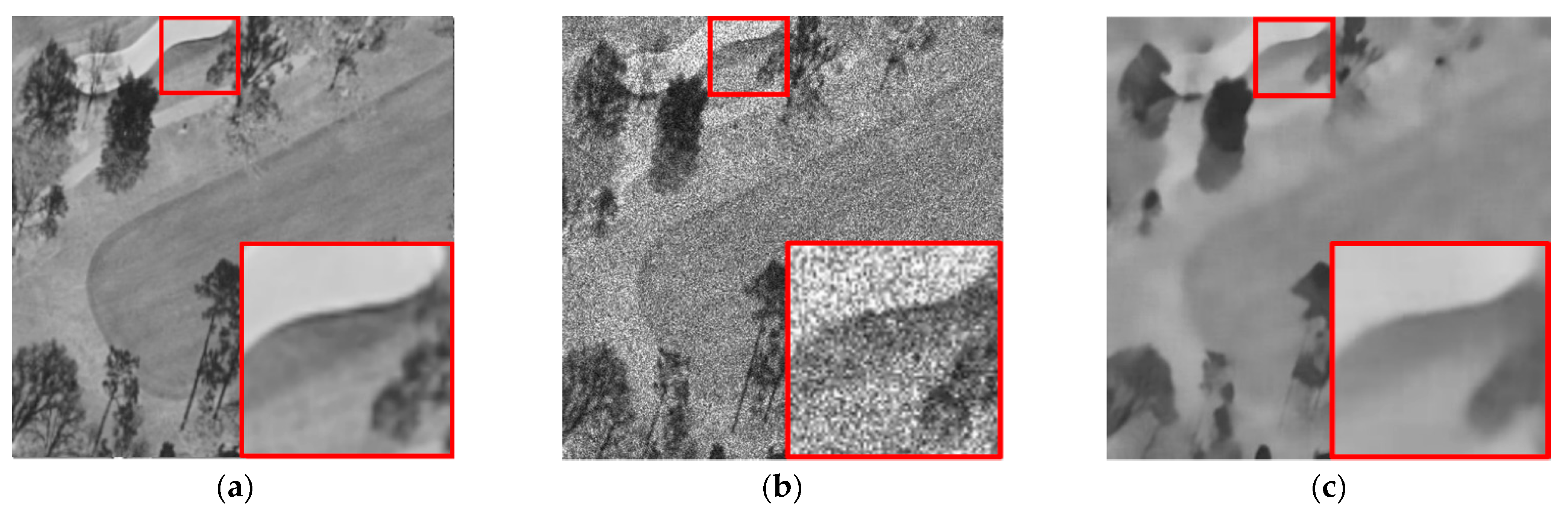
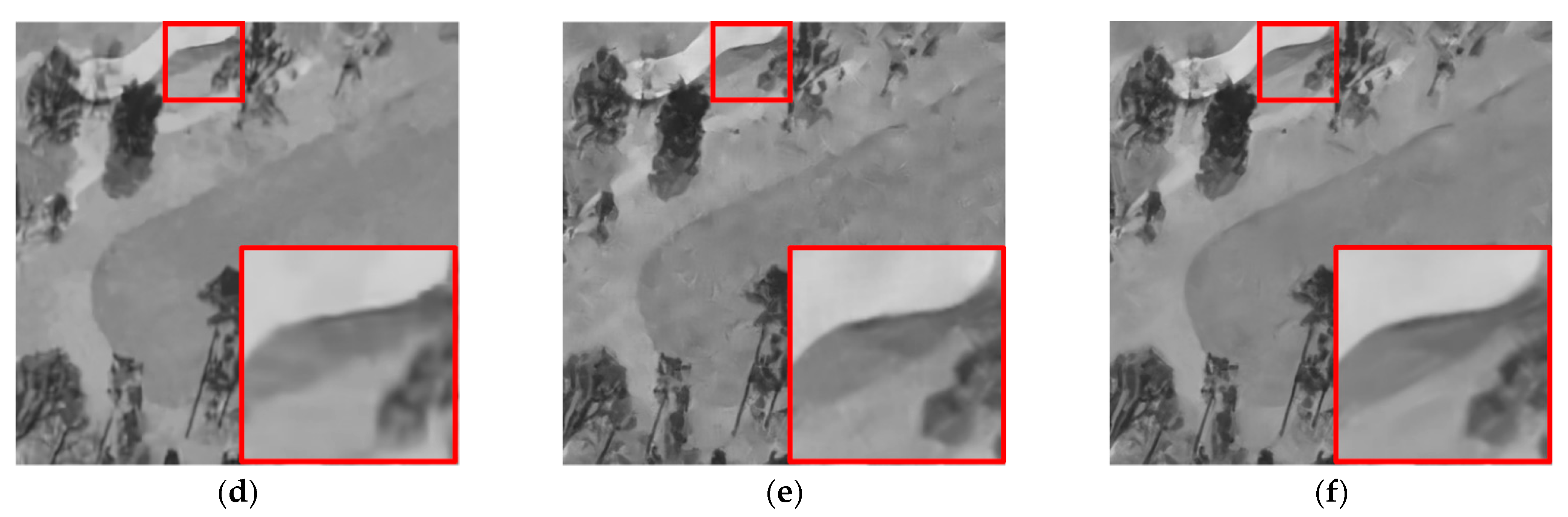
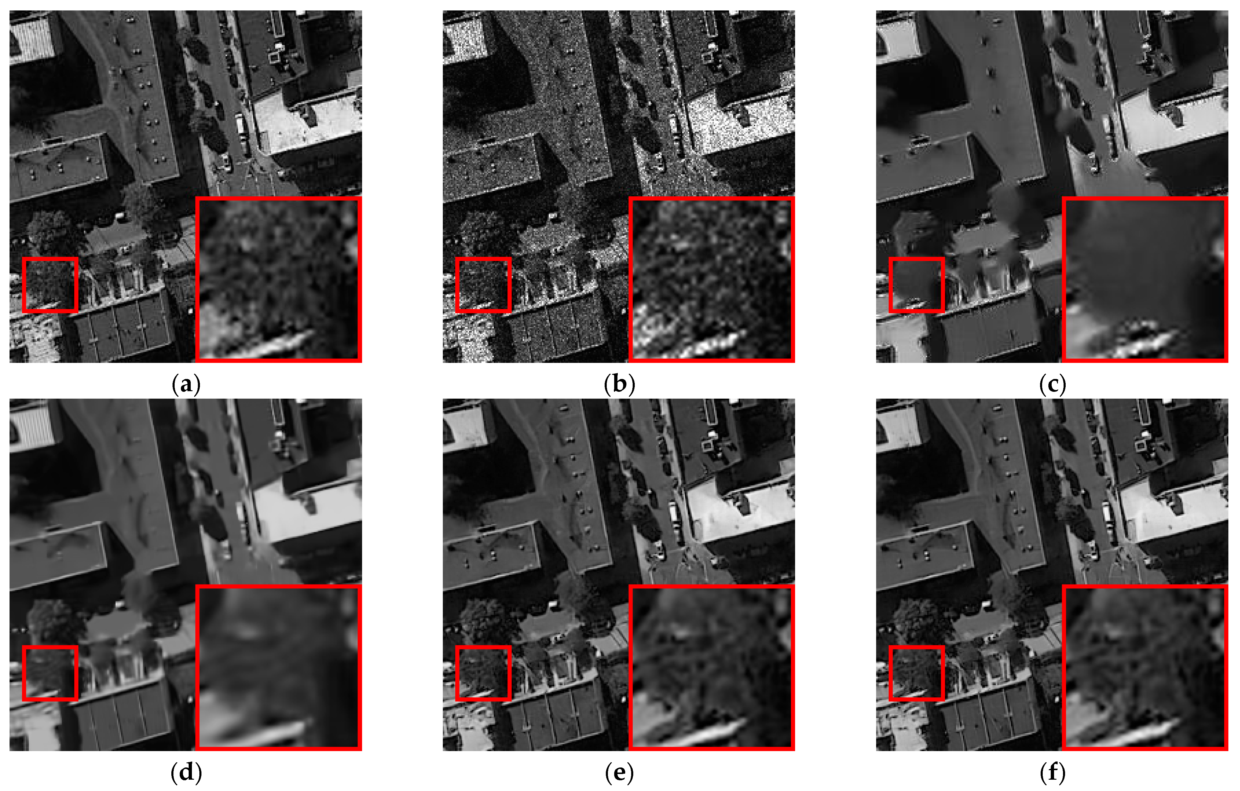
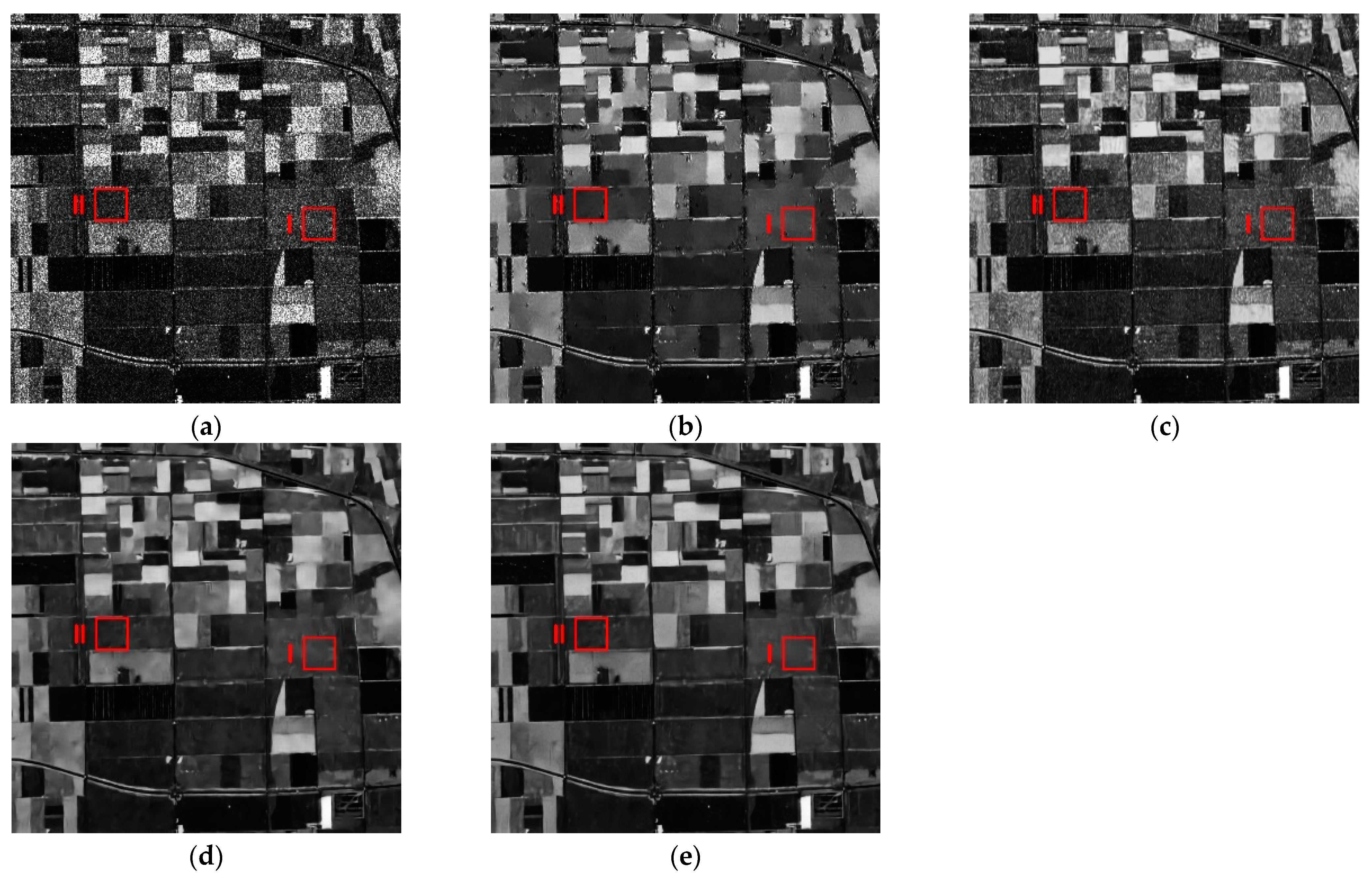
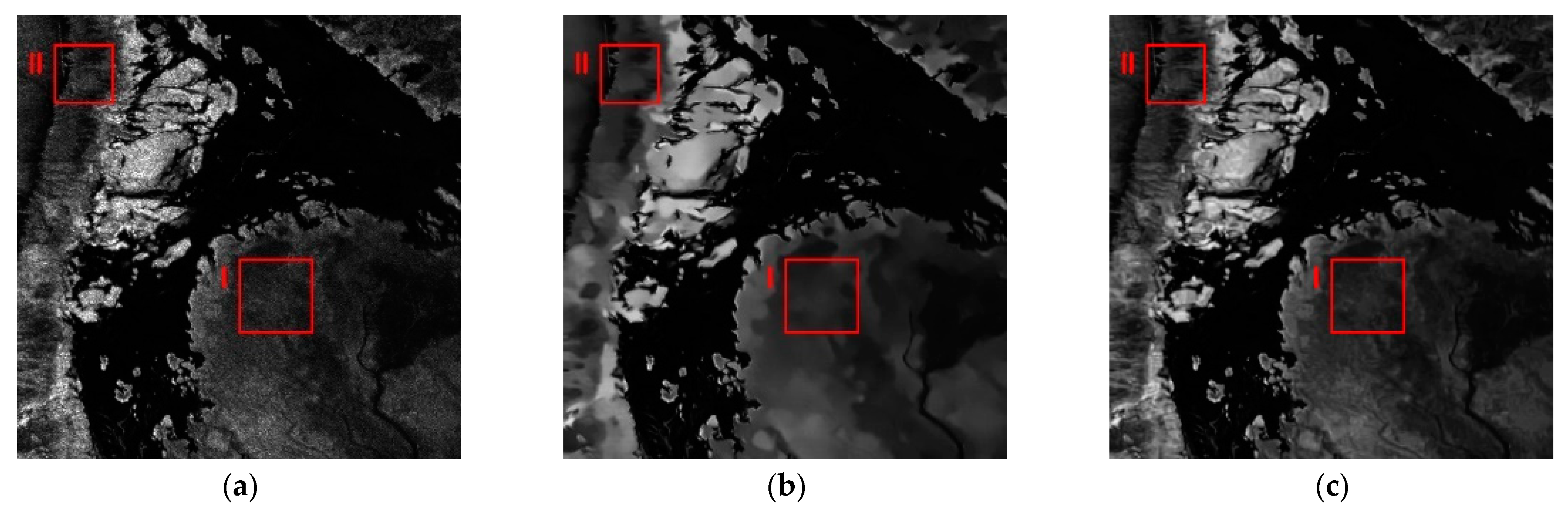
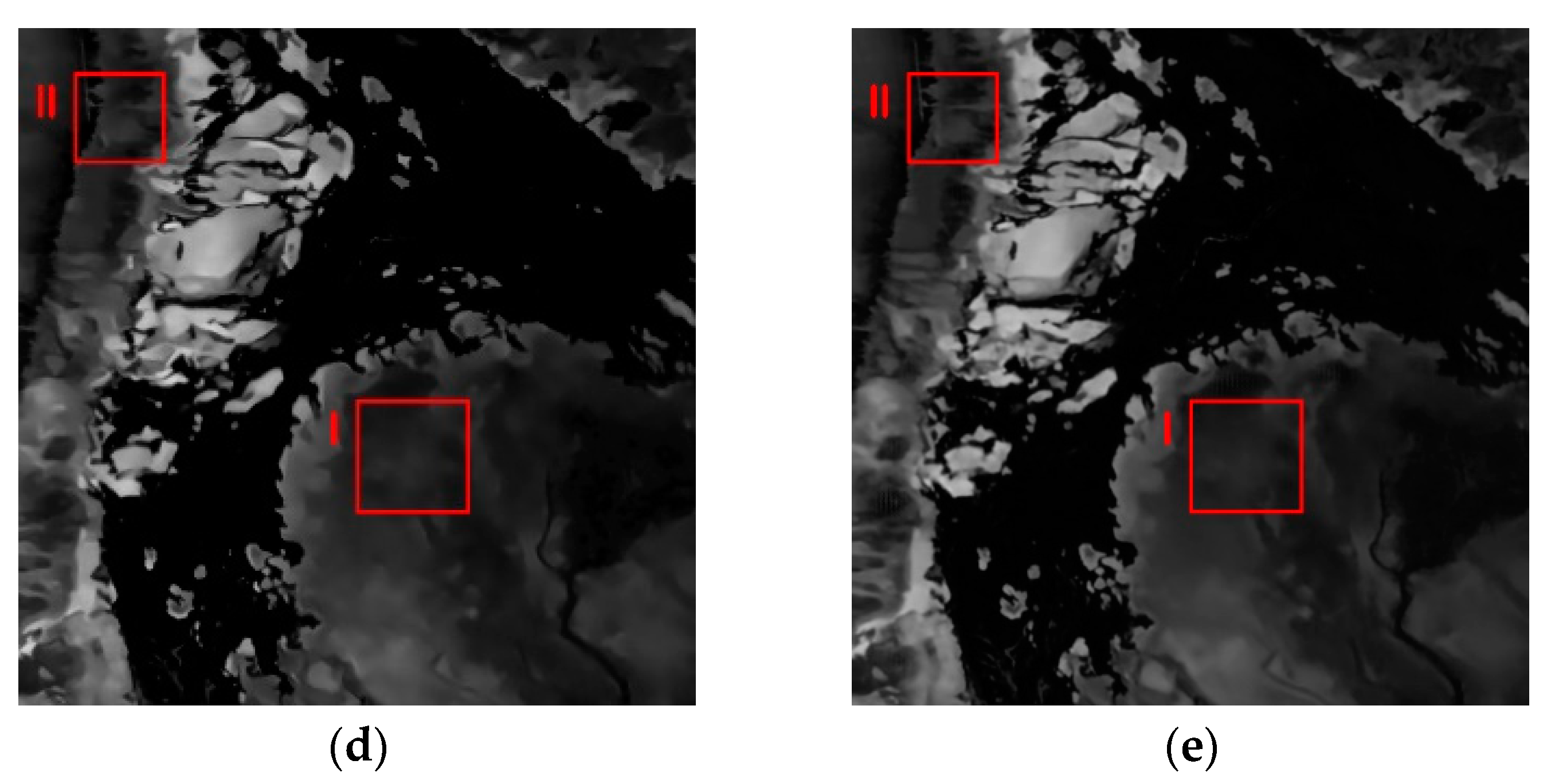
It can be carried out from two aspects—subjective evaluation and objective evaluation—to judge the quality of the denoised images. Subjective evaluation is to observe, analyze, and judge the result of speckle suppression from human vision, which is mainly reflected in the preservation of image texture and detail information. Objective evaluation uses undistorted images as evaluation, and the commonly used indexes are peak signal to noise ratio (PSNR) [61], structural similarity index (SSIM) [62], equivalent numbers of looks (ENL) [63], mean value [64], and standard deviation [65]. In this paper, PSNR and SSIM are used to evaluate the simulated SAR experiment, and ENL is used to evaluate the real SAR image experiment.
(1)
PSNR
PSNR is the most widely used objective evaluation index based on the error between corresponding pixels, which is often defined by mean square error (MSE). MSE is defined as follows:
M S E = 1 m n i = 0 m 1 j = 0 n 1 X i , j Y i , j 2
where X and Y represent two images of m × n sizes, respectively.
The PSNR formula is defined as follows:
P S N R = 20 log 10 M A X M S E
where MAX represents the maximum pixel value of the image. The higher the PSNR value is, the better the effect of noise suppression is.
(2)
SSIM
SSIM mainly measures the similarity between the denoised image and the reference image, which is mainly reflected in brightness, contrast, and structure. The interval range of SSIM value is generally between 0 and 1. The closer it is to 1, the higher the similarity between the two images is, which results in better image processing. The calculation method is as follows:
S S I M m , n = 2 μ m μ n + c 1 2 σ m n + c 2 μ m 2 + μ n 2 + c 1 σ x 2 + σ y 2 + c 2
where m and n are two images, μ m and μ n are the mean values of image m and image n, σ x 2 and σ y 2 are the variances of image m and image n, and σ m n is the covariance. c 1 and c 2 are constants to avoid division by zero.
(3)
ENL
ENL is a generally accepted speckle reduction index in the field of SAR image speckle suppression. It can measure the smoothness of the homogeneous region. The larger the value is, the smoother the region is and the better the noise suppression effect is as well. The formula can be defined as:
E N L = F C μ 2 σ 2
where F C is a constant related to the SAR image format, and if it is a SAR image with intensity format, F C = 1 . If the SAR image is in amplitude format, then F C = 4 / π 1 . μ and σ 2 represent the mean and the variance of the region, respectively.

3. Results

A series of experiments are set to evaluate the performance of the proposed model in Section 3. The despeckled results on synthetic SAR images are shown in this section. Additionally, the despeckling performance with the changing of network parameters numbers is investigated. Finally, the real SAR images are used to test the effectiveness of the proposed method, and the performance evaluated by the ENL is compared with some state-of-the-art methods, including PPB, SAR-BM3D, and ID-CNN. Besides, this section uses forest images to verify the effectiveness of the method. Specially, it is shown that ID-CNN outperforms PPB and SAR-BM3D in ref. [38].

3.1. Performance Analysis of M-xUnit Activation Function

In these experiments, the NWPU-RESISC45 dataset [66] was used for training and testing. In the dataset, 400 images with sizes of 256 × 256 pixels were chosen for training, and 10 images with sizes of 256 × 256 pixels were selected to test. These images cover more than 100 countries and regions all over the world, including developing, transitioning, and highly developed economies. This dataset was also collected by the experts in the field of remote sensing image interpretation from Google Earth (Google Inc.). These training images and test images are shown in Figure 4 and Figure 5, respectively. In order to enhance the training data, these images were scaled in proportion to 1, 0.9, 0.8, and 0.7, and the scaled images were randomly flipped and rotated. The patches with sizes of 40 × 40 were extracted from training images with a step size of 10, and 547,584 patches were obtained. Finally, these patches were synthesized with speckle noise to obtain the synthetic SAR images. Figure 6a shows the process of simulated SAR images. A speckle noise was generated by Equation (2). Then, a multiplicative noise model was established between the noise and the clean image.
The training process of this model took a total of 60 epochs with a mini-batch size of 128. The Adam method [67,68] with the default setting of the gradient descent optimization method was used. The initial learning rate was 0.001 and was multiplied by the decay factor 0.1 after 30 epochs. The proposed method was implemented in Pytorch, and all experiments were tested in the Windows 10 environment with an Intel Core CPU 3.7 GHz and an NVIDIA RTX 2080 GPU.
Inspired by the principle of xUnit [51], the M-xUnit was applied in the SAR image despeckling task. In this paper, ID-CNN [38] was used to test the performance of this spatial learnable activation. The noise estimation part of the network consisted of eight convolutional layers. The main reason for choosing the ID-CNN structure was that the network structure is not affected by some structures such as dilated convolution, skip connections, and densely connected networks. The proposed CNN architecture is shown in Figure 6b, and the detailed configurations of the structure are described in Table 1. Differing from ID-CNN, a series structure with convolution operation, batch normalization (BN), and M-xUnit was employed in L2 to L7.
Figure 7a,b shows the average PSNR results of two different denoisers whose activation functions were M-xUnit and ReLU, respectively. Figure 7a shows the denoising results of ID-CNN with different numbers of M-xUnit. M-xUnit-1 meant that only one layer of “Conv + BN + M-xUnit” was added in the middle of the network, and the total number of network layers was three. Figure 7b presents the denoising results of ID-CNN with regular ReLU activation function; the layer setups were the same as Figure 7a for comparison. We can see that ID-CNN with M-xUnit outperformed the original ID-CNN for all six different layer setups.
To further facilitate the superiority of M-xUnit, we set the number of parameters as abscissa in Figure 7c,d to show the relationship between denoising performance and network complexity. It was found that PSNR and SSIM values obtained by two layers of “Conv + BN + M-xUnit” were equivalent to those obtained by six layers of “Conv + BN + ReLU”, and in the case of three layers, its performance was completely superior to that of ID-CNN. We can also see that the parameters of two layers of “Conv + BN + M-xUnit” were fewer than half of the parameters required by ID-CNN, and the comparison is shown in Table 2.
Comparing the structure of M-xUnit and ReLU in Figure 2, it increased the number of network parameters if the ReLU was merely replaced by the modified xUnit. This meant more memory consumption and running time at the training and the testing stages were required. In [51], compared with ReLU, the xUnit based structure could achieve the same performance with fewer network layers. Finally, fewer network parameters were involved.
To prove that the M-xUnit has better performance on the ID-CNN structure than the original xUnit, a test experiment was conducted in advance. As shown in Table 3, the average PSNR of 10 test images, which are shown in Figure 6, with the speckle noise level of L = 10 for the two structures was compared. It was found that M-xUnit and xUnit activation functions had almost the same performance for the 10 tested images, but the proposed M-xUnit structure was simpler, which meant fewer network training parameters and fewer computational resources were needed for the proposed structure.

3.2. Results on Synthetic SAR Images

To verify the denoising effectiveness with known noise level in SAR image despeckling, three different speckle noise levels of L = 1, 4, and 10 were set up for the test images. In this paper, peak signal to noise ratio (PSNR) and structural similarity (SSIM) were used to evaluate the denoising effectiveness for synthetic SAR images, and the results of synthetic despeckled images are listed in Table 4.
As shown in Table 4, the proposed method obtained the best denoising results compared to the other methods in all the different noisy levels. We found that the proposed method achieved the best denoising results compared to other methods for all the different noisy levels. Figure 8 and Figure 9 show the despeckled results affected by speckle noise level of L = 4. It can be observed that the despeckled results were consistent with the visual results by comparing the zoomed-in patches shown at the lower right corner of these images.

3.3. Results on Real SAR Images

In Section 3.3, the real Flevoland and the Death Valley SAR images were evaluated for the despeckling test by the proposed method and some other state-of-the-art methods, shown in Figure 10 and Figure 11. The Flevoland and the Death Valley SAR images were acquired by the airborne synthetic aperture radar (AIRSAR) and cropped to 600 × 600 pixels as the test SAR image.
It can be observed that the despeckled result by SAR-BM3D still contained residual speckle noise. Moreover, a few texture distortions were generated after the PPB processing. Based on the visual inspection, the ID-CNN performed almost as well as the proposed method for the despeckling. The difference was quite small. Since there were no speckle-free data for the real SAR images, the ENL was employed to measure the performance of different methods. In Figure 10 and Figure 11, the ENL values are estimated from the two homogeneous regions within the red square.
As listed in Table 5 and Table 6, the proposed method attained a better performance in speckle reduction than the other methods.

3.4. Method Validation on Optical Images

From the above subjective analysis, it can be seen that this method was very effective for SAR image speckle suppression. For better analysis and verification, the three tree images were selected from the human vision aspect, which was an optical image taken by a small unmanned aerial vehicle (UAV) produced by China DJI (AIR 2S, DA2SUE1). As shown in Figure 12, they are coniferous forest, broad-leaved forest, and conifer broad-leaved mixed forest.
Most conifers [69] are evergreens, many of which have long and slender leaves with a needlelike appearance, including most of the Taxodiaceae. These leaves are linear, flattened, straight or slightly curved, pectinately arranged, obtusely pointed or shortly mucronate, tapering abruptly towards the articulated junction of the lamina with the decurrent base. The broad-leaved tree [70] (such as maple or oak) can be distinguished from trees bearing needlelike leaves (such as most conifers) by having relatively broad flat leaves and leaf texture, and the most common are oak (sessile and pedunculate) and birch (silver and downy), but ash, sycamore, and beech are also quite common. Under the airborne perspective, coniferous trees are generally darker than broad-leaved trees, with clear tree crown boundaries, but the clarity of coniferous tree leaves is blurred. The main reason is that broad leaf has an obvious texture while conifer does not [71,72,73]. This experiment selected the Metasequoia glyptostroboides forest of Nanjing University of Science and Technology as the coniferous forest image, the broad-leaved trees near the bandstand of Sun Yat-sen Mausoleum as the broad-leaved forest image, and the tree species near Sun Yat-sen Mausoleum Meiling Palace as the conifer broad-leaved mixed forest image, as shown in Figure 12a,d,g, respectively. The tree species in Figure 12d,g included taxodiaceae, pine, plane tree, Cinnamomum camphora, Photinia serrulata, etc.
Visually, due to complications stemming from the original numerous needles interlacing with each other and inadequate characterization based on the limited pixel resolution, the leaves of the coniferous forest after denoising were relatively blurred, each of which were hard to distinguish, as shown in Figure 12c. The leaves of the broad-leaved forest after denoising had a clear boundary because each leaf occupied several pixels, which was conducive to texture rendering and presence in Figure 12f. As can be seen from Figure 12i, after denoising, the leaves of conifers were blurred into blocks (marked with red circles), while those of broad-leaved trees retained obvious texture (marked with red rectangles), and the clarity of broad-leaved trees was higher than that of conifers.
For better analysis, the two relevant indices (i.e., PSNR and SSIM) are given in Table 7. The higher the PSNR value was, the better the effect of noise suppression was.
The coniferous forest image had the lowest value (22.75 dB) of PSNR, while the broad-leaved forest image had the highest value (24.94 dB) of PSNR, which shows that the denoising effect of the broad-leaved forest was better than that of the coniferous forest. The closer SSIM was to one, the higher the similarity was between the two images, which resulted in better kept image details. It can be seen that the SSIM of the coniferous forest was 0.778 dB, and that of the broad-leaved forest was 0.806, from which we can infer that the image details of the broad-leaved forest were better preserved after denoising. Because the coniferous and the broad-leaved tree crowns were staggered, the two indices of the conifer broad-leaved mixed forest (PSNR 23.46 dB and SSIM 0.785) were lower than those of the broad-leaved forest and higher than those of the coniferous forest. Figure 12i shows a coniferous trees crown with an ambiguous upper appearance due to information loss caused by insensitivity of activatable functions for minute details (red circle marks) and broad-leaved trees with clear texture (red rectangle marks) because the activatable function had higher recognition of texture.
A well-denoised image can be obtained by our method, which is helpful to identify conifers and broad-leaved trees from the conifer broad-leaved mixed forest. It can also be concluded that our method is effective for multiplicative noise.

4. Discussion

The reason the convolutional neutral network method was used to suppress the speckle was that the traditional algorithm could improve the performance of noise suppression by introducing a new algorithm structure. However, detailed information could be still missing. The speckle suppression performance would be degraded if more details were to be retained. Therefore, traditional algorithms should seek the maximum balance between speckle suppression performance and information preservation. The speckle suppression itself is to solve the mapping problem from the observed image to the noise-free image. By virtue of its powerful feature extraction ability, convolutional neural networks achieve end-to-end mapping and good results in speckle suppression and information preservation. Convolutional neural networks are widely used in SAR image speckle suppression because of the advantages that this traditional algorithm does not have. Deep convolution neural networks achieve unprecedented performance in many low-level vision tasks, such as super-resolution reconstruction, image denoising, target detection, and recognition. However, the most advanced result is usually to design a very deep network with tens of millions of network parameters, which greatly limits the implementation of the algorithm on resource-limited platforms. Therefore, it is a challenge to run network models using low power and resource-limited platforms.
At present, scholars have done a great deal of research in reducing model parameters. One option is to improve convolution operation, such as 1 × 1 convolution, ACNet, and MobileNet. The second is to improve the activation function, such as Leaky ReLU, PReLU, DyReLU, and xUnit. Among them, PReLU, DyReLU, and xUnit are activation functions with learnable parameters. Their essence is to add learnable parameters to the activation function of the convolution layer, and their performance is much better than common ReLU functions. Although the number of additional parameters will be increased, this kind of function is characterized by its ability to achieve the same performance as the original network model with fewer network layers, thereby further reducing the parameters of these models without degrading the performance. Although convolutional neural networks have achieved very good results in SAR image speckle suppression, the structure has gradually changed from simple to complex with depth gradually changing from shallow to deep, resulting in an increasing complexity and thus requiring a large number of computing resources. This paper further improved the performance by introducing a learnable activation function at the cost of a small number of parameters.
We mainly introduced parameters that could be trained and learned with the network in the process of nonlinear operation, that is, spatial processing was introduced in the process of nonlinear operation, which constituted the structure of the algorithm. As shown in Figure 2c, the constructed weight mapping achieved nonlinear operation through a ReLU activation function and then successively deeply convolved with the Tanh function, and, finally, the weight range was mapped between [−1, 1]. Tanh was introduced to solve the problem that the output of the ReLU method was not zero-centered, making up for the defect that the element value was zero by ReLU when it was less than or equal to zero so as to prevent some cells from being activated. Compared with other algorithms, this algorithm is easier to implement, which makes it easy for readers to analyze and operate. In Section 3, 10 test images were used to evaluate the proposed method and ID-CNN by gradually reducing “Conv + BN + M-xUnit” and “Conv + BN + ReLU” blocks, as shown in Figure 7a,b. The training configuration was the same in both networks, and the network configuration is displayed in Table 1. The performances of the modified networks based on xUnit and ReLU with respect to number of parameters were compared, as demonstrated in Figure 7c,d. As can be seen from the figure, the proposed method achieved higher PSNR and SSIM with the same number of parameters. Alternatively, the modified xUnit-based network achieved the same PSNR and SSIM with significantly fewer parameters, suggesting, in the case of training models with large parameters, the “Conv + BN + ReLU” blocks can be replaced with fewer “Conv + BN + M-xUnit” blocks. Finally, this algorithm required little computational memory and time for speckling.
Based on the above analysis and discussion, the whole experiment achieved the expected effect, which exceeded the traditional methods.

5. Conclusions

A SAR image despeckling method using a CNN platform with a new learnable spatial activation function, M-xUnit, was proposed in this paper. Compared with the most advanced speckle processing methods, fewer network parameters were required for training without degrading performance. In addition to designing complex network structures for better despeckled results, improving the activation function is also a preferred choice for SAR image speckle suppression tasks. A total of 400 training images and 10 test images were used to illustrate the performance of the proposed method, and its effectiveness was verified by using real SAR images and forest optical images. Despeckling experiments on both synthetic and real SAR images indicate that the proposed method outperforms some state-of-the-art despeckling methods. We also applied the proposed method to forest optical images and achieved good results. It was also found that there was a large difference in the despeckling effect between coniferous forest and broad-leaved forest and thus concluded that the despeckling effect of the broad-leaved forest was better than that of the coniferous forest.
In future work, the method proposed in this paper will be extended by adding other algorithms so as to perform better and be applicable to a wider range of fields.

Author Contributions

Study design and writing, H.W. and Z.D.; methodology, S.T.; project administration, S.T. and H.W.; conceptualization, S.S. and Z.D.; software, S.S. and X.L.; data curation, X.Y.; investigation, D.Z. All authors have read and agreed to the published version of the manuscript.

Funding

This research was funded by the National Natural Science Foundation of China, grant number 61701240.

Institutional Review Board Statement

Not applicable.

Informed Consent Statement

Not applicable.

Data Availability Statement

The NWPU-RESISC45 dataset presented in this study are openly available in reference number [66]. Publicly available forest images were analyzed in this study. This data can be found here: https://pan.baidu.com/s/1SDGmDxxHN_Fxc5PZIigqjg (senn) (accessed on 1 July 2021).

Acknowledgments

The authors would like to thank the National Natural Science Foundation of China and Shifei Tao of Nanjing University of Science and Technology in China for financially supporting this research.

Conflicts of Interest

The authors declare no conflict of interest.

References

  1. Xiaoli, Y.; Hoff, L.E.; Reed, I.S.; Chen, A.M.; Stotts, L.B. Automatic Target Detection and Recognition in Multiband Imagery: A Unified ML Detection and Estimation Approach. IEEE Trans. Image Process. 1997, 6, 143–156. [Google Scholar] [CrossRef]
  2. Chen, X.; Chen, B.; Guan, J.; Huang, Y.; He, Y. Space-Range-Doppler Focus-Based Low-observable Moving Target Detection Using Frequency Diverse Array MIMO Radar. IEEE Access 2018, 6, 43892–43904. [Google Scholar] [CrossRef]
  3. Jafarian, J.H.; Shaer, E.A.; Duan, Q. An Effective Address Mutation Approach for Disrupting Reconnaissance Attacks. IEEE Trans. Inf. Forensics Secur. 2015, 10, 2562–2577. [Google Scholar] [CrossRef]
  4. Wan, P.; Hao, B.; Li, Z.; Ma, X.; Zhao, Y. Accurate Estimation the Scanning Cycle of the Reconnaissance Radar Based on a Single Unmanned Aerial Vehicle. IEEE Access 2017, 5, 22871–22879. [Google Scholar] [CrossRef]
  5. Davarian, F.; Shambayati, S.; Slobin, S. Deep Space Ka-band Link Management and Mars Reconnaissance Orbiter: Long-term Weather Statistics Versus Forecasting. Proc. IEEE 2004, 92, 1879–1894. [Google Scholar] [CrossRef]
  6. Zurowietz, M.; Nattkemper, T.W. Unsupervised Knowledge Transfer for Object Detection in Marine Environmental Monitoring and Exploration. IEEE Access 2020, 8, 143558–143568. [Google Scholar] [CrossRef]
  7. Meskin, N.; Khorasani, K.; Rabbath, C.A. A Hybrid Fault Detection and Isolation Strategy for a Network of Unmanned Vehicles in Presence of Large Environmental Disturbances. IEEE Trans. Control Syst. Technol. 2010, 18, 1422–1429. [Google Scholar] [CrossRef]
  8. Huang, D.; Guo, X.; Zhang, Z.; Yu, W.; Truong, T. Full-Aperture Azimuth Spatial-Variant Autofocus Based on Contrast Maximization for Highly Squinted Synthetic Aperture Radar. IEEE Trans. Geosci. Remote Sens. 2020, 58, 330–347. [Google Scholar] [CrossRef]
  9. Zeng, T.; Wei, Y.; Ding, Z.; Chen, X.; Wang, Y.; Fan, Y.; Long, T. Parametric Image Reconstruction for Edge Recovery from Synthetic Aperture Radar Echoes. IEEE Trans. Geosci. Remote Sens. 2021, 59, 2155–2173. [Google Scholar] [CrossRef]
  10. Schartel, M.; Burr, R.; Mayer, W.; Waldschmidt, C. Airborne Tripwire Detection Using a Synthetic Aperture Radar. IEEE Geosci. Remote Sens. Lett. 2020, 17, 262–266. [Google Scholar] [CrossRef]
  11. Moccia, A.; Chiacchio, A.; Capone, A. Spaceborne bistatic Synthetic Aperture Radar for remote sensing applications. Int. J. Remote Sens. 2000, 21, 3395–3414. [Google Scholar] [CrossRef]
  12. Chen, S.; Li, X.; Chi, S.; Li, Z.; Yuxing, M. Ship Target Discrimination in SAR Images Based on BOW Model with Multiple Features and Spatial Pyramid Matching. IEEE Access 2020, 8, 166071–166082. [Google Scholar] [CrossRef]
  13. Han, L.; Ran, D.; Ye, W.; Yang, W.; Wu, X. Multi-Size Convolution and Learning Deep Network for SAR Ship Detection from Scratch. IEEE Access 2020, 8, 158996–159016. [Google Scholar] [CrossRef]
  14. Ulaby, F.T.; Dobson, M.C. Handbook of Radar Scattering Statistics for Terrain; Artech House: Norwood, MA, USA, 1989. [Google Scholar]
  15. Thompson, P.; Wahl, D.E.; Eichel, H.P.; Ghiglia, D.C.; Jakowatz, C.V. Spotlight-Mode Synthetic Aperture Radar: A Signal Processing Approach; Kluwer: Norwell, MA, USA, 1996. [Google Scholar]
  16. Xu, J.; Li, G.; Peng, Y.; Xia, X.; Wang, Y. Parametric Velocity Synthetic Aperture Radar: Multilook Processing and Its Applications. IEEE Trans. Geosci. Remote Sens. 2008, 46, 3488–3502. [Google Scholar] [CrossRef]
  17. Zhu, S.; Liao, G.; Tao, H.; Qu, Y.; Yang, Z. Ground Moving Target Detection and Velocity Estimation Based on Spatial Multilook Processing for Multichannel Airborne SAR. IEEE Trans. Aerosp. Electron. Syst. 2013, 49, 1322–1337. [Google Scholar] [CrossRef]
  18. Raj, R.G.; Rodenbeck, C.T.; Lipps, R.D.; Jansen, R.W.; Ainsworth, T.L. A Multilook Processing Approach to 3-D ISAR Imaging Using Phased Arrays. IEEE Geosci. Remote Sens. Lett. 2018, 15, 1412–1416. [Google Scholar] [CrossRef]
  19. Wu, H.; Xu, H.; Wang, P.; Yang, B.; Li, C. Denoising Method Based on Intrascale Correlation in Nonsubsampled Contourlet Transform for Synthetic Aperture Radar Images. J. Appl. Remote Sens. 2019, 13, 046503. [Google Scholar] [CrossRef]
  20. Kuan, D.T.; Sawchuk, A.A.; Strand, T.C.; Chavel, P. Adaptive Noise Smoothing Filter for Images with Signal-dependent Noise. IEEE Trans. Pattern Anal. Mach. Intell. 1985, 7, 165–177. [Google Scholar] [CrossRef] [PubMed]
  21. Schaller, S.; Wildberger, J.E.; Raupach, R.; Niethammer, M.; Klingenbeck-Regn, K.; Flohr, T. Spatial Domain Filtering for Fast Modification of the Tradeoff Between Image Sharpness and Pixel Noise in Computed Tomography. IEEE Trans. Med. Imaging 2003, 22, 846–853. [Google Scholar] [CrossRef]
  22. Chaudhuri, B.B. A Note on Fast Algorithms for Spatial Domain Techniques in Image Processing. IEEE Trans. Syst. 1983, 13, 1166–1169. [Google Scholar] [CrossRef]
  23. Mahdianpari, M.; Salehi, B.; Mohammadimanesh, F. The Effect of PolSAR Image Despeckling on Wetland Classification: Introducing a New Adaptive Method. J. Appl. Remote Sens. 2017, 43, 485–503. [Google Scholar]
  24. Wang, C.Y.; Hu, Y.K.; Wu, S.X. Shearlet Domain SAR Image Denoising Method Based on Bayesian Model. Syst. Eng. Electron. 2017, 39, 1250–1255. [Google Scholar]
  25. Zada, S.; Tounsi, Y.; Kumar, M.; Mendoza-Santoyo, F.; Nassim, A. Contribution Study of Monogenic Wavelets Transform to Reduce Speckle Noise in Digital Speckle Pattern Interferometry. Opt. Eng. 2019, 58, 034109. [Google Scholar] [CrossRef]
  26. Celik, T.; Tjahjadi, T. Image Resolution Enhancement Using Dual-Tree Complex Wavelet Transform. IEEE Geosci. Remote Sens. Lett. 2010, 7, 554–557. [Google Scholar] [CrossRef] [Green Version]
  27. Shen, F.; Wang, Y.; Liu, C. Synthetic Aperture Radar Image Change Detection Based on Kalman Filter and Nonlocal Means Filter in the Nonsubsampled Shearlet Transform Domain. J. Appl. Remote Sens. 2020, 14, 016517. [Google Scholar] [CrossRef]
  28. Deledalle, C.; Denis, L.; Tupin, F. Iterative Weighted Maximum Likelihood Denoising with Probabilistic Patch-based Weights. IEEE Trans. Image Process. 2009, 18, 2661–2672. [Google Scholar] [CrossRef] [PubMed] [Green Version]
  29. Parrilli, S.; Poderico, M.; Angelino, C.V.; Verdoliva, L. A Nonlocal SAR Image Denoising Algorithm Based on LLMMSE Wavelet Shrinkage. IEEE Trans. Geosci. Remote Sens. 2012, 50, 606–616. [Google Scholar] [CrossRef]
  30. Xie, Z.; Liu, L.; Yang, C. A Probabilistic Model-Based Method with Nonlocal Filtering for Robust Magnetic Resonance Imaging Reconstruction. IEEE Access 2020, 8, 82347–82363. [Google Scholar] [CrossRef]
  31. Zhao, Y.; Liu, J.G.; Zhang, B.; Hong, W.; Wu, Y. Adaptive Total Variation Regularization Based SAR Image Despeckling and Despeckling Evaluation Index. IEEE Trans. Geosci. Remote Sens. 2015, 53, 2765–2774. [Google Scholar] [CrossRef] [Green Version]
  32. Feng, W.; Lei, H.; Gao, Y. Speckle Reduction Via Higher Order Total Variation Approach. IEEE Trans. Image Process. 2014, 23, 1831–1843. [Google Scholar] [CrossRef]
  33. Aggarwal, H.K.; Majumdar, A. Hyperspectral Image Denoising Using Spatio-Spectral Total Variation. IEEE Geosci. Remote Sens. Lett. 2016, 13, 442–446. [Google Scholar] [CrossRef]
  34. Chang, Y.; Yan, L.; Fang, H.; Luo, C. Anisotropic Spectral-Spatial Total Variation Model for Multispectral Remote Sensing Image Destriping. IEEE Trans. Image Process. 2015, 24, 1852–1866. [Google Scholar] [CrossRef]
  35. Zhang, K.; Zuo, W.; Chen, Y.; Meng, D.; Zhang, L. Beyond a Gaussian Denoiser: Residual Learning of Deep CNN for Image Denoising. IEEE Trans. Image Process. 2017, 26, 3142–3155. [Google Scholar] [CrossRef] [PubMed] [Green Version]
  36. Chierchia, G.; Cozzolino, D.; Poggi, G.; Verdoliva, L. SAR Image Despeckling through Convolutional Neural Networks. In Proceedings of the IEEE International Geoscience and Remote Sensing Symposium (IGARSS), Fort Worth, TX, USA, 23–28 July 2017; pp. 5438–5441. [Google Scholar]
  37. He, K.; Zhang, X.; Ren, S.; Sun, J. Deep Residual Learning for Image Recognition. In Proceedings of the IEEE Conference on Computer Vision and Pattern Recognition (CVPR), Las Vegas, NV, USA, 27–30 June 2016; pp. 770–778. [Google Scholar]
  38. Wang, P.; Zhang, H.; Patel, V.M. SAR Image Despeckling Using a Convolutional Neural Network. IEEE Signal Process Lett. 2017, 24, 1763–1767. [Google Scholar] [CrossRef] [Green Version]
  39. Zhang, Q.; Yuan, Q.; Li, J.; Yang, Z.; Ma, X. Learning A Dilated Residual Network for SAR Image Despeckling. Remote Sens. 2018, 10, 196. [Google Scholar] [CrossRef] [Green Version]
  40. Zhang, W.; Quan, H.; Gandhi, O.; Rajagopal, R.; Tan, C.W.; Srinivasan, D. Improving Probabilistic Load Forecasting Using Quantile Regression NN with Skip Connections. IEEE Trans. Smart Grid 2020, 11, 5442–5450. [Google Scholar] [CrossRef]
  41. Zhang, Z.; Wang, X.; Jung, C. DCSR: Dilated Convolutions for Single Image Super-Resolution. IEEE Trans. Image Process. 2018, 28, 1625–1635. [Google Scholar] [CrossRef]
  42. Gui, Y.; Xue, L.; Li, X. SAR Image Despeckling Using a Dilated Densely Connected Network. Remote Sens. Lett. 2018, 9, 857–866. [Google Scholar] [CrossRef]
  43. Huang, G.; Liu, Z.; Maaten, L.V.D.; Weinberger, K.Q. Densely Connected Convolutional Networks. In Proceedings of the IEEE Conference on Computer Vision and Pattern Recognition (CVPR), Honolulu, HI, USA, 21–26 July 2017; pp. 2261–2269. [Google Scholar]
  44. Lattari, F.; Leon, B.G.; Asaro, F.; Rucci, A.; Prati, C.; Matteucci, M. Deep Learning for SAR Image Despeckling. Remote Sens. 2017, 11, 1532. [Google Scholar] [CrossRef] [Green Version]
  45. Cozzolino, D.; Verdoliva, L.; Scarpa, G.; Poggi, G. Nonlocal CNN SAR Image Despeckling. Remote Sens. 2020, 12, 1006. [Google Scholar] [CrossRef] [Green Version]
  46. He, L.; Greenshields, I.R. A Nonlocal Maximum Likelihood Estimation Method for Rician Noise Reduction in MR Images. IEEE Trans. Med. Imaging 2009, 28, 165–172. [Google Scholar]
  47. Cozzolino, D.; Verdoliva, L.; Scarpa, G.; Poggi, G. Nonlocal Sar Image Despeckling by Convolutional Neural Networks. In Proceedings of the 2019 IEEE International Geoscience and Remote Sensing Symposium, Yokohama, Japan, 28 July–2 August 2019; pp. 5117–5120. [Google Scholar]
  48. Liu, S.; Liu, T.; Gao, L.; Li, H.; Hu, Q.; Zhao, J.; Wang, C. Convolutional neural network and guided filtering for SAR image denoising. Remote Sens. 2019, 11, 702. [Google Scholar] [CrossRef] [Green Version]
  49. Li, S.; Kang, X.; Hu, J. Image Fusion with Guided Filtering. IEEE Trans. Image Process 2013, 22, 2864–2875. [Google Scholar] [PubMed]
  50. Xiang, L.; Zhao, Y.; Dai, G.; Gou, R.; Zhang, H.; Shi, J. The Study of Chinese Calligraphy Font Style Based on Edge-Guided Filter and Convolutional Neural Network. In Proceedings of the 2020 IEEE 5th International Conference on Signal and Image Processing (ICSIP), Nanjing, China, 23–25 October 2020; pp. 883–887. [Google Scholar]
  51. Sobel, M.; Groll, P.A. Group Testing to Eliminate Efficiently All Defectives in A Binomial Sample. Bell Syst. Tech. J. 1959, 38, 1179–1252. [Google Scholar] [CrossRef]
  52. Tsai, C.; Chih, Y.; Wong, W.H.; Lee, C. A Hardware-Efficient Sigmoid Function with Adjustable Precision for a Neural Network System. IEEE Trans. Circuits Syst. II Express Briefs 2015, 62, 1073–1077. [Google Scholar] [CrossRef]
  53. Zhang, S.; Gao, H.; Song, Y. A New Fault-Location Algorithm for Extra-High-Voltage Mixed Lines Based on Phase Characteristics of the Hyperbolic Tangent Function. IEEE Trans. Power Deliv. 2016, 31, 1203–1212. [Google Scholar] [CrossRef]
  54. Wang, D.; Zeng, J.; Lin, S.B. Random Sketching for Neural Networks with ReLU. IEEE Trans. Neural Netw. Learn. Syst. 2021, 32, 748–762. [Google Scholar] [CrossRef] [PubMed]
  55. Chen, Z.; Deng, L.; Li, G.; Sun, J.; Hu, X.; Liang, L.; Ding, Y.; Xie, Y. Effective and Efficient Batch Normalization Using a Few Uncorrelated Data for Statistics Estimation. IEEE Trans. Neural Netw. Learn. Syst. 2021, 32, 348–362. [Google Scholar] [CrossRef]
  56. Lim, B.; Son, S.; Kim, H.; Nah, S.; Lee, K.M. Enhanced Deep Residual Networks for Single Image Super-Resolution. In Proceedings of the IEEE Conference on Computer Vision and Pattern Recognition Workshops (CVPRW), Honolulu, HI, USA, 21–26 July 2017; pp. 1132–1140. [Google Scholar]
  57. Howard, A.G.; Zhu, M.; Chen, B.; Kalenichenko, D.; Wang, W.; Weyand, T.; Andreetto, M.; Adam, H. MobileNets: Efficient Convolutional Neural Networks for Mobile Vision Applications. arXiv 2017, arXiv:1704.04861. [Google Scholar]
  58. Chollet, F. Xception: Deep Learning with Depthwise Separable Convolution. In Proceedings of the 2017 IEEE Conference on Computer Vision and Pattern Recognition (CVPR), Honolulu, HI, USA, 21–26 July 2017; pp. 1800–1807. [Google Scholar]
  59. Chen, X.; Jiang, K.; Zhu, Y.; Wang, X.; Yun, T. Individual Tree Crown Segmentation Directly from UAV-Borne LiDAR Data Using the PointNet of Deep Learning. Remote Sens. 2021, 12, 131. [Google Scholar]
  60. Wang, J.; Chen, X.; Cao, L.; An, F.; Chen, B.; Xue, L.; Yun, T. Individual Rubber Tree Segmentation Based on Ground-Based LiDAR Data and Faster R-CNN of Deep Learning. Forests 2019, 10, 793. [Google Scholar] [CrossRef] [Green Version]
  61. Pendock, G.J.; Sampson, D.D. Signal-to-noise Ratio of Modulated Sources of ASE Transmitted over Dispersive Fiber. IEEE Photonics Technol. Lett. 1997, 9, 1002–1004. [Google Scholar] [CrossRef]
  62. Chai, L.; Sheng, Y. Optimal Design of Multichannel Equalizers for the Structural Similarity Index. IEEE Trans. Image Process. 2014, 23, 5626–5637. [Google Scholar] [CrossRef] [PubMed]
  63. Tao, L.; Gui, C.H.; Min, X.Z.; Jun, G. Texture-Invariant Estimation of Equivalent Number of Looks Based on Trace Moments in Polarimetric Radar Imagery. IEEE Geosci. Remote Sens. Lett. 2014, 11, 1129–1133. [Google Scholar] [CrossRef]
  64. Goumeidane, A.B.; Nacereddine, N. Statistical and Spatial Information Association for Clusters Number and Mean Values Estimation in Image Segmentation. In Proceedings of the 2020 IEEE 4th International Conference on Image Processing, Applications and Systems (IPAS), Genova, Italy, 9–11 December 2020; pp. 206–211. [Google Scholar]
  65. Huo, Z.; Du, G.; Luo, F.; Qiao, Y.; Luo, J. D-MSCD: Mean-Standard Deviation Curve Descriptor Based on Deep Learning. IEEE Access 2020, 8, 204509–204517. [Google Scholar] [CrossRef]
  66. Cheng, G.; Han, J.; Lu, X. Remote Sensing Image Scene Classification: Benchmark and State of the Art. Proc. IEEE 2017, 105, 1865–1883. [Google Scholar] [CrossRef] [Green Version]
  67. Matsumura, S.; Nakashima, T. Incremental Learning for SIRMs Fuzzy Systems by Adam Method. In Proceedings of the 2017 Joint 17th World Congress of International Fuzzy Systems Association and 9th International Conference on Soft Computing and Intelligent Systems (IFSA-SCIS), Otsu, Japan, 27–30 June 2017; pp. 1–4. [Google Scholar]
  68. Kingma, D.; Ba, J. Adam: A Method for Stochastic Optimization. Comput. Sci. 2014, 9, 1–15. [Google Scholar]
  69. Neale, D.B.; Wheeler, N.C. The Conifers. In The Conifers: Genomes, Variation and Evolution; Springer: Cham, Switzerland, 2019. [Google Scholar]
  70. Lin, H.; Peng, H. Machine Recognition for Broad-Leaved Trees Based on Synthetic Features of Leaves Using Probabilistic Neural Network. In Proceedings of the 2008 International Conference on Computer Science and Software Engineering, Wuhan, China, 12–14 December 2008; pp. 871–877. [Google Scholar]
  71. Hossein, T.; Reik, L.; Andreas, H.; Michael, E.S.; Felix, M. Tree species classification in a temperate mixed forest using a combination of imaging spectroscopy and airborne laser scanning. Agric. For. Meteorol. 2019, 279, 107744. [Google Scholar]
  72. Yun, T.; Jiang, K.; Li, G.; Eichhorn, M.P.; Cao, L. Individual tree crown segmentation from airborne LiDAR data using a novel Gaussian filter and energy function minimization-based approach. Remote. Sens. Environ. 2021, 256, 112307. [Google Scholar] [CrossRef]
  73. Waser, L.; Ginzler, C.; Rehush, N. Wall-to-Wall Tree Type Mapping from Countrywide Airborne Remote Sensing Surveys. Remote Sens. 2017, 9, 766. [Google Scholar] [CrossRef] [Green Version]
Figure 1. Four kinds of activation function curves: (a) Sigmoid, (b) Tanh, (c) ReLU, (d) ReLU after derivation.
Remotesensing 13 03444 g001
Figure 2. Three activation blocks: (a) the ReLU after derivation, (b) the structure of xUnit, (c) the modified xUnit.
Remotesensing 13 03444 g002
Figure 3. The difference between two convolution operations: (a) ordinary convolution operation, (b) deep convolution operation.
Remotesensing 13 03444 g003
Figure 4. In total, 18 kinds of images from the NWPU-RESISC45 dataset in different situations were selected as training sets, including farmland, sparse residential, baseball diamond, beach, buildings, chaparral, dense residential, storage tanks, freeway, etc.
Remotesensing 13 03444 g004aRemotesensing 13 03444 g004b
Figure 5. The 10 testing images marked in order from (a) to (j). (a,b) are golf course, (c,d) are basketball court, (e,f) are beach, (g,h) are bridge, (i,j) are medium residential.
Remotesensing 13 03444 g005
Figure 6. The process of the proposed method: (a) the process of simulated SAR image, (b) the proposed CNN architecture for SAR image despeckling.
Remotesensing 13 03444 g006
Figure 7. The performance analysis: (a) simulation curves of different “Conv + BN + M-xUnit” layers when L = 10, (b) simulation curves of different “Conv + BN + ReLU” layers when L = 10, (c) the comparison of PSNR between M-xUnit and ReLU, (d) the comparison of SSIM between M-xUnit and ReLU.
Remotesensing 13 03444 g007
Figure 8. Filtered images of different methods for golf course test image contaminated by four-look speckle. (a) Original image, (b) noisy image, (c) PPB, (d) SAR-BM3D, (e) ID-CNN, (f) proposed.
Remotesensing 13 03444 g008aRemotesensing 13 03444 g008b
Figure 9. Filtered images of different methods for medium residential test image contaminated by four-look speckle. (a) Original image, (b) noisy image, (c) PPB, (d) SAR-BM3D, (e) ID-CNN, (f) proposed.
Remotesensing 13 03444 g009
Figure 10. Despeckle results of different methods for the Flevoland SAR image: (a) original; (b) PPB; (c) SAR-BM3D; (d) ID-CNN; (e) proposed.
Remotesensing 13 03444 g010
Figure 11. Despeckle results of different methods for the Death Valley SAR image: (a) original; (b) PPB; (c) SAR-BM3D; (d) ID-CNN; (e) proposed.
Remotesensing 13 03444 g011aRemotesensing 13 03444 g011b
Figure 12. Three forest aerial images were chosen as the experimental objects to analyze the performance of our deep learning method. (a) The original image of the pure coniferous forest comprising Metasequoia glyptostroboides in Nanjing University of Science and Technology. (d) The original image of the broad-leaved forest near the bandstand of Sun Yat-sen Mausoleum in Nanjing city. (g) The original image of the conifer broad-leaved mixed forest of Sun Yat-sen Mausoleum Meiling Palace in Nanjing city. (b,e,h) The corresponding noisy images. (c,f,i) The corresponding denoising results of our method.
Remotesensing 13 03444 g012
Table 1. The network configurations.
LayersConfigurationsFilter SizeFiltersOutput Size
L1Conv3 × 3 × 164256 × 256 × 64
ReLU//256 × 256 × 64
L2–L7Conv3 × 3 × 6464256 × 256 × 64
BN//256 × 256 × 64
xUnit//256 × 256 × 64
L8Conv3 × 3 × 641256 × 256 × 1
ReLU//256 × 256 × 1
Table 2. Network parameters for different layers.
Layers123456
Conv + BN + ReLU38,27375,329112,385149,441186,497222,017
Conv + BN + M-xUnit43,64986,081128,513170,945213,377255,809
Table 3. The PSNR (dB) comparison of xUnit and M-xUnit with speckle noise level L = 10.
Activation UnitxUnitM-xUnitActivation UnitxUnitM-xUnit
a29.03629.094f29.41129.441
b29.29429.344g33.37233.381
c31.66331.701h31.14631.157
d26.82626.964i26.54926.577
e25.72325.762j27.16127.171
Table 4. Average despeckled results for various experiments on 10 synthetic images.
LMetricNoisyPPBSAR-BM3DID-CNNProposed
1PSNR (dB)8.27119.14318.72622.59423.693
SSIM0.1390.4430.43610.6560.763
4PSNR (dB)14.30422.53224.13426.66727.149
SSIM0.32250.7430.8310.8510.865
10PSNR (dB)18.28323.74626.03328.72129.047
SSIM0.4820.7760.8550.8960.902
Table 5. The estimated ENL results for the Flevoland SAR image.
RegionOriginalPPBSAR-BM3DID-CNNProposed
I2.7662.2514.1681.45157.38
II2.6130.6910.3335.5168.33
Table 6. The estimated ENL results for the Death Valley SAR image.
RegionOriginalPPBSAR-BM3DID-CNNProposed
I10.71138.96124.48236.74355.041
II3.3565.6124.6064.5395.787
Table 7. The experimental results on three kinds of image denoising.
LMetricConiferous ForestBroad-Leaved ForestConifer Broad-Leaved Mixed Forest
10PSNR (dB)22.7524.9323.46
SSIM0.7780.8060.785
Publisher’s Note: MDPI stays neutral with regard to jurisdictional claims in published maps and institutional affiliations.

