Spectral-Locational-Spatial Manifold Learning for Hyperspectral Images Dimensionality Reduction

Abstract

Dimensionality reduction (DR) plays an important role in hyperspectral image (HSI) classification. Unsupervised DR (uDR) is more practical due to the difficulty of obtaining class labels and their scarcity for HSIs. However, many existing uDR algorithms lack the comprehensive exploration of spectral-locational-spatial (SLS) information, which is of great significance for uDR in view of the complex intrinsic structure in HSIs. To address this issue, two uDR methods called SLS structure preserving projection (SLSSPP) and SLS reconstruction preserving embedding (SLSRPE) are proposed. Firstly, to facilitate the extraction of SLS information, a weighted spectral-locational (wSL) datum is generated to break the locality of spatial information extraction. Then, a new SLS distance (SLSD) excavating the SLS relationships among samples is designed to select effective SLS neighbors. In SLSSPP, a new uDR model that includes a SLS adjacency graph based on SLSD and a cluster centroid adjacency graph based on wSL data is proposed, which compresses intraclass samples and approximately separates interclass samples in an unsupervised manner. Meanwhile, in SLSRPE, for preserving the SLS relationship among target pixels and their nearest neighbors, a new SLS reconstruction weight was defined to obtain the more discriminative projection. Experimental results on the Indian Pines, Pavia University and Salinas datasets demonstrate that, through KNN and SVM classifiers with different classification conditions, the classification accuracies of SLSSPP and SLSRPE are approximately $4.88\%$, $4.15\%$, $2.51\%$, and $2.30\%$, $5.31\%$, $2.41\%$ higher than that of the state-of-the-art DR algorithms.

1. Introduction

Hyperspectral images (HSIs) with high spectral resolution and fine spatial resolution are easily accessible on account of advanced sensor technology, which have been intensively studied and widely applied in many fields, such as environmental monitoring [1], precision agriculture [2], urban planning [3], and Earth observation [4]. HSIs contain a large number of consecutive narrow spectral bands, which provide rich information for classification [5]. However, these bands have a strong correlation that results in massive redundant information in HSIs [6]. In addition, the high dimensionality and limited training samples of HSIs lead to the Hughes phenomenon [7]. Accordingly, dimensionality reduction (DR) plays an important role in addressing the aforementioned issue [8,9].

Many DR methods have been designed to transform the original features into a new low-dimensional space for HSI, most of which can be divided into supervised and unsupervised ones [10,11]. The supervised methods need the support of class labels to obtain the discriminant projection [9]. For instance, linear discriminant analysis (LDA) [12] utilizes the a priori class labels to separate the interclass samples and compact the intraclass samples. Nonparametric weighted feature extraction (NWFE) [13] calculates the weighted means and constructs nonparametric between-class and within-class scatter matrices by setting different weights on each sample. Regularized local discriminant embedding (RLDE) [14] constructs a similar graph of intraclass samples and a penalty graph of interclass samples, while adding two regularized terms to preserve the data diversity and address the singularity with limited training samples. To sum up, supervised methods usually aim to compact the homogeneity of intraclass samples and separate the heterogeneity of interclass samples by means of class labels, which is beneficial to improve the separability and classification performance of low-dimensional embedding. However, in practice, the collection of class labels of HSIs requires field exploration and verification by experts, which is expensive and time-consuming. This leads to the inability to obtain class labels in many cases, especially for HSIs covering land [15]. Therefore, in view of the difficulty of obtaining class labels and their scarcity, a superior unsupervised DR (uDR) method with high separability possesses more practical value.

To explore the intrinsic structure, manifold learning (ML) has been widely applied for the uDR of HSIs, such as isometric mapping (ISOMP) [16], local linear embedding (LLE) [17] and Laplacian eigenmaps (LE) [18]. ISOMP preserves the geodesic distances between points in low-dimensional space. LLE applies local neighbor reconstruction to preserve the local linear relationship. LE constructs a similarity graph for presenting the inherent nonlinear manifold structure. To address the out-of-sample problem of LE and LLE, locality preserving projection (LPP) [19,20] and neighborhood preserving embedding (NPE) [21] are proposed. However, these classic unsupervised ML methods simply consider the spectral information but neglect the spatial information that has been shown to be of great importance for HSIs [22,23].

In recent years, many spectral-spatial DR methods have been proposed to fuse spatial correlation and spectral information for improving the classification performance [24,25]. Among them, two strategies for exploring spectral-spatial information can be summarized. One common strategy is preserving the spatial local pixel neighborhood structures, such as discriminative spectral-spatial margin (DSSM) [26], spatial-domain local pixel NPE (LPNPE) [14] and spatial-spectral local discriminant projection (SSLDP) [27]. DSSM finds spatial-spectral neighbors and preserves the local spatial-spectral relationship of HSIs. LPNPE remains the original spatial neighborhood relationship via minimizing the local pixel neighborhood preserving scatter. SSLDP designs two weighted matrices within neighborhood scatter to reveal the similarity of spatial neighbors. Another widely used strategy is to replace the common spectral distance with spatial or spatial-spectral combined distance, such as image patches distance (IPD) [28] and spatial coherence distance (SCD) [29]. IPD maps the distances between two image patches in HSIs as the spatial-spectral similarity measure. SCD utilizes the spatial coherence to measure the pairwise similarity between two local spatial patches in HSI. More recently, Hong et al. [24] proposed the spatial-spectral combined distance (SSCD) to fuse the spatial structure and spectral information for selecting effective spatial-spectral neighbors. Although these spectral-spatial methods use different ways to reveal the spatial intrinsic structure of HSIs, they still have two drawbacks: (1) the exploration of spatial information is merely based on the fixed spatial neighborhood window (or image patch), which may be constrained by the complex distribution of ground objects in HSIs; (2) they only consider the spectral information of local spatial neighborhood but ignore the importance of location coordinates.

In HSIs, rich information provided by high spectral resolution may increase the intraclass variation and decrease the interclass variation, while leading to lower interpretation accuracies. Moreover, different objects may share similar spectral properties (e.g., similar construction materials for both parking lots and roofs in the city area) which make it impossible to classify HSIs by only using spectral information [22]. In this case, location information, as one of the attributes of pixels, can play an important role in classification. The closer the pixels are in location, the more probable it is that they come from the same class and vice versa, especially for HSIs covering land. The contribution of location coordinates to DR and classification has been demonstrated in several existing studies. Kim et al. [30] directly combined the spatial proximity and the spectral similarity through a kernel PCA framework. Hou et al. [31] constructed the joint spatial-pixel characteristics distance instead of the traditional Euclidean distance. Li et al. [32] proposed a new distance metric by combining the spectral feature and spatial coordinate. However, these methods ignore the contribution of the spectral information in the local spatial neighborhood that can improve the robustness of the classifier against noise pixels, since pixels within a small spatial neighborhood usually present similar spectral characteristics.

In short, the methods mentioned above either neglect the location coordinates or the local spatial neighborhood characteristics and lack a comprehensive exploration of spectral-locational-spatial (SLS) information. To address this issue, two unsupervised SLS manifold learning (uSLSML) methods were proposed for uDR of HSIs, called SLS structure preserving projection (SLSSPP) and SLS reconstruction preserving embedding (SLSRPE). SLSSPP aims to preserve the SLS neighbor structure of data, while SLSRPE is designed to maintain the SLS manifold structure of HSIs.

The main contributions of this paper are listed below:

• To facilitate the extraction of SLS information, a weighted spectral-locational (wSL) datum is generated with a parameter to balance the spectral and locational effects where the spectral information and location coordinates complement each other. Moreover, to discover SLS relationships among pixels. a new distance measurement, SLS distance (SLSD), which fuses the spectral-locational information and the local spatial neighborhood, is proposed for HSIs, which is excellent for finding the nearest neighbor of the same class.
• In order to improve the separability of low-dimensional embeddings, SLSSPP constructs a new uDR model that compresses adjacent samples and separates cluster centroids to approximately compress intraclass samples and separate interclass samples without any class labels. The SLS adjacency graph is especially constructed based on SLSD instead of the original spectral distance and the cluster index in centroid adjacency graph is generated based on wSL data, which allows SLS information to be integrated into the projection and improves the identifiability of low-dimensional embeddings.
• Conventional reconstruction weights are calculated only based on spectral information, which cannot truly reflect the relationship among samples because there is inevitable noise and high dimensionality in HSIs and even different objects may have similar spectral properties. To address this issue, SLSRPE redefines new reconstruction weights based on wSL data, which does not only consider the spectral-locational information but also the local spatial neighborhood, which allows SLS information to be integrated into the projection for achieving more efficient manifold reconstruction.

This paper is organized as follows. In Section 2, we briefly introduce the related works. The proposed SLSD, SLSSPP and SLSRPE are described in detail in Section 3. Section 4 presents the experimental results on three datasets that demonstrate the superiority of the proposed DR methods. The conclusion is presented in Section 5.

2. Related Works

In this section, we briefly review the related works, LPP and NPE. Suppose that an HSI dataset consists of D bands and m pixels, it can be defined as $\mathbf{X}=[{\mathbf{x}}_1,\dots ,{\mathbf{x}}_i,\dots ,{\mathbf{x}}_m]\in {\Re }^{D\times m}$. $l\left({\mathbf{x}}_i\right)\in \left\{1,2,\dots ,c\right\}$ denotes the class label of $x_i$, where c is the number of land cover types. The low-dimensional embedding dataset is defined as $\mathbf{Y}=[{\mathbf{y}}_1,\dots ,{\mathbf{y}}_i,\dots ,{\mathbf{y}}_m]\in {\Re }^{d\times m}$, in which d denotes the number of embedding dimensionality and $d<D$. For the linear DR methods, $\mathbf{Y}$ is replaced by $\mathbf{Y}={\mathbf{V}}^T\mathbf{X}$ with the projection matrix $\mathbf{V}={\Re }^{D\times d}$.

2.1. Locality Preserving Projection

Locality preserving projection (LPP) is a linear approximation of the nonlinear Laplacian eigenmaps [33]. LPP [19] expects that the low-dimensional representation can preserve the local geometric construction of original high dimensional space. The first step in LPP is to construct an adjacency graph. It aims to make nodes related to each other (nodes connected to adjacency graphs) as close as possible in low-dimensional space. It puts an edge between nodes i and j in adjacency graphs if ${\mathbf{x}}_i$ and ${\mathbf{x}}_j$ are close. Then, LPP weights the edges and the weight is defined as

$$\begin{array}{c}\hfill w_{ij}=\left\{\begin{array}{c}exp(-\frac{∥{\mathbf{x}}_i-{\mathbf{x}}_j∥}{t})\mathrm{or}1,{\mathbf{x}}_i\in N_k\left({\mathbf{x}}_j\right)\mathrm{or}{\mathbf{x}}_j\in N_k\left({\mathbf{x}}_i\right)\\ 0,\mathrm{otherwise}\end{array}\right.\end{array}$$

(1)

where $N_k\left({\mathbf{x}}_j\right)$ is the k nearest neighbors of ${\mathbf{x}}_i$ and t is the parameter. The optimization problem of LPP is defined as

$$\begin{array}{c}\hfill \underset{\mathbf{V}}{min}\sum _{i,j}^m{\parallel \frac{1}{2}\left({\mathbf{y}}_i-{\mathbf{y}}_j\right)\parallel }^2{w}_{ij}=\underset{\mathbf{V}}{min}\mathrm{tr}\left({\mathbf{V}}^T\mathbf{XL}{\mathbf{X}}^T\mathbf{V}\right)\end{array}$$

(2)

where $\mathbf{L}=\mathbf{D}-\mathbf{W}$ is the Laplacian matrix. $\mathbf{D}$ is a diagonal matrix whose entries are column (or row, since $\mathbf{W}$ is symmetric) sums of $\mathbf{W}$, ${\mathbf{D}}_{ii}={\sum }_j{w}_{ji}$. The optimization problem Equation (2) can be solved by solving the following generalized eigenvalue problem:

$$\begin{array}{c}\hfill \mathbf{XL}{\mathbf{X}}^T\mathbf{V}=\lambda \mathbf{XD}{\mathbf{X}}^T\mathbf{V}\end{array}$$

(3)

2.2. Neighborhood Preserving Embedding

Neighborhood preserving embedding is a linear approximation to locally linear embedding (LLE) [34] and aims to preserving the local manifold structure [21]. Similar to LPP, the first step in NPE is to construct an adjacency graph. Then, it computes the weight matrix $\mathbf{W}$. If there is no edge between the nodes i and j, the weight $w_{ij}=0$. Otherwise, $w_{ij}$ can be calculated by minimizing the following reconstruction error function:

$$\begin{array}{c}\hfill \begin{array}{c}\underset{w_{ij}}{min}{\displaystyle \sum _{i=1}^m}\parallel {\mathbf{x}}_i-{\displaystyle \sum _{j=1}^m}{\mathbf{x}}_j{w}_{ij}{\parallel }^2,\hfill \\ \mathrm{s}.\mathrm{t}.{\displaystyle \sum _{j=1}^m}{w}_{ij}=1.\hfill \end{array}\end{array}$$

(4)

To preserve the local manifold structure on high-dimensional data, NPE assumes that the low-dimensional embedding ${\mathbf{y}}_i$ can be approximated by the linear combination of its corresponding neighbors. The optimization problem of NPE is defined as

$$\begin{array}{c}\hfill \underset{\mathbf{V}}{min}\sum _{i=1}^m{\parallel {\mathbf{y}}_i-\sum _{j=1}^m{\mathbf{y}}_j{w}_{ij}\parallel }^2=\underset{\mathbf{V}}{min}\sum _{i=1}^m\parallel \sum _{j=1}^k{w}_{ij}\left({\mathbf{y}}_i-{\mathbf{y}}_j\right){\parallel }^2=\underset{\mathbf{V}}{min}\mathrm{tr}\left({\mathbf{V}}^T\mathbf{XM}{\mathbf{X}}^T\mathbf{V}\right)\end{array}$$

(5)

where $\mathbf{M}=\left(\mathbf{I}-\mathbf{W}\right){\left(\mathbf{I}-\mathbf{W}\right)}^T$ and $\mathbf{I}=\mathrm{diag}\left[1,\dots 1\right]$. The optimization problem Equation (5) can be solved by solving the following generalized eigenvalue problem:

$$\begin{array}{c}\hfill \mathbf{XM}{\mathbf{X}}^T\mathbf{V}=\lambda \mathbf{X}{\mathbf{X}}^T\mathbf{V}\end{array}$$

(6)

3. Methodology

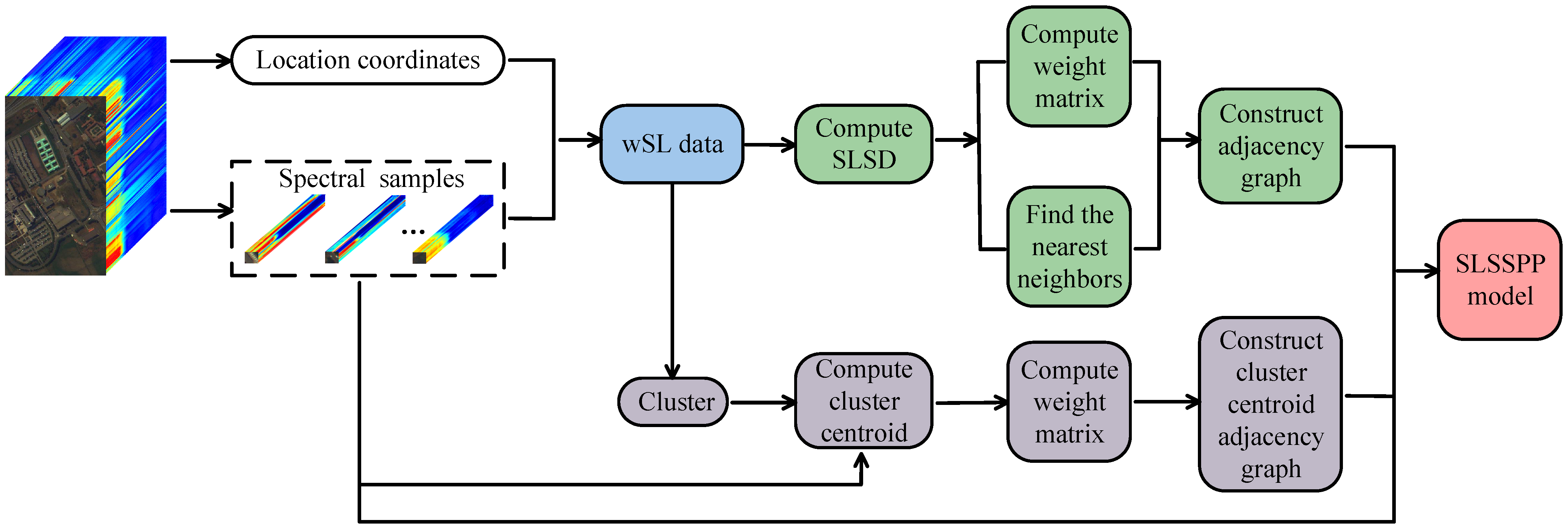
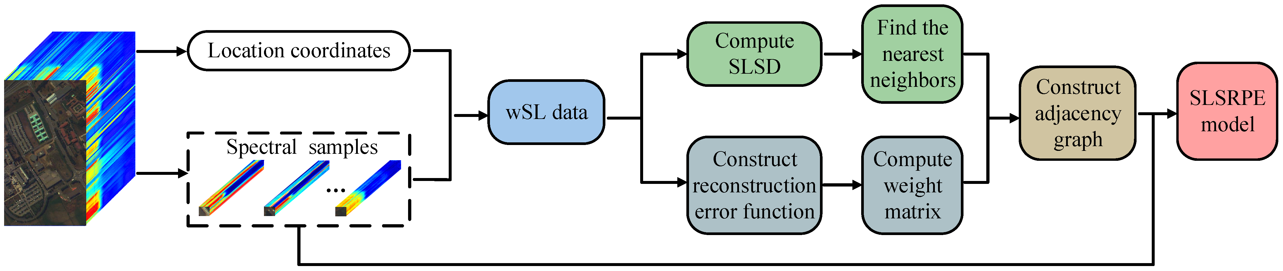
In this section, we introduce the proposed SLSD and two uSLSML methods, SLSSPP and SLSRPE, in detail. Their flowcharts are shown in Figure 1 and Figure 2. Figure 1 shows the calculation process of SLSSPP, where the first step is to generate wSL data with the location coordinates and spectral band of each pixels, which is the key to break the locality of spatial information extraction. Then, SLSD is computed based on wSL data which are also clustered to generate a clustering index. Then, based on the SLSD, SLSSPP finds k nearest neighbors and computes the weight matrix to construct the SLS adjacency graph. Meanwhile, according to the clustering index, the cluster centroid is computed based on the raw spectral data. On the basis of the cluster centroid, the weight matrix is calculated to construct the cluster centroid adjacency graph. Eventually, on account of the SLS adjacency graph and the cluster centroid adjacency graph, the SLSSPP model was built to obtain an optimal projection matrix based on the raw spectral data.

Figure 2 also shows the calculation process of SLSRPE, whose first step is also to generate wSL data with the location coordinates and spectral band of each pixel. Based on the wSL data, the second step of SLSRPE is constructing the redefined reconstruction error function to compute the redefined reconstruction weight matrix while computing SLSD to find k nearest neighbors. Then, according to the redefined reconstruction weight matrix and k nearest neighbors, the adjacency graph is constructed. Finally, the SLSRPE model is built to obtain an optimal projection matrix which is harvested to transform the original high-dimensional data into low-dimensional space. In the end, the low-dimensional features are classified by classifiers.

3.1. Spectral-Locational-Spatial Distance

In fact, SLSSPP and SLSRPE are two graph embedding methods. For an HSI dataset $\mathbf{X}=[{\mathbf{x}}_1,\dots ,{\mathbf{x}}_i,\dots ,{\mathbf{x}}_m]$ with m pixels, its adjacency graph $\mathbf{G}$ have m nodes. In general, we put an edge between nodes i and j in $\mathbf{G}$ if ${\mathbf{x}}_i$ and ${\mathbf{x}}_j$ are close (that is ${\mathbf{x}}_i$ is the nearest neighbor of ${\mathbf{x}}_j$, or ${\mathbf{x}}_j$ is the nearest neighbor of ${\mathbf{x}}_i$.). As a rule, we expect that the samples of the same class are connected and put edges when constructing $\mathbf{G}$ since the connected samples are usually required to gather or maintain a manifold structure. However, if there is a mass of connected samples belonging to different classes, the classification performance of low-dimensional features will inevitably be reduced. Accordingly, how to explore the relationship among samples and find the nearest neighbor of the same class is the key to unsupervised manifold learning. In this subsection, we propose a distance calculation method, SLSD, to measure the similarity among samples.

With the recognition of the importance of spatial information in HSI, many spectral-spatial DR methods design different spectral-spatial distance to replace the raw spectral distance but ignore the location information of pixels. Figure 3 shows the comparison of spectral bands of pixels with different locational relationships. A and B display the spectral curves of pixels that are in the same class and close to each other in location, while their spectral bands are quite different. At the same time, although the two pixels in C or D are of different kinds and located far away, their spectral curves are almost identical. In both cases, it is difficult to determine the correct pixel relationship between them based on spectral information alone. In fact, location information can alleviate this problem well since pixels that are closer to each other in location are more likely to belong to the same class, especially for HSIs covering land.

In this paper, we regard the location information as one of the attributes of pixels and utilize it to break the locality of spatial information extraction and capture more spatial information. For an HSI dataset $\mathbf{X}=[{\mathbf{x}}_1,\dots ,{\mathbf{x}}_i,\dots ,{\mathbf{x}}_m]\in {\Re }^{D\times m}$, the location information can be denoted as $\mathbf{C}=[{\mathbf{c}}_1,\dots ,{\mathbf{c}}_i,\dots ,{\mathbf{c}}_m]\in {\Re }^{2\times m}$ where ${\mathbf{c}}_i={[p_i,q_i]}^T$ is the coordinate of the pixel ${\mathbf{x}}_i$. To fuse the spectral and locational information of pixels in HSIs, a spectral-locational dataset is constructed as follows:

$${\mathbf{X}}^{\mathrm{C}}=\left[\begin{array}{c}\mathbf{C}\hfill \\ \mathbf{X}\hfill \end{array}\right]=\left[\begin{array}{c}{\mathbf{c}}_1,\dots ,{\mathbf{c}}_i,\dots ,{\mathbf{c}}_m\\ {\mathbf{x}}_1,\dots ,{\mathbf{x}}_i,\dots ,{\mathbf{x}}_m\end{array}\right]\in {\Re }^{(D+2)\times m}.$$

(7)

However, due to the difference of image size and the complexity of homogeneous domain distribution in HSIs, this simple combination of spectrum and location is not reasonable. In order to balance the effect of location and spectrum on the relationships among samples, the weighted spectral-locational (wSL) data ${\mathbf{X}}^{\mathrm{C}}=[{{\mathbf{x}}^{\mathrm{C}}}_1,\dots ,{{\mathbf{x}}^{\mathrm{C}}}_i,\dots ,{{\mathbf{x}}^{\mathrm{C}}}_m]$ are redefined as

$${\mathbf{X}}^{\mathrm{C}}=\left[\begin{array}{c}\beta \mathbf{C}\hfill \\ \left(1-\beta \right)\mathbf{X}\hfill \end{array}\right]=\left[\begin{array}{c}\beta {\mathbf{c}}_1,\dots ,\beta {\mathbf{c}}_m\\ \left(1-\beta \right){\mathbf{x}}_1,\dots ,\left(1-\beta \right){\mathbf{x}}_m\end{array}\right]$$

(8)

and ${{\mathbf{x}}^{\mathrm{C}}}_i=\left[\begin{array}{c}\beta {\mathbf{c}}_i\\ \left(1-\beta \right){\mathbf{x}}_i\end{array}\right]$. $\beta$ is a spectral-locational trade-off parameter. It needs to be emphasized that ${\mathbf{X}}^{\mathrm{C}}$ is only used to calculate the relationship among pixels, not the DR data. There is therefore no need to discuss the rationality of the physical meaning of ${\mathbf{X}}^{\mathrm{C}}$. In addition, ${\mathbf{X}}^{\mathrm{C}}$ with location also breaks the locality of spatial information extraction.

We assume the local neighborhood space of ${{\mathbf{x}}^{\mathrm{C}}}_i$ is $\mathsf{\Omega }\left({{\mathbf{x}}^{\mathrm{C}}}_i\right)$ with $s^2=1,\dots ,r$ in a $s\times s$ spatial window, which is formulated as

$$\begin{array}{c}\hfill \mathsf{\Omega }\left({{\mathbf{x}}^{\mathrm{C}}}_i\right)=\left\{{{\mathbf{x}}^{\mathrm{C}}}_i(p,q)|\begin{array}{c}p\in [p_i-\frac{s-1}{2},p_i+\frac{s-1}{2}]\\ q\in [q_i-\frac{s-1}{2},q_i+\frac{s-1}{2}]\end{array}\right\}.\end{array}$$

(9)

Actually, the primary responsibility of SLSD is to find the effective nearest neighbors. To search for highly credible neighbors, SLSD uses a local neighborhood space instead of a central sample. Accordingly, the SLSD of the sample ${\mathbf{x}}_i$ and ${\mathbf{x}}_j$ is defined as

$$\begin{array}{c}\hfill d_{\mathrm{SLSD}}\left({\mathbf{x}}_i,{\mathbf{x}}_j\right)=d\left(\mathsf{\Omega }\left({{\mathbf{x}}^{\mathrm{C}}}_i\right),{{\mathbf{x}}^{\mathrm{C}}}_j\right),\end{array}$$

(10)

where ${\mathbf{x}}_i$ is one of the neighbors of the target sample ${\mathbf{x}}_j$. $d\left(\mathsf{\Omega }\left({{\mathbf{x}}^{\mathrm{C}}}_i\right),{{\mathbf{x}}^{\mathrm{C}}}_j\right)$ is the distance between $\mathsf{\Omega }\left({{\mathbf{x}}^{\mathrm{C}}}_i\right)$ and ${{\mathbf{x}}^{\mathrm{C}}}_j$ and defined as follows:

$$\begin{array}{c}\hfill d\left(\mathsf{\Omega }\left({{\mathbf{x}}^{\mathrm{C}}}_i\right),{{\mathbf{x}}^{\mathrm{C}}}_j\right)=\frac{{\displaystyle \sum _{r=1}^{s^2}}{t}_{ir}∥{{\mathbf{x}}^{\mathrm{C}}}_j-{{\mathbf{x}}^{\mathrm{C}}}_{ir}∥}{{\displaystyle \sum _{r=1}^{s^2}}{t}_{ir}},{{\mathbf{x}}^{\mathrm{C}}}_{ir}\in \mathsf{\Omega }\left({{\mathbf{x}}^{\mathrm{C}}}_i\right),\end{array}$$

(11)

in which $t_{ir}$ is calculated by

$$\begin{array}{c}\hfill t_{ir}=exp\left(-\gamma ∥{x^C}_i-{x^C}_{ir}∥\right),{x^C}_{ir}\in \mathsf{\Omega }\left({x^C}_i\right).\end{array}$$

(12)

$\gamma$ is a constant which is empirically set to 0.2 in the experiments. The window parameter s is the size of the local spatial neighborhood $\mathsf{\Omega }\left({{\mathbf{x}}^{\mathrm{C}}}_i\right)$. ${x^C}_{ir}$ is a pixel in $\mathsf{\Omega }\left({{\mathbf{x}}^{\mathrm{C}}}_i\right)$ surrounding ${x^C}_i$. $tgir$ is the weight of ${{\mathbf{x}}^{\mathrm{C}}}_{ir}$. The more similar ${x^C}_{ir}$ is to ${x^C}_i$, the larger the value of $t_{ir}$, and the more important the distance between ${x^C}_{ir}$ and ${x^C}_j$ is. The spectral-locational trade-off parameter $\beta$ can adjust the influence of location information on distance. When $\beta =0$, SLSD is the spectral-spatial distance only based on spectral domain. When $\beta =1$, SLSD is the locational-spatial distance only based on coordinate. By choosing the appropriate $\beta$ value, we can excavate the more realistic relationships among the samples as much as possible. Furthermore, this allows the neighbor samples to be more likely to fall into the same class as the target sample. To sum up, SLSD not only extracts local spatial neighborhood information, but also explores global spatial relations in HSIs based on location information.

To illustrate the effectiveness of SLSD, we compared it with the SD and SSCD proposed in [24]. SD is the simple spectral distance and SSCD is a spectral-spatial distance without location information.

Table 1. The number of samples with different classes in the top 10 nearest neighbors of all class samples in the three datasets.

	Indian Pines			Pavia University			Salinas
Class	SD	SSCD	SLSD	SD	SSCD	SLSD	SD	SSCD	SLSD
C1	10	10	0	1120	390	0	0	0	0
C2	310	170	10	210	20	0	0	10	0
C3	220	130	0	1160	270	0	0	0	0
C4	140	100	0	720	2260	0	120	130	0
C5	20	20	0	0	180	10	90	90	40
C6	0	20	0	810	220	0	0	150	250
C7	0	0	0	620	100	0	30	40	0
C8	0	0	0	1520	410	0	2400	740	0
C9	0	0	0	0	70	0	0	0	10
C10	50	260	0				80	150	0
C11	310	160	20				10	90	80
C12	250	110	0				0	10	10
C13	10	10	0				40	20	0
C14	70	10	0				30	330	130
C15	40	0	0				2220	830	80
C16	0	60	0				0	0	20
total	1430	1060	30	6160	3920	10	5020	2590	620

shows the number of samples with different classes in the top 10 nearest neighbors of samples, which includes all samples in the three datasets. For a fair comparison, SSCD and SLSD has the same spatial window parameters for the three datasets. From Table 1, the number of samples are presented as: SLSD < SSCD < SD. This means that not only the local spatial neighborhood but also the location information are both quite valuable for the exploration of the relationship among the samples. In addition, Table 1 also shows that SLSD rarely has different classes of samples in the top 10 nearest neighbors. This means that the neighbors obtained by SLSD mostly belong to the same class as the target sample, which indicates that SLSD is excellent for correctly determining the pixel relationship in HSIs.

3.2. Spectral-Locational-Spatial Structure Preserving Projection

The core of many supervised DR algorithms to obtain discriminant projections is to shorten the intraclass distance and expand the interclass distance in low-dimensional space [14,27]. In the case of sufficient class labels, this way can indeed achieve excellent DR for classification. However, it is quite difficult to obtain class labels for HSIs covering land. In this paper, SLSSPP was proposed to approach this concept without any class labels. On account of SLSD, SLSSPP can achieve the goal of shortening the intra-class distance in an unsupervised manner, since most of the nearest neighbors belong to the same class as the target sample. Meanwhile, in SLSSPP, expanding the interclass distance is simulated by maximizing the distance among the cluster centroids based on wSL data.

With SLSD, the SLS adjacency graph ${\mathbf{G}}^{\mathrm{SLS}}=\left\{\mathbf{X},{\mathbf{W}}^{\mathrm{SLS}}\right\}$ can be constructed, where $\mathbf{X}$ is the vertex of the graph and ${\mathbf{W}}^{\mathrm{SLS}}$ is the weight matrix. In graph ${\mathbf{G}}^{\mathrm{SLS}}$, if ${\mathbf{x}}_j$ belongs to the k nearest neighbors $N_k^{\mathrm{SLS}}\left({\mathbf{x}}_i\right)$ of ${\mathbf{x}}_i$ based on SLSD, an edge should be connected between them. In this paper, if ${\mathbf{x}}_i\in N_k^{\mathrm{SLS}}\left({\mathbf{x}}_j\right)$ or ${\mathbf{x}}_j\in N_k^{\mathrm{SLS}}\left({\mathbf{x}}_i\right)$, the weight of each edge is defined as

$$\begin{array}{c}\hfill w_{ij}^{\mathrm{SLS}}=exp(-\frac{d_{\mathrm{SLSD}}{\left({\mathbf{x}}_i,{\mathbf{x}}_j\right)}^2}{2{t_i}^2}),\end{array}$$

(13)

where:

$$\begin{array}{c}\hfill t_i=\frac{1}{k}\sum _{{\mathbf{x}}_j\in N_k^{\mathrm{SLS}}\left({\mathbf{x}}_i\right)}{d}_{\mathrm{SLSD}}\left({\mathbf{x}}_i,{\mathbf{x}}_j\right).\end{array}$$

(14)

Otherwise, $w_{ij}^{\mathrm{SLS}}=0$. $d_{\mathrm{SLSD}}({\mathbf{x}}_i,{\mathbf{x}}_j)$ is the SLSD between ${\mathbf{x}}_i$ and ${\mathbf{x}}_j$. Due to the superior performance of SLSD in representing the relationship among samples in HSIs, ${\mathbf{W}}^{\mathrm{SLS}}$ based on SLSD can make the low-dimensional space keep the more real structure of the raw space. Actually, $k<<m$, therefore ${\mathbf{W}}^{\mathrm{SLS}}$ is a sparse matrix.

In order to shorten the distance among each sample and its k nearest neighbors in embedding space, the optimization problem is defined as

$$\begin{array}{c}\hfill \begin{array}{c}\underset{\mathbf{V}}{min}{\displaystyle \sum _{i,j}^m}\parallel {\displaystyle \frac{1}{2}}\left({\mathbf{V}}^T{\mathbf{x}}_i-{\mathbf{V}}^T{\mathbf{x}}_j\right){\parallel }^2{w}_{ij}^{\mathrm{SLS}}={\displaystyle \sum _i^m}{\mathbf{V}}^T{\mathbf{x}}_i{D}_{ii}^{\mathrm{SLS}}{\mathbf{x}}_i^T\mathbf{V}-{\displaystyle \sum _{i,j}^m}{\mathbf{V}}^T{\mathbf{x}}_i{w}_{ij}^{\mathrm{SLS}}{\mathbf{x}}_j^T\mathbf{V}\hfill \\ =\mathrm{t}r\left({\mathbf{V}}^T\mathbf{X}\left({\mathbf{D}}^{\mathrm{SLS}}-{\mathbf{W}}^{\mathrm{SLS}}\right){\mathbf{X}}^T\mathbf{V}\right)\hfill \\ =\mathrm{t}r\left({\mathbf{V}}^T\mathbf{X}{\mathbf{L}}^{SLS}{\mathbf{X}}^T\mathbf{V}\right)\hfill \end{array},\end{array}$$

(15)

in which ${\mathbf{W}}^{\mathrm{SLS}}$ is a symmetric matrix and ${\mathbf{D}}^{\mathrm{SLS}}$ is a diagonal matrix whose entries are column or row sums of ${\mathbf{W}}^{\mathrm{SLS}}$, $D_{ii}^{\mathrm{SLS}}={\sum }_j{w}_{ij}^{\mathrm{SLS}}$. ${\mathbf{L}}^{\mathrm{SLS}}={\mathbf{D}}^{\mathrm{SLS}}-{\mathbf{W}}^{\mathrm{SLS}}$ is the Laplacian matrix. In addition, it can be further evolved to:

$$\begin{array}{c}\hfill \underset{\mathbf{V}}{min}{\mathbf{V}}^T\mathbf{X}{\mathbf{L}}^{\mathrm{SLS}}{\mathbf{X}}^T\mathbf{V}.\end{array}$$

(16)

To indirectly expand the interclass distance, we maximize the distance among cluster centroids.

Table 2. The number of heterogeneous samples in the same cluster when three datasets are divided into 35 clusters.

	Indian Pines	Pavia University	Salinas
Spectral-locational data	2063	4055	3333
Raw spectral data	4054	9936	8164

shows the number of heterogeneous samples in the same cluster when three datasets are divided into 35 clusters. Compared with the raw spectral datum $\mathbf{X}$, the wSL datum ${\mathbf{X}}^{\mathrm{C}}$ has better clustering performance. This means that ${\mathbf{X}}^{\mathrm{C}}$ should be used to compute the cluster index that guide the low-dimensional features. To facilitate the implementation and calculation, we adopt K-means algorithm to cluster ${\mathbf{X}}^{\mathrm{C}}$. Assuming ${\mathbf{X}}^{\mathrm{C}}$ is divided into $km$ clusters, the index $F=[f_1,\dots ,f_i,\dots ,f_{km}]$ of $km$ clusters can be obtained as follows:

$$\begin{array}{c}\hfill F=\mathrm{Kmeans}({\mathbf{X}}^C,km),\end{array}$$

(17)

where $\mathrm{Kmeans}\left(\right)$ is the K-means algorithm and $f_i$ is the sample index belonging to the i-th cluster. According to the index F, the cluster centroid $\mathbf{U}=[{\mathbf{u}}_1,\dots ,{\mathbf{u}}_i,\dots ,{\mathbf{u}}_{km}]$ of $\mathbf{X}$ is calculated as

$$\begin{array}{c}\hfill {\mathbf{u}}_i=\sum _{j\in f_i}{\mathbf{x}}_j.\end{array}$$

(18)

The optimization problem of cluster centroid distance maximization is defined as

$$\begin{array}{c}\hfill \begin{array}{c}\underset{\mathbf{V}}{max}{\displaystyle \sum _{i,j}^{km}}{\parallel {\displaystyle \frac{1}{2}}\left({\mathbf{V}}^T{\mathbf{u}}_i-{\mathbf{V}}^T{\mathbf{u}}_j\right)\parallel }^2{w}_{ij}^{\mathrm{C}}={\displaystyle \sum _{i,j}^{km}}{\mathbf{V}}^T{\mathbf{u}}_i{D}_{ii}^{\mathrm{C}}{\mathbf{u}}_j^T\mathbf{V}-{\displaystyle \sum _{i,j}^{km}}{\mathbf{V}}^T{\mathbf{u}}_i{w}_{ij}^{\mathrm{c}}{\mathbf{u}}_j^T\mathbf{V}\hfill \\ =tr\left({\mathbf{V}}^T\mathbf{U}\left({\mathbf{D}}^{\mathrm{C}}-{\mathbf{W}}^{\mathrm{C}}\right){\mathbf{U}}^T\mathbf{V}\right)\hfill \\ =tr\left({\mathbf{V}}^T\mathbf{U}{\mathbf{L}}^{\mathrm{C}}{\mathbf{U}}^T\mathbf{V}\right)\hfill \end{array}\end{array}$$

(19)

Here, ${\mathbf{W}}^{\mathrm{C}}$ is the weight matrix of the cluster centroid, which is defined as

$$\begin{array}{c}\hfill w_{ij}^{\mathrm{c}}={(1+exp(-\frac{d_{\mathrm{E}}{\left({\mathbf{u}}_i,{\mathbf{u}}_i\right)}^2}{2{t_i}^2}))}^{-1},t_i=\frac{1}{km}\sum _j^{km}{d}_{\mathrm{E}}\left({\mathbf{u}}_i,{\mathbf{u}}_j\right),{\mathbf{u}}_i=\sum _{j\in f_i}{\mathbf{x}}_j.\end{array}$$

(20)

$d_{\mathrm{E}}\left(\right)$ is the Euclidean distance function. The definition of ${\mathbf{W}}^{\mathrm{C}}$ means that the greater the distance between cluster centroid ${\mathbf{u}}_i^r$ and ${\mathbf{u}}_j^r$, the greater the weight $w_{ij}^{\mathrm{c}}$, and thus the greater the degree of separation between cluster i and j in low-dimensional space, and vice versa. ${\mathbf{W}}^{\mathrm{C}}$ is a symmetric matrix and $D_{ii}^{\mathrm{C}}={\sum }_j{w}_{ij}^{\mathrm{c}}$. This optimization problem can be further evolved to:

$$\begin{array}{c}\hfill \underset{\mathbf{V}}{max}{\mathbf{V}}^T\mathbf{U}{\mathbf{L}}^{\mathrm{C}}{\mathbf{U}}^T\mathbf{V}\end{array}$$

(21)

Aiming to simultaneously minimize the distance among each sample and its k nearest neighbors and maximize the distance among cluster centroids to obtain the discriminant low-dimensional representations, the DR model of SLSSPP is defined as

$$\begin{array}{c}\hfill J\left(\mathbf{V}\right)=max\frac{{\mathbf{V}}^T\mathbf{U}{\mathbf{L}}^{\mathrm{C}}{\mathbf{U}}^T\mathbf{V}}{{\mathbf{V}}^T\mathbf{X}{\mathbf{L}}^{\mathrm{SLS}}{\mathbf{X}}^T\mathbf{V}}.\end{array}$$

(22)

As a general rule, this equals to the following optimization program:

$$\begin{array}{c}\hfill \left\{\begin{array}{c}\underset{\mathbf{V}}{max}{\mathbf{V}}^T\mathbf{U}{\mathbf{L}}^{\mathrm{C}}{\mathbf{U}}^T\mathbf{V}\hfill \\ s.t.{\mathbf{V}}^T\mathbf{X}{\mathbf{L}}^{\mathrm{SLS}}{\mathbf{X}}^T\mathbf{V}=\mathbf{Z}\hfill \end{array}\right.\end{array}$$

(23)

where $\mathbf{Z}$ is a non-zero constant matrix. Based on the Lagrangian multipliers, the optimization solution can be obtained through the following generalized eigenvalue problem:

$$\begin{array}{c}\hfill \mathbf{U}{\mathbf{L}}^{\mathrm{C}}{\mathbf{U}}^T\mathbf{V}=\lambda \mathbf{X}{\mathbf{L}}^{\mathrm{SLS}}{\mathbf{X}}^T\mathbf{V}\Rightarrow {\left(\mathbf{X}{\mathbf{L}}^{\mathrm{SLS}}{\mathbf{X}}^T\right)}^{-1}\mathbf{U}{\mathbf{L}}^{\mathrm{C}}{\mathbf{U}}^T\mathbf{V}=\lambda \mathbf{V}\end{array}$$

(24)

where $\lambda$ is the eigenvalue of Equation (24). With the eigenvectors ${\mathbf{v}}_1,{\mathbf{v}}_2,\dots ,{\mathbf{v}}_d$ corresponding to the d largest eigenvalues, the optimal projection matrix can be represented as

$$\begin{array}{c}\hfill \mathbf{V}=[{\mathbf{v}}_1,{\mathbf{v}}_2,\dots ,{\mathbf{v}}_d]\in {\Re }^{D\times d}\end{array}$$

(25)

Finally, the low-dimensional embedding dataset can be given by $\mathbf{Y}={\mathbf{V}}^T\mathbf{X}\in {\Re }^{d\times m}$.

The detailed procedure of SLSSPP is given in Algorithm 1. In general, SLSSPP has two contributions: (1) it takes advantage of SLSD to search the nearest neighbor and construct an adjacency graph; and (2) a cluster centroid adjacency graph based on wSL data is constructed. In order to demonstrate their superiority in dimensionality reduction, the comparative experiments based on three datasets are carried out and the classification overall accuracies (OAs) are shown in

Table 3. Classification OAs of the embedding features (dim = 30) of different algorithms under different training conditions of the two classifiers.

Dataset	${\mathit{n}}_{\mathit{i}}$	5		10		20		30		40		60
	Classifiers	KNN	SVM	KNN	SVM	KNN	SVM	KNN	SVM	KNN	SVM	KNN	SVM
Indian	LPP	69.4	72.2	76.8	80.0	85.3	86.7	88.2	90.3	90.2	92.3	92.9	93.7
	LPP_Cluster	73.6	76.4	83.1	84.2	89.4	91.5	91.3	92.8	93.2	94.1	95.0	95.5
	LPP_SLSD	82.1	82.9	89.9	89.6	94.4	94.5	96.3	96.4	97.8	96.8	98.3	97.9
	SLSSPP	84.1	82.7	93.1	92.0	96.0	95.2	96.7	96.1	98.0	96.5	98.3	97.8
Pavia U	LPP	67.2	68.6	74.3	81.0	83.6	88.6	86.9	91.5	88.8	93.7	90.9	94.3
	LPP_Cluster	68.6	79.5	77.7	88.8	83.6	92.6	85.6	93.7	87.7	95.4	89.5	96.0
	LPP_SLSD	82.6	72.9	91.1	82.8	93.5	91.3	95.4	94.0	96.6	94.7	97.0	96.2
	SLSSPP	82.6	86.7	90.6	89.6	93.9	93.4	95.8	95.3	96.3	95.3	97.5	96.5
Salinas	LPP	89.2	88.3	91.1	90.8	92.8	93.1	94.0	94.1	94.8	94.7	95.2	95.6
	LPP_Cluster	91.7	92.6	93.2	93.5	95.2	95.1	95.7	96.1	95.8	95.5	96.7	97.3
	LPP_SLSD	93.6	92.8	94.7	93.9	96.6	95.8	97.3	96.1	97.8	96.3	98.3	97.6
	SLSSPP	93.5	94.6	94.7	94.4	96.7	95.7	97.1	96.1	97.7	97.0	98.3	97.1

where $n_i$ is the number of training samples per class used for the classifiers. The LPP_Cluster represents the combination of LPP and the cluster centroid adjacency graph, while LPP_SLSD represents that traditional LPP uses SLSD to explore the nearest neighbor and construct adjacency graph. From Table 3, both LPP_Cluster and LPP_SLSD outperform traditional LPP under different training conditions of the two classifiers, which means that both designs in SLSSPP are valid. In fact, based on these two designs, the SLSSPP model in Equation (22) can indirectly reduce the intraclass distance and increase the interclass distance in an unsupervised manner, which not only preserves the neighborhood structure of HSIs, but also effectively enhances the separability of low-dimensional embeddings. Table 3 also shows that SLSSPP has better classification performance than LPP_Cluster and LPP_SLSD, which indicates that the proposed SLSSPP is quite meaningful.

Algorithm 1 SLSSPP

Input: A D-dimensional HSI dataset $\mathbf{X}=[{\mathbf{x}}_1,\dots ,{\mathbf{x}}_i,\dots ,{\mathbf{x}}_m]\in {\Re }^{D\times \mathrm{m}}$, nearest neighbors number $k>0$, spatial window size $s>0$, embedding dimension d$(d<D)$ and trade-off parameter $0\le \beta \le 1$. 1: Obtain location information $\mathbf{C}$ and generate wSL data ${\mathbf{X}}^{\mathrm{C}}$ as Equation (8). 2: Compute the SLSD $d_{\mathrm{SLSD}}({\mathbf{x}}_i,{\mathbf{x}}_j)$ among samples by Equations (10)–(12). 3: Find the k nearest neighbors $N_k^{\mathrm{SLS}}\left({\mathbf{x}}_i\right)$ of each samples ${\mathbf{x}}_i$ based on SLSD. 4: Compute the weight matrix ${\mathbf{W}}^{\mathrm{SLS}}$ in adjacency graph by Equations (13) and (14). 5: Compute the cluster centroid index F by Equation (17) and the cluster centroid $\mathbf{U}$ by Equation (18). 6: Compute the weight matrix of the cluster centroid ${\mathbf{W}}^{\mathrm{C}}$ by Equation (20). 7: Construct the DR model $J\left(\mathbf{V}\right)$ as Equation (22) and solve the generalized eigenvalue problem as Equation (24). 8: Obtain the projection matrix with the d largest eigenvalues corresponding eigenvectors: $\mathbf{V}=[{\mathbf{v}}_1,\dots ,{\mathbf{v}}_d]\in {\Re }^{D\times d}$. Output:$\mathbf{Y}={\mathbf{V}}^T\mathbf{X}\in {\Re }^{d\times m}$

3.3. Spectral-Locational-Spatial Reconstruction Preserving Embedding

From Section 2.2, NPE constructs the reconstruction error function simply based on the spectral information, which is unreliable not only due to the spectral redundancy and noise in HSIs, but also because different objects may share the same spectral properties. To address this problem, SLSRPE redefines an SLS reconstruction error function to compute the SLS reconstruction weights, which is based on the wSL data instead of the raw spectral data. In addition, the SLS reconstruction weights also consider the contribution of local spatial neighborhood.

Based on SLSD, the adjacency graph ${\mathbf{G}}^{\mathrm{RPE}}=\left\{\mathbf{X},{\mathbf{W}}^{\mathrm{RPE}}\right\}$ is constructed. ${\mathbf{W}}^{\mathrm{RPE}}$ is the reconstruction weight matrix. The superiority of SLSD in finding the nearest neighbor proves that SLS information is quite beneficial to characterize the relationship among samples. As a result, SLS information should be used to construct the reconstruction error function and calculate the reconstruction weight. In fact, the closer the SLS relationship is, the more probable it is that the selected neighbor has the same class as the target sample, and the greater its reconstruction weight will be. In this way, the reconstruction error function for the optimal weights is redefined as follows:

$$\begin{array}{c}\hfill \left\{\begin{array}{c}\underset{w_{ij}^{\mathrm{RPE}}}{min}{\displaystyle \sum _{i=1}^m}\parallel {\displaystyle \sum _{j=1}^k}{w}_{ij}^{\mathrm{RPE}}\frac{{\displaystyle \sum _{r=1}^{s^2}}{t}_{jr}\left({{\mathbf{x}}^{\mathrm{C}}}_i-{{\mathbf{x}}^{\mathrm{C}}}_{jr}\right)}{{\displaystyle \sum _{r=1}^{s^2}}{t}_{jr}}{\parallel }^2\hfill \\ s.t.{\displaystyle \sum _{j=1}^m}{w}_{ij}^{\mathrm{RPE}}=1\hfill \\ s.t.w_{ij}^{RPE}=0,\forall {\mathbf{x}}_j\notin N_k^{\mathrm{SLS}}\left({\mathbf{x}}_i\right)\hfill \end{array}\right.,\end{array}$$

(26)

in which ${{\mathbf{x}}^{\mathrm{C}}}_{jr}\in \mathsf{\Omega }\left({{\mathbf{x}}^{\mathrm{C}}}_j\right)$ is the local spatial neighbor of ${{\mathbf{x}}^C}_j$ and $t_{jr}=exp(-2d_{\mathrm{SLSD}}{\left({\mathbf{x}}_j,{\mathbf{x}}_{jr}\right)}^2)$. $d_{\mathrm{SLSD}}\left({\mathbf{x}}_j,{\mathbf{x}}_{jr}\right)$ is the SLSD between ${\mathbf{x}}_j$ and ${\mathbf{x}}_{jr}$. The more similar ${\mathbf{x}}_{jr}$ is to ${\mathbf{x}}_j$, the greater the contribution ${\mathbf{x}}_{jr}$ makes to the relationship between ${\mathbf{x}}_j$ and ${\mathbf{x}}_i$, which improves the robustness of reconstructed weights to noisy samples. By solving the reconstruction error function, we obtain the reconstructed weight matrix ${\mathbf{W}}^{\mathrm{RPE}}$.

Supposing that ${\mathbf{x}}_{ij}$ is the jth nearest neighbor of ${\mathbf{x}}_i$ based on SLSD, k is the number of the selected nearest neighbors, ${{\mathbf{x}}^{\mathrm{C}}}_{ijr}$ is the rth local spatial neighbor of ${{\mathbf{x}}^{\mathrm{C}}}_{ij}$. For the sake of explanation:

$$\begin{array}{c}\hfill h_{ij}=\frac{{\displaystyle \sum _{r=1}^{s^2}}{t}_{ijr}\left({{\mathbf{x}}^{\mathrm{C}}}_i-{{\mathbf{x}}^{\mathrm{C}}}_{ijr}\right)}{{\displaystyle \sum _{r=1}^{s^2}}{t}_{ijr}}\end{array}$$

(27)

indicates the SLS combined measure between ${\mathbf{x}}_i$ and ${\mathbf{x}}_{ij}$. The reconstruction error function can be simplified to:

$$\begin{array}{c}\hfill min\sum _{i=1}^m\parallel \sum _{j=1}^k{w}_{ij}^{\mathrm{RPE}}{h}_{ij}{\parallel }^2=min\sum _{i=1}^m{\left({\mathbf{w}}_i^{\mathrm{RPE}}\right)}^T{\mathbf{z}}_i{\mathbf{w}}_i^{\mathrm{RPE}}\end{array}$$

(28)

where ${\mathbf{z}}_i={[h_{i1},\dots ,h_{ij},\dots ,h_{ik}]}^T[h_{i1},\dots ,h_{ij},\dots ,h_{ik}]$ and ${\mathbf{w}}_i^{\mathrm{RPE}}=[w_{i1}^{\mathrm{RPE}},\dots ,w_{ij}^{\mathrm{RPE}},\dots ,w_{ik}^{\mathrm{RPE}}]$. Then, the reconstruction error function can be expressed as the following optimization problem:

$$\begin{array}{c}\hfill \left\{\begin{array}{c}\underset{w_{ij}^{\mathrm{RPE}}}{min}{\displaystyle \sum _{i=1}^m}{\left({\mathbf{w}}_i^{\mathrm{RPE}}\right)}^T{\mathbf{z}}_i{\mathbf{w}}_i^{\mathrm{RPE}}\hfill \\ s.t.{\displaystyle \sum _{j=1}^k}{w}_{ij}^{\mathrm{RPE}}=1\hfill \end{array}\right.\end{array}$$

(29)

with the Lagrange multiplier method, $w_{ij}^{\mathrm{RPE}}$ is given as follows:

$$\begin{array}{c}\hfill w_{ij}^{\mathrm{RPE}}=\frac{{\displaystyle \sum _{l=1}^k}{\left({\mathbf{z}}_i^{jl}\right)}^{-1}}{{\displaystyle \sum _{p,q=1}^k}{\left({\mathbf{z}}_i^{pq}\right)}^{-1}}\end{array}$$

(30)

where ${\mathbf{z}}_i^{jl}={\left({\mathbf{h}}_{ij}\right)}^T{\mathbf{h}}_{il}$ and ${\mathbf{z}}_i^{pq}={\left({\mathbf{h}}_{ip}\right)}^T{\mathbf{h}}_{iq}$. $w_{ij}^{\mathrm{RPE}}$ is the reconstruction coefficient of ${\mathbf{x}}_j$ to ${\mathbf{x}}_i$. In fact, $k<<m$, so the reconstruction matrix ${\mathbf{W}}^{\mathrm{RPE}}$ is a sparse matrix. According to ${\mathbf{W}}^{\mathrm{RPE}}$, SLSRPE maintains the reconstructed relationship between the target sample and the nearest neighbors in a low-dimensional space. The DR model of SLSRPE is defined as

$$\begin{array}{c}\hfill \left\{\begin{array}{c}\underset{\mathbf{V}}{min}{\displaystyle \sum _i^m}|{\mathbf{V}}^T{\mathbf{x}}_i-{\displaystyle \sum _j^m}{w}_{ij}^{\mathrm{RPE}}{\mathbf{V}}^T{\mathbf{x}}_j{\parallel }^2\hfill \\ s.t.{\displaystyle \sum _i^m}{\mathbf{V}}^T{\mathbf{x}}_i=0,{\displaystyle \frac{1}{m}}\mathbf{V}{\mathbf{V}}^T=\mathbf{I}\hfill \end{array}\right.,\end{array}$$

(31)

which can be reduced as

$$\begin{array}{c}\hfill \begin{array}{c}\underset{\mathbf{V}}{min}{\displaystyle \sum _i^m}\parallel {\mathbf{V}}^T{\mathbf{x}}_i-{\displaystyle \sum _j^m}{w}_{ij}^{\mathrm{RPE}}{\mathbf{V}}^T{\mathbf{x}}_j{\parallel }^2=\underset{\mathbf{V}}{min}{\displaystyle \sum _i^m}{\parallel {\displaystyle \sum _j^m}{w}_{ij}^{\mathrm{RPE}}({\mathbf{V}}^T{\mathbf{x}}_i-{\mathbf{V}}^T{\mathbf{x}}_j)\parallel }^2\hfill \\ =\underset{\mathbf{V}}{min}\mathrm{t}r\left({\mathbf{V}}^T\mathbf{X}(\mathbf{I}-{\mathbf{W}}^{\mathrm{RPE}}){(\mathbf{I}-{\mathbf{W}}^{\mathrm{RPE}})}^T{\mathbf{X}}^T\mathbf{V}\right)\hfill \\ =\underset{\mathbf{V}}{min}{\mathbf{V}}^T\mathbf{X}{\mathbf{M}}^{\mathrm{RPE}}{\mathbf{X}}^T\mathbf{V}\hfill \end{array},\end{array}$$

(32)

where ${\mathbf{M}}^{\mathrm{RPE}}=(\mathbf{I}-{\mathbf{W}}^{\mathrm{RPE}}){(\mathbf{I}-{\mathbf{W}}^{\mathrm{RPE}})}^T$ and $\mathbf{I}=\mathrm{diag}[1,\dots ,1]$. Equation (32) can be solved by the Lagrange multiplier, and it can be transformed into the following form:

$$\begin{array}{c}\hfill \mathbf{X}{\mathbf{M}}^{\mathrm{RPE}}{\mathbf{X}}^T\mathbf{V}=\lambda \mathbf{X}{\mathbf{X}}^T\mathbf{V}\Rightarrow {\left(\mathbf{X}{\mathbf{X}}^T\right)}^{-1}\mathbf{X}{\mathbf{M}}^{\mathrm{RPE}}{\mathbf{X}}^T\mathbf{V}=\lambda \mathbf{V},\end{array}$$

(33)

where $\lambda$ is the eigenvalue of Equation (33). With the eigenvectors ${\mathbf{v}}_1,{\mathbf{v}}_2,\dots ,{\mathbf{v}}_d$ corresponding to the d smallest eigenvalues, the optimal projection matrix can be represented by $\mathbf{V}=[{\mathbf{v}}_1,{\mathbf{v}}_2,\dots ,{\mathbf{v}}_d]\in {\Re }^{D\times d}$. Finally, the low-dimensional embeddings can be given by $\mathbf{Y}={\mathbf{V}}^T\mathbf{X}\in {\Re }^{d\times m}$.

The detailed procedure of the presented SLSRPE approach is given in Algorithm 2. In contrast to traditional NPE, SLSRPE also has two contributions: (1) it takes advantage of SLSD to search the nearest neighbor, (2) it redefines the reconstruction error function to calculate the reconstruction weight matrix. Both of these include an integrated exploration of spectral-locational-spatial information. To demonstrate their effectiveness separately, we conducted experiments on three datasets, and the experimental results are shown in

Table 4. Classification OAs of the embedding features (dim = 30) of different algorithms under different training conditions of the two classifiers.

Dataset	${\mathit{n}}_{\mathit{i}}$	5		10		20		30		40		60
	Classifiers	KNN	SVM	KNN	SVM	KNN	SVM	KNN	SVM	KNN	SVM	KNN	SVM
Indian	NPE	69.4	72.6	77.3	79.9	85.2	86.3	88.3	89.9	90.0	91.9	93.0	93.7
	NPE_SLS	78.9	78.9	85.7	86.6	90.5	91.8	93.1	93.2	95.0	95.1	96.2	96.3
	NPE_SLSD	77.2	78.4	83.8	87.1	89.4	91.0	91.6	92.7	93.4	94.5	95.1	95.9
	SLSRPE	88.1	86.4	92.0	91.5	97.3	94.1	97.1	95.5	98.4	96.8	98.9	97.4
Pavia U	NPE	58.2	66.5	63.7	79.6	73.4	86.8	76.7	90.2	80.8	93.3	83.8	93.9
	NPE_SLS	85.6	74.4	91.4	83.3	94.6	89.0	96.0	93.5	96.5	95.9	97.2	96.5
	NPE_SLSD	64.4	72.3	72.6	80.9	78.2	88.9	82.0	92.7	84.3	93.4	87.0	95.2
	SLSRPE	87.7	77.4	92.4	85.9	96.2	90.7	96.3	93.6	96.9	95.1	97.7	96.3
Salinas	NPE	81.6	85.5	85.2	89.9	87.3	91.3	88.0	92.9	88.5	94.4	90.1	95.0
	NPE_SLS	90.8	89.0	93.3	92.4	94.4	94.1	96.1	95.0	96.4	95.3	97.3	96.3
	NPE_SLSD	83.8	89.9	86.5	91.3	89.9	92.9	89.4	95.1	89.9	95.5	90.4	96.1
	SLSRPE	91.4	90.2	95.9	92.3	96.1	93.9	97.0	94.7	97.3	95.1	98.1	96.4

. NPE_SLS is used to test our proposed reconstruction weights that contain SLS information, while NPE_SLSD indicates that traditional NPE uses SLSD to search the nearest neighbors. From Table 4, both NPE_SLS and NPE_SLSD are superior to traditional NPE. Even more, NPE_SLS has advantages over NPE_SLSD. This means that the two points proposed in SLSRPE are meaningful, and that the reconstruction weights we redefine to include the SLS information are valuable. Accordingly, SLSRPE explores reconstruction relationships among samples not only in spectral domain, but also based on the location and local spatial neighborhood. SLSRPE makes full use of spectral-locational-spatial information of HSIs to obtain discriminating features to improve the classification performance. In fact, Table 4 also shows that SLSRPE is superior to NPE_SLS and NPE_SLSD.

Algorithm 2 SLSRPE

Input: A D-dimensional HSI dataset $\mathbf{X}=[{\mathbf{x}}_1,\dots ,{\mathbf{x}}_i,\dots ,{\mathbf{x}}_m]\in {\Re }^{D\times \mathrm{m}}$, nearest neighbors number $k>0$, spatial window size $s>0$, embedding dimension d$(d<D)$ and trade-off parameter $0\le \beta \le 1$. 1: Obtain location information $\mathbf{C}$ and generate wSL data ${\mathbf{X}}^{\mathrm{C}}$ as Equation (8). 2: Compute the SLSD $d_{\mathrm{SLSD}}({\mathbf{x}}_i,{\mathbf{x}}_j)$ by Equations (10)–(12). 3: Find the k nearest neighbors $N_k^{SLS}\left({\mathbf{x}}_i\right)$ of each samples ${\mathbf{x}}_i$ based on SLSD. 4: Construct the reconstruction error function as Equation (26). 5: Compute the reconstruction weight $w_{ij}^{\mathrm{RPE}}$ by Equation (30). 6: Solve the generalized eigenvalue problem as Equation (33). 7: Obtain the projection matrix with the d smallest eigenvalues corresponding eigenvectors: $\mathbf{V}=[{\mathbf{v}}_1,\dots ,{\mathbf{v}}_d]\in {\Re }^{D\times d}$. Output: $\mathbf{Y}={\mathbf{V}}^T\mathbf{X}\in {\Re }^{d\times m}$

4. Experiments

4.1. Description of Datasets

The first dataset covers the University of Pavia, Northern Italy, which was acquired by ROSIS sensor and called the PaviaU Dataset. Its spectral range is 0.4–0.82 $\mathsf{\mu }$m. After removing 12 noise bands from the original dataset with 115 spectral bands, 103 bands were employed in this paper. The spatial resolution is 1.3 m and each band has $610\times 340$ pixels. This dataset consists of nine ground-truth classes with 42,776 pixels and a background with 164,624 pixels. Figure 4a,b show the color image and the labeled image with nine classes.

The second dataset, Salinas Dataset, covering Salinas Vally, CA, was acquired by AVIRIS sensor in 1998, whose spatial resolution is 3.7 m. There are 224 original bands with spectral ranging from 0.4 to 2.45 $\mathsf{\mu }$m. Each band has $512\times 217$ pixels including 16 ground-truth classes with 56,975 pixels and a background with 54,129 pixels. The color image and the labeled image with 16 classes are shown in Figure 4c,d.

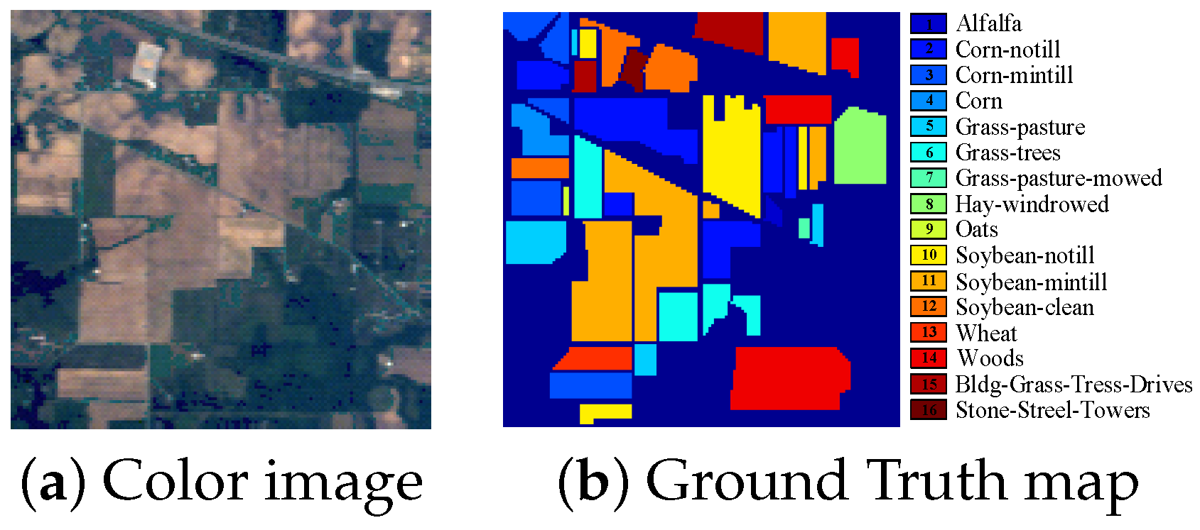
The third dataset, Indian Pines Dataset, covering the Indian Pines region, northwest Indiana, USA, was acquired by AVIRIS sensor in 1992. The spatial resolution of this image is 20 m. It has 220 original spectral bands in the 0.4–2.5 $\mathsf{\mu }$m spectral region and each band contains $145\times 145$ pixels. Owing to the noise and water absorption, 104–108, 150–163 and 220 spectral bands were abandoned and the remaining 200 bands are used in this dataset. This dataset contains background with 10,776 pixels and 16 ground-truth classes with 10,249 pixels. The number of pixels in each class ranges from 20 to 2455. The color image and the labeled image with 16 classes are shown in Figure 5.

4.2. Experimental Setup

In order to verify the superiority of two uSLSML methods, seven state-of-art DR algorithms were selected for comparison, including NPE [21], LPP [20], regularized local discriminant embedding (RLDE) [14], LPNPE [14], spatial and spectral RLDE (SSRLDE) [14], SSMRPE [24], and SSLDP [27]. The former three methods are spectral-based DR methods, while the latter four approaches make use of both spatial and spectral information for the DR of HSIs. In addition, the raw spectral feature of HSIs is also used for comparison. SSRLDE has single-scale and multi-scale versions, and we select its single-scale version because SLSSPP and SLSRPE are two single-scale models. SSMRPE [24] proposes a new SSCD to construct the spatial-spectral adjacency graph to reveal the intrinsic manifold structure of HSIs. Among them, RLDE, SSRLDE [14], and SSLDP [27] are three supervised methods and require class labels to implement DR, while others are unsupervised.

Two classifiers, support vector machines (SVMs) and k nearest neighbors (KNNs), are applied to the classification of low-dimensional features. In this paper, we utilized the one nearest neighbor and LibSVM toolbox with a radial basis function. In all experiments, we randomly divided each HSI dataset into training and test sets. It should be emphasized that the training set used for training the DR model and classifier in supervised algorithm was only used to train the classifier in unsupervised algorithm. For unsupervised methods in all experiments, all samples in an HSI dataset are utilized to train the DR model. The test set was projected into the low-dimensional space for classification. The classification overall accuracy (OA), the average accuracy (AA), and the Kappa coefficient $\kappa$ are used to evaluate classification performance.

To achieve good classification results, we optimized the parameters of various algorithms. For LPP [20] and NPE [21], the number of nearest neighbors k was set to 7 on Indian Pines dataset, 25 on PaviaU and Salinas datasets. We chose the optimal parameters of their source literature for other comparison algorithms. For RLDE, LPNPE and SSRLDE [14], the number of intraclass and interclass neighbors are both 5, the heat kernel parameter is 0.5, the parameters $\alpha$, $\beta$ and neighborhood scale are set to 0.1, 0.1, 11 on the Indian Pines and Salinas datasets, and 0.2, 0.3, 7 on the PaviaU dataset. For SSMRPE [24], the spatial window size and neighbor number are set to 7, 10 on Indian Pines dataset, 13, 20 on PaviaU dataset, 15, 15 on Salinas dataset. For SSLDP [27], the intraclass and interclass neighbor number, spatial neighborhood scale and trade-off parameter are set to 7, 63, 15, 0.6 on the Indian Pines and Salinas datasets, and 6, 66, 19, 0.4 on the PaviaU dataset. To reduce the influence of noise in HSIs, the weighted mean filtering with the $5\times 5$ window is used to preprocess the pixels. In addition, each experiment in this paper is repeated 10 times in each condition for reducing the experimental random error.

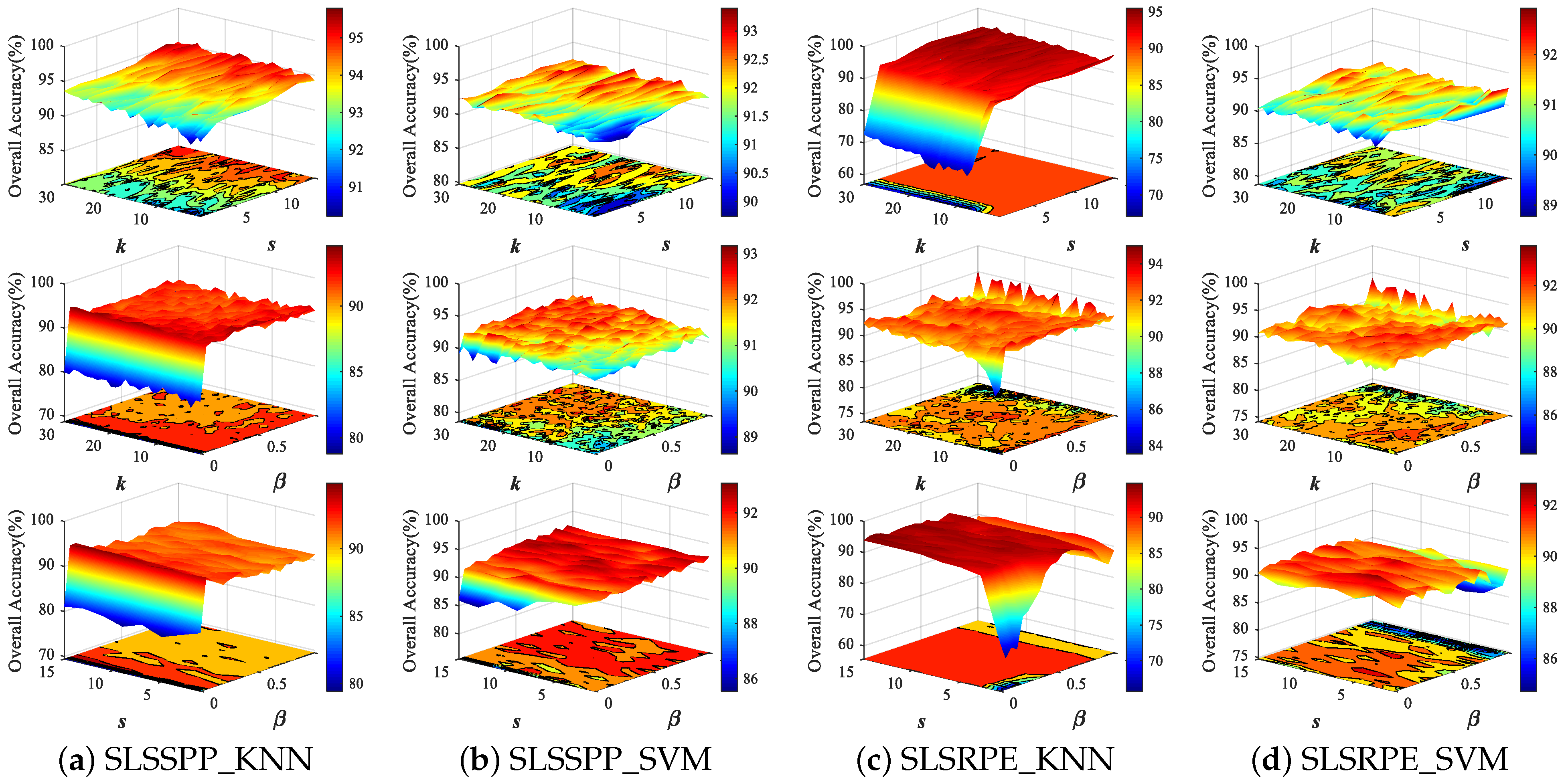
4.3. Parameters Analysis

The two proposed uSLSML methods both have three parameters: nearest neighbor number k, spatial window size s and spectral-locational trade-off parameter $\beta$. In order to analyze the influence of three parameters on the DR results, we conduct parameter tuning experiments on three HSI datasets. Thirty samples in each class are randomly selected as the training set and the remaining samples are the testing set for two classifiers. For ease of analysis, Figure 6 and Figure 7 show the classification OAs with different parameters on Indian Pines and PaviaU datasets. In experiments, the parameter values are set to: $k=\{1,2,\dots ,30\}$, $s=\{1,3,\dots ,15\}$, $\beta =\{0,0.05,0.1,\dots ,1\}$. The fixed parameters of SLSSPP and SLSRPE are set to $k=15$, $s=5$, $\beta =0.4$ on Indian Pines dataset, $k=20$, $s=3$, $\beta =0.01$ on PaviaU dataset to analyze the other two parameters.

We first analyzed the effect of SLSSPP parameters on classification. From Figure 6 and Figure 7, the classification OA increases slightly with the increase in k and s when $\beta$ is fixed, while the OA significantly increases with the increase in $\beta$ when k and s are fixed, respectively, on two datasets. In particular, the change in $\beta$ developing from nothing brings a significant improvement to the classification. This proves that the location information is quite beneficial for DR for classification. However, the OAs have not changed much as $\beta$ continues to grow, because the value of location information is much larger than that of spectral information due to the normalization of spectral bands.

For the proposed SLSRPE method, the OAs increase as s increases on two datasets when $\beta$ or k is fixed, especially for KNN classifiers, since the large spatial neighborhood is beneficial to characterize the spatial relationship between samples. This means that the spatial neighborhood added in reconstruction weights of SLSRPE is helpful for DR for classification. At the same time, the OAs are improved with the increase in $\beta$ on two datasets on account of the importance of location information to DR for classification. It is worth noting that compared with KNN, SVM has stronger robustness to parameters in view of the advantages of SVM model training.

In fact, when k is greater than 15, the influence of k on uSLSML tends to be stable. For a new HSI datum, k can be valued between 15 and 30. The setting of s depends on the smoothness of the image. If the homogeneous pixels of the HSI image are relatively clustered, s can take a larger value and vice versa. Actually, the further increase in s after increasing to 5 does not significantly improve uSLSML. Therefore, in order to ensure the low computational complexity and the effectiveness of dimension reduction, s can be set to $5\sim 15$. The value of $\beta$ is obviously influenced by the size of the image. If the image size is large, the value of $\beta$ should be small, and vice versa. $\beta$ usually ranges from 0.01 to 1. In the following experiment, the parameters of SLSSPP are set as $k=28$, $s=11$, $\beta =0.7$ for the Indian Pines dataset, $k=25$, $s=13$, $\beta =0.05$ for the PaviaU dataset, $k=26$, $s=15$, $\beta =0.03$ for the Salinas dataset. The parameters of SLSRPE are set as $k=9$, $s=9$, $\beta =1$ for the Indian Pines dataset, $k=26$, $s=15$, $\beta =0.02$ for the PaviaU dataset, and $k=14$, $s=15$, $\beta =0.03$ for the Salinas dataset.

4.4. Dimension Analysis

In order to analyze the impact of the embedding dimension d of each DR algorithm on classification performance, thirty samples from each class are randomly selected as the training set, and the rest as the test set. If the number of samples in a class is less than 60, half of the samples in this class are used as the training set. Figure 8 gives the OAs with a different embedding dimension for various DR algorithms on three datasets. The embedding dimension d is tuned from 2 to 40 with an interval of 2.

As can be seen from Figure 8, the OAs in the low-dimensional space are mostly higher than those in the raw space. This proves that DR is necessary for classification. Meanwhile, the OAs of each algorithm gradually increases with the increase in embedding dimension, because the higher-dimensional embedding features contain more discriminative information that is helpful for classification. However, as the dimension continues to grow, the OAs tends to be stable or even slightly decreased. The reason is that the discriminative information of the embedding space is gradually approaching saturation and the Hughes phenomenon occurs due to fewer training samples for classifiers. In addition, it is obvious that the classification performance of the DR algorithm fusing spatial and spectral information, LPNPE, SSRLDE [14], SSMRPE [24], SSLDP [27], SLSSPP and SLSRPE, is generally higher than that of the spectral-based algorithm, LPP [20], NPE [21] and RLDE [14], which effectively testifies that spatial information is beneficial to DR for classification. It is worth noting that compared with other DR algorithms, in this experiment, SLSSPP and SLSRPE achieve the best classification performance in almost all embedding dimensions of the three datasets, because SLSSPP and SLSRPE take full advantage of spectral-locational-spatial information in HSIs for DR. In order to ensure each algorithm achieves optimal performance, we set the embedding dimension $d=30$ on three datasets in the following experiments.

4.5. Classification Result

In practical applications, the classification accuracy of the DR algorithm is sensitive to the size of training set. To explore the classification performance of DR algorithms under different training conditions, we randomly selected $n_i$ ($n_i=5,10,20,30,40,60$) samples from each class for training, and the others for testing. If the number of samples in a class is less than $2n_i$, half of samples in this class are randomly selected for training.

Table 5. Classification OAs of the embedding features (dim = 30) of different DR algorithms on three datasets using KNN and SVM classifiers under different training conditions.

	Classifier	KNN							SVM
Dataset	${\mathit{n}}_{\mathit{i}}$	5	10	20	30	40	60	5	10	20	30	40	60
Indian	RAW	54.3	64.3	72.5	77.2	79.7	83.4	58.2	70.6	81.2	85.4	88.4	91.3
	NPE	69.4	77.3	85.2	88.3	90.0	93.0	72.6	79.9	86.3	89.9	91.9	93.7
	LPP	69.4	76.8	85.3	88.2	90.2	92.9	72.2	80.0	86.7	90.3	92.3	93.7
	RLDE	68.4	78.4	86.5	89.4	91.4	93.4	67.8	78.3	85.9	90.0	91.6	93.9
	LPNPE	77.7	85.0	92.4	95.1	95.4	96.9	80.5	87.1	92.6	94.7	96.1	96.9
	SSRLDE	78.4	83.6	88.2	91.3	93.3	95.0	78.3	82.9	88.6	91.0	92.7	95.1
	SSMRPE	72.7	81.8	88.0	90.4	92.9	95.0	73.9	81.8	88.7	91.7	93.0	94.9
	SSLDP	72.0	81.8	88.4	93.0	94.2	96.2	73.8	81.2	86.9	91.7	92.5	94.5
	SLSSPP	84.1	90.6	96.0	96.7	98.0	98.3	82.7	92.0	95.2	96.1	96.5	97.8
	SLSRPE	88.1	92.0	97.3	97.1	98.4	98.9	86.4	91.5	94.1	95.5	96.8	97.4
Pavia U	RAW	59.7	64.7	71.6	75.0	77.0	80.9	70.0	77.0	84.6	89.2	92.0	93.1
	NPE	58.2	63.7	73.4	76.7	80.8	83.8	66.5	79.6	86.8	90.2	93.3	93.9
	LPP	67.2	74.3	83.6	86.9	88.8	90.9	68.6	81.0	88.6	91.5	93.7	94.3
	RLDE	71.6	79.5	84.9	86.9	88.5	90.4	69.4	77.8	86.3	88.6	91.4	93.8
	LPNPE	61.3	71.6	77.5	81.7	84.2	86.8	66.7	80.4	88.0	90.2	92.6	93.3
	SSRLDE	78.1	84.7	89.3	91.3	93.1	94.6	69.4	78.6	86.1	89.2	90.9	93.0
	SSMRPE	82.0	86.0	90.5	93.6	94.3	95.9	74.8	82.6	88.4	91.1	92.8	95.2
	SSLDP	70.5	83.1	87.7	91.3	86.6	92.9	69.9	80.0	86.8	90.1	91.5	94.1
	SLSSPP	82.6	90.6	93.9	95.8	96.3	97.6	86.7	89.6	93.4	95.3	95.3	96.5
	SLSRPE	87.7	92.4	96.2	96.3	96.9	97.7	77.4	85.9	90.7	93.6	95.1	96.3
Salinas	RAW	83.3	86.2	88.8	89.1	90.4	91.0	86.0	88.6	90.9	92.4	93.1	94.2
	NPE	81.6	85.2	87.3	88.0	88.5	90.1	85.5	89.9	91.3	92.9	94.4	95.0
	LPP	89.2	91.1	92.8	94.0	94.8	95.2	88.4	90.8	93.1	94.1	94.7	95.6
	RLDE	88.8	90.0	92.7	94.3	94.6	95.7	84.7	86.5	89.3	90.9	91.9	92.8
	LPNPE	86.1	88.5	90.4	91.6	92.1	93.2	85.3	88.2	90.5	91.8	92.5	93.7
	SSRLDE	86.9	92.3	89.7	95.8	96.3	97.0	80.5	88.8	90.8	92.4	93.1	94.3
	SSMRPE	89.6	91.3	93.5	94.1	94.9	96.1	89.3	91.6	94.0	94.5	95.1	95.9
	SSLDP	90.6	92.8	92.8	95.1	95.6	96.0	89.5	90.0	91.9	92.4	92.7	93.5
	SLSSPP	93.5	94.7	96.7	97.1	97.7	98.3	94.6	94.4	95.7	96.1	97.0	97.1
	SLSRPE	91.4	95.9	96.1	97.0	97.3	98.1	90.2	923	93.9	94.7	95.1	96.4

shows the classification OAs of the embedding features of different DR algorithms on three datasets using KNN and SVM classifiers under different training conditions.

As shown in Table 5, for three datasets, the larger the number of training samples is, the higher the OA value is, since a large number of training samples with class labels can enable a supervised DR algorithm and classifier to obtain more discriminative information. In the comparison algorithms, the spectral-spatial algorithms, LPNPE, SSRLDE [14], SSMRPE [24], and SSLDP [27] are superior to the spectral-based algorithms, including LPP [20], NPE [21], and RLDE [14]. The supervised spectral-spatial algorithms, SSRLDE [14] and SSLDP [27], are better than the unsupervised spectral-spatial algorithms, including LPNPE [14]. These demonstrate once again that label and spatial information are advantageous to DR for classification.

As mentioned in Section 1, obtaining class labels is time-consuming, expensive, and difficult. Thus, the sensitivity of the classification performance of the DR algorithm to the number of training samples with class labels can also be used to evaluate the DR algorithm. Without doubt, we expected that the classification of a DR algorithm can achieve good performance with fewer training samples with class labels. From Table 5, it is as expected that when $n_i=5$, SLSRPE on Indian Pines and PaviaU datasets, and SLSSPP on the Salinas dataset achieve the best and satisfactory classification performance in this experiment. In addition, the proposed uSLSML achieved better classification results than other algorithms under almost all training conditions of this experiment. Because uSLSML presents a new SLSD to extract SLS information to choose the effective neighbor and constructs an SLS adjacency graph and a cluster centroid adjacency graph for SLSSPP to enhance the separability of embedded features, it also redefines the reconstruction weights for SLSRPE to mine the SLS reconstruction relationships among samples to discover the intrinsic manifold structure of HSIs.

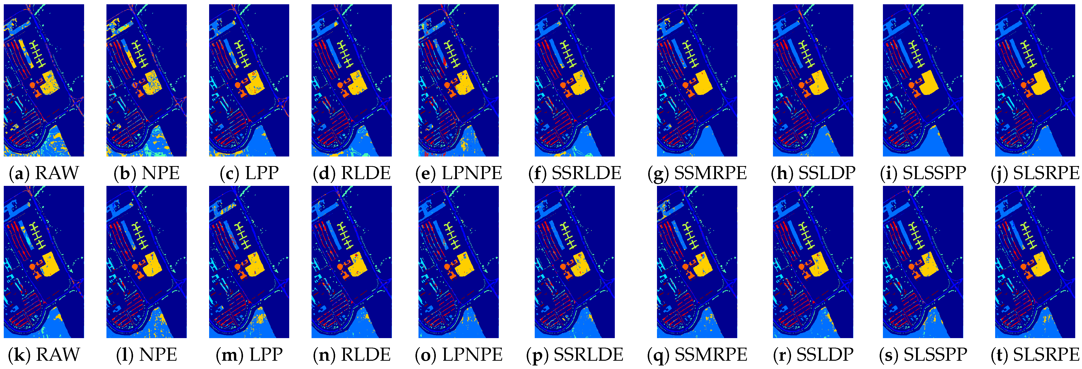
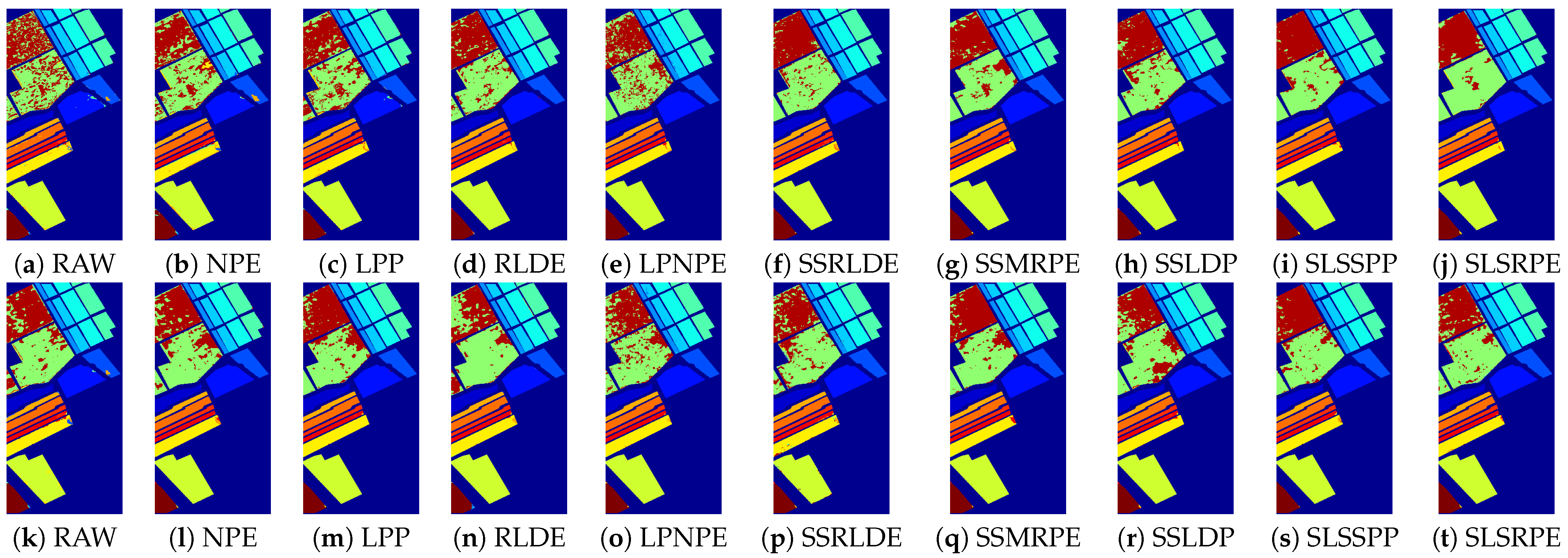
In order to explore the classification accuracy of different DR algorithms on each class, we classified the embedding features of different DR algorithms with the KNN and SVM classifier on three datasets.

Table 6. Classification accuracy of the embedding features on each class with SVM and KNN classifiers in Salinas dataset.

Class	Classifier	RAW	NPE	LPP	RLDE	LPNPE	SSRLDE	SSMRPE	SSLDP	SLSSPP	SLSRPE
C1	KNN	99.1	99.8	99.1	99.9	100	100	100	100	100	100
	SVM	99.5	99.7	99.8	100	100	100	100	100	99.6	100
C2	KNN	97.8	99.3	98.5	99.9	100	100	100	100	100	100
	SVM	99.5	100	99.8	100	100	100	100	100	100	100
C3	KNN	96.8	93.9	99.7	100	100	100	100	100	100	100
	SVM	96.8	100	100	100	100	100	100	100	100	100
C4	KNN	99.3	98.4	99.2	98.5	98.8	97.9	98.4	98.9	99.7	99.3
	SVM	99.5	98.8	99.5	98.8	98.5	96.3	98.5	99.3	99.1	99.4
C5	KNN	96.0	96.0	96.6	99.5	92.4	99.9	99.8	99.2	98.9	99.2
	SVM	96.6	99.3	99.6	97.7	96.2	99.8	98.9	99.2	99.0	99.7
C6	KNN	99.3	99.2	99.7	99.8	100	100	100	100	100	99.9
	SVM	99.8	99.9	99.8	98.7	99.7	99.6	100	100	100	99.5
C7	KNN	99.6	99.1	98.6	99.6	100	99.9	99.9	100	100	99.9
	SVM	100	99.4	99.9	99.6	99.9	99.9	99.8	99.9	100	100
C8	KNN	69.6	74.9	72.2	85.0	76.6	89.5	84.8	85.6	86.5	93.6
	SVM	83.5	81.3	80.2	86.0	79.6	81.9	76.2	84.6	90.8	87.8
C9	KNN	98.2	97.6	98.3	100	99.9	100	100	100	100	100
	SVM	97.1	100	100	100	100	98.0	100	100	100	99.9
C10	KNN	91.7	84.6	95.6	97.8	95.8	95.4	97.8	97.8	99.1	97.0
	SVM	91.8	95.0	99.4	96.0	97.4	93.8	96.8	96.2	99.0	97.7
C11	KNN	97.4	97.1	97.9	100	99.7	99.8	100	100	99.6	100
	SVM	94.0	99.8	100	99.3	100	99.6	98.9	100	99.8	99.1
C12	KNN	98.1	100	100	100	99.9	100	100	100	100	100
	SVM	99.9	99.9	100	100	100	99.9	99.9	100	100	100
C13	KNN	99.7	98.4	98.6	99.9	99.5	100	99.9	100	99.9	100
	SVM	99.8	99.1	99.9	99.5	98.4	99.7	99.7	99.3	99.1	98.1
C14	KNN	93.8	93.1	95.1	97.6	97.3	91.5	95.9	98.9	98.6	99.1
	SVM	92.4	99.3	97.9	99.3	97.6	95.5	96.5	99.8	98.7	99.6
C15	KNN	74.0	74.1	80.1	89.5	77.7	94.8	92.7	89.5	92.2	91.0
	SVM	83.0	83.8	91.3	66.0	76.4	80.3	76.2	91.9	90.5	85.4
C16	KNN	97.6	97.2	99.2	98.4	99.4	99.2	98.6	99.5	100	98.6
	SVM	98.4	98.6	99.5	97.3	99.0	98.6	98.0	99.0	99.0	99.3
OA	KNN	88.5	89.1	90.4	95.1	91.3	96.6	95.5	95.3	95.9	97.1
	SVM	92.7	93.4	94.5	91.8	92.0	92.7	91.3	95.3	96.6	95.2
AA	KNN	94.2	93.9	95.5	97.8	96.1	98.0	98.0	98.1	98.4	98.6
	SVM	95.7	97.1	97.9	96.1	96.4	96.4	96.2	98.1	98.4	97.8
$\kappa$	KNN	87.2	87.9	89.3	94.6	90.4	96.2	95.0	94.8	95.5	96.8
	SVM	91.9	92.7	93.9	90.9	91.1	91.8	90.4	94.8	96.2	94.6

,

Table 7. Classification accuracy of the embedding features for each class with SVM and KNN classifiers in Indian Pines dataset.

Class	Classifier	RAW	NPE	LPP	RLDE	LPNPE	SSRLDE	SSMRPE	SSLDP	SLSSPP	SLSRPE
C1	KNN	95.7	100	100	100	100	100	100	100	100	100
	SVM	100	100	100	100	100	100	100	100	100	100
C2	KNN	66.5	67.0	78.9	85.8	83.9	91.6	78.8	93.4	94.8	96.3
	SVM	85.8	89.2	93.6	91.1	94.3	93.3	88.6	94.8	95.4	94.5
C3	KNN	76.3	73.1	82.3	91.0	96.8	92.8	89.4	92.1	96.0	98.6
	SVM	87.3	93.4	92.1	89.6	97.4	86.8	94.9	87.8	97.1	98.5
C4	KNN	88.9	96.1	98.1	99.0	99.0	97.6	97.1	100	99.5	99.5
	SVM	90.8	97.1	97.1	99.5	99.0	100	94.2	100	98.1	99.5
C5	KNN	89.8	90.7	95.4	99.1	93.8	99.8	93.2	96.0	99.3	96.0
	SVM	94.5	96.0	94.7	97.8	98.2	98.5	94.7	96.5	98.1	95.4
C6	KNN	96.7	97.7	97.9	99.1	99.9	98.7	99.4	99.7	100	100
	SVM	99.3	100	100	98.0	100	99.6	100	99.1	99.1	99.6
C7	KNN	100	100	100	100	100	100	100	100	100	100
	SVM	100	100	100	100	100	100	100	100	100	100
C8	KNN	93.8	94.0	96.9	99.6	100	98.9	97.8	100	100	100
	SVM	93.8	100	100	99.3	100	98.0	100	100	99.6	100
C9	KNN	100	100	100	100	100	100	100	100	100	100
	SVM	100	100	100	100	100	100	100	100	100	100
C10	KNN	83.0	82.6	91.3	90.6	95.3	91.8	90.8	92.6	97.1	94.4
	SVM	80.3	93.1	88.6	89.0	96.6	92.0	91.9	87.9	96.6	89.2
C11	KNN	65.1	70.6	75.5	87.1	91.2	89.3	85.3	93.0	94.4	97.5
	SVM	73.2	67.8	83.3	82.6	80.6	85.2	74.4	87.3	91.5	93.2
C12	KNN	67.7	75.7	72.6	92.5	95.9	93.6	92.4	93.3	98.9	92.7
	SVM	82.4	96.4	94.5	95.7	98.6	96.3	96.4	93.3	94.1	97.2
C13	KNN	99.4	97.7	98.3	98.9	99.4	98.3	99.4	99.4	100	100
	SVM	97.7	98.9	100	99.4	99.4	99.4	99.4	99.4	100	100
C14	KNN	91.7	95.0	90.4	95.1	99.8	93.8	98.7	96.1	99.7	98.7
	SVM	93.3	93.9	93.8	96.4	97.5	97.5	95.6	96.6	98.5	98.4
C15	KNN	82.9	81.5	93.3	99.2	97.8	99.4	88.2	100	99.7	100
	SVM	91.0	95.5	98.9	99.2	99.7	96.3	97.5	99.7	99.7	99.4
C16	KNN	100	100	100	100	100	100	100	100	100	100
	SVM	100	100	100	100	100	100	100	100	100	100
OA	KNN	78.3	80.5	85.1	91.9	94.2	93.4	90.0	94.9	97.1	97.4
	SVM	85.4	87.9	91.8	91.5	93.3	92.7	89.6	92.9	96.0	95.7
AA	KNN	87.3	88.9	91.9	96.1	97.1	96.6	94.4	97.2	98.7	98.4
	SVM	91.8	95.1	96.0	96.1	97.6	96.4	95.5	96.4	98.1	97.8
$\kappa$	KNN	75.5	77.9	83.1	90.8	93.3	92.4	88.7	94.2	96.7	97.0
	SVM	83.4	86.3	90.6	90.3	92.4	91.6	88.2	91.9	95.4	95.1

and

Table 8. Classification accuracy of the embedding features on each class with SVM and KNN classifiers in the Pavia University dataset.

Class	Classifier	RAW	NPE	LPP	RLDE	LPNPE	SSRLDE	SSMRPE	SSLDP	SLSSPP	SLSRPE
C1	KNN	73.4	74.2	83.3	90.8	70.3	92.7	84.9	88.0	92.8	96.0
	SVM	87.0	94.5	94.4	91.5	90.7	91.9	90.8	91.4	88.7	91.4
C2	KNN	67.2	61.1	86.9	88.2	80.4	91.1	96.1	95.3	97.2	98.1
	SVM	89.6	88.4	86.0	95.6	94.8	95.6	94.4	92.0	97.1	94.8
C3	KNN	72.1	75.1	88.9	74.2	81.5	79.4	80.4	89.1	88.9	95.7
	SVM	85.5	81.6	90.0	80.3	86.9	76.9	75.2	89.5	91.0	88.5
C4	KNN	86.1	87.5	94.0	93.9	87.5	95.0	92.0	94.1	90.0	96.5
	SVM	94.2	93.3	94.3	93.7	94.2	93.6	96.1	93.3	94.0	92.8
C5	KNN	99.8	99.7	100	100	100	100	100	99.8	100	100
	SVM	99.6	100	100	99.9	100	99.9	99.9	100	100	100
C6	KNN	82.1	75.1	90.7	92.2	92.3	95.1	97.7	99.4	99.8	99.9
	SVM	94.9	94.9	94.0	92.0	94.9	90.9	93.8	92.8	97.1	98.0
C7	KNN	85.8	69.5	93.6	95.1	97.2	97.8	99.2	98.8	99.7	96.2
	SVM	96.7	98.5	95.9	97.4	98.5	98.2	96.8	99.2	99.4	97.4
C8	KNN	75.7	77.9	79.4	90.9	63.1	93.4	87.5	87.7	89.4	83.4
	SVM	86.8	83.3	82.1	69.7	71.8	75.8	85.4	85.6	89.2	73.4
C9	KNN	99.8	99.8	98.8	99.8	100	99.9	100	99.9	99.9	99.9
	SVM	99.8	99.9	99.9	100	99.7	99.9	99.8	100	99.8	100
OA	KNN	74.5	71.1	87.6	89.9	80.8	92.4	93.1	93.9	95.4	96.5
	SVM	90.5	90.6	89.8	91.7	92.2	92.0	92.5	92.1	94.9	92.7
AA	KNN	82.4	80.0	90.6	91.7	85.8	93.8	93.1	94.7	95.3	96.2
	SVM	92.7	92.7	93.0	91.1	92.4	91.4	92.5	93.8	95.2	92.9
$\kappa$	KNN	67.9	63.9	83.9	86.8	75.5	90.1	90.8	92.0	94.0	95.4
	SVM	87.6	87.7	86.7	89.1	89.7	89.5	90.2	89.6	93.2	90.4

listed the classification accuracy of each class, OA, AA, and Kappa coefficient. The visualized classification maps of different approaches on three datasets are displayed in Figure 9, Figure 10 and Figure 11.

From Table 6, Table 7 and Table 8, the spatial-spectral combined methods are completely superior to spectral-based methods and supervised spatial-spectral algorithms slightly outperform unsupervised spatial-spectral algorithms. This means that compared with the label information, the spatial information is more conducive to improving the representation of embedded features in this experiment. SLSRPE and SSMRPE [24] are two improved versions of NPE [21], both of which are dedicated to maintaining the local manifold structure of the data. Table 6, Table 7 and Table 8 show that their improvement is effective, and SLSRPE is more outstanding than SSMRPE [24]. The proposed SLSD can find more neighbor samples from the same class than the SSCD of the SSMRPE [24], and more importantly, SLSRPE adds the SLS information to the reconstruction weights to reveal the intrinsic manifold structure of HSIs. This experiment also testifies that SLSSPP is far superior to LPP, which is attributed to the proposed SLSD and the new DR model with an SLS adjacency graph and a cluster centroid adjacency graph.

It is worth mentioning that SLSRPE and SLSSPP are even more outstanding than the supervised spectral-spatial algorithms, SSRLDE [14] and SSLDP [27], which are two graph-based methods. For supervised graph-based methods, the supervised information is usually placed in the adjacency graph. The above implicitly proves the excellence of the extracted SLS information stored in the adjacency graph of uSLSML.

Specifically, SLSSPP achieves the best classification results in 9 and 10 classes on the Indian Pines dataset, 5 and 3 classes on the PaviaU dataset, 8 and 10 classes on the Salinas dataset for KNN and SVM classifiers, respectively. SLSRPE achieves the best classification results in 9 and 7 classes on the Indian Pines dataset, 4 and 3 classes on the PaviaU dataset, and 9 and 6 classes on the Salinas dataset for KNN and SVM classifiers, respectively. From the numerical value of OA, SLSSPP and SLSRPE are more suitable for the KNN classifier because these two algorithms are based on distance. In general, SLSSPP and SLSRPE are more outstanding than other comparison algorithms in this experiment, due to the full exploration of the spectral-locational-spatial information of HSIs.

According to the classification maps in Figure 9, Figure 10 and Figure 11, SLSSPP and SLSRPE produce smoother classification maps and less misclassification pixels compared with other DR methods, especially in the classes that Corn-notill, Soybean-mintill for the Indian Pines dataset, Asphalt, Meadows, Gravel for the Pavia University dataset, Grapes-untrained, Vinyard-untrained for the Salinas dataset. These maps illustrate that the comprehensive exploration of SLS information ignored by other comparison algorithms is very helpful for the low-dimensional representation of HSIs and it is absorbed by SLSSPP and SLSRPE.

5. Concluding Remarks

In this paper, we propose two unsupervised DR algorithms, SLSSPP and SLSRPE, to learn the low-dimensional embeddings for HSI classification based on the spectral-locational-spatial information and manifold learning theory. A wSL datum is generated to facilitate the extraction of SLS information. A new SLSD is designed to search the proper nearest neighbors most probably belonging to the class of target samples. Then, SLSSPP constructs a DR model with an SLS adjacency graph based on SLSD and a cluster centroid adjacency graph based on wSL data to preserve SLS structure in HSIs, which compresses the nearest neighbor distance and expands the distance among clustering centroids to enhance the separability of embedding features. SLSRPE constructs an adjacency graph based on the redefined reconstruction weights with SLS information, which maintains the intrinsic manifold structure to extract the discriminant projection. As a result, two uSLSML methods can extract two discriminative low-dimensional features which can effectively improve the classification performance.

Extensive experiments on the Indian Pines, PaviaU and Salinas datasets demonstrated that the points we proposed are effective and the proposed uSLSML algorithms perform much better than some state-of-the-art DR methods in classification. Compared with LPP, the average improvements of OA are about 3.50%, 2.44%, 2.05% by the cluster centroid adjacency graph, 8.24%, 6.55%, 3.09% by SLSD, and 9.04%, 8.67%, 3.26% by SLSSPP on three datasets, while compared with NPE, the improvements are about 5.31%, 12.25%, and 5.05% by redefined reconstruction weights with SLS information, 4.38%, 3.75%, 1.75% by SLSD, 9.66%, 13.27%, 5.72% by SLSRPE.

This work just considers the neighbor samples and ignores the target samples in exploring the local spatial neighborhood information. Thus, our future work will focus on solving this problem while reducing the computational complexity.