Abstract
In this paper, additional reference height errors, caused by the penetration depth and Signal to Noise Ratio (SNR) decorrelation in desert regions in L-band spaceborne bistatic interferemetric SAR, will introduce significant errors in nowadays baseline calibration method based on distributed target and consequent DEM products. To quantify these two errrors, this paper takes the TwinSAR-L mission as an example, gives an introduction of TwinSAR-L, outlines the theoretical baseline accuracy requirements that need to be satisfied in the TwinSAR-L mission and addresses the additional reference height errors caused by the penetration depth and SNR decorrelation in desert regions in general by taking the TwinSAR-L mission as an example. Based on ALOS-2 data from a dry desert region in the east of Xing Jiang, this paper quantitatively analyzes these additional reference height errors. The results show that the additional reference height errors resulted from the penetration depth and the SNR decorrelation are 1.295 m and 1.39 m, respectively, which would even cause 6.4 mm and 8.6 mm baseline calibration errors. These errors would seriously degrade the baseline calibration accuracy and the consequent DEM product quality. Therefore, our analysis is of great significance not only for baseline calibration, but also for high-quality DEM’s generation, accuracy assessment and geophysical parameters’ quantitative inversion and application.
1. Introduction
In the last decade, an increasing amount of attention has been paid to the bistatic space-borne Interferometric Synthetic Aperture Radar (InSAR), which is nowadays a well-recognized and effective instrument for deriving digital elevation models (DEMs). DEMs are widely used in many scientific and commercial fields, such as hydrology, glaciology, forestry, geology, etc., which need up to date and accurate information about the surface and topography of earth [1,2,3]. A well-known example of bistatic space-borne InSAR is the TanDEM-X system, which can generate a high-quality global DEM with excellent absolute height error below 2 m (linear 90% error) [4,5]. Compared with the X-band InSAR system, an L-band system has more advantages because of its longer wavelength, strong penetration ability and high temporal coherence over vegetated areas. These advantages make it possible not only to generate high-precision digital terrain model with less influence of vegetation, but also better to realize the global measurement of forest height and related biomass with PolInSAR and multi-baseline tomography techniques [6,7,8]. It can also fulfill the measurement of deformations and motions on the Earth with accuracy down to centimeters or even millimeters using repeat-pass interferometry [9,10,11]. Therefore, many countries, such as Germany, Japan, and China, are vigorously developing L-band space-borne SAR. For example, European Space Agency (ESA) has proposed the Europe L-band (ROSE-L) mission [12], this mission responds to a request from the land monitoring and emergency management services. It will be applied to land cover mapping, soil moisture measurement, forest type/forest cover (in support to biomass estimation), maritime surveillance, food security and precision farming, and natural and anthropogenic hazards. The NASA-ISRO Synthetic Aperture Radar (NISAR) Mission is a multi-disciplinary radar mission cooperated by the National Aeronautics and Space Administration (NASA) and the Indian Space Research Organization (ISRO). It aims to carry out comprehensive measurements to better comprehend the reasons and consequences of land surface changes, which is the first dual-frequency SAR mission in the world (L band and S band), and will be launched in December 2021 [13].
TwinSAR-L mission which belongs to the medium- and long-term development plan for China’s civil space infrastructure will be launched in 2021 [14]. The TwinSAR-L is an innovative space-borne bistatic SAR mission, also called LuTan-1 (LT-1), with two L-band SARs flying in a much longer across-track baseline (4–6 km), compared with TanDEM-X [15,16]. The main goal of the mission is to achieve highly accurate terrain and deformation measurements with the requirement of a 5 m absolute height accuracy for flat to moderate terrain on a grid of 3 m by 3 m. To meet the criteria concerning the DEM accuracy, precise knowledge of the interferometric SAR system parameters, especially of the baseline, is essential. The baseline has to be determined down to a reasonable range in order to minimize the possibility of an InSAR-derived height error. The baseline measurement accuracy is mainly affected by the following three factors: the relative orbit position measured by GPS and Satellite Laser Ranging (SLR), the spacecraft attitude measured by Star Trackers, and the location of the SAR antenna phase center [15,17].
In TanDEM-X mission, a novel method based on a distributed target DEM was proposed to calibrate baseline errors in the plane perpendicular to the flight direction . As a result, the baseline product can achieve the 2 mm absolute accuracy requirement [15]. The primary motivation of this paper is to investigate whether this calibrated method can be applied in other L-band bistatic space-borne InSAR systems such as TwinSAR-L.
However, the successful use of the distributed target calibration method in the TanDEM-X mission implies two assumptions: (1) The penetration is minimal, and the ideal InSAR-derived DEM is physically the same as or nearly equal to the laser altimeter, so the reference DEM provided by the distributed target (laser altimeter) can be used directly; (2) The SNR of the distributed target (typically a sandy area [15] is high enough, so the interferometric phase errors caused by SNR decorrelation can be ignored. However, for L-band SAR such as ALOS, ALOS-2 and TwinSAR-L, these two assumptions have been validated and may not be true. Based on the samples of Bir Safsaf sand in the south central desert of Egypt, paper [18] found that the penetration depth of L-band was 1.5–2.0 m, C-band was 0.2–0.5 m, and X-band was 0.1–0.3 m. Similar work has also been conducted in paper [19], which found that the retrieved L-band InSAR DEM is always 1–2 m lower than that of the C-band Space Shuttle Radar terrain mission (SRTM) DEM in the sandy area. It is obvious that the L band’s penetration depth can’t be ignored compared with C- or X-band SAR. In addition, the SNR decorrelation of X band SAR has also been analyzed by many scholars. For example, paper [20] found that if X-band spaceborne bistatic SAR surveys adopt steeper incidence angles, the SNR (up to 15 dB) and coherence (usually higher than 0.8) can be significantly improved. Thus, the SNR decorrelation errors can be ignored. However, the SNR decorrelation of L band SAR has been rarely mentioned, which cannot be neglected through our simulation results. For the acquisition, processing, precision analysis of L-band data, the characteristics of band, ground object penetration effect and SNR should be fully considered, otherwise it will lead to wrong results. In addition, the selection criteria for the baseline calibration of the distributed target as the reference DEM in the L band has rarely been mentioned and discussed. In this paper, the reference height errors caused by the distributed target itself, especially the penetration depth in general, are analyzed by taking the TwinSAR mission as an example, and simulations and experiments explain the irrationality of these two assumptions.
This paper is organized as follows. Section 2 reviews the baseline calibration method based the distributed target DEM, introduces additional errors when using the baseline calibration method based on the distributed target DEM in TwinSAR-L, and proposes the estimation methods of additional reference height errors caused by penetration depth and SNR decorrelation. Then, combined with ALOS-2 data and parameters of the TwinSAR-L system, these estimation methods are used in Section 3 to derive the additional reference height error and baseline error results. Finally, discussions about the penetration depth estimating method’s accuracy and the baseline calibration method for TwinSAR-L, conclusion about the additional reference height errors’ influence for low-frequency spaceborne formation InSAR system are provided in Section 4 and Section 5, respectively.
2. Materials and Methods
2.1. Baseline Calibration Method Based on the Distributed Target DEM
To enhance the quality of the DEM, several baseline estimation (or calibration) methods have been proposed [21,22], which can be divided into three categories: (1) The orbit method [21,23], the basis of which is the direct computation of the two satellite tracks through satellite ephemeris data; and (2) the frequency method [24], which relies on the frequency features of the interferogram. This method is based on the fact that the baseline parameter is a function of the interferometric fringe frequency in a flat terrain, so this method only works well in a flat area; (3) the ground control points (GCPs)-based method, which is used to calibrate the baseline based on a point target or distributed target with a known height [25,26].
In TanDEM-X mission, a novel method based on a distributed target DEM was proposed to calibrate baseline errors in the plane which is perpendicular to the flight direction . With a known accurate reference DEM (ICESat laser altimeter with absolute accuracy better than 0.5 m), the baseline error parallel to the line of sight (LOS) can be calculated through Equation (2) by using the height differences between the reference DEM and a given RawDEM (InSAR-derived DEM before baseline calibration), then combining at least two different , can be obtained.
Baseline errors of spaceborne formation InSAR system can be decomposed into three components: radial, cross-track, and along-track errors. The along-track errors can be effectively resolved by co-registration and regarded as uncritical [15,27]. The radial and cross-track errors can be converted into baseline errors: in the line of sight and perpendicular to the line of sight . According to paper [15], the baseline bias vector is expressed by:
where and are the real variables, and is a unitary vector which is perpendicular to the line-of-sight.
According to [15,28], has the most significant influence on the DEM height error . The relationship is expressed as:
where is the height of ambiguity, which is equivalent to the height of phase change of a fringe, and is given by Equation (3):
where r and are the slant range distance and the incident angle of an appropriately selected reference point (e.g., at midswath), respectively.
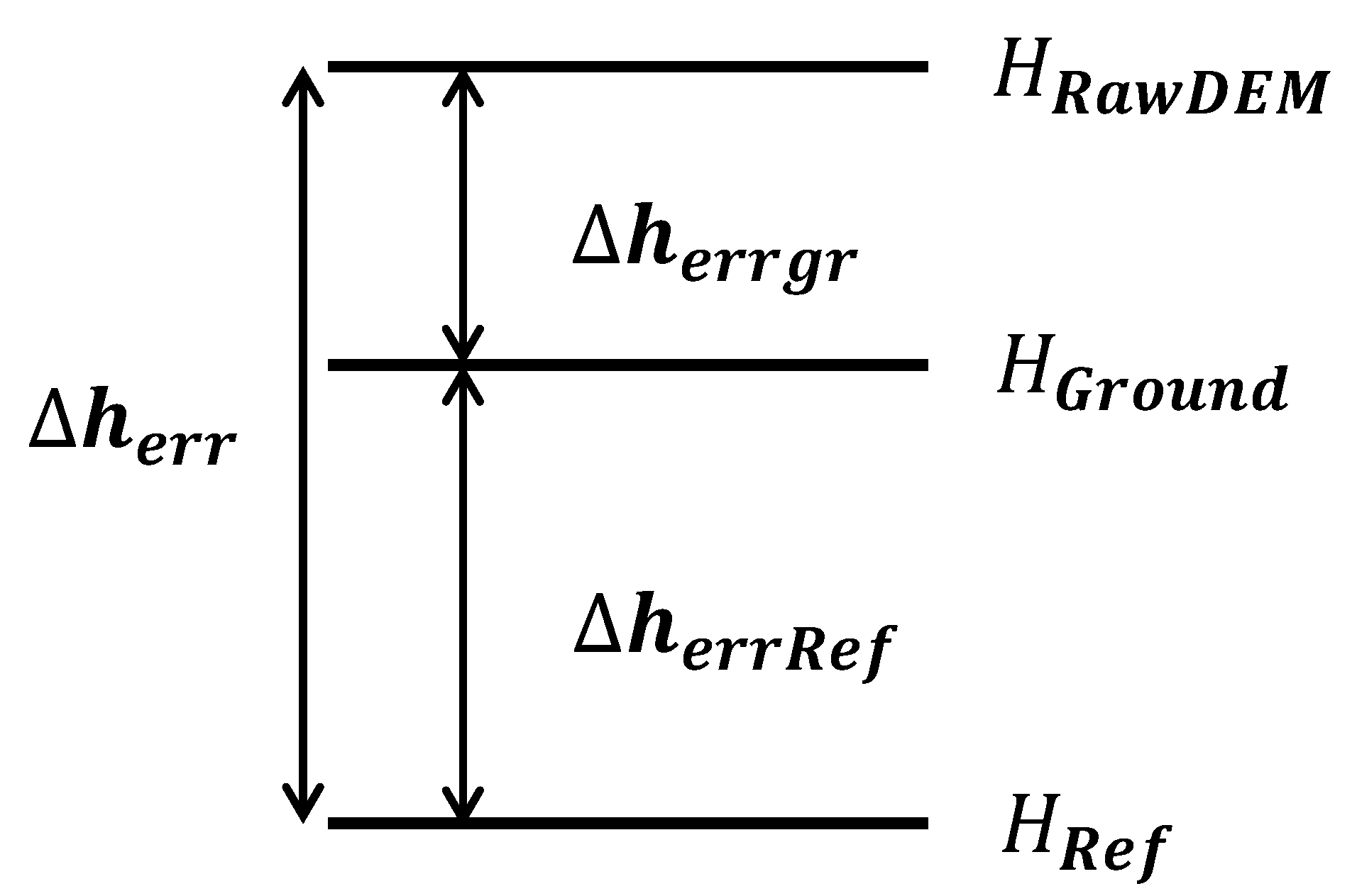
Applying , the height differences between (the DEM derived by the InSAR system), and (the reference DEM derived by ICEsat) to Equation (2), and can be calculated. The composition of is shown in Figure 1, and can be divided into two parts: (1) The effective height error (), which refers to the height bias between (the real height of the ground) and ; (2) The error of the reference height (), i.e., between and [15].
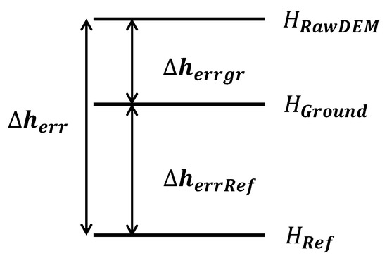
Figure 1.
Composition of a height error [15].
In the TwinSAR-L mission, the composition of has significant differences. As shown in Table 1, the in L band not only contains the measurement errors of the reference height (i.e., , the error from the altimeter itself, such as the ICEsat), but also the additional reference height errors and , which are caused by the penetration bias, and the SNR decorrelation, respectively.

Table 1.
The composition of in the X and L band.
As stated in paper [15], the height error can also be given by:
where is the phase offset corresponding to a baseline error in line of sight and it is considered to be constant [15,27].
If the reference is correct with , the is constant. On the other hand, the reference has the following errors: , and , which can be expressed as:
Then, Equation (6) can be derived as:
The reference height errors derived by measurement , the penetration depth , and the SNR decorrelation could induce a dependence on the height of ambiguity, which causes an unstable . Therefore, the chosen standard for the reference DEM and estimation of the penetration bias and SNR decorrelation plays significant roles in the baseline calibration process, and the estimation methods for these two additional reference height error sources (penetration depth and backscattering coefficient) will be given in Section 2.2 and Section 2.3, respectively.
2.2. Additional Reference Height Error of L-Band
The penetration of radar to dry sand and soil varies with the wavelength and angle of the incident signal and the electrical properties of the material, which largely depends on the soil moisture content [22,29]. Compared with X-band signal, L-band has a stronger capability to penetrate the subsurface down to several meters in arid sand [30,31]. This leads to the additional height error contributing to an unstable baseline bias. In order to achieve higher baseline calibration accuracy, how to estimate the penetration depth is vitally important.
In recent years, there are a few studies on the penetrability of SAR of microwaves, mainly divided into the following three categories: (1) methods which use Ulaby’s penetration depth model based on soil moisture, roughness, and soil composition [31,32]; (2) methods based on the height differences between dual-frequency InSAR data [33,34]; (3) methods based on the inversion of scattering model [35]. The application scope of the first method is limited by large number of unknown parameters as the input of the model; the second method has strict requirements on observation conditions and observation area, and requires a shorter observation interval between two bands of InSAR to avoid temporal changes in physical properties of the observation area. At the same time, the dual-frequency InSAR is required to be: one low-frequency InSAR that can penetrate the desert significantly, and the other high-frequency with negligible penetration depth. In addition, this method requires the height measurement accuracy of the dual-frequency InSAR to be high enough to obtain high-precision penetration depth estimation. This approach is more of theoretical significance, and difficult to be applied in practice; the third method is based on SAR signal’s scattering and refraction process when it penetrates the desert layer. In order to describe the scattering and refraction process of InSAR signal penetrating the infinite volume, Dall [35] proposed a coherent scattering model to estimate the penetration depth, which has been well verified in the snow-, ice and forest covered area [36]. Guanxin Liu [37,38,39] extended the scattering model to inversion of desert layer penetration depth from InSAR data, but its inversion highly depends on the coherence of InSAR data.
In this paper, based on the first and third methods, combined with the backscattering coefficient information of the actual SAR data, the soil surface roughness and moisture content of the study area are inverted firstly, then the dielectric constants are inverted by using the relationship between the dielectric constant and the soil moisture content established in the literature [40], and finally the penetration depth of the study area is calculated.
According to Ulaby’s theoretical model, the penetration depth may be defined as the depth , at which the electromagnetic wave’s power falls to , where e represents the base of natural logarithm [38,41], i.e.,
where is the real part of the dielectric constant and is the imaginary part of the dielectric constant, is the wavelength of the incident wave, and for most natural materials, except water, < 0.1.
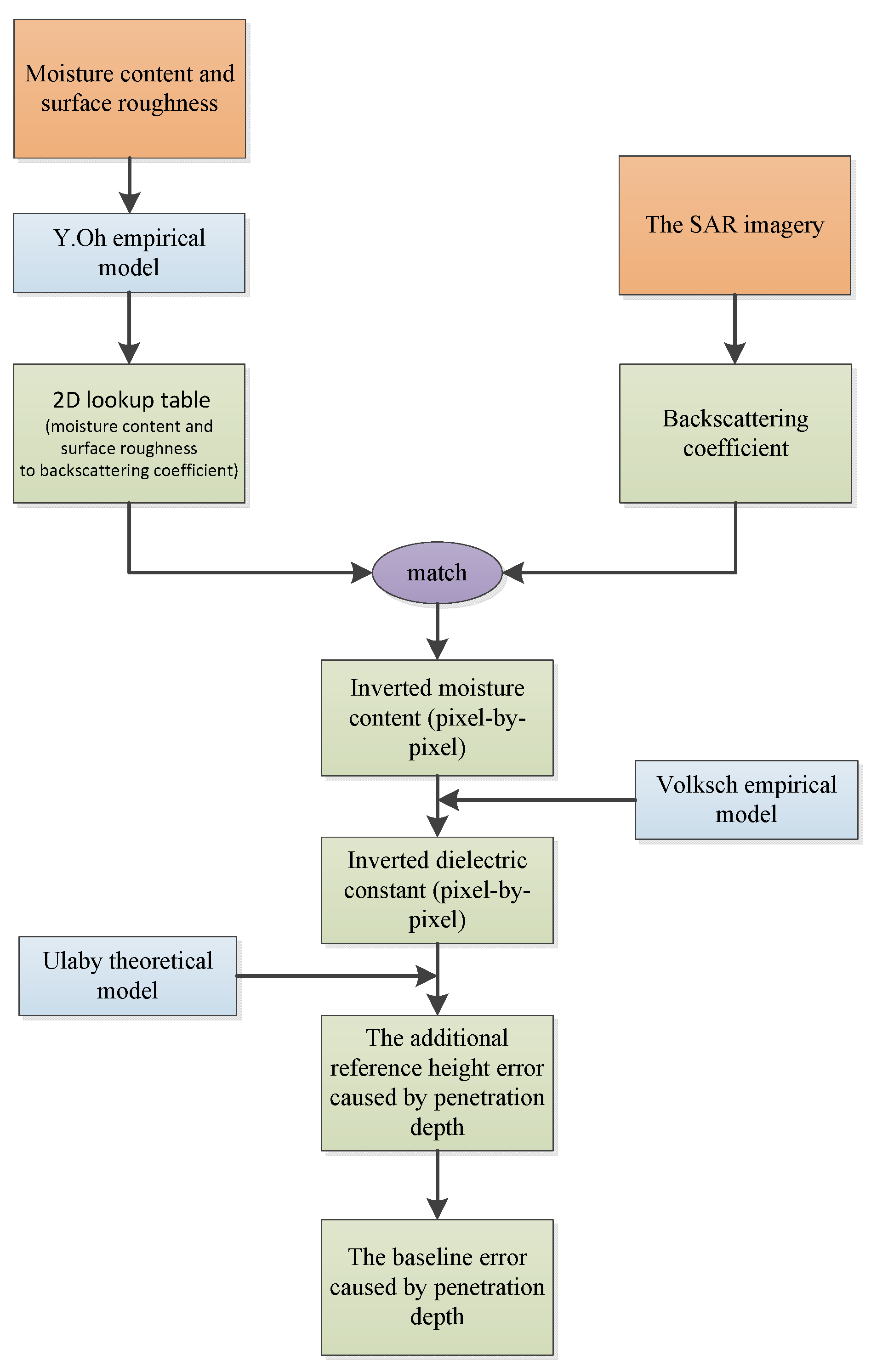
To estimate the penetration depth, it is necessary to obtain the study area’s dielectric constant first, which is directly related to the SAR image’s backscattering coefficient. As shown in Figure 2, the empirical model proposed by Y.Oh. [42] is used to retrieve the dielectric constant, which has high accuracy for bare soil surface with different roughness and humidity. Generally speaking, the root-mean-square (rms) height (surface roughness) ranges from 0.2 cm to 2.0 cm [43,44], and the soil moisture content is 0.01–0.4% (by volume) [45], which are reasonable values ranges for dry sand. With the given ranges of the soil surface roughness and moisture content, the HH-polarized backscattering coefficient can be acquired through Equation (9), which establishes a 2-D lookup table.
where the incidence angle, is the soil moisture content, (is the wavenumber), and s is the rms height.
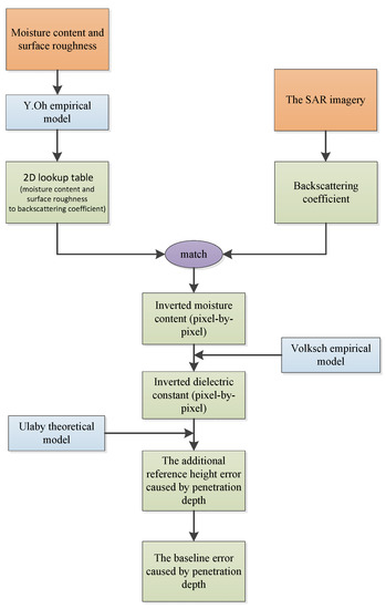
Figure 2.
Workflow designed to estimate additional reference height error .
After obtaining the , according to the matching condition of minimum absolute value difference between the and from the SAR imagery, as described in Equation (10), we can find the soil water content corresponding to each pixel from the 2-D lookup table, which can be considered as the actual value of the study area’s soil moisture content.
After obtaining the soil moisture content, based on the empirical model established by Volksch [40], as shown by Equation (11), we can invert the dielectric constant pixel-by-pixel, then take the dielectric constant into Ulaby’s model, the additional reference height error can be inverted.
2.3. Additional Reference Height Error of L-Band
For distributed target, the backscattering coefficient can be simply defined as the radar-cross section (RCS) per unit area [41,46]. According to paper [20], it is obvious that radar backscattering coeffiecient mainly depends upon the dielectric properties of the material, terrain, incidence frequency, and varies with the geometry of the looks. Assuming other conditions are the same, the backscattering coefficient in the L-band is lower than that in the X-band, which leads to a worse SNR. The worse SNR causes interferometric phase errors, which bring in a non-ignorable height error .
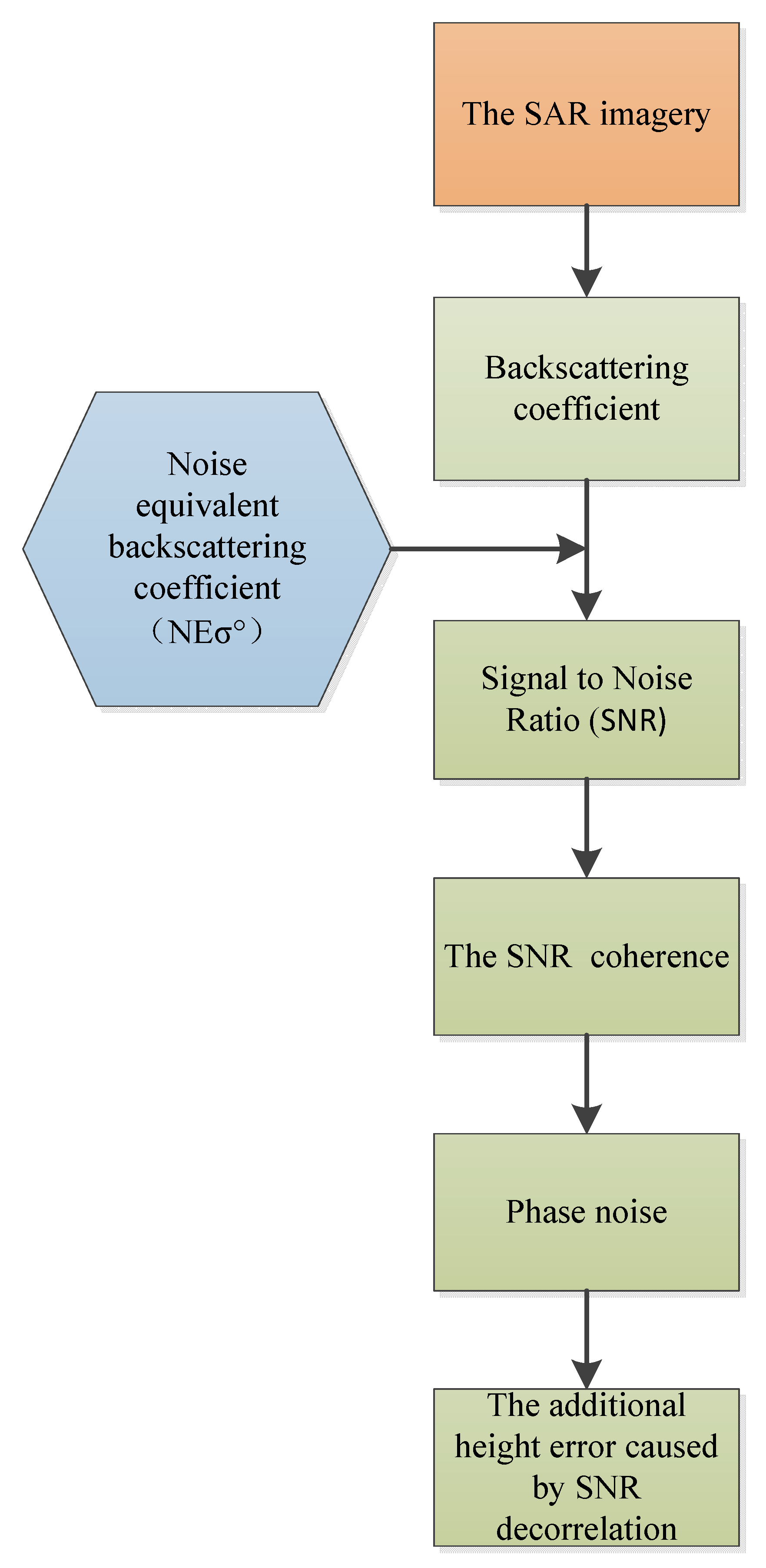
As shown in Figure 3, in order to estimate , we first need to get the backscattering coefficient of the study area, and then calculate the SNR with the noise equivalent backscattering coefficient () of TwinSAR-L system, and deduce the phase noise caused by SNR decorrelation, and finally the reference height error caused by SNR decorrelation is calculated.
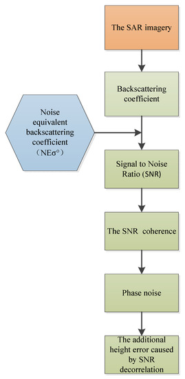
Figure 3.
Workflow designed to estimate additional reference height error .
As shown in paper [47], the SNR of the distributed target can be expressed as:
Using to present the noise equivalent backscattering coefficient, the equation reduces to:
where can be expressed as:
where R is the distance between the target and radar; K is the Boltzmann constant, and J/K; c is the speed of light; is the transmitted signal bandwidth; is the system losses; T is the temperature of the receiver; is the receiver noise figure; G is the antenna gain; V is the platform velocity; is the local beam incidence angle; is the SAR wavelength; is the average transmitting power of the SAR. Taking the parameters of the TwinSAR-L system into Equation (14), the value of can be calculated and is better than −28 dB. The SNR coherence is a function of SNR, which can be expressed as:
is one of the major contributors to the interferometric phase noise, which affects the measurement uncertainty of the InSAR-derived height, because noise will interrupt the phase measurement. Interferometric phase noise caused by can be expressed as the below equation:
where N is the number of looks, and in the simulation of next section, the value of N is 24.
Finally, the additional height error attributed to SNR decorrelation can be expressed as:
3. Results and Analysis
As mentioned in Section 2.1, one main factor of the distributed target baseline calibration is the accuracy of the reference DEM. However, the special properties of L band have an essential impact on the precision of the reference DEM. We have described the two additional error sources and , as well as their theoretical analysis and simulation methods in Section 2.2 and Section 2.3, the simulation result of the two additional errors in the TwinSAR-L mission are analyzed, and the system simulation parameters are shown in Table 2.
Table 2.
Parameters of the TwinSAR-L system.
To achieve its primary target of deriving a high-quality DEM, the TwinSAR-L system adopts a single transmitter dual receiver interferometry mode: one satellite transmits, and both satellites receive the signal echoes effectively. The interferometry mode parameters are shown in Table 3.
Table 3.
Parameters of the interferometry mode.
As TwinSAR-L has not been launched, it is impossible to obtain its actual data, so the two additional errors are simulated with the Advanced Land Observing Satellite-2 (ALOS-2) Phased Array-type L-Band Synthetic Aperture Radar (PALSAR) data obtained under HH polarization configuration over a desert area in Hami, Xinjiang Province of China on 5 March 2020.
3.1. Test Site and Data Sets
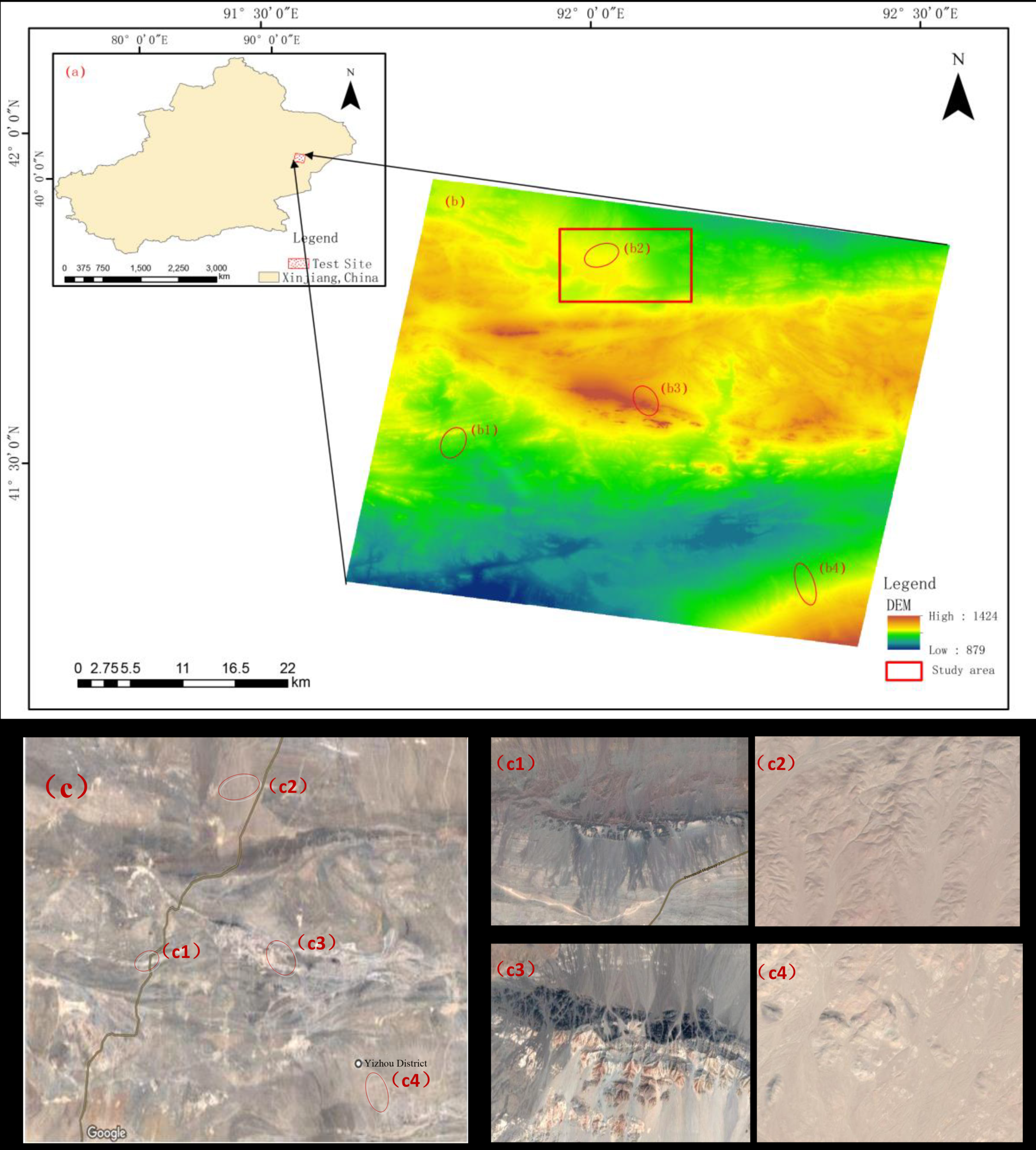
Hami is located in the east of Xinjiang, China, at a longitude of E to E and latitude of N to N, covering an area of more than 130,000 km. The area belongs to dry-warm temperate continental climate, with low rainfall, high evaporation, big temperature difference, strong winds. As a result, the soil in this area is very dry and most of it is covered with desert. The selected test site of TwinSAR-L acquried by ALOS-2 is located in Hami as Figure 4a,b show, the exposed rocks and rocks covered by shallow sand are shown in Figure 4(b1,b3), and the uniform sand is shown in Figure 4(b2,b4). To consider the instrument induced errors of reference DEM, we choose the relatively flat terrain as the study area, which is marked by the red rectangle in Figure 4b. This region’s slope ranges from to . In order to see the geomorphic features of the study area more clearly, Figure 4(c,c1–c4), optical images showing the test site were downloaded from Google Earth Engine (GEE, https://earthengine.google.org, accessed on 15 March 2021). Furthermore, Figure 4(b,b1–b4) correspond to Figure 4(c,c1–c4), respectively. The acquired ALOS-2 data was in the HH polarization over a desert area in Hami, Xinjiang Province of China. The center incident angle was , the SAR imagery’s original resolution is azimuth × range = 10 m × 10 m.
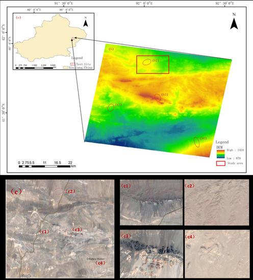
Figure 4.
Location of the test site and study area. (a) Xingjiang, China. (b) Test site’s DEM. (b1,b3) shows exposed rocks and rocks covered by shallow sand, (b2,b4) are covered by uniform sand. (c) Test site’s optical image from Google earth. (c1–c4) show the geomorphic features correspond to (b1–b4), respectively.
3.2. Additional Error Reference Height of L-Band
Figure 5a shows the SAR amplitude map of the test site. The darker parts are related to the regions covered by uniform sand, and the brighter parts correspond to the area covered by exposed rocks. Figure 5b shows the backscattering coefficient map of the test site.
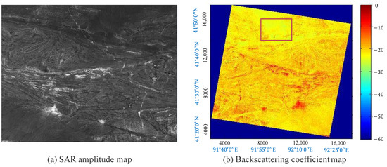
Figure 5.
(a) The attitude map of the test site. (b) backscattering coefficient map of the test site.
In order to quantitatively analyze the SNR decorrelation effect, the backscattering coefficient of the uniform sand is selected as the study area, marked by the red rectangle in Figure 5, with an average value of −23.22 dB (The subsequent quantitative analysis objects in this paper are all this region).
According to the estimation workflow of penetration depth in Figure 2, a 2-D lookup table of the soil surface roughness and moisture content is established, and ALOS-2 data is used to determine the soil moisture content with the minimum Z value in Equation (10), that is, the value closest to the actual soil moisture content of the test site. The soil moisture content’s image in the test site is shown in Figure 6, the values of inverted soil moisture content in the area corresponding to the red rectangle range between and , the average value is (by volume), which is in line with the normal range of soil moisture content in Hami desert.

Figure 6.
The soil moisture content map of the test site.
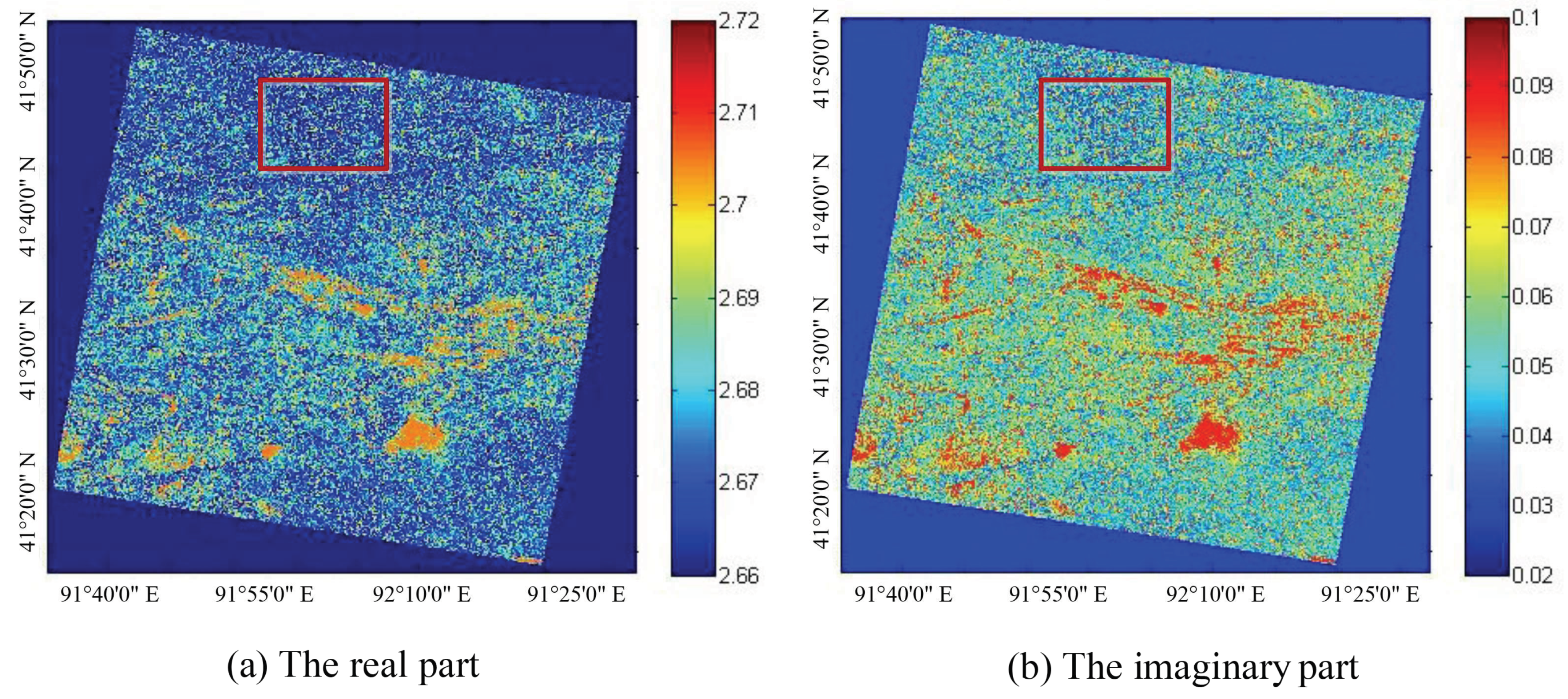
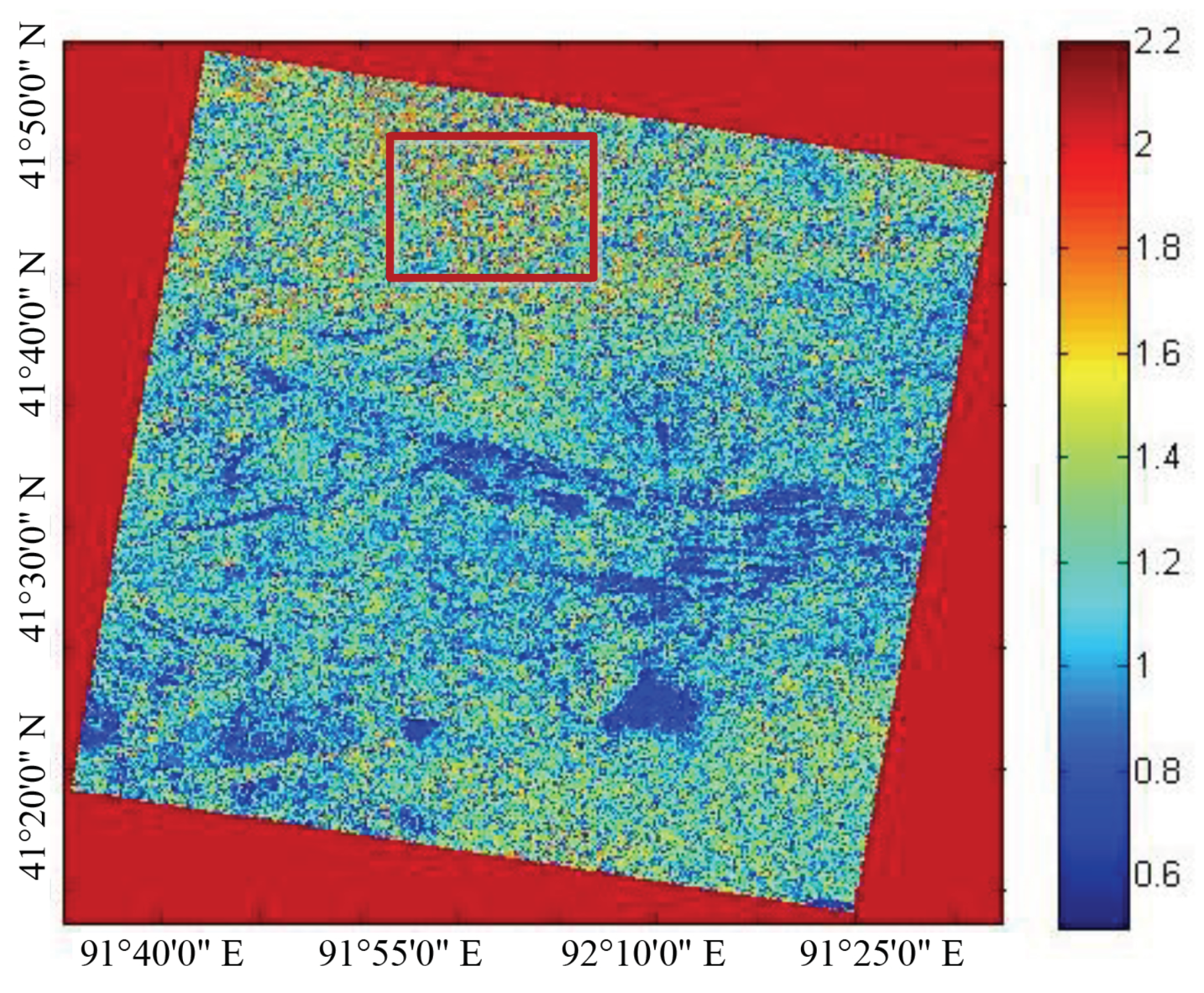
Based on Volksch empirical model, the inverted dielectric constant map is shown in Figure 7. Obviously, the dielectric values (both the real part and imaginary part) of the rocks are relatively large, so the SAR signal is difficult to penetrate; the dielectric values of the uniform sand region are relatively small, and the SAR signal is easy to penetrate. The average value of the real part and imaginary part of the uniform sand covered area marked by red rectangle is 2.675 and 0.052, respectively, which is consistent with the existing studies [29,40].
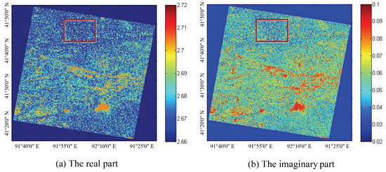
Figure 7.
The dielectric constant map of the test site. (a) The real part. (b) The imaginary part.
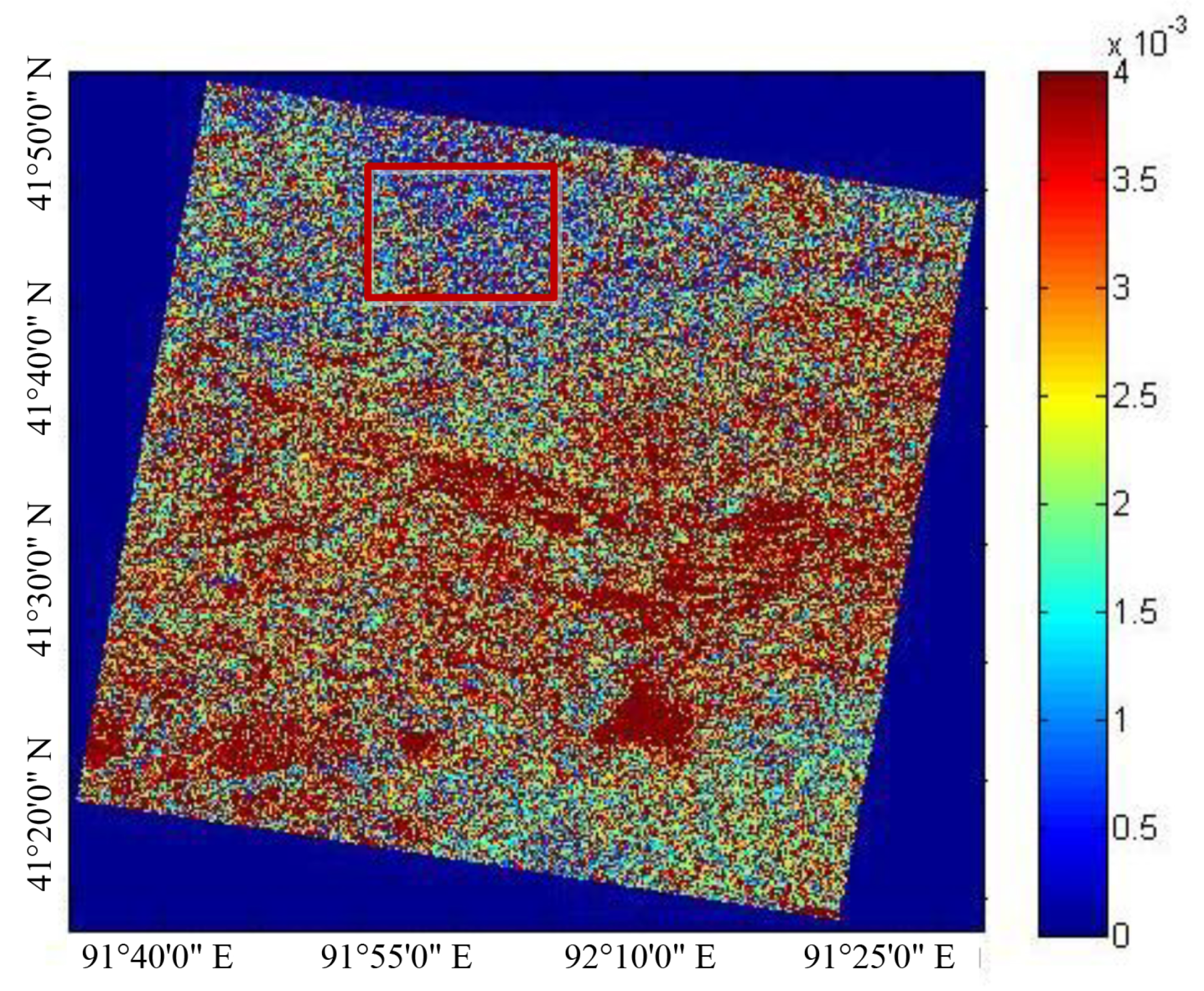
The calculated dielectric constant is then used to invert the penetration depth, i.e., of L band, which is shown in Figure 8. It can be found that the corresponding penetration depth values of the L-band are mainly between 0 and 1m in the area covered by rocks; for the sand region, the corresponding penetration depth are mainly in the range of 1 to 2 m, and the average value in the red rectangle region is 1.295 m.

Figure 8.
The Penetration depth estimation map of the test site.
3.3. Additional Error Reference Height of L-Band
According to the estimation workflow of in Figure 3, combined with ALOS-2 data and of TwinSAR-L system, the SNR cohenrence map of the test site is shown in Figure 9. The results show that the SNR coherence values are greater than 0.7 in the rock covered area, some part values are even greater than 0.9; for the sand region, the values of coherence are between 0.4 and 0.7, most of which are greater than 0.5.
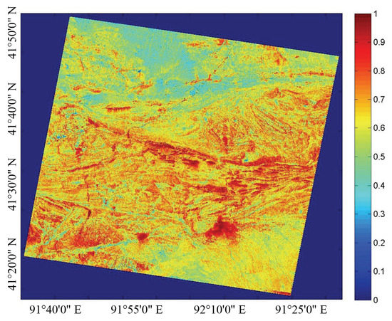
Figure 9.
The SNR coherence map of the test site.
The calculated SNR coherence is then used to invert the reference height error caused by SNR decorrelation, as shown in Figure 10. The result shows that values of L-band SAR signal in sandy region are around 1 m to 2 m; for the area covered by rock, the corresponding values are smaller, which ranges from 0 to 1 m. Corresponding, the average of the uniform sand area, which is shown in the red rectangle in Figure 10, is 1.39 m.
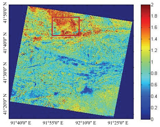
Figure 10.
The reference height error caused by SNR decorrelation.
4. Discussion
4.1. Penetration Depth Estimation Accuracy
Although the estimation method proposed in this paper can get the reasonable penetration depth of SAR signal in desert area, based on Equations (8) and (11), but it is obvious that the accuracy of the estimation method mainly depends on the inversion of the soil moisture content. Therefore, to ensure a good inversion result, the selection range of the soil moisture content is of great importance.
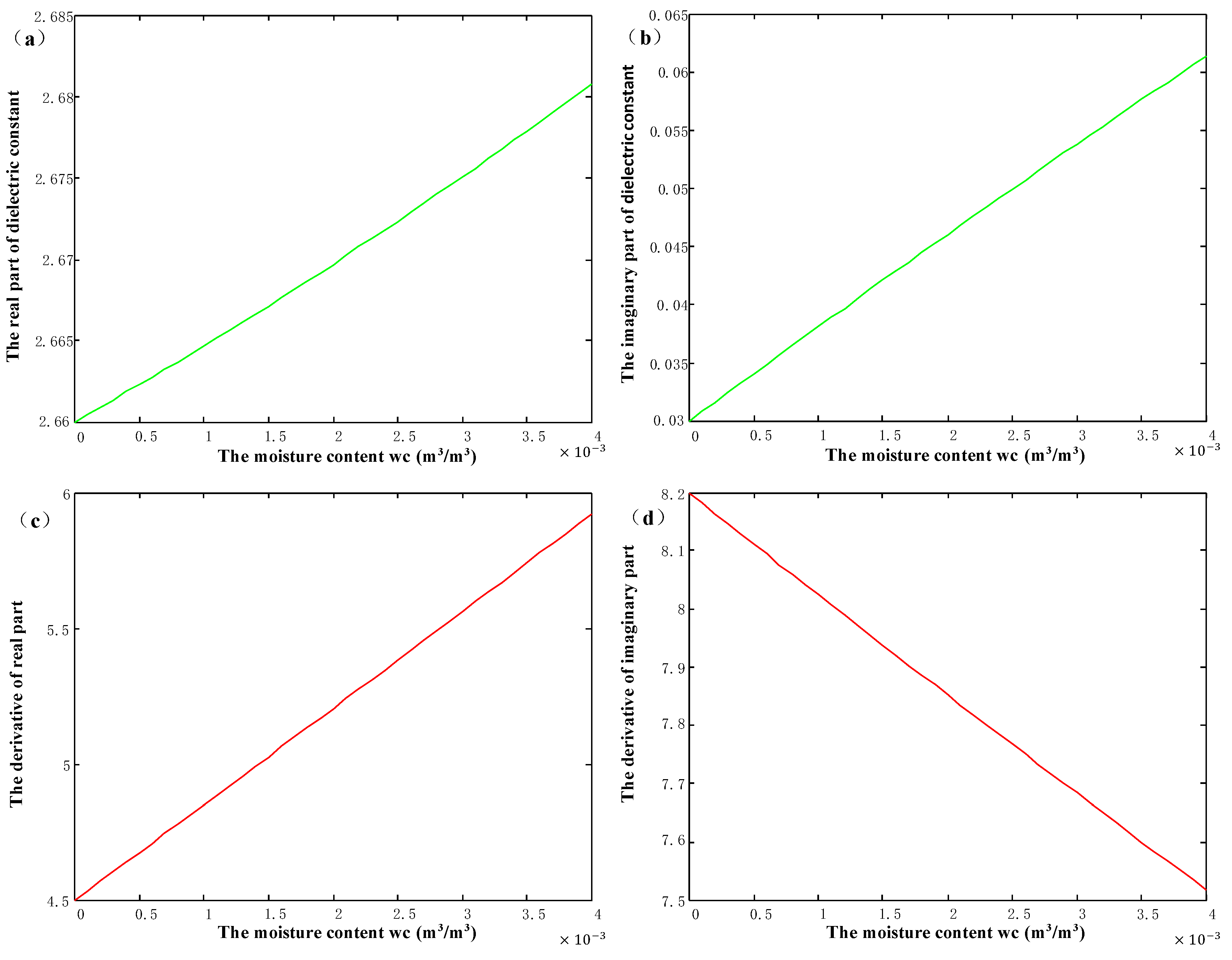
According to Equation (11), dielectric constant (both the real and imaginary part) is expressed as a function of the soil moisture content , and the derivative with respect to can be used to describe the sensitivity of the dielectric constant to the changes of as follows:
Figure 11 shows the dielectric constant values (both the real and imaginary part) and their derivatives changing with different values of . It is apparent that the values of dielectric constant increase with the increasing . The real part of the dielectric constant is essentially constant, all values being between 2.66 and 2.68, although the corresponding derivative increases from 4.5 to 5.92 while varies from 0 to 0.4%, and. The imaginary part of dielectric constant changes greatly with soil moisture content, all values being between 0.03 and 0.0614 and the corresponding derivative decreases from 8.2 to 7.52 while ranges from 0 to 0.4%.
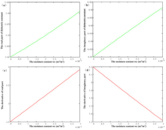
Figure 11.
(a) The real part, (b) the imaginary part of dielectric constant. (c) The real part, (d) the imaginary part of derivative with respect to .
According to Equations (8) and (11), penetration depth can be expressed as a function of the soil moisture content , and the derivative with respect to can be used to describe the sensitivity of the penetration depth to the changes of as follows:
where
where A, B and C have no physical meanings, only used to express Equation (19) concisely.
Figure 12 shows the penetration depth values of L band SAR signal in desert area and their derivatives changing with different values of . With the increase of , the penetration depth of L band decreases, for example penetration depth while ; while . The result that the penetration depth of L-band SAR in dry sand area is around 1–2 m is consistent with the existing data [29,40,48] and our simulation result.
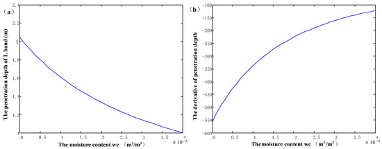
Figure 12.
(a) The penetration depth of L band. (b) The derivative with respect to .
As stated in Section 3.2, the inverted soil moisture content of the study area ranges between 0.01% and 0.36%, the derivative of penetration depth ranges from −526.6 to −135.6, as shown in Figure 12b. It is assumed that the soil moisture content inversion by the method proposed in this paper has an absolute error of 0.05%, the estimation error of penetration depth ranges from 0.07 m to 0.26 m.
By assuming a minimum penetration for the L band in desert area equals 1.035 m , the Baseline length of B equals 4 km and baselines corresponding to a height of ambiguity of = 38 m–51 m (i.e., km for and km for ), we can simply deduce that this part of reference height error will cause a baseline calibration error of 4.8 mm to 6.4 mm according to Equation (7).
4.2. The Baseline Calibration Method for TwinSAR-L
The average value of the reference height error caused by the backscattering properties in the study area is 1.39 m. By assuming the same baseline and height of ambiguity parameters as in Section 4.1, we can simply deduce that this part of the reference height error will cause a baseline calibration error of 6.4 mm to 8.6 mm. As shown in Table 2, the requirement for baseline calibration is 6mm, which cannot be satisfied due to the two reference height errors, and a miscalibration of the baseline will further lead to a deterioration of the DEM product accuracy generated by the InSAR, instead of improving it. The quality of DEM product will affect the accuracy of global base map, large scale deformation and the monitoring of ocean, earthquake, Landslides, cryosphere. Therefore, these two issues, which have not been well concerned in C- or X-band, must be paid enough attention to in L band, not only for single-pass bistatic space-borne but also repeat-pass space-borne InSARs. In our future work, we will obtain the backscattering coefficient of the test site through field measured data or radiometric calibrated space-borne L-band SAR images in order to calculate the reference height error more accurately.
According to the error analysis results, an improved baseline calibration method based on distributed targets should be developed for the L-band spaceborne bistatic InSAR, such as TwinSAR-L mission. In the future work, we try to deal with these two errors in two ways: (1) Continuing to use the distributed target calibration method but compensating for the error penetration error in the generation of the penetration depth correction datasets in conjunction with the penetration depth of the dependence of the dielectric constant, incident angle, wavelength, and appropriate features of the dielectric constant; (2) The point target is adopted to replace the distributed target, which is a traditional intuitive method. The penetration problem of natural ground objects can be avoided by using artificial point targets (corner reflectors or active radar calibrators). The error introduced by the signal-to-noise ratio can be reduced by point targets with a large RCS. Using point targets instead of distributed targets can reduce these two additional reference height errors introduced in this paper and effectively improve the accuracy of the DEM products generated by TwinSAR-L. However, the distribution of the number of point targets is limited, the volume and weight of the L-band 3 m corner reflector are large, so it is very difficult to layout, and the calibration frequency is limited by the revisit period of the InSAR system on the calibration field. By using the combination of distributed target and point target baseline calibration methods, the reference elevation can be generated by the wide range of distributed targets, and then the reference elevation error of distributed targets can be corrected by using high-precision point targets.
5. Conclusions
This paper points out the potential problems associated with using the distributed target baseline calibration method in L band space-borne InSAR applications. The principles of generating additional reference height errors, and , and the methods of quantitatively analyzing these two errors are employed. From the results and analysis, we can conclude that the average values of and are 1.295 m and 1.39 m of dry sand area in the study area for TwinSAR-L, respectively. Corresponding, the baseline calibration error caused by these two errors even reach 6.4 mm and 8.6 mm, which cannot meet the 6 mm requirements of the TwinSAR-L mission. The inaccurate baseline will further affect the quality of the DEM product and the quantification of the changes in the geosphere, biosphere, hydrosphere, and cryosphere. In this context, our analysis is of great significance for research on the baseline calibration method, calibration site design, and final DEM accuracy of L-band single-pass (bistatic space-borne) and repeat-pass space-borne InSARs. The significance of this paper is to point out that the penetration and SNR factors should be well considered in L-band InSAR system calibration and applications, especially for dry areas. In addition, it will have reference value and guidance significance for some potential new research and application in L-band InSAR, such as subsurface DEM generation, quantitative inversion of geophysical parameters (soil moisture, roughness, etc.)
Author Contributions
J.H. played the leading role in preparing this paper. Y.Q. performed the simulations and analyzed the data. Y.W. contributed to the structure and revision of this paper and provided insightful comments and suggestions. S.D. provided valuable suggestions and revised the manuscript. All authors have read and agreed to the published version of the manuscript.
Funding
This research was funded by the National Natural Science Foundation of China (No. 61771453).
Conflicts of Interest
The authors declare no conflict of interest.
References
- Rossi, C.; Minet, C.; Fritz, T.; Eineder, M.; Bamler, R. Temporal monitoring of subglacial volcanoes with TanDEM-X Application to the 2014C2015 eruption within the Brearbunga volcanic system, Iceland. Remote Sens. Environ. 2016, 181, 186–197. [Google Scholar] [CrossRef] [Green Version]
- Zebker, H.A.; Farr, T.G. Mapping the world’s topography using radar interferometry: The TOPSAT mission. Proc. IEEE 1994, 82, 1774–1786. [Google Scholar] [CrossRef] [Green Version]
- Moreira, A.; Krieger, G.; Hajnsek, I.; Hounam, D.; Werner, M.; Riegger, S.; Settelmeyer, E. TanDEM-X: A TerraSAR-X add-on satellite for single-pass SAR interferometry. In Proceedings of the 2004 IEEE International Geoscience and Remote Sensing Symposium, IGARSS 2004, Anchorage, AK, USA, 20–24 September 2004; pp. 1000–1003. [Google Scholar]
- Wessel, B.; Huber, M.; Wohlfart, C.; Marschalk, U.; Kosmann, D.; Roth, A. Accuracy assessment of the global TanDEM-X Digital Elevation Model with GPS data—ScienceDirect. ISPRS J. Photogramm. Remote Sens. 2018, 139, 171–182. [Google Scholar] [CrossRef]
- Brutigam, B.; Martone, M.; Rizzoli, P.; Gonzalez, C.; Zink, M. Quality Assessment of the TanDEM-X Global Digital Elevation Model. In Proceedings of the International Symposium on Remote Sensing of Environment (ISRSE), Berlin, Germany, 11–15 May 2015. [Google Scholar]
- Lee, S.K.; Kugler, F.; Papathanassiou, K.; Hajnsek, I. First Pol-InSAR Forest Height Inversion by means of L-band F-SAR Data. In Proceedings of the ESA POLinSAR2013 Workshop, Frascati, Italy, 28 January–1 February 2013. [Google Scholar]
- Hajnsek, I.; Kugler, F.; Lee, S.K.; Papathanassiou, K.P. Tropical-Forest-Parameter Estimation by Means of Pol-InSAR: The INDREX-II Campaign. IEEE Trans. Geosci. Remote Sens. 2009, 47, 481–493. [Google Scholar] [CrossRef] [Green Version]
- Tebaldini, S.; Rocca, F. Multibaseline Polarimetric SAR Tomography of a Boreal Forest at P- and L-Bands. IEEE Trans. Geosci. Remote Sens. 2012, 50, 232–246. [Google Scholar] [CrossRef]
- Moreira, A.; Krieger, G.; Hajnsek, I.; Papathanassiou, K.; Younis, M.; Lopez-Dekker, P.; Huber, S.; Villano, M.; Pardini, M.; Eineder, M.; et al. Tandem-L: A Highly Innovative Bistatic SAR Mission for Global Observation of Dynamic Processes on the Earth’s Surface. IEEE Geosci. Remote Sens. Mag. 2015, 3, 8–23. [Google Scholar] [CrossRef]
- Liu, X.; Zhao, C.; Zhang, Q.; Lu, Z.; Li, Z. Deformation of the Baige Landslide, Tibet, China, Revealed Through the Integration of Cross-Platform ALOS/PALSAR-1 and ALOS/PALSAR-2 SAR Observations. Geophys. Res. Lett. 2020, 47, e2019GL086142. [Google Scholar] [CrossRef] [Green Version]
- Doke, R.; Kikugawa, G.; Itadera, K. Very Local Subsidence Near the Hot Spring Region in Hakone Volcano, Japan, Inferred from InSAR Time Series Analysis of ALOS/PALSAR Data. Remote Sens. 2020, 12, 2842. [Google Scholar] [CrossRef]
- Pierdicca, N.; Davidson, M.; Chini, M.; Dierking, W.; Djavidnia, S.; Haarpaintner, J.; Hajduch, G.; Laurin, G.V. The Copernicus L-band SAR mission ROSE-L (Radar Observing System for Europe) (Conference Presentation). In Proceedings of the Active and Passive Microwave Remote Sensing for Environmental Monitoring III, Strasbourg, France, 11–12 September 2019. [Google Scholar]
- Rosen, P.A.; Agram, P.S.; Lavalle, M.; Cohen, J.; Buckley, S.; Kumar, R.; Misraray, A.; Ramanujam, V.; Agarwal, K.M. The Nasa-Isro SAR Mission Science Data Products and Processing Workflows. In Proceedings of the Agu Fall Meeting, New Orleans, LA, USA, 11–15 December 2017. [Google Scholar]
- Li, C.; Zhang, H.; Deng, Y.; Wang, R.; Liu, K.; Liu, D.; Jin, G.; Zhang, Y. Focusing the L-Band Spaceborne Bistatic SAR Mission Data Using a Modified RD Algorithm. IEEE Trans. Geosci. Remote Sens. 2020, 58, 294–306. [Google Scholar] [CrossRef]
- Antony, J.M.W.; Gonzalez, J.H.; Schwerdt, M.; Bachmann, M.; Krieger, G.; Zink, M. Results of the TanDEM-X Baseline Calibration. IEEE J. Sel. Top. Appl. Earth Obs. Remote. Sens. 2013, 6, 1495–1501. [Google Scholar] [CrossRef]
- Pinheiro, M.; Reigber, A.; Moreira, A. Large-baseline InSAR for precise topographic mapping: A framework for TanDEM-X large-baseline data. Adv. Radio Sci. 2017, 15, 231–241. [Google Scholar] [CrossRef] [Green Version]
- Hueso Gonzalez, J.; Bachmann, M.; Krieger, G.; Fiedler, H. Development of the TanDEM-X Calibration Concept: Analysis of Systematic Errors. IEEE Trans. Geosci. Remote Sens. 2010, 48, 716–726. [Google Scholar] [CrossRef] [Green Version]
- Schaber, G.G.; Mccauley, J.F.; Breed, C.S. The use of multifrequency and polarimetric SIR-C/X-SAR data in geologic studies of Bir Safsaf, Egypt. Remote Sens. Environ. 1997, 59, 337–363. [Google Scholar] [CrossRef]
- Fischer, G.; Papathanassiou, K.; Hajnsek, I. Modeling and Compensation of the Penetration Bias in InSAR DEMs of Ice Sheets at Different Frequencies. IEEE J. Sel. Top. Appl. Earth Obs. Remote Sens. 2020, 13, 2698–2707. [Google Scholar] [CrossRef]
- Martone, M.; Bräutigam, B.; Krieger, G. Decorrelation effects in bistatic TanDEM-X data. In Proceedings of the 2012 IEEE International Geoscience and Remote Sensing Symposium, Munich, Germany, 22–27 July 2012. [Google Scholar]
- Ren, K.; Prinet, V.; Shi, X.; Wang, F. Comparison of satellite baseline estimation methods for interferometry applications. In Proceedings of the IGARSS ’03, Geoscience and Remote Sensing Symposium, Toulouse, France, 21–25 July 2003. [Google Scholar]
- Zhang, K.; Ng, H.M.; Li, X.; Chang, H.C.; Rizos, C. A new approach to improve the accuracy of baseline estimation for spaceborne radar interferometry. In Proceedings of the 2009 IEEE International Geoscience and Remote Sensing Symposium, Cape Town, South Africa, 12–17 July 2009. [Google Scholar]
- Krieger, G.; Fiedler, H.; Mittermayer, J.; Papathanassiou, K.; Moreira, A. Analysis of multistatic configurations for spaceborne SAR interferometry. IEE Proc. Radar Sonar Navig. 2003, 150, 87–96. [Google Scholar] [CrossRef] [Green Version]
- Chen, R.; Xu, S.J.; Zhang, P. Estimation of InSAR baseline based on the Frequency Shift Theory. In Proceedings of the 2006 CIE International Conference on Radar, Shanghai, China, 16–19 October 2006. [Google Scholar]
- Mapelli, D.; Guarnieri, A.; Giudici, D. Generation and Calibration of High-Resolution DEM From Single-Baseline Spaceborne Interferometry: The “Split-Swath” Approach. IEEE Trans. Geosci. Remote Sens. 2014, 52, 4858–4867. [Google Scholar] [CrossRef]
- Zhang, X.L.; Huang, S.J.; Wang, J.G. Approaches to estimating terrain height and baseline for interferometric SAR. Electron. Lett. 1998, 34, 2428–2429. [Google Scholar] [CrossRef]
- Krieger, G.; Moreira, A.; Fiedler, H.; Hajnsek, I.; Werner, M.; Younis, M.; Zink, M. TanDEM-X: A Satellite Formation for High-Resolution SAR Interferometry. IEEE Trans. Geosci. Remote. Sens. 2007, 45, 3317–3341. [Google Scholar] [CrossRef] [Green Version]
- Schwerdt, M.; Schrank, D.; Bachmann, M.; Gonzalez, J.H.; Antony, J. Calibration of the TerraSAR-X and the TanDEM-X Satellite for the TerraSAR-X Mission. In Proceedings of the European Conference on Synthetic Aperture Radar, Nuremberg, Germany, 23–26 April 2012. [Google Scholar]
- Stephen, H.; Long, D.G. Microwave backscatter modeling of Erg surfaces in the Sahara desert. IEEE Trans. Geosci. Remote Sens. 2005, 43, 238–247. [Google Scholar] [CrossRef] [Green Version]
- Engman, E.T.; Chauhan, N. Status of microwave soil moisture measurements with remote sensing. Remote Sens. Environ. 1995, 51, 189–198. [Google Scholar] [CrossRef]
- Schaber, G.G.; Breed, C.S. The Importance of SAR Wavelength in Penetrating Blow Sand in Northern Arizona. Remote Sens. Environ. 1999, 69, 87–104. [Google Scholar] [CrossRef]
- Matzler, C. Microwave permittivity of dry sand. IEEE Trans. Geosci. Remote Sens. 1998, 36, 317–319. [Google Scholar] [CrossRef]
- Xiong, S.; Jan-Peter, M.; Gang, L. The Application of ALOS/PALSAR InSAR to Measure Subsurface Penetration Depths in Deserts. Remote Sens. 2017, 9, 638. [Google Scholar] [CrossRef] [Green Version]
- Rui, W.; Cheng, H.; Tao, Z.; Teng, L.; Ke, Y. Subsurface height measurement using InSAR technique in sand-covered arid areas. In Proceedings of the Geoscience & Remote Sensing Symposium, Quebec City, QC, Canada, 13–18 July 2014. [Google Scholar]
- Dall, J. InSAR Elevation Bias Caused by Penetration Into Uniform Volumes. IEEE Trans. Geosci. Remote Sens. 2007, 45, 2319–2324. [Google Scholar] [CrossRef] [Green Version]
- Schlund, M.; Baron, D.; Magdon, P.; Erasmi, S. Canopy penetration depth estimation with TanDEM-X and its compensation in temperate forests. ISPRS J. Photogramm. Remote Sens. 2019, 147, 232–241. [Google Scholar] [CrossRef]
- Tebaldini, S. Single and Multipolarimetric SAR Tomography of Forested Areas: A Parametric Approach. IEEE Trans. Geosci. Remote Sens. 2010, 48, 2375–2387. [Google Scholar] [CrossRef]
- Sharma, J.J.; Hajnsek, I.; Papathanassiou, K.P.; Moreira, A. Estimation of Glacier Ice Extinction Using Long-Wavelength Airborne Pol-InSAR. IEEE Trans. Geosci. Remote Sens. 2013, 51, 3715–3732. [Google Scholar] [CrossRef] [Green Version]
- Liu, G.; Fu, H.; Zhu, J.; Wang, C.; Xie, Q. Penetration Depth Inversion in Hyperarid Desert From L-Band InSAR Data Based on a Coherence Scattering Model. IEEE Geosci. Remote Sens. Lett. 2020, 1–5. [Google Scholar] [CrossRef]
- Volksch, I.; Schwank, M.; Matzler, C. L-Band Reflectivity of a Furrowed Soil Surface. IEEE Trans. Geosci. Remote Sens. 2011, 49, 1957–1966. [Google Scholar] [CrossRef]
- Ulaby, F.T.; Moore, R.K.; Fung, A.K. Microwave Remote Sensing Active and Passive-Volume II: Radar Remote Sensing and Surface Scattering and Enission Theory; Addison-Wesley Pub. Co. Advanced Book Program/World Science Division: Boston, MA, USA, 1982. [Google Scholar]
- Oh, Y. Quantitative retrieval of soil moisture content and surface roughness from multipolarized radar observations of bare soil surfaces. IEEE Trans. Geosci. Remote Sens. 2004, 42, 596–601. [Google Scholar] [CrossRef]
- Gaber, A.; Koch, M.; Griesh, M.H.; Sato, M. SAR Remote Sensing of Buried Faults: Implications for Groundwater Exploration in the Western Desert of Egypt. Sens. Imaging Int. J. 2011, 12, 133–151. [Google Scholar] [CrossRef]
- Gaber, A.; Koch, M.; Griesh, M.H.; Sato, M.; El-Baz, F. Near-surface imaging of a buried foundation in the Western Desert, Egypt, using space-borne and ground penetrating radar. J. Archaeol. Sci. 2013, 40, 1946–1955. [Google Scholar] [CrossRef]
- Mtzler, C.; Murk, A. Complex Dielectric Constant of Dry Sand in the 0.1 to 2 GHz Range; Institute of Applied Physics, University of Bern: Bern, Switzerland, 2010. [Google Scholar]
- Gilbert Bennett, C.D. Understanding the Significance of Radiometric Calibration for SAR Imagery: A Radar Equation Perspective. In Proceedings of the 2014 IEEE 27th Canadian Conference on Electrical and Computer Engineering (CCECE), Toronto, ON, Canada, 4–7 May 2014. [Google Scholar]
- El-Darymli, K.; Mcguire, P.; Gill, E.W.; Power, D.; Moloney, C. Understanding the significance of radiometric calibration for Synthetic Aperture Radar Imagery. In Proceedings of the 2014 IEEE 27th Canadian Conference on Electrical and Computer Engineering (CCECE), Toronto, ON, Canada, 4–7 May 2014. [Google Scholar]
- Farr, T.G.; Elachi, C.; Hartl, P.; Chowdhury, K. Microwave Penetration and Attenuation in Desert Soil: A Field Experiment with the Shuttle Imaging Radar. IEEE Trans. Geosci. Remote Sens. 1986, GE-24, 590–594. [Google Scholar] [CrossRef] [Green Version]


Publisher’s Note: MDPI stays neutral with regard to jurisdictional claims in published maps and institutional affiliations. |
© 2021 by the authors. Licensee MDPI, Basel, Switzerland. This article is an open access article distributed under the terms and conditions of the Creative Commons Attribution (CC BY) license (https://creativecommons.org/licenses/by/4.0/).