Abstract
Agroforestry systems (AFS) can provide positive ecosystem services while at the same time stabilizing yields under increasingly common drought conditions. The effect of distance to trees in alley cropping AFS on yield-related crop parameters has predominantly been studied using point data from transects. Unmanned aerial vehicles (UAVs) offer a novel possibility to map plant traits with high spatial resolution and coverage. In the present study, UAV-borne red, green, blue (RGB) and multispectral imagery was utilized for the prediction of whole crop dry biomass yield (DM) and leaf area index (LAI) of barley at three different conventionally managed silvoarable alley cropping agroforestry sites located in Germany. DM and LAI were modelled using random forest regression models with good accuracies (DM: R² 0.62, nRMSEp 14.9%, LAI: R² 0.92, nRMSEp 7.1%). Important variables for prediction included normalized reflectance, vegetation indices, texture and plant height. Maps were produced from model predictions for spatial analysis, showing significant effects of distance to trees on DM and LAI. Spatial patterns differed greatly between the sampled sites and suggested management and soil effects overriding tree effects across large portions of 96 m wide crop alleys, thus questioning alleged impacts of AFS tree rows on yield distribution in intensively managed barley populations. Models based on UAV-borne imagery proved to be a valuable novel tool for prediction of DM and LAI at high accuracies, revealing spatial variability in AFS with high spatial resolution and coverage.
1. Introduction
In view of severe droughts [1], biodiversity loss [2] and decreasing yield stability [3] agroforestry systems (AFS) are perceived as a sustainable way to mitigate global climate change effects [4,5,6]. AFS are known to provide manifold beneficial impacts on environmental factors such as reduction of wind speed [7], soil erosion [8] and nitrate leaching [9,10], while at the same time improving soil quality [11] and water regulation [12] as well as increasing carbon sequestration [13] and species diversity [14]. With respect to modern AFS in the form of alley cropping systems (ACS) in Germany, statements on crucial performance indicators such as absolute yield levels and spatial variation in silvoarable AFS remain controversial. Higher crop yields in ACS compared to open field conditions have been reported [15] as well as no substantial difference in long term yields [16]. In ACS, tree rows are arranged in linear structures with crop alleys lying in between, simplifying crop cultivation with machines. As a result of legislation in Germany, trees are predominantly managed as short rotation coppice (SCR) in ACS. Yield depression in the interaction zone between crops and trees has widely been reported [16,17], while some authors suggest a positive overall impact of AFS on land equivalent ratio (LER) combining yields of crops and trees [18,19] (for a description of the concept of LER, see [20]). The exact spatial dimensions and patterns of yield-related crop parameters, however, remain an object under investigation. Knowledge on the range of tree effects on yield and their precise spatial manifestation is essential for the overall assessment of AFS performance as well as for a better understanding of the complex interactions between trees and crops.
In many studies on spatial distribution of crop yield in AFS or in relation to woody landscape elements, point measurements were conducted along transects with a limited spatial resolution between 3 m and 24 m [15,16,21,22], leaving gaps and uncertainties about small scale yield variation. Only few studies have attempted to analyse areal data, interpolated from flow measurements of a combine [23] or a hand-held sensor [24]. More recently, multispectral satellite based remote sensing (RS) has successfully been employed as a new method to study tree effects on yield at field level in Ethiopia and Senegal [25,26]. As suggested by Pádua et al. [27], unmanned aerial vehicles (UAVs) are particularly well suited for RS of spatial variability in AFS as they combine very high spatial resolution with the possibility to capture near-real-time cloud-free imagery at low cost [28]. Hence, UAV-borne RS could bridge the gap between reduced spatial resolution of satellite-based imagery and reduced coverage of ground-based sensors. Additionally, UAVs enable image acquisition with high temporal resolution, which is of great importance for measurements within the narrow timeframes of crop developmental stages [29]. The use of UAVs as a novel tool for analysis of agricultural crops, often mentioned in the context of ‘precision agriculture’, has been extensively studied in recent years [30,31]. Although most studies originate from a purely agronomic background lacking the focus on tree-crop-interaction, the methods developed are presumed to be well suited to study yield-related crop parameters independently from their spatial setting. Predicting grain yield, especially from remotely sensed images, remains one of the most important challenges of precision agriculture that many working groups are trying to address [32]. Apart from solely relying on (multitemporal) remotely sensed data, other environmental features such as temperature, rainfall and soil type are commonly employed in order to improve predictions [32].
This study used the total crop biomass (DM) and leaf area index (LAI) during milk ripeness (BBCH 75) as a proxy for barley grain yield. Milk ripeness is the latest crop developmental stage before harvest, when barley plants are still green so that UAV-borne RS reflectance measurements can be carried out. It was expected that grain yield would be correlated with DM and LAI during milk ripeness as confirmed by several studies on wheat yield [33,34,35]. Although predicting grain yield would be of greater practical interest, high-resolution maps of DM and LAI spatial variability could still provide valuable insight into tree-crop-interactions in AFS. Further, information on whole crop biomass (DM) of barley grown as summer cereal has some practical relevance for whole crop silage production for animal feeding. Barley DM has been accurately predicted from 3D-Models based on UAV-borne red, green, blue (RGB) imagery [36] and was further improved by reflectance information through calculation of vegetation indices (VIs) [37,38]. The combination of height and reflectance information is well known to improve above-ground biomass prediction through inclusion of structural data, which may overcome saturation effects of reflectance in dense canopies [39]. Addition of textural variables from multispectral images has the potential to increase prediction accuracies through incorporation of spatial variation of pixels related to heterogeneity of vegetation [40,41]. Supplementary to DM, LAI offers a link to crop population density, which is of great interest for the analysis of spatial effects of trees in AFS as well as it is an important parameter for crop biophysical characteristics [42,43]. Population density is known to vary significantly in correlation to distance from tree row [16,44]. LAI could be accurately predicted from VIs calculated from RS multispectral data [45], although, similar to DM, height information is expected to improve predictions. Due to the multicollinear nature of reflectance variables, where reflectance values of adjacent spectral bands are strongly correlated, multivariate statistics were employed to model DM and LAI. The machine learning algorithm Random Forest Regression (RFR) was widely used for modelling yield from RS imagery [32] and showed high prediction accuracies in previous studies [40,46].
To the knowledge of the authors, only one study on spatial range of tree effects in AFS has utilized UAV-borne images to map crop yield yet, although prediction accuracy was low [47]. Roupsard et al. [47] used vegetation indices (VIs) as a proxy to model millet yield among other variables on field scale to compute the distance of influence of trees through geostatistical methods. Geostatistics make use of the spatial autocorrelation of data and can account for directional variability of random variables. This is necessary, as there are many interacting factors influencing yield in the zone, where trees compete for water, nutrients and light with crops in AFS [12]. Computation of variograms with the aim of finding a specific range until which values are correlated sounds attractive for analysis of tree effects in AFS. However, the precondition of stationarity of data often may not be given. Additionally, in ACS, tramlines and management effects running parallel to the tree rows could override tree effects on yield, thus making the determination of a range of influence from trees impossible. Thirdly, there may not be one location in an AFS, that is uninfluenced by tree effects, thus thwarting the search for ‘range’ of tree effects during variogram analysis. This study, therefore, used mixed models for spatial analysis of tree effects. Generalized linear mixed models can deal with autocorrelated spatial data and account for different spatial correlation in X- and Y-direction (anisotropy) [48].
The current study was carried out in three major steps. First, models for yield-related parameters DM and LAI were built from RGB and multispectral RS data. In a second step, maps of the entire plots were produced, and thirdly, predictions were analysed spatially for effects of distance to tree row and further spatial patterns.
The specific objectives of the study were:
- Estimation of yield-related crop parameters in AFS at high spatial resolution and coverage utilizing UAV-borne RS.
- Identification of RS variables best suited for accurate modelling of barley DM and LAI.
- Evaluate the effect of distance to trees on barley DM and LAI.
- Evaluate the spatial variation of DM and LAI across the crop alley.
2. Materials and Methods
2.1. Study Sites
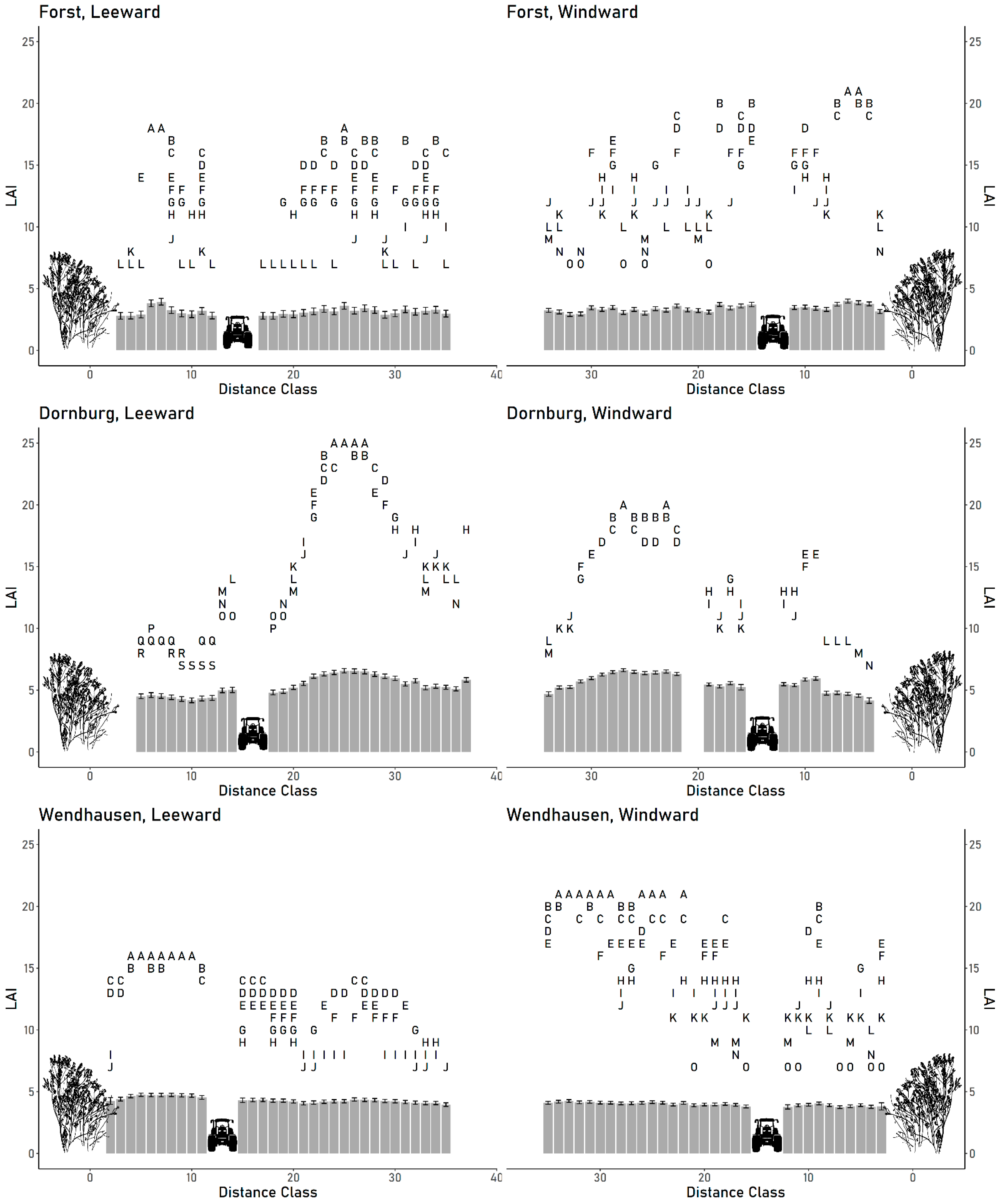
Three German alley cropping agroforestry systems (AFS) located at Forst (51°47′26.6″ N 14°38′05.3″ E), Dornburg (51°00′46.3″ N 11°38′47.1″ E) and Wendhausen (52°19′47.7″ N 10°37′49.0″ E) were sampled in June 2019 (see Figure 1a). At all sites summer barley was grown in 2019. The summer of 2019 was very dry, with precipitation being 27% below the long-term average and soil moisture in the surveyed federal states on the lowest level ever recorded since measurements started in 1961 [1]. Since all experimental sites were established around 10 years ago (see Table 1) by different research institutions, their designs differed considerably in size, crop alley arrangement and tree row characteristics (for detailed site descriptions see [7,49,50]). Although none of the experimental sites was featured by true replicates of the combination of tree rows, alley width and arable crops, sampling plots were placed in sections of the sites where conditions were as similar as possible. The 50 × 96 m plots were placed in 96 m wide crop alleys with adjacent poplar short rotation coppice (SRC) tree rows (see Figure 1c) to enable undisturbed observation of far ranging leeward and windward tree effects on crop parameters. The gap distance between tree and crop rows was planned at 0.8 m (Forst), 1.5 m (Dornburg) and 1.5 m (Wendhausen), however in 2019 the real distances measured with a differential global positioning system (DGPS) were different. At Dornburg the first 2 m adjacent to the western tree row and a 50 cm swath in the eastern part of the plot were accidentally not drilled. Thus, in the current study all distances to trees are given as the real distance of the middle line of the outermost tree row to a place in the crop alley measured with an accuracy of 1.5 cm.

Figure 1.
Experimental Sites. (a) Location of sampled AFS sites within Germany. (b) Photo of AFS site Forst. Footprint of Plot and Subplots are indicated by white lines. (c) Map of AFS site Forst.

Table 1.
Characteristics of eastern and western tree rows at the surveyed AFS sites.
All sites were characterized by western prevailing wind directions. At Forst and Dornburg, the plots were placed at least 50 m away from the endpoints of the tree rows for minimized edge effects, while at Wendhausen this could not be accomplished as this would have resulted in different tree row composition. However, due to different tree harvest years and local growing conditions, the tree height at the surveyed plots ranged from 3 m (Forst, western tree row) to nearly 8 m (Dornburg, western tree row) (see Table 1). While at all sites the hybrid poplar clone “Max” (Populus maximowiczii × Populus nigra) was grown, at Wendhausen tree rows consisted of three blocks of different varieties of poplar clones, namely “Max”, “Hybrid 275” and “Koreana”. The eastern tree row at Wendhausen was featured by two rows of the three aforementioned poplar varieties on each side, while the two rows in the middle were replaced by one row of high growing aspen (Populus tremula).
Within the 50 × 96 m plot, 60 subplots for field sampling, measuring 1 × 1 m, were distributed in a weighted random pattern. The plot was divided into blocks between the tramlines. As highest variability of crop parameter values was expected close to tree rows, the blocks adjacent to the former received 15 randomly distributed subplots, while the three blocks in the center of the plot received 10 subplots each (see Figure 1c).
2.2. UAV-Borne Data Acquisition
Data acquisition using two different UAV-borne sensors, namely a red, green and blue (RGB) and a multispectral sensor, was carried out during milk ripeness (BBCH 75) of barley at all sites (Forst: 15 June; Dornburg: 18 June; Wendhausen: 24 June). This stage was the latest date possible for remote sensing of still green crops, thus remaining time until maturity and harvest (Forst: 24 July; Dornburg: 22 July; Wendhausen: 8 August) was minimal. UAV flights were conducted around solar noon during sunny weather without clouds. Flight times were slightly adjusted to avoid shading on the plots in Dornburg and Wendhausen where tree rows are not aligned in north-south direction.
Red, green and blue (RGB) imagery was acquired utilizing a consumer-grade DJI Phantom 4 photo drone equipped with a DJI FC300S 12-megapixel camera (DJI, Shenzhen, China). Capturing RGB imagery with a low-flying high-resolution platform-sensor-combination instead of using the first three bands of the high-flying multispectral sensor was expected to be necessary to detect the subtle cm-level changes in canopy height across the crop alley. Flight missions were planned with the software Pix4D Capture (version 4.5, Pix4D S.A., Prilly, Switzerland). With the aim of 3D point cloud generation, two flights were carried out per plot at 25 m above ground level (AGL) in a cross-grid pattern whereby every flight covered half of the 50 × 96 m plot plus the adjacent tree strips. Overlap and sidelap of images were set at 80% with a camera angle of 70°. The resulting ground sampling distance (GSD) was approximately 1 cm. For georeferencing and orthorectification, during UAV flights nine wooden 1 m²-sized black and white checkerboard pattern ground control points (GCPs) were placed on modified camera tripods to raise them above the crop canopy. These were evenly distributed in the tramlines within the plot. Their respective X, Y and Z position was determined with a Leica Viva GS14 real-time kinematic (RTK) global navigation satellite system (GNSS) (Leica Geosystems AG, Heerbrugg, Switzerland) at a precision of 1.5 cm.
As the goal of RGB data acquisition was the assessment of crop height from 3D-models, additionally to the flights in June depicting the crop and tree canopy–resulting in the digital surface model (DSM)–another flight was carried out at each site right after drilling of the barley in early 2019 (Dornburg: 28 February; Forst: 3 March; Wendhausen: 12 April). The surface of bare soil after drilling was used for the digital terrain model (DTM), thus enabling canopy surface height (CSH) calculation (DSM–DTM).
Multispectral data was captured using a MicaSense RedEdge-M camera combined with a MicaSense downwelling light sensor (DLS) (Micasense, Seattle, WA, USA). RedEdge-M provides five spectral bands, namely blue, green, red, red edge, near-infrared centered at 475, 560, 668, 717 and 840 nm with full width at half maximum (FWHM) of 20, 20, 10, 40 and 10 nm respectively. A BirdsEyeView Aerobotics FireFLY6 PRO vertical take-off and landing (VTOL) fixed wing UAV (BirdsEyeView Aerobotics, Andover, NH, USA) served as long endurance carrier platform, hence the complete experimental sites could be captured with multispectral imagery in a single flight. Flight planning was conducted using the software FireFLY6 Planner (v. 2.4.0, BirdsEyeView Aerobotics) in a simple grid pattern. Flights were carried out at a height of 100 m AGL with an overlap and sidelap of 75% resulting in a GSD of approximately 6 cm, although real flight speeds, flight tracks and overlaps varied slightly due to wind components. The GCPs used for RGB image acquisition remained in the field for multispectral imaging, while another 18 GCPs made from truck tarpaulin (only X- and Y-coordinates were used) were evenly distributed throughout the rest of the experimental sites. Radiometric reference was captured immediately before and after each flight by means of a MicaSense Calibrated Reflectance Panel.
2.3. Manual Field Sampling
After UAV flights were conducted, the 60 subplots were marked using an RTK GNSS for leaf are index (LAI) determination and destructive biomass sampling. Subplots were arranged parallel to the crop rows.
LAI was measured with a LI-COR LAI-2000 plant canopy analyzer (LI-COR Inc., Lincoln, NE, USA) along a diagonal line inside every subplot. Therefore, one measurement was made above the canopy for reference, followed by four measurements close to the ground where two measurements were taken in the row and two between the rows at intersections with the diagonal of the subplot. The procedure of measurements above and below canopy was repeated once, thus two above- and eight below-measurements were taken in total, resulting in one average LAI value per subplot. If direct sunlight was present, LAI measurements were carried out under the shade of a two meter wide sunshade to avoid error from sunlit leaves [51].
Biomass sampling was carried out through cutting of 33.3 cm of barley rows at ground level at three places within every subplot, depicting the within-subplot-variability as good as possible. The small sample size was chosen so that a large portion of the subplot remained undisturbed for grain yield determination at harvest time. Total fresh matter (FM) of the destructively sampled barley was determined in the field, while an aliquot of FM biomass was dried in the lab for 48 h at 105 °C in a drying oven. Total barley dry matter yield (DM) was calculated subsequently.
2.4. RGB and Multispectral Data Processing
UAV-borne RGB images were processed to 3D models using the photogrammetry software Agisoft Metashape Professional Edition (v. 1.5.5.9097, Agisoft LLC, St. Petersburg, Russia). In a multistep process called structure from motion (SFM), single RGB images were aligned and a point cloud was generated from which a 3D model and a DTM raster could be produced (for detailed process description see [52]). Barley CSH was calculated in the programming language R (v. 4.0.2, [53]) for every subplot by subtracting the DSM point cloud from the DTM raster. In total, twelve CSH variables were calculated for every subplot, namely minimum, maximum, mean, median, standard deviation and mode values as well as 25th, 75th, 90th, 95th and 98th percentiles and the number of points within each subplot. Hereby, the number of points per subplot may have acted as a proxy for barley stand density.
Tree height was derived similarly, yet unlike for barley CSH determination, no reference DTM raster values (RGB data captured in early 2019) were available at the location of every tree point from the DSM point cloud (RGB data captured in June) as no bare soil could be captured under the trees as a reference during drone flights for DTM generation. Thus, median DTM height of a 1 m² area was calculated 3 m away from the tree row inside the crop alley as reference. This was done for every meter along the 50 m long border of the plot with the tree row. Tree height was subsequently calculated from the DTM reference and maximum point cloud values at 1 m long strips of tree row, enabling calculation of one median tree height value for every sampled tree row based on 50 single values.
Multispectral images were processed to orthomosaics as described above for RGB images using Agisoft Metashape. In this process, radiometric calibration was executed automatically using the images of the captured reflectance panels. The mean reflectance per subplot was calculated for all multispectral bands subsequently. Mean reflectance values of all sites were normalized using Equation (1), where xi is a spectral vector for i = 1, …, n [54], in order to take different lighting conditions during data acquisition into account. The mean of normalized reflectance values per 1 m² subplot was calculated as:
For improved exploitation of multispectral reflectance information, vegetation indices, fitting to specific wavelengths covered by the five bands of MicaSense RedEdge-M, were calculated from normalized multispectral reflectance. Six vegetation indices (VIs), namely normalized difference vegetation index (NDVI) [55], soil-adjusted vegetation index (SAVI) [56], renormalized difference vegetation index (RDVI) [57], red green blue vegetation index (RGBVI) [37], normalized difference red edge index (NDRE) [58] and enhanced vegetation index (EVI) [59] (see Equations (A1)–(A6) in the Appendix A), were used, of which NDVI, RGBVI and SAVI have shown to improve prediction of barley biomass yield in conjunction with plant height dependent on plant development stages [37,38]. Their respective mean value was calculated for every subplot.
In an effort to better depict small-scale spatial variability (‘non-homogeneity’ [60]) of DM and LAI values which might be linked to changes in reflectance values, texture was considered a viable factor. “Texture is characterized not only by the gray value at a given pixel, but also by the gray value ‘pattern’ in a neighbourhood surrounding the pixel” [61]. Texture measures can be calculated in the form of a grey level co-occurrence matrix (GLCM), where relative frequencies of grey levels of two neighbouring pixels, a function of their angular relationship as well as their distance, are stored in a matrix representing their spatial dependencies [62]. Haralick [62] proposed a set of 23 textural features, eight of which were used in the present study utilising function ‘glcm’ from R package ‘glcm’ (v. 1.6.5., [63]): ‘mean’, ‘variance, ‘homogeneity, ‘contrast, ‘dissimilarity’, ‘entropy, ‘second moment’ and ‘correlation’ (for equations see [62]). Crop rows in combination with high spatial resolution (GSD 6 cm) gave reason to expect texture features to be rotation dependent, thus rotation invariant features were calculated with shifts in all directions (0, 45, 90 and 135°) and a window size of 7 × 7 pixels, covering multiple crop rows. We believe this helped to ensure that texture variables did not depict expected differences in grey levels between pixels in a crop row and between crop rows but rather gaps in the canopy or stand density. From every texture feature calculated (8 features) for every multispectral band (five bands), mean, minimum, maximum and median values per subplot were calculated, adding up to a total of 160 texture variables.
2.5. Random Forest Regression Model Building
The two yield-related crop parameters DM and LAI were modelled from the normalized reflectance, VIs, texture and plant height variables (see above). The number of samples in the modelling process was 176 as two samples had to be removed due to trees obscuring the subplots at Dornburg and Wendhausen. As these parameters are characterized by a high collinearity, random forest regression (RFR) was used, which is a proven non-parametric regression algorithm for estimation of plant traits from spectral data that can deal with multicollinear data [64,65]. It can be utilized smoothly with the packages ‘classification and regression training’ (caret v. 6.0-86, [66]) in conjunction with package ‘variable selection using random forests’ (VSURF v. 1.1.0, [67]) to reduce computational resources and the risk of overfitting. In this study, for DM and LAI the total of 183 predictive variables was reduced to 19 and 11 variables, respectively. After variable selection a stratified random split of the reduced dataset into a calibration (80% of data) and a validation (20% of data) set was conducted, ensuring that samples from all sites as well as all blocks of every site were included (n = 176) (see Figure 2). Therefore, five blocks per site were defined from west to east, confined by the tramlines running through the plot as spatial variability of DM and LAI values was expected to vary mainly in the direction perpendicular to the tree rows (see Section 2.1). Model calibration was repeated in 100 iterations, as it turned out that modelling results varied depending on the samples randomly selected for calibration and validation. Modelling performance, judged by the metrics R²p and nRMSEp, with:
where ymax and ymin are the maximum and minimum observed values, was calculated with the 100 corresponding validation datasets in form of the median value of 100 iterations. The importance of predictive variables in the training process was determined using the function ‘varImp’ from package ‘caret’. The model performance was optimized by tuning of its ‘hyper-parameter’ to an optimal value. The number of variables within a tree considered for each split in the training subset defined through the ‘hyper-parameter’ ‘mtry’ is thought to be “the primary tuning parameter, and has its greatest impact on the complexity of the final model” [68]. During model calibration (100 iterations), the ‘hyper-parameter’ defining the number of drawn candidate variables per split (‘mtry’) was optimized through repeated cross-validation (ten folds, five repeats) to a median value (most frequently occurring) of 5 and 4 randomly selected variables considered as split candidates per tree for DM and LAI respectively. To achieve a good balance between computational time and error, the number of trees was set at a value of 500 trees while node size, defining tree complexity, was kept constant at a value of 5 [68]. Final models for DM and LAI map prediction based on 100% of the data were calibrated subsequently with the optimal ‘hyper-parameters’ through repeated cross-validation (10 folds, five repeats).

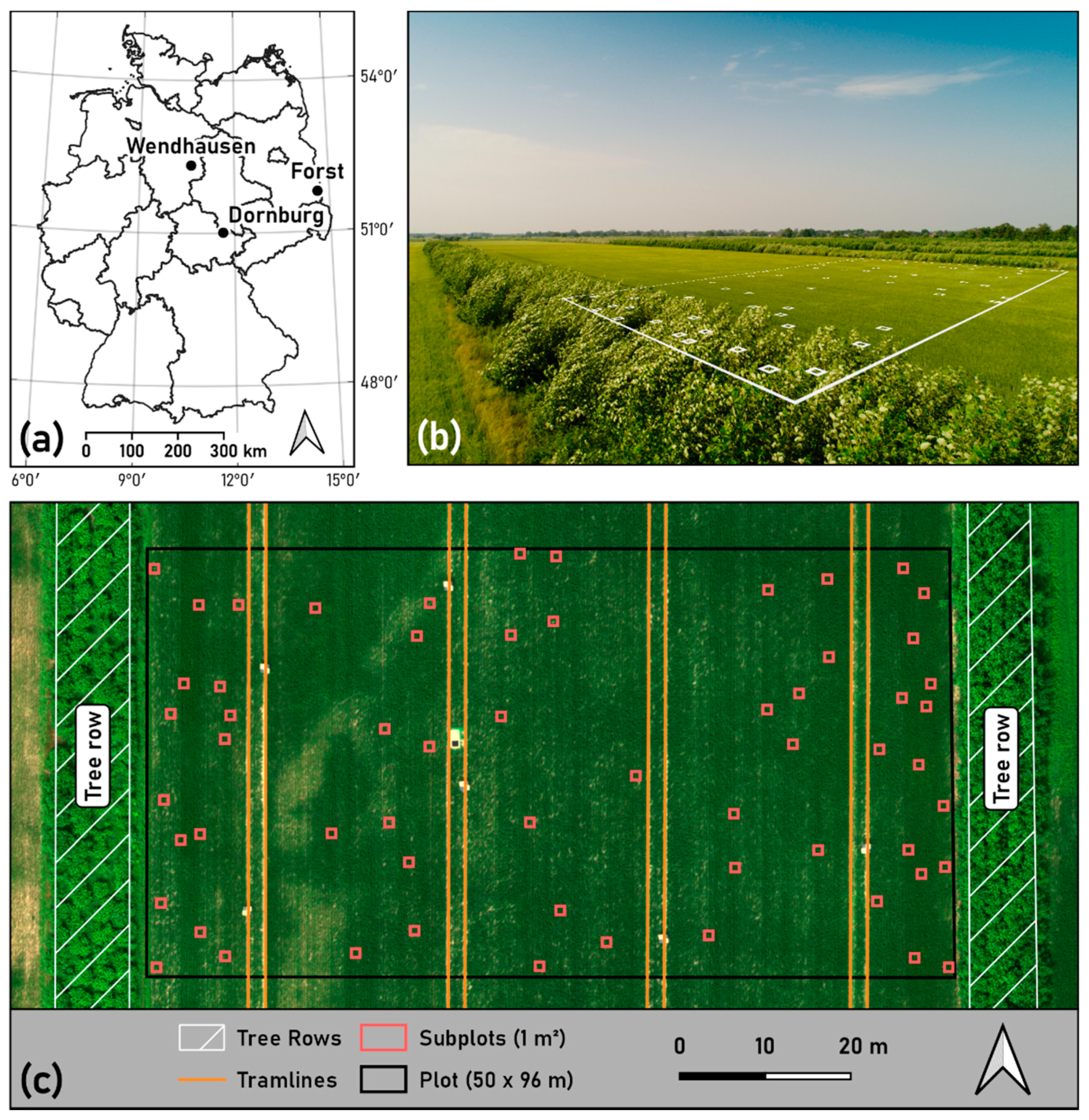
Figure 2.
Workflow of model building, point data generation and spatial analysis.
2.6. Map and Point Data Generation
Maps for DM and LAI based on the final models were predicted for the entire sampling plot at every site. Therefore, raster files of all predictive variables selected by VSURF were calculated at a spatial resolution of 1 m, as the reference sample size during destructive field sampling was 1 m². While a raster with mean values per m² was calculated for each normalized reflectance band and each VI, for CSH and texture variables a raster containing the respective value per m² (minimum CSH value for ‘csh_min’, median correlation value for ‘B2_tex_median_cor’, number of points for ‘csh_freq’ etc.) was calculated based on high resolution point cloud and multispectral data. From predicted maps with 1 m spatial resolution all 1 m² pixels close to the tree rows containing trees were clipped. The same applied to regions of the plot in Dornburg, where barley plants were damaged from walking through the plot as the schedule of fieldwork had to be re-arranged due to problems with a UAV. Therefore, all 1 m pixels containing areas with damaged plants were deleted generally to prevent misinterpretation of erroneous spatial patterns.
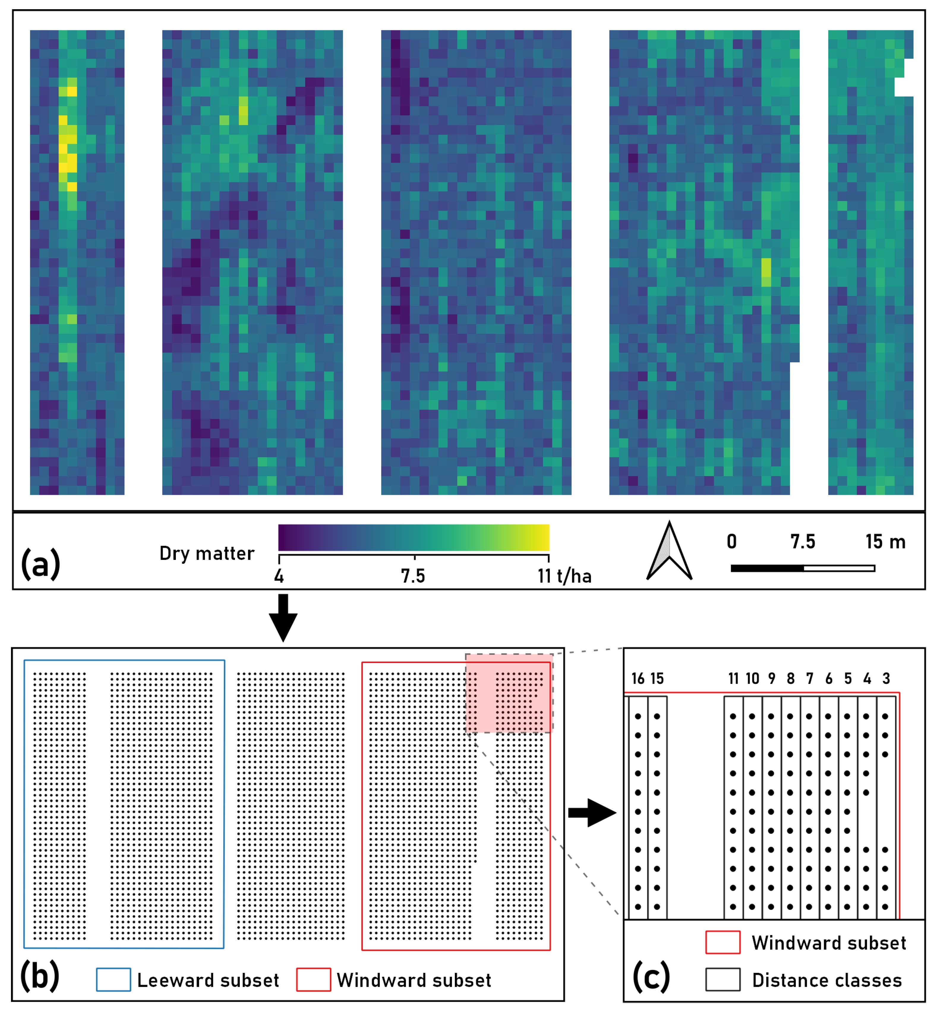
For spatial analysis with mixed models, the predicted maps were converted to point data. This was accomplished through assignment of the respective DM/LAI value to the central location of each pixel (see Figure 3a,b). Derived point values for every site were split into two subsets, namely a leeward (western) and a windward (eastern) subset. All point values ranging from the nearest tree row through to the second tramline within the plot were assigned to the respective subset (see Figure 3b). A distance of about 35 m from the tree row was considered far enough to depict the effects of trees on barley DM and LAI. For every point, the distance to the tree row was calculated based on the real distance to a line running through the outermost trees of the tree row closest to the crop alley. In order to enable mean comparisons of DM and LAI values depending on distance to trees, 1 m wide distance classes were created. All points between 2.5 and 3.5 m away from the tree row were assigned to the distance class 3 and so forth (see Figure 3c). Consequently, as the plot border along the tree row was 50 m in length, every distance class contained a maximum of 50 observations if no pixel had to be clipped.

Figure 3.
Generation of point data from predicted raster data. (a) Predicted DM at AFS site Forst. Spatial resolution is 1 m. (b) Generated point values and subsets from the raster. (c) Distribution of 1 m wide distance classes (real distance to tree row).
2.7. Spatial Analysis Using Linear Mixed Models
Spatial analysis of leeward and windward subsets for DM and LAI of all sites were tested independently with linear mixed models (LMM) for correlation with distance to tree row and mean comparisons between distance classes. LMMs were utilized due to their ability to account for the spatial correlation among unequally spaced samples within the same plot [48]. Statistical analyses were carried out in SAS University Edition (SAS v. 9.4, SAS Studio Release 3.8 Basic Edition, SAS Institute Inc., Cary, NC, USA) using the procedure ‘glimmix’ with an anisotropic power model. Distance class was defined as the fixed effect with the random effect covering spatial autocorrelation. The variance-covariance structure of the random effect was depicted with an anisotropic power model accounting for different spatial correlation in X- and Y-direction [69]. Degrees of freedom were calculated using the Kenward-Roger method. Studentized residual plots were examined for homogeneity of variance and normal distribution of the residuals [70]. Adjusted means for effect ‘distance class’ were computed with statement ‘lsmeans’ and significance of differences between all distance classes of each subset were tested by t-test (p < 0.05) using option ‘pdiff’. Confidence limits (95%) were given indicating sample sizes per distance class. Significant differences between distance class means were visualized using a letter display [71].
3. Results
3.1. Field Data: Yield-Related Crop Parameters
Values of the parameters DM and LAI measured at the subplots of every site revealed large differences between the sites (see Table 2). Values of DM and LAI followed a similar pattern where Dornburg showed the highest values (mean DM 10.3 t/ha; mean LAI 5.3) followed by Wendhausen (mean DM 7.7 t/ha; mean LAI 4.2) and Forst (mean DM 6.8 t/ha; mean LAI 3.3). Barley DM yields at Wendhausen and Forst most likely were reduced due to draught conditions being more severe than at Dornburg, where DM yield was comparably high [72]. Values of DM and LAI were characterized by a big range at all sites. Across sites they varied between 2.2 and 17.4 t/ha DM and between 2.3 and 7.4 for LAI. Low values were observed not only at subplots near tree rows, where they were expected, but throughout the entire crop alley.
Table 2.
Descriptive statistics for DM and LAI values measured at subplots (SD = standard deviation, CV = coefficient of variation).
3.2. Random Forest Regression Model Performance
Modelling of DM and LAI from spectral data and 3D-point clouds using a random forest regression algorithm resulted in acceptable prediction precision and accuracy for DM (median R²p 0.62, median RMSEp 1.63 t/ha, median nRMSEp 14.9%) and good precision and accuracy for LAI (median R²p 0.92, median RMSEp 0.3, median nRMSEp 7.1%). Single models yielded much higher prediction precisions (see Table 3) but were not considered relevant, as stratified random sample selection for calibration and validation in 100 iterations indicated overoptimistic model assessment from single selections.
Table 3.
Model performance for DM and LAI prediction. Minimum, maximum and median values of 100 model runs with different randomly selected calibration (80%) and validation (20%) samples.
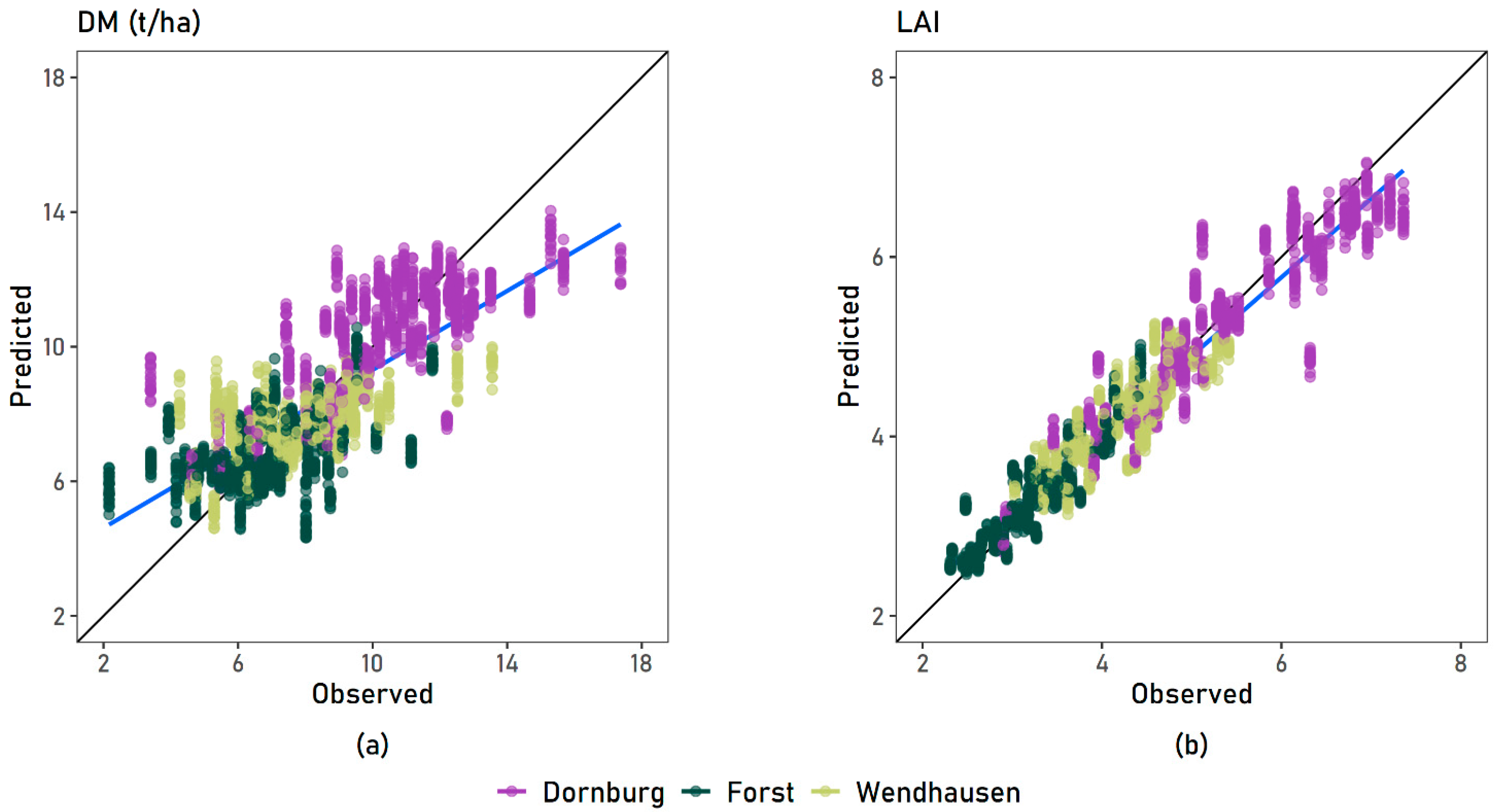
The plot of fit for DM (see Figure 4a) revealed an overestimation of low DM as well as an underestimation of high DM values, while variation of values from 100 iterations was similarly pronounced throughout the whole range. Clusters could be observed for values originating for the same site reflecting their different growing conditions. LAI was predicted well along the complete range with high values being slightly underestimated (see Figure 4b).

Figure 4.
Observed versus predicted values for (a) DM and (b) LAI at each sampling site. Values from all sites were included in the model, represented by different colors. Blue line is the regression line, black line is 1:1 line.
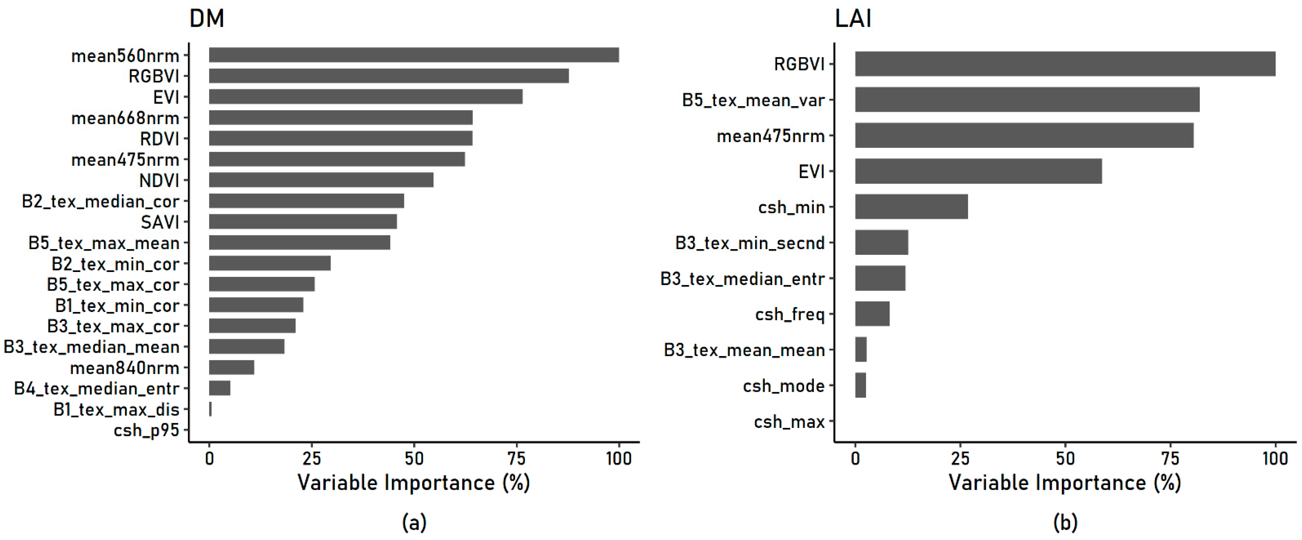
The most important variables for prediction of DM were normalized multispectral reflectance (green, red and blue bands), VIs (RGBVI, EVI, RDVI and SAVI), and texture variables, especially correlation (‘_cor’) calculated from different bands (‘B2’, ’B5’ etc.) (see Figure 5a). CSH information obtained from RGB imagery played a negligible role in DM prediction. Interestingly, normalized red edge and near-infrared reflectance were not among the important variables for prediction, however, they were still indirectly included through indices.

Figure 5.
Variable importance of all variables selected by variable selection using random forests (VSURF) for (a) DM and (b) LAI prediction. Prediction is based on (a) normalized reflectance (e.g. “mean560nrm”), vegetation indices (e.g. “EVI”), texture variables (e.g. “B2_tex_median_cor”) and canopy surface height metrics (e.g. “csh_p95”).
VIs calculated from normalized multispectral reflectance (RGBVI, EVI), texture variables and normalized multispectral reflectance (blue band) ranged among the most important variables for LAI prediction as well (see Figure 5b). As opposed to DM, several CSH variables were important for the prediction of LAI. Among them were minimum CSH (‘csh_min’) as well as the number of points from the point cloud per subplot (‘csh_freq’). Both variables are related to the density of the barley population as gaps in the canopy influence minimum values as well as the total number of points through the surface being more inhomogeneous or rough at a given spatial resolution. CSH metrics are known to offer another improving (third) dimension for LAI and DM prediction [73], otherwise restricted by saturation at high values [74]. Prediction of DM and LAI from a dataset without CSH variables, hence, reduced to variables calculated from multispectral reflectance only, revealed a similar prediction accuracy, with CSH only slightly reducing the error. In the present study, the analyzed crop traits could have been predicted from a single multispectral sensor platform combination, reducing cost and labor significantly.
For both DM and LAI predictions, calculation of GLCM texture variables improved the prediction accuracies. Texture most likely provided a way to take homogeneity of the population into account, as with 6 cm GSD, gaps in the canopy could be represented by the spatial variability of pixel values.
3.3. Spatial Variability in Crop Traits
Maps produced with the best models for DM and LAI offered a detailed view at the spatial variability across the crop alley (see Figure 6). Although resampled to a resolution of 1 m, clear spatial patterns could be observed at all sites. Low values of DM and LAI tended to be aggregated close to the tree rows, however no clear tree induced pattern prevailing across all sites could be found.

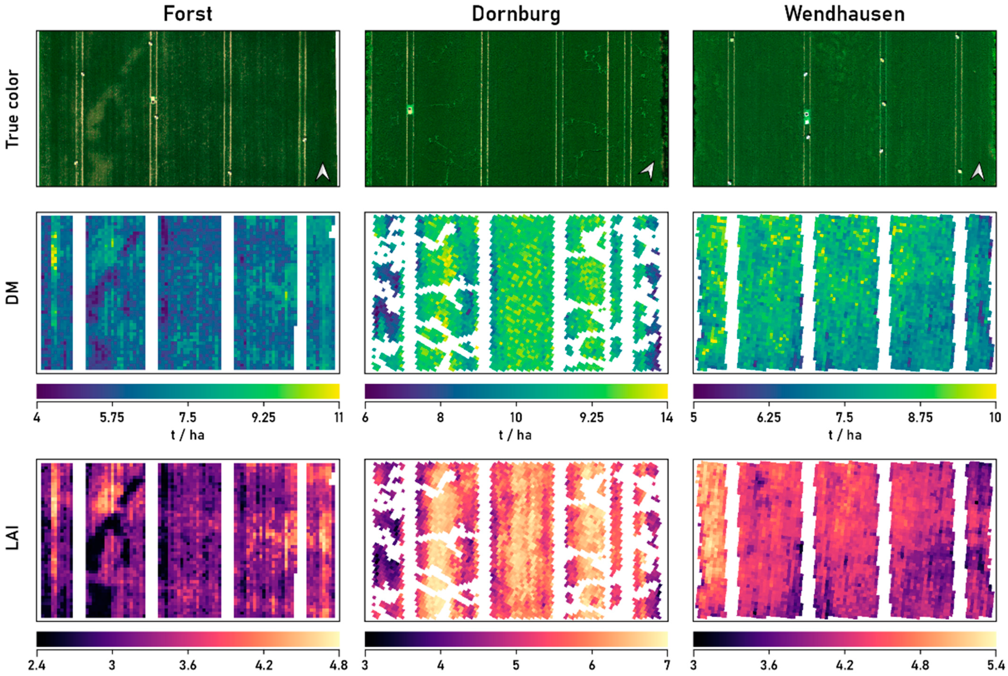
Figure 6.
Predicted maps for barley DM and LAI at milk ripeness (BBCH 75) at three study sites. Color scales differ between sites for improved visibility of spatial variability. Maps for AFS sites Dornburg and Wendhausen were rotated (see north arrow in true color map). Gaps in maps for Dornburg stem from damage done to barley plants during fieldwork (mixed 1 m pixels were deleted generally to prevent misinterpretation of erroneous spatial patterns).
At Forst, patches of low DM and LAI values in the western part of the plot most likely are a result of different soil conditions. If areas surrounding the plot were considered as well, the patches in the plot could be identified as part of a former meander of the river Neisse, nowadays running close by. Additionally, linear structures in west-northwestern to west-southwestern direction pointed at drainage pipes running through the plot. High DM and LAI values in a 3 m wide strip at the western part of the plot seemed to originate from interventions of the farmer such as overlapping during drilling.
Due to damage during fieldwork at Dornburg parts of the plot had to be clipped. However, a clear spatial pattern could be observed. Pronounced strongest for LAI, highest values were found in the middle of the crop alley and furthest away from tramlines. Low values were found close to the tree rows. This spatial pattern was visible best at Dornburg, possibly due to tree height and density being highest there.
No clear relation to tree height could be found at Wendhausen, where trees were highest in the eastern tree row but no visible reduction in DM or LAI could be observed. Instead, a trend from northwest to southeast could be detected, potentially resulting from edge effects as the tree rows ended close to the southern end of the plot and the prevailing wind direction was west.
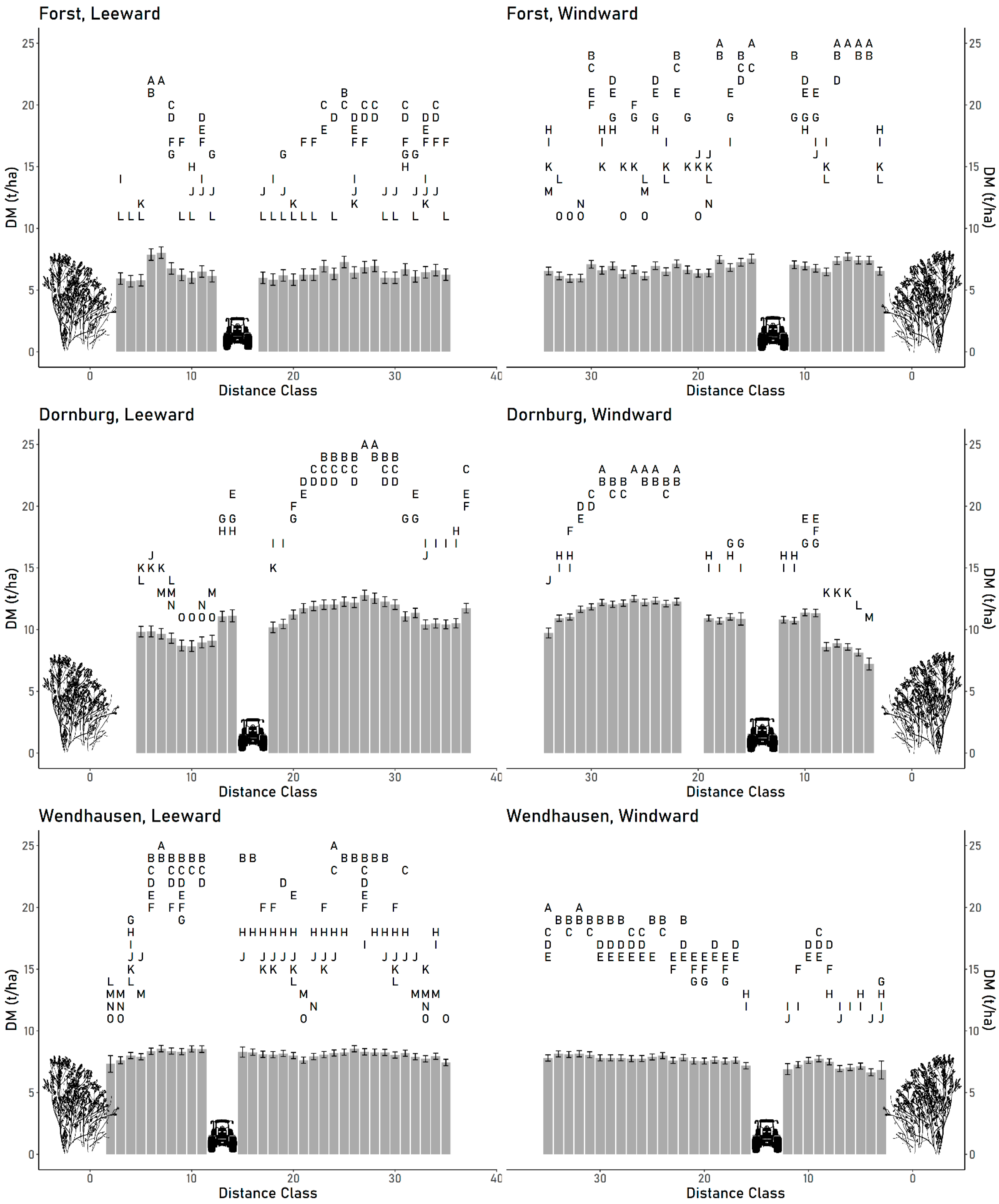
Analysis of spatial variability using mixed models showed a significant effect (p < 0.05) of distance class on DM and LAI at all sites and subsets (leeward, windward). Comparisons of least squares means between distance classes supported findings from the analysis of the maps (see Figure 6). Only at Dornburg, DM was significantly lower close to the western and eastern tree rows compared to the rest of the crop alley (see Figure 7). Yield depression might have been more strongly pronounced close to the western tree row due to increased shadow resulting from orientation of the tree row. A clear effect of proximity to tramlines could be found at Dornburg, where DM and LAI were significantly higher at distance classes far away from the tramlines. At Forst, distance classes close to the tree row had significantly higher DM yields as well as LAI values (see Figure A1), possibly resulting from management effects masking tree effects. The declining trend from west to east observed in the maps for Wendhausen was confirmed through significantly lower DM and LAI values in eastern direction only overlaid in the leeward subset by tree effects in distance classes adjacent to the tree row.

Figure 7.
Comparisons of barley total dry matter (DM) least squares means between distance classes. Distance classes for leeward and windward plots are based on real distance to western and eastern tree rows. Distances having no letter in common are significantly different (α = 0.05). Error bars show 95% confidence limits.
4. Discussion
Detailed spatial analysis of tree effects on yield are of utmost importance for a solid understanding of tree-crop interactions occurring in agroforestry systems (AFS). However, only one study has made use of high-resolution unmanned aerial vehicle (UAV)-borne imagery to study the range of tree effects on yield in an African AFS characterized by solitary trees [47]. No study has analyzed spatial variability of yield-related parameters in intensively managed alley cropping systems (ACS) at high spatial resolution utilizing UAV-borne data yet. The present study demonstrates a novel way to analyze yield-related spatial effects in ACS, employing UAV-borne imagery for modelling and map generation.
4.1. Model Performance
Random forest regression (RFR) models for barley whole crop dry biomass (DM) and leaf area index (LAI) built from UAV-borne images achieved good prediction accuracies. LAI could be predicted with high accuracy which is in line with previous findings [75,76,77] and was expected due to the strong correlation of reflectance in the visible spectrum and leaf pigments per area [78]. Different crop density near tree rows, indirectly reflected by LAI, thus was accurately depicted by the presented models. The results for DM prediction are comparable to other studies on crop aboveground biomass (AGB), considering the advanced crop maturity stage and use of a broadband multispectral sensor. Utilizing a hyperspectral sensor, Yue et al. [41] could predict wheat AGB with slightly better results (R²val 0.74, RMSEval 1.2 t/ha). Näsi et al. [79] predicted barley DM at an early growth stage from hyperspectral and RGB images with high Pearson’s correlation coefficient (r = 0.95) but much higher relative root-mean-square error (RMSE 33.3%). In another study on barley, the higher correlation of DM (R² 0.83) with visible spectrum vegetation indices (VIs) and canopy surface height (CSH) may be explained by the multitemporal nature of the data acquisition throughout the growing season [37]. The same study reported that predictions deteriorated at late development stages of the barley crop, which likewise applies in the present study due to the proximity to harvest date. The use of a hyperspectral sensor likely also improved prediction accuracy as its narrow spectral bands allowed a better depiction of important spectral regions for VI calculation [80].
Addition of gray level co-occurrence matrix (GLCM) texture variables improved the prediction of DM and LAI, as was reported by other studies [40,81]. It is likely that texture variables calculated from high-resolution imagery offered additional information in areas of the plot with gaps in the canopy as prevailing in proximity to tree rows. The importance of texture variables for prediction (Figure 5) seemed to confirm the assumption that at a ground sampling distance (GSD) of 6 cm differing reflectance from barley crop and soil could be covered by a window size of 7 × 7 pixels. Texture, thus, might be a promising feature for future analysis of spatial heterogeneity in AFS.
Contrary to previous results [37,39,41,82], inclusion of CSH variables did not improve model performance significantly. Although CSH variables were amongst the most important variables for prediction of LAI (Figure 5b), model generation without the use of height information did not lead to significantly lower accuracies. An explanation could be the use of growth regulator in the crop in at least one occasion at Dornburg. Through equalized plant height, the correlation between height and DM and LAI could have been obliterated. As CSH variables were the only features derived from RGB data, data acquisition could have been reduced to one flight with a multispectral sensor. For practical field work and data processing this is very relevant, since 3D-Model generation requires many images captured from different angles and extensive computer resources. Capturing RGB images of the 50 × 120 m plot (including tree rows) for a structure from motion (SFM) approach at 1 cm GSD in the present study took almost as long as capturing multispectral images of an entire AFS site (40 ha) with a GSD of 6 cm.
Out of the variables calculated from multispectral data, besides normalized reflectance and texture variables, VIs proved their high value for crop DM and LAI estimation as was shown in other studies [37,38,45]. Among them, the red, green, blue vegetation index (RGBVI) developed by Bendig et al. [37] for barley DM estimation proved to be one of the most important variables for prediction in this study for DM as well as for LAI.
Modelling of yield-related variables with the use of machine learning algorithm RFR, as was demonstrated in previous studies [46,79,83], delivered solid results. The implementation of RFR in the R environment with possible integration of a variable selection step makes it an efficient tool. New machine learning algorithms such as neural networks [32], however, might further improve prediction accuracies. Another important step in model advancement might lie in spatial variable selection and validation strategies, highlighted by recent studies [84,85]. A significant improvement of modelling performance might be achieved through inclusion of data on soil type and a higher number of samples with a larger sampling area, thus representing the local conditions better. In the current study, only 1 m of crop row was harvested as the same subplots were to be analyzed for grain yield during harvest. It is expected that increasing the subplot size to 1 m² would increase measurement precision considerably, while still allowing highly detailed mapping.
4.2. Spatial Analysis
Statistical analysis of the effect of distance to tree row using linear mixed models (LMMs) confirmed a significant effect on DM and LAI values. Contrary to the authors expectations, point data of DM and LAI were highly correlated (R = 0.94, n = 7273). Regarding significant differences between least-squares means of distance classes, the frequently observed typical pattern of low yield near tree rows, increased yield in a transition zone and normal yield in the middle of the crop alley was not observed at the surveyed AFS sites. Though this spatial pattern was found in various studies [86,87,88], all three surveyed sites showed different DM and LAI distributions, seemingly strongly influenced by varying soil conditions and management effects, such as distance to tramlines (see Figure 6). It has to be pointed out, however, that due to shade and trees concealing crops very close to tree rows from above, parts of that area had to be clipped and left out from the analysis.
Numerous studies have analyzed tree effects in relation to tree height [12,14,89,90], which is an easy measure to collect during field work. However, the present study indicated the weakness of this metric, as for example at Wendhausen DM and LAI values were lower near the eastern tree row compared to the western tree row although trees were about three meters higher in the east (see Figure 6 and Table 1). The spatial trend in DM and LAI values at Wendhausen from west to east might be explained by edge effects at the end of the tree row or by changing soil conditions. Still, tree height alone could not explain the pattern, suggesting that a metric for tree density might supplement a better understanding of tree effects. UAV-borne volume based estimation of tree biomass, as described by Lingner et al. [91], could pave the way to improve the understanding of the effect of tree row density on crop yield.
At the surveyed leeward and windward sections of crop alleys, barley DM and LAI was significantly lower compared to other distance classes only within the first few meters adjacent to the tree rows if at all. These findings are in line with previous studies analyzing tree effects on yield from windbreaks [92,93] and short rotation coppice (SRC) tree rows in ACS [15,16]. The current study, however, did not employ geostatistical methods to analyze the range of tree effects directly, as proposed by Roupsard et al. [47]. Although tested, non-stationarity prevented variogram analysis of point data generated from predicted maps. Exploring the maps of DM and LAI values at Forst strongly indicated management and soil conditions dominating yield-related parameters across large parts of the crop alley. Apart from clearly demonstrating the dangers of transect-based methods at this site, determining a ‘range’ of tree effects under these conditions might be misleading. Admittedly, the analysis with LMMs could not answer the question of tree effect range, yet it offers valuable insights into significant spatial differences of yield-related parameters in ACS.
The method proposed in this study is a significant improvement in information density compared to previous transect based methods commonly employed in AFS studies [15,16]. There, samples are taken at four distances from the tree row, leaving wide swathes of the field unsampled. Additionally, two ‘replicates’ are taken within the same tree row, thus being sensitive to spatial trends in soil conditions and effects of tillage and fertilizer application, which is done parallel to the tree rows. In contrast, UAV-borne measurements offer cm-level resolution as well as possible coverage of entire agroforestry sites within one flight. However, as expected, one of the most important agricultural metrics, namely grain yield, could not be predicted from remotely sensed imagery in the present study based on a single measurement date. Manual measurements during harvest, thus, cannot be replaced by drone flights yet. Additionally, one should consider that model calibration still needs a great amount of destructively sampled reference samples before models could be used to map barley DM and LAI. Taken as a whole, although some restrictions on practical applicability remain, UAV-borne mapping of yield-related crop parameters provides a promising, new method for spatial analysis of alley cropping AFS.
5. Conclusions
The present study could show that total crop dry biomass yield (DM) and leaf area index (LAI) of barley can be modelled with good accuracy from UAV-borne imagery at three different AFS sites. Produced maps enabled detailed spatial analysis of tree effects on yield. Distance to tree had a significant effect on DM and LAI, however it was likely overlaid by soil and management effects in large parts of the crop alley. Though the limited database of the study prevents generalized statements on spatial effects in AFS, the study demonstrated that the proposed method can be utilized for future investigations of spatial variability of crop DM and LAI in AFS with the goal of a better understanding of tree-crop interactions. As the method is able to cover entire fields at high spatial resolution, it may be used to survey tree effects across more different sites and regions to fill the knowledge gap regarding reasons for spatial variability of crop yield in AFS.
Author Contributions
M.W. (Michael Wachendorf), T.A., R.G. and M.W. (Matthias Wengert) conceptualized the idea of the study; M.W. (Matthias Wengert) processed the data and analyzed the results; J.W. and T.A. assisted data analysis and provided scripts; H.-P.P. assisted in statistical analysis; M.W. (Matthias Wengert) wrote the original manuscript draft; M.W. (Michael Wachendorf), T.A. and R.G. supervised the work, contributed to the interpretation of the results and edited the manuscript. R.G., T.A. and M.W. (Michael Wachendorf) acquired funding for the project. All authors have read and agreed to the published version of the manuscript.
Funding
This work was funded by the German Ministry of Education and Research (BMBF) as a part of the research project SIGNAL (Sustainable intensification of agriculture through agroforestry) within the Framework Program BONARES (Soil as a sustainable resource for the bioeconomy).
Data Availability Statement
The raw data, produced raster files of obtained metrics (e.g. vegetation indices, texture and canopy surface height) and scripts supporting the conclusions of this article will be made available by the authors on request without undue reservation.
Acknowledgments
The authors would like to thank the whole team of GNR for the help during field work and manuscript preparation. We are particularly grateful for the assistance given by Andrea Gerke, Eva Wiegard and Claudia Thieme-Fricke. We would also like to thank our project partners from BTU Cottbus, TLLLR Dornburg and JKI Braunschweig who supported us during data acquisition.
Conflicts of Interest
The authors declare no conflict of interest.
Appendix A
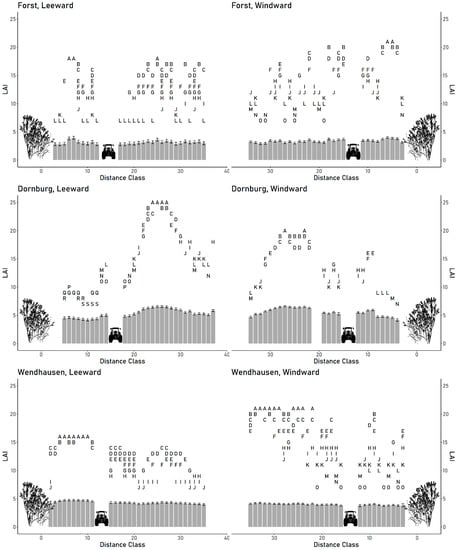
Figure A1.
Comparisons of barley leaf area index (LAI) least squares means between distance classes. Distance classes for leeward and windward plots are based on real distance to western and eastern tree rows. Distances having no letter in common are significantly different (α = 0.05). Error bars show 95% confidence limits.
References
- Deutscher Wetterdienst Deutschlandwetter Im Sommer. 2019. Available online: https://www.dwd.de/DE/presse/pressemitteilungen/DE/2019/20190830_deutschlandwetter_sommer2019_news.html (accessed on 4 May 2021).
- Seibold, S.; Gossner, M.M.; Simons, N.K.; Blüthgen, N.; Müller, J.; Ambarlı, D.; Ammer, C.; Bauhus, J.; Fischer, M.; Habel, J.C.; et al. Arthropod Decline in Grasslands and Forests Is Associated with Landscape-Level Drivers. Nature 2019, 574, 671–674. [Google Scholar] [CrossRef] [PubMed]
- Ray, D.K.; Gerber, J.S.; MacDonald, G.K.; West, P.C. Climate Variation Explains a Third of Global Crop Yield Variability. Nat. Commun. 2015, 6, 5989. [Google Scholar] [CrossRef] [Green Version]
- Kumar, V. Multifunctional Agroforestry Systems in Tropics Region. Nat. Environ. Pollut. Technol. 2016, 15, 365–376. [Google Scholar]
- Smith, J.; Pearce, B.D.; Wolfe, M.S. Reconciling Productivity with Protection of the Environment: Is Temperate Agroforestry the Answer? Renew. Agric. Food Syst. 2013, 28, 80–92. [Google Scholar] [CrossRef]
- Mbow, C.; Smith, P.; Skole, D.; Duguma, L.; Bustamante, M. Achieving Mitigation and Adaptation to Climate Change through Sustainable Agroforestry Practices in Africa. Curr. Opin. Environ. Sustain. 2014, 6, 8–14. [Google Scholar] [CrossRef] [Green Version]
- Böhm, C.; Kanzler, M.; Freese, D. Wind Speed Reductions as Influenced by Woody Hedgerows Grown for Biomass in Short Rotation Alley Cropping Systems in Germany. Agrofor. Syst. 2014, 88, 579–591. [Google Scholar] [CrossRef]
- Palma, J.H.N.; Graves, A.R.; Burgess, P.J.; Keesman, K.J.; van Keulen, H.; Mayus, M.; Reisner, Y.; Herzog, F. Methodological Approach for the Assessment of Environmental Effects of Agroforestry at the Landscape Scale. Ecol. Eng. 2007, 29, 450–462. [Google Scholar] [CrossRef] [Green Version]
- Wang, Y.; Zhang, B.; Lin, L.; Zepp, H. Agroforestry System Reduces Subsurface Lateral Flow and Nitrate Loss in Jiangxi Province, China. Agric. Ecosyst. Environ. 2011, 140, 441–453. [Google Scholar] [CrossRef]
- Bergeron, M.; Lacombe, S.; Bradley, R.L.; Whalen, J.; Cogliastro, A.; Jutras, M.-F.; Arp, P. Reduced Soil Nutrient Leaching Following the Establishment of Tree-Based Intercropping Systems in Eastern Canada. Agrofor. Syst. 2011, 83, 321–330. [Google Scholar] [CrossRef]
- Beuschel, R.; Piepho, H.-P.; Joergensen, R.G.; Wachendorf, C. Similar Spatial Patterns of Soil Quality Indicators in Three Poplar-Based Silvo-Arable Alley Cropping Systems in Germany. Biol. Fertil. Soils 2018. [Google Scholar] [CrossRef]
- Quinkenstein, A.; Wöllecke, J.; Böhm, C.; Grünewald, H.; Freese, D.; Schneider, B.U.; Hüttl, R.F. Ecological Benefits of the Alley Cropping Agroforestry System in Sensitive Regions of Europe. Environ. Sci. Policy 2009, 12, 1112–1121. [Google Scholar] [CrossRef]
- Bailey, N.J.; Motavalli, P.P.; Udawatta, R.P.; Nelson, K.A. Soil CO2 Emissions in Agricultural Watersheds with Agroforestry and Grass Contour Buffer Strips. Agrofor. Syst. 2009, 77, 143–158. [Google Scholar] [CrossRef]
- Tsonkova, P.; Böhm, C.; Quinkenstein, A.; Freese, D. Ecological Benefits Provided by Alley Cropping Systems for Production of Woody Biomass in the Temperate Region: A Review. Agrofor. Syst. 2012, 85, 133–152. [Google Scholar] [CrossRef]
- Kanzler, M.; Böhm, C.; Mirck, J.; Schmitt, D.; Veste, M. Microclimate Effects on Evaporation and Winter Wheat (Triticum aestivum L.) Yield within a Temperate Agroforestry System. Agrofor. Syst. 2019, 93, 1821–1841. [Google Scholar] [CrossRef]
- Swieter, A.; Langhof, M.; Lamerre, J.; Greef, J.M. Long-Term Yields of Oilseed Rape and Winter Wheat in a Short Rotation Alley Cropping Agroforestry System. Agrofor. Syst. 2018. [Google Scholar] [CrossRef] [Green Version]
- Pardon, P.; Reubens, B.; Mertens, J.; Verheyen, K.; De Frenne, P.; De Smet, G.; Van Waes, C.; Reheul, D. Effects of Temperate Agroforestry on Yield and Quality of Different Arable Intercrops. Agric. Syst. 2018, 166, 135–151. [Google Scholar] [CrossRef]
- Graves, A.R.; Burgess, P.J.; Palma, J.; Keesman, K.J.; van der Werf, W.; Dupraz, C.; van Keulen, H.; Herzog, F.; Mayus, M. Implementation and Calibration of the Parameter-Sparse Yield-SAFE Model to Predict Production and Land Equivalent Ratio in Mixed Tree and Crop Systems under Two Contrasting Production Situations in Europe. Ecol. Model. 2010, 221, 1744–1756. [Google Scholar] [CrossRef] [Green Version]
- Seserman, D.; Veste, M.; Freese, D.; Swieter, A.; Langhof, M. Benefits of agroforestry systems for land equivalent ratio—Case studies in Brandenburg and Lower Saxony, Germany. In Proceedings of the 4th European Agroforestry Conference-Agroforestry as Sustainable Land Use, Nijmegen, The Netherlands, 28–30 May 2018; pp. 26–29. [Google Scholar]
- Mead, R.; Willey, R.W. The Concept of a ‘Land Equivalent Ratio’ and Advantages in Yields from Intercropping. Exp. Agric. 1980, 16, 217–228. [Google Scholar] [CrossRef] [Green Version]
- Seserman, D.-M.; Freese, D.; Swieter, A.; Langhof, M.; Veste, M. Trade-Off between Energy Wood and Grain Production in Temperate Alley-Cropping Systems: An Empirical and Simulation-Based Derivation of Land Equivalent Ratio. Agriculture 2019, 9, 147. [Google Scholar] [CrossRef] [Green Version]
- Raatz, L.; Bacchi, N.; Walzl, K.P.; Glemnitz, M.; Müller, M.E.H.; Joshi, J.; Scherber, C. How Much Do We Really Lose?—Yield Losses in the Proximity of Natural Landscape Elements in Agricultural Landscapes. Ecol. Evol. 2019, 9, 7838–7848. [Google Scholar] [CrossRef] [Green Version]
- Schmidt, C. Zur Ökonomischen Bewertung von Agroforstsystemen. Ph.D. Thesis, Universitätsbibliothek der Justus-Liebig-Universität Gießen (Universitätsbibliothek), Gießen, Germany, 2011. [Google Scholar]
- Ochsenbauer, M.; Machl, T.; Maidl, F.-X.; Hülsbergen, K.-J.; Schlicher, M. Geostatistische Analyse der Wachstumsvariabilität von Winterweizen in einem Agroforstsystem auf Basis von Spektralmessungen. In Proceedings of the Beiträge zum 18. Münchner Fortbildungsseminar Geoinformationssysteme, München, Deutschland, 8–11 April 2013; pp. 320–329. [Google Scholar]
- Yang, K.F.; Gergel, S.E.; Duriaux-Chavarría, J.-Y.; Baudron, F. Forest Edges Near Farms Enhance Wheat Productivity Measures: A Test Using High Spatial Resolution Remote Sensing of Smallholder Farms in Southern Ethiopia. Front. Sustain. Food Syst. 2020, 4. [Google Scholar] [CrossRef]
- Leroux, L.; Falconnier, G.N.; Diouf, A.A.; Ndao, B.; Gbodjo, J.E.; Tall, L.; Balde, A.A.; Clermont-Dauphin, C.; Bégué, A.; Affholder, F.; et al. Using Remote Sensing to Assess the Effect of Trees on Millet Yield in Complex Parklands of Central Senegal. Agric. Syst. 2020, 184, 102918. [Google Scholar] [CrossRef]
- Pádua, L.; Vanko, J.; Hruška, J.; Adão, T.; Sousa, J.J.; Peres, E.; Morais, R. UAS, Sensors, and Data Processing in Agroforestry: A Review towards Practical Applications. Int. J. Remote Sens. 2017, 38, 2349–2391. [Google Scholar] [CrossRef]
- Ma, L.; Li, M.; Tong, L.; Wang, Y.; Cheng, L. Using Unmanned Aerial Vehicle for Remote Sensing Application. In Proceedings of the 2013 21st International Conference on Geoinformatics, Kaifeng, China, 20–22 June 2013; pp. 1–5. [Google Scholar]
- Di Gennaro, S.F.; Rizza, F.; Badeck, F.W.; Berton, A.; Delbono, S.; Gioli, B.; Toscano, P.; Zaldei, A.; Matese, A. UAV-Based High-Throughput Phenotyping to Discriminate Barley Vigour with Visible and near-Infrared Vegetation Indices. Int. J. Remote Sens. 2018, 39, 5330–5344. [Google Scholar] [CrossRef]
- Radoglou-Grammatikis, P.; Sarigiannidis, P.; Lagkas, T.; Moscholios, I. A Compilation of UAV Applications for Precision Agriculture. Comput. Netw. 2020, 172, 107148. [Google Scholar] [CrossRef]
- Tsouros, D.C.; Bibi, S.; Sarigiannidis, P.G. A Review on UAV-Based Applications for Precision Agriculture. Information 2019, 10, 349. [Google Scholar] [CrossRef] [Green Version]
- van Klompenburg, T.; Kassahun, A.; Catal, C. Crop Yield Prediction Using Machine Learning: A Systematic Literature Review. Comput. Electron. Agric. 2020, 177, 105709. [Google Scholar] [CrossRef]
- Xue, L.-H.; Cao, W.-X.; Yang, L.-Z. Predicting Grain Yield and Protein Content in Winter Wheat at Different N Supply Levels Using Canopy Reflectance Spectra. Pedosphere 2007, 17, 646–653. [Google Scholar] [CrossRef]
- Royo, C.; Aparicio, N.; Villegas, D.; Casadesus, J.; Monneveux, P.; Araus, J.L. Usefulness of Spectral Reflectance Indices as Durum Wheat Yield Predictors under Contrasting Mediterranean Conditions. Int. J. Remote Sens. 2003, 24, 4403–4419. [Google Scholar] [CrossRef]
- Das, D.K.; Mishra, K.K.; Karla, N. Assessing Growth and Yield of Wheat Using Remotely-Sensed Canopy Temperature and Spectral Indices. Int. J. Remote Sens. 1993, 14, 3081–3092. [Google Scholar] [CrossRef]
- Brocks, S.; Bareth, G. Estimating Barley Biomass with Crop Surface Models from Oblique RGB Imagery. Remote Sens. 2018, 10, 268. [Google Scholar] [CrossRef] [Green Version]
- Bendig, J.; Yu, K.; Aasen, H.; Bolten, A.; Bennertz, S.; Broscheit, J.; Gnyp, M.L.; Bareth, G. Combining UAV-Based Plant Height from Crop Surface Models, Visible, and near Infrared Vegetation Indices for Biomass Monitoring in Barley. Int. J. Appl. Earth Obs. Geoinf. 2015, 39, 79–87. [Google Scholar] [CrossRef]
- Tilly, N.; Aasen, H.; Bareth, G. Fusion of Plant Height and Vegetation Indices for the Estimation of Barley Biomass. Remote Sens. 2015, 7, 11449–11480. [Google Scholar] [CrossRef] [Green Version]
- Grüner, E.; Astor, T.; Wachendorf, M. Prediction of Biomass and N Fixation of Legume-Grass Mixtures Using Sensor Fusion. Front. Plant Sci. 2021, 11. [Google Scholar] [CrossRef] [PubMed]
- Grüner, E.; Wachendorf, M.; Astor, T. The Potential of UAV-Borne Spectral and Textural Information for Predicting Aboveground Biomass and N Fixation in Legume-Grass Mixtures. PLoS ONE 2020, 15, e0234703. [Google Scholar] [CrossRef]
- Yue, J.; Yang, G.; Li, C.; Li, Z.; Wang, Y.; Feng, H.; Xu, B. Estimation of Winter Wheat Above-Ground Biomass Using Unmanned Aerial Vehicle-Based Snapshot Hyperspectral Sensor and Crop Height Improved Models. Remote Sens. 2017, 9, 708. [Google Scholar] [CrossRef] [Green Version]
- Yang, T.; Duan, Z.P.; Zhu, Y.; Gan, Y.W.; Wang, B.J.; Hao, X.D.; Xu, W.L.; Zhang, W.; Li, L.H. Effects of Distance from a Tree Line on Photosynthetic Characteristics and Yield of Wheat in a Jujube Tree/Wheat Agroforestry System. Agrofor. Syst. 2019, 93, 1545–1555. [Google Scholar] [CrossRef]
- Artru, S.; Garré, S.; Dupraz, C.; Hiel, M.-P.; Blitz-Frayret, C.; Lassois, L. Impact of Spatio-Temporal Shade Dynamics on Wheat Growth and Yield, Perspectives for Temperate Agroforestry. Eur. J. Agron. 2017, 82, 60–70. [Google Scholar] [CrossRef]
- Dupraz, C.; Burgess, P.; Gavaland, A.; Graves, A.; Herzog, F.; Incoll, L.; Jackson, N.; Keesman, K.; Lawson, G.; Lecomte, I.; et al. Synthesis of the Silvoarable Agroforestry for Europe Project; INRA: Montpellier, France, 2005. [Google Scholar]
- Afrasiabian, Y.; Noory, H.; Mokhtari, A.; Nikoo, M.R.; Pourshakouri, F.; Haghighatmehr, P. Effects of Spatial, Temporal, and Spectral Resolutions on the Estimation of Wheat and Barley Leaf Area Index Using Multi- and Hyper-Spectral Data (Case Study: Karaj, Iran). Precis. Agric. 2021, 22, 660–688. [Google Scholar] [CrossRef]
- Wang, L.; Zhou, X.; Zhu, X.; Dong, Z.; Guo, W. Estimation of Biomass in Wheat Using Random Forest Regression Algorithm and Remote Sensing Data. Crop J. 2016, 4, 212–219. [Google Scholar] [CrossRef] [Green Version]
- Roupsard, O.; Audebert, A.; Ndour, A.P.; Clermont-Dauphin, C.; Agbohessou, Y.; Sanou, J.; Koala, J.; Faye, E.; Sambakhe, D.; Jourdan, C.; et al. How Far Does the Tree Affect the Crop in Agroforestry? New Spatial Analysis Methods in a Faidherbia Parkland. Agric. Ecosyst. Environ. 2020, 296, 106928. [Google Scholar] [CrossRef]
- Slaets, J.I.F.; Boeddinghaus, R.S.; Piepho, H. Linear Mixed Models and Geostatistics for Designed Experiments in Soil Science: Two Entirely Different Methods or Two Sides of the Same Coin? Eur. J. Soil Sci. 2021, 72, 47–68. [Google Scholar] [CrossRef]
- Bärwolff, M.; Oswald, M.; Biertümpfel, A. Schlussbericht Zum Vorhaben: AgroForstEnergie. Ökonomische und Ökologische Bewertung von Agroforstsystemen in der Landwirtschaftlichen Praxis. Teilvorhaben 1: Standort Thüringen, Gesamtkoordination; Thüringer Landesanstalt für Landwirtschaft: Jena, Germany, 2012. [Google Scholar]
- Greef, J.M.; Schwarz, K.-U.; Hoffmann, J.; Langhof, M.; Lamerre, J.; Grünewald, H.; Pfennig, K.; von Wühlisch, G.; Schmidt, C. Schlussbericht Zum Verbundvorhaben: AgroForstEnergie. Ökonomische und Ökologische Bewertung von Agroforstsystemen in der Landwirtschaftlichen Praxis. Teilvorhaben 3: Grünland-Und Ackerflächen in Niedersachsen; Julius Kühn-Institut, Bundesforschungsinstitut für Kulturpflanzen, Institut für Pflanzenbau und Bodenkunde: Braunschweig, Germany, 2012. [Google Scholar]
- Welles, J.M.; Norman, J.M. Instrument for Indirect Measurement of Canopy Architecture. Agron. J. 1991, 83, 818–825. [Google Scholar] [CrossRef]
- Wijesingha, J.; Moeckel, T.; Hensgen, F.; Wachendorf, M. Evaluation of 3D Point Cloud-Based Models for the Prediction of Grassland Biomass. Int. J. Appl. Earth Obs. Geoinf. 2018. [Google Scholar] [CrossRef]
- R Core Team. R: A Language and Environment for Statistical Computing; R Foundation for Statistical Computing: Vienna, Austria, 2020. [Google Scholar]
- Sun, L.; Wu, Z.; Liu, J.; Xiao, L.; Wei, Z. Supervised Spectral–Spatial Hyperspectral Image Classification With Weighted Markov Random Fields. IEEE Trans. Geosci. Remote Sens. 2015, 53, 1490–1503. [Google Scholar] [CrossRef]
- Kriegler, F.; Malila, W.; Nalepka, R.; Richardson, W. Preprocessing Transformations and Their Effects on Multispectral Recognition. In Proceedings of the 6th International Symposium on Remote Sensing of Environment, Ann Arbor, MI, USA, 13 October 1969; Volume 2, pp. 97–131. [Google Scholar]
- Huete, A. A Soil-Adjusted Vegetation Index (SAVI). Remote Sens. Environ. 1988, 25, 295–309. [Google Scholar] [CrossRef]
- Roujean, J.-L.; Breon, F.-M. Estimating PAR Absorbed by Vegetation from Bidirectional Reflectance Measurements. Remote Sens. Environ. 1995, 51, 375–384. [Google Scholar] [CrossRef]
- Barnes, E.; Clarke, T.R.; Richards, S.E.; Colaizzi, P.; Haberland, J.; Kostrzewski, M.; Waller, P.; Choi, C.; Riley, E.; Thompson, T.L. Coincident Detection of Crop Water Stress, Nitrogen Status, and Canopy Density Using Ground Based Multispectral Data. In Proceedings of the Fifth International Conference on Precision Agriculture, Bloomington, MN, USA, 16–19 July 2000. [Google Scholar]
- Huete, A.; Didan, K.; Miura, T.; Rodriguez, E.P.; Gao, X.; Ferreira, L.G. Overview of the Radiometric and Biophysical Performance of the MODIS Vegetation Indices. Remote Sens. Environ. 2002, 83, 195–213. [Google Scholar] [CrossRef]
- Wu, J. Rotation Invariant Classification of 3D Surface Texture Using Photometric Stereo. Ph.D. Thesis, Heriot-Watt University, Edinburgh, UK, 2003. [Google Scholar]
- Jain, A.K.; Karu, K. Learning Texture Discrimination Masks. IEEE Trans. Pattern Anal. Mach. Intell. 1996, 18, 195–205. [Google Scholar] [CrossRef]
- Haralick, R.; Shanmugam, K.; Dinstein, I. Textural Features for Image Classification. IEEE Trans. Syst. Man Cybern. 1973, SMC-3, 610–621. [Google Scholar] [CrossRef] [Green Version]
- Zvoleff, A. Glcm: Calculate Textures from Grey-Level Co-Occurrence Matrices (GLCMs). 2020. Available online: https://www.researchgate.net/publication/333457472_GLCM_calculate_textures_from_grey-level_co-occurrence_matrices_GLCMs (accessed on 6 June 2021).
- Breiman, L. Random Forests. Mach. Learn. 2001, 45, 5–32. [Google Scholar] [CrossRef] [Green Version]
- Verrelst, J.; Camps-Valls, G.; Muñoz-Marí, J.; Rivera, J.P.; Veroustraete, F.; Clevers, J.G.P.W.; Moreno, J. Optical Remote Sensing and the Retrieval of Terrestrial Vegetation Bio-Geophysical Properties—A Review. ISPRS J. Photogramm. Remote Sens. 2015, 108, 273–290. [Google Scholar] [CrossRef]
- Kuhn, M. Caret: Classification and Regression Training. 2020. Available online: https://cran.r-project.org/web/packages/caret/caret.pdf (accessed on 8 June 2021).
- Genuer, R.; Poggi, J.-M.; Tuleau-Malot, C. VSURF: An R Package for Variable Selection Using Random Forests. R J. 2015, 7, 19. [Google Scholar] [CrossRef] [Green Version]
- Goldstein, B.A.; Polley, E.C.; Briggs, F.B.S. Random Forests for Genetic Association Studies. Stat. Appl. Genet. Mol. Biol. 2011, 10. [Google Scholar] [CrossRef]
- Piepho, H.-P.; Möhring, J.; Pflugfelder, M.; Hermann, W.; Williams, E. Problems in Parameter Estimation for Power and AR(1) Models of Spatial Correlation in Designed Field Experiments. Commun. Biometry Crop Sci. 2015, 10, 3–16. [Google Scholar]
- Kozak, M.; Piepho, H.-P. What’s Normal Anyway? Residual Plots Are More Telling than Significance Tests When Checking ANOVA Assumptions. J. Agron. Crop Sci. 2018, 204, 86–98. [Google Scholar] [CrossRef]
- Piepho, H.-P. A SAS Macro for Generating Letter Displays of Pairwise Mean Comparisons. Commun. Biometry Crop Sci. 2012, 7, 4–13. [Google Scholar]
- Schätzl, R.; Reisenweber, J.; Schägger, M.; Frank, J. Gersten-GPS—LfL Deckungsbeiträge Und Kalkulationsdaten. Available online: https://www.stmelf.bayern.de/idb/gpsgerste.html (accessed on 23 May 2021).
- Bendig, J.; Bolten, A.; Bennertz, S.; Broscheit, J.; Eichfuss, S.; Bareth, G. Estimating Biomass of Barley Using Crop Surface Models (CSMs) Derived from UAV-Based RGB Imaging. Remote Sens. 2014, 6, 10395–10412. [Google Scholar] [CrossRef] [Green Version]
- Baret, F.; Guyot, G. Potentials and Limits of Vegetation Indices for LAI and APAR Assessment. Remote Sens. Environ. 1991, 35, 161–173. [Google Scholar] [CrossRef]
- Revill, A.; Florence, A.; MacArthur, A.; Hoad, S.; Rees, R.; Williams, M. Quantifying Uncertainty and Bridging the Scaling Gap in the Retrieval of Leaf Area Index by Coupling Sentinel-2 and UAV Observations. Remote Sens. 2020, 12, 1843. [Google Scholar] [CrossRef]
- Zhu, W.; Sun, Z.; Huang, Y.; Lai, J.; Li, J.; Zhang, J.; Yang, B.; Li, B.; Li, S.; Zhu, K.; et al. Improving Field-Scale Wheat LAI Retrieval Based on UAV Remote-Sensing Observations and Optimized VI-LUTs. Remote Sens. 2019, 11, 2456. [Google Scholar] [CrossRef] [Green Version]
- Clevers, J.G.P.W.; Kooistra, L.; Van den Brande, M.M.M. Using Sentinel-2 Data for Retrieving LAI and Leaf and Canopy Chlorophyll Content of a Potato Crop. Remote Sens. 2017, 9, 405. [Google Scholar] [CrossRef] [Green Version]
- Kattenborn, T.; Schiefer, F.; Zarco-Tejada, P.; Schmidtlein, S. Advantages of Retrieving Pigment Content [Μg/Cm2] versus Concentration [%] from Canopy Reflectance. Remote Sens. Environ. 2019, 230, 111195. [Google Scholar] [CrossRef]
- Näsi, R.; Viljanen, N.; Kaivosoja, J.; Alhonoja, K.; Hakala, T.; Markelin, L.; Honkavaara, E. Estimating Biomass and Nitrogen Amount of Barley and Grass Using UAV and Aircraft Based Spectral and Photogrammetric 3D Features. Remote Sens. 2018, 10, 1082. [Google Scholar] [CrossRef] [Green Version]
- Mutanga, O.; Skidmore, A.K. Narrow Band Vegetation Indices Overcome the Saturation Problem in Biomass Estimation. Int. J. Remote Sens. 2004, 25, 3999–4014. [Google Scholar] [CrossRef]
- Yuan, W.; Wijewardane, N.K.; Jenkins, S.; Bai, G.; Ge, Y.; Graef, G.L. Early Prediction of Soybean Traits through Color and Texture Features of Canopy RGB Imagery. Sci. Rep. 2019, 9. [Google Scholar] [CrossRef] [PubMed] [Green Version]
- Karunaratne, S.; Thomson, A.; Morse-McNabb, E.; Wijesingha, J.; Stayches, D.; Copland, A.; Jacobs, J. The Fusion of Spectral and Structural Datasets Derived from an Airborne Multispectral Sensor for Estimation of Pasture Dry Matter Yield at Paddock Scale with Time. Remote Sens. 2020, 12, 2017. [Google Scholar] [CrossRef]
- Viljanen, N.; Honkavaara, E.; Näsi, R.; Hakala, T.; Niemeläinen, O.; Kaivosoja, J. A Novel Machine Learning Method for Estimating Biomass of Grass Swards Using a Photogrammetric Canopy Height Model, Images and Vegetation Indices Captured by a Drone. Agriculture 2018, 8, 70. [Google Scholar] [CrossRef] [Green Version]
- Meyer, H.; Reudenbach, C.; Wöllauer, S.; Nauss, T. Importance of Spatial Predictor Variable Selection in Machine Learning Applications—Moving from Data Reproduction to Spatial Prediction. Ecol. Model. 2019, 411, 108815. [Google Scholar] [CrossRef] [Green Version]
- Ploton, P.; Mortier, F.; Réjou-Méchain, M.; Barbier, N.; Picard, N.; Rossi, V.; Dormann, C.; Cornu, G.; Viennois, G.; Bayol, N.; et al. Spatial Validation Reveals Poor Predictive Performance of Large-Scale Ecological Mapping Models. Nat. Commun. 2020, 11. [Google Scholar] [CrossRef]
- Möndel, A. Ertragsmessungen in Winterroggen. Der Ertragseinfluss einer Windschutzanlage in der Oberrheinischen Tiefebene; Landesanstalt für Pflanzenbau Forchheim: Forchheim, Germany, 2006. [Google Scholar]
- Grünewald, H.; Böhm, C.; Bärwolff, M.; Wöllecke, J.; Quinkenstein, A.; Hoffmann, J. Ökologische Aspekte von Agroforstsysteme. In Proceedings of the Symposium Energiepflanzen, Gülzow, Germany, 17 November 2009. [Google Scholar]
- Pretzschel, M.; Böhme, G.; Krause, H. Einfluss von Windschutzpflanzungen Auf Den Ertrag Landwirtschaftlicher Kulturpflanzen. Feldwirtschaft 1991, 32, 229–231. [Google Scholar]
- Sudmeyer, R.A.; Adams, M.A.; Eastham, J.; Scott, P.R.; Hawkins, W.; Rowland, I.C. Broadacre Crop Yield in the Lee of Windbreaks in the Medium and Low Rainfall Areas of South-Western Australia. Aust. J. Exp. Agric. 2002, 42, 739–750. [Google Scholar] [CrossRef]
- Nuberg, I.K. Effect of Shelter on Temperate Crops: A Review to Define Research for Australian Conditions. Agrofor. Syst. 1998, 41, 3–34. [Google Scholar] [CrossRef]
- Lingner, S.; Thiessen, E.; Hartung, E. Aboveground Biomass Estimation in Linear Forest Objects: 2D- vs. 3D-Data. J. For. Sci. 2018, 64, 523–532. [Google Scholar] [CrossRef] [Green Version]
- Campi, P.; Palumbo, A.D.; Mastrorilli, M. Effects of Tree Windbreak on Microclimate and Wheat Productivity in a Mediterranean Environment. Eur. J. Agron. 2009, 30, 220–227. [Google Scholar] [CrossRef]
- Sudmeyer, R.A.; Speijers, J. Influence of Windbreak Orientation, Shade and Rainfall Interception on Wheat and Lupin Growth in the Absence of below-Ground Competition. Agrofor. Syst. 2007, 71, 201–214. [Google Scholar] [CrossRef]
Publisher’s Note: MDPI stays neutral with regard to jurisdictional claims in published maps and institutional affiliations. |
© 2021 by the authors. Licensee MDPI, Basel, Switzerland. This article is an open access article distributed under the terms and conditions of the Creative Commons Attribution (CC BY) license (https://creativecommons.org/licenses/by/4.0/).