The Impact of Shale Oil and Gas Development on Rangelands in the Permian Basin Region: An Assessment Using High-Resolution Remote Sensing Data

Abstract

The environmental impact of shale energy development is a growing concern in the US and worldwide. Although the topic is well-studied in general, shale development’s impact on drylands has received much less attention in the literature. This study focuses on the effect of shale development on land cover in the Permian Basin region—a unique arid/semi-arid landscape experiencing an unprecedented intensity of drilling and production activities. By taking advantage of the high-resolution remote sensing land cover data, we develop a fixed-effects panel (longitudinal) data regression model to control unobserved spatial heterogeneities and regionwide trends. The model allows us to understand the land cover’s dynamics over the past decade of shale development. The results show that shale development had moderate negative but statistically significant impacts on shrubland and grassland/pasture. The effect is more strongly associated with the hydrocarbon production volume and less with the number of oil and gas wells drilled. Between shrubland and grassland/pasture, the impact on shrubland is more pronounced in terms of magnitude. The dominance of shrubland in the region likely explains the result.

1. Introduction

The impact of human activities on land cover has been a growing environmental concern in the US and worldwide (e.g., [1,2,3]). Such impacts become critical considerations in policymaking when opportunities for economic development conflict with environmental stewardship [4]. In recent decades, shale oil and natural gas development emerged as a new economic opportunity due to innovation in drilling and fracking technologies. While the shale boom brings significant economic benefits in many parts of the US, and also worldwide, the associated environmental consequences have been a subject of debate and research (e.g., [5,6]). It is widely feared that shale energy development could seriously reduce ecosystem services provided to society and threaten long-term sustainability [7,8].

Across regions of the US, water quality is the typical environmental issue associated with shale energy development [9,10,11,12]. When it comes to the Southwest, however, there is another concern. It is the degradation of vegetation cover caused by drilling and transport-related activities. The land cover in the Southwest is featured mainly with a fragile arid/semiarid ecosystem [13]. Recent studies show that the climatic conditions in the Southwest tend to change towards scenarios unfavorable to vegetation growth (e.g., [14]). The Permian Basin, located in the heartland of the Southwest, has experienced rapid energy development in the last decade [15,16]. It is one of the most prolific oil and gas basins in the country. While generating substantial economic benefits to the local communities, this unprecedented opportunity also brings significant environmental and social impacts to the region (e.g., [17,18]). Figure 1 illustrates a comparison between land cover change and shale energy production in two of the most intensively producing counties in the Permian Basin. The comparison suggests a correlation between vegetation cover change (e.g., increase in shrubland and decline in grassland/pasture) and soaring hydrocarbon production. Other parts of the world have rarely seen such intensive exploitation of resources as in the Permian Basin. A policy-relevant question is to what extent the shale development has affected the rangelands in the region. Recent studies have shown that factors such as climate change and land development in the broader area are also at play (e.g., [3,19,20]).

There always exists some trade-off between economic development and environmental quality. Understanding the impact of an economic development opportunity on the local environment is critical to the policymaking process. Policymakers need to balance economic benefits and potential environmental costs. This principle applies to natural vegetation cover in the Permian Basin region. Before the shale boom in the mid-2000s, the region’s economy featured agriculture, ranching, and tourism. As shale energy development quickly expanded, industries that were not (directly or indirectly) related to the oil and gas industry tended to decline. This reflected a substitution effect in resources (e.g., skilled labor) allocation [22]. Another related policy question is the long-term economic prosperity in the region. In other words, will another industry fill in the gap and sustain the economic growth once the fossil energy resources start depleting? The answer to this question is not clear as there is uncertainty in technology development. However, one necessary condition for long-run sustainable development is the conservation of the environment and natural resources. The contribution of this study is to provide quantitative impact assessments that can help answer questions like this.

The vegetation cover in the US Southwest has been changing for the past over a century attributed mainly to human activities and climate change [19,23]. Shale energy development activities affect vegetation cover in two ways: direct land-use change by clearing vegetation and spatial spillover impacts on nearby vegetation. Vegetation removal is usually a result of drilling pads and road/pipeline construction. It is relatively easy to measure (e.g., [24]). The spillover impacts can take time to assess as they often get revealed after some time (e.g., surface salt formation from produced water [25]). The causes of the change may not be straightforward to determine. Besides, climate change in the background makes it challenging to distinguish nonanthropogenic drivers and anthropogenic drivers of the change. Vegetation cover change is gradual and occurs with a lot of spatial heterogeneity [3,26]. This study aims to estimate the impact of shale energy development on rangelands. We take advantage of the high-resolution remote sensing data while controlling for climatic factors and other unobservable drivers of vegetation cover change.

The literature estimates that oil and gas development is a significant cause of ecosystem services lost in North America [4]. Most of the existing studies looked at forest land as the Appalachian region has been a popular study area (e.g., [27,28,29,30]). Other studies focus on Canada and other parts of the US East/North (e.g., [24,31,32]). The US Southwest features a very different landscape, predominantly with shrubland and grassland/pasture. Overall, the literature lacks attention to shale energy development in arid/semi-arid areas. Among a few existing studies, McBroom et al. examined the effect of spilled producer water (of high salinity) on the vegetation buffers [9]. Jones et al. studied the arid Ustyurt Plateau in Uzbekistan [33]. The study suggests that behavioral response can amplify the gas extraction impact on vegetation cover and lead to habitat degradation. For instance, a small-to-medium vegetation cover impact could lead to a much larger impact on wildlife. Kreuter et al. focused on the rangelands in the whole of North America [7]. Their study suggests that the environmental assessment of shale development should integrate both biophysical factors and socioeconomic factors. The methodological recommendation applies well to studying the vegetation cover in the US Southwest. In the region, socioeconomic factors like animal production, energy development, and even illegal crossings have significant impacts on the vegetation cover (e.g., [3,19]).

This study taps into the spatial-temporal dynamics of natural vegetation cover to identify the impact of oil and gas production. It showcases a comprehensive framework of using remote sensing data to analyze the ecological footprint of shale development. The empirical analysis focuses on the spatial spillover impacts on local vegetation cover. The activities that drive the impacts include accidental chemicals or wastewater spills, temporary storage of hazardous materials, underground leak and contamination, seismic lines, unauthorized trails, salt formation, etc. Overall, we show that shale development had moderate negative but statistically significant impacts on shrubland and grassland/pasture. The effect is more strongly associated with the hydrocarbon production volume, less with the number of oil and gas wells drilled. Between shrubland and grassland/pasture, the impact on shrubland is more pronounced in terms of magnitude. The dominance of shrubland in the region likely explains the result. We also explore the policy and management implications of the findings.

2. Materials and Methods

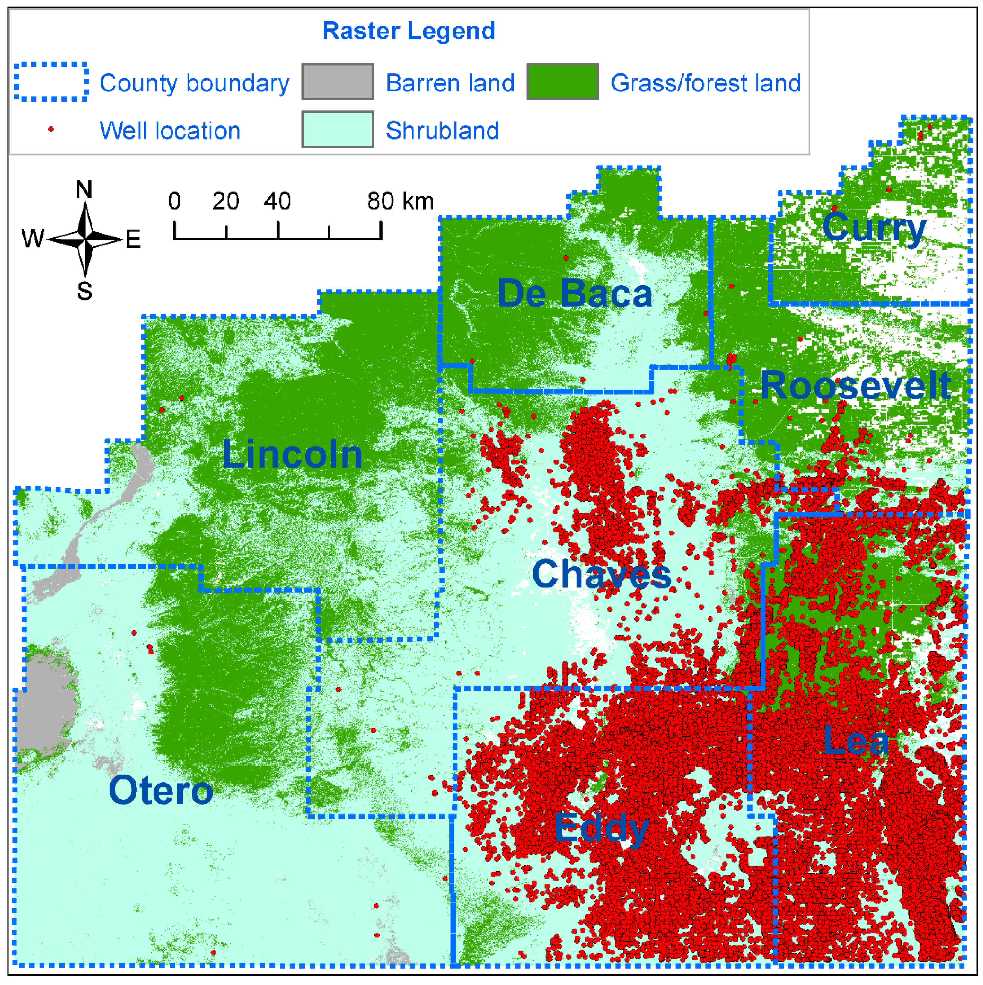
2.1. Study Area

The study area covers eight counties in southeastern New Mexico that overlap with the most productive shale formation of the Permian Basin (i.e., the Delaware sub-basin and part of the Central sub-basin). Figure 2 shows the extent of the study area. The well locations suggest that the data sample mainly comes from four counties: Chaves, Roosevelt, Eddy, and Lea. Based on some estimates (e.g., [16]), the area produces over 20% of the total output in the entire Permian Basin (40–50 counties altogether). The exorbitant intensity of production in the region leads to concerns on land cover health and other environmental issues. Figure 2 also illustrates the major vegetation covers that this study investigates. The main land cover in the active production area is shrubland surrounded by grass/forest land in the east and the north. Patches of barren land exist. Agricultural lands and developed areas (likely including drilling pads and main roads) are removed from this study to focus only on the natural vegetation cover. Agricultural lands (mostly irrigated cropland) can be found on the eastern edge of the study area. Chaves County contains a large developed area (Roswell, NM, USA).

2.2. Empirical Method

Change of land cover is a spatial-temporal process driven by multiple factors. Most of the existing studies of Southwest land cover focus mainly on change monitoring and climatic factors [34]. This study deploys a multivariate regression framework, specifically, a two-way (spatial and temporal) fixed effects panel (longitudinal) data model, to assess the impact of shale energy production on shrubland and grassland/pasture in the Permian Basin region while controlling for climatic factors. The dependent variable (P) is the percentage of the respective land cover. Independent variables include one-year lagged annual energy production (Oil) as an indicator of the magnitude of disturbance, parcel-level growing season average monthly precipitation (PPT) and temperature (Tmean). Because P is between 0 and 100%, it cannot be the dependent variable in a linear regression model directly. Instead, we apply a logistic transformation and estimate a proportional regression model [35]. In the transformed model, the dependent variable becomes the logit (log-odds) of P. Specifically, we estimate the following regression model ($i$ and $t$ are the indices for land parcel and year, respectively):

$$log\left[\frac{P_{it}}{100-P_{it}}\right]={\beta }_{1}Oi{l}_{it-1}+{\mathbf{\beta }}_{2}f\left(PP{T}_{it}, Tmea{n}_{it}\right)+{\mu }_i+{\omega }_t+{\epsilon }_{it}$$

(1)

where ${\mu }_i$ represents time-invariant fixed effects to implicitly control any spatial heterogeneities unique to each parcel, and ${\omega }_t$ represents time-varying year fixed effects capturing any region-wide trends affecting the vegetation cover. ${\epsilon }_{it}$ is the error term capturing any random shocks to the vegetation cover. ${\beta }_1$ is the parameter of interest. ${\mathbf{\beta }}_2$ is the vector of parameters associated with the climatic variables. We can recover the marginal effects of these factors on P by taking an exponential transformation on both sides of Equation (1). The following analysis also explores different specifications of the energy production variable ($Oi{l}_{it-1}$). The reason for using one-year lagged energy production is to capture the delay in vegetation cover response associated with the spatial spillover impact from energy production. Note that other control variables for the intensity of local economic activities, such as employment density, are ignored. Existing studies have shown that energy production is strongly correlated with local employment in active shale development regions (e.g., [15,22]). The following analysis adopts cross-validation to determine the best specification of $f\left(·\right)$ for the climatic variables. We estimate the regression model using the ordinary least squares (OLS) method with fixed effects ${\mu }_i$ and ${\omega }_t$ explicitly included.

2.3. Land Cover Data

This study derives the land cover data from the Crop Data Layer (CDL) developed by the NASS, USDA. The data is available for New Mexico since 2008. In recent years, the CDL has been produced using satellite imageries from the Landsat 8 OLI/TIRS sensor, the Disaster Monitoring Constellation (DMC) DEIMOS-1 and UK2, the ISRO ResourceSat-2 LISS-3, and the ESA SENTINEL-2 sensors. This study uses the CDL data for several reasons: (1) The CDL data has a relatively high spatial resolution of 30 m; (2) The CDL algorithm focuses on vegetation cover in the growing season; and (3) The fact that the CDL data classifies agricultural land uses and developed area makes it easy to separate natural vegetation cover from the rest. In this study, all agricultural land uses, water bodies, and developed lands have been removed from the analysis based on the CDL classifications. It ensures that the impact of shale energy production on shrubland and grassland/pasture can be precisely estimated. One technical caveat is the possible change/update in the classification algorithm from year to year [21], as noted in the footnote of Figure 1. However, the year fixed effects ${\omega }_t$ in the model can absorb any regionwide impacts like this. It does not affect the parameter estimates.

Shrubland is the major land cover in the study area (Figure 2). It makes up more than 70% of the land cover with a significant increase during the study period (2008–2017). Forest land and grassland/pasture only make up a little over 20% of the land cover. As Figure 1a shows, there is a significant decrease in grassland/pasture accompanied by a slight decline in wetlands (less than 0.1%) and forest land. Meanwhile, there is a noticeable increase in developed land, which likely reflects the increase in direct land use associated with shale energy development activities (e.g., drilling pads, storage facilities, access roads, and pipelines). An alternative argument is that population growth may have been driving the increase in developed areas. However, the region’s population has been stagnating in the last decade. For instance, Chaves County’s population has been around 65,000 since 2010 according to the US Census. It has even started showing a tendency of decline. Figure S1 in the Supplementary Materials shows the proportions of land cover for the entire eight-county region. The trends of vegetation cover change are very similar. Note that the statistics in Figure S1 do not necessarily represent the land cover distribution and dynamics of the core study area. There are only a handful of wells located in counties outside the core study area (Otero, Lincoln, De Baca, and Curry; Figure 2).

To focus on shrubland and grassland/pasture in the region, we first remove all farmlands, developed areas, water bodies, and other land covers. We then aggregate the remaining pixels to the 4 × 4 km PRISM climate data grid by computing the respective land cover percentages. Figure 3 illustrates one 4 × 4 km PRISM cell centered around coordinates [32°52′30″N, 104°5′2.4″W]. The aggregation of the land cover data has several benefits for empirical analysis. First, the well locations are not random across space. Due to constraints from land ownership, oil and gas wells tend to cluster spatially. Aggregating data at the PRISM grid level can smooth out sparse observations and outliers. Besides, all climatic variables are measured at the PRISM resolution. It reveals little further information by estimating a model at the CDL resolution [3]. The regression analysis excludes all PRISM cells with no oil or gas well.

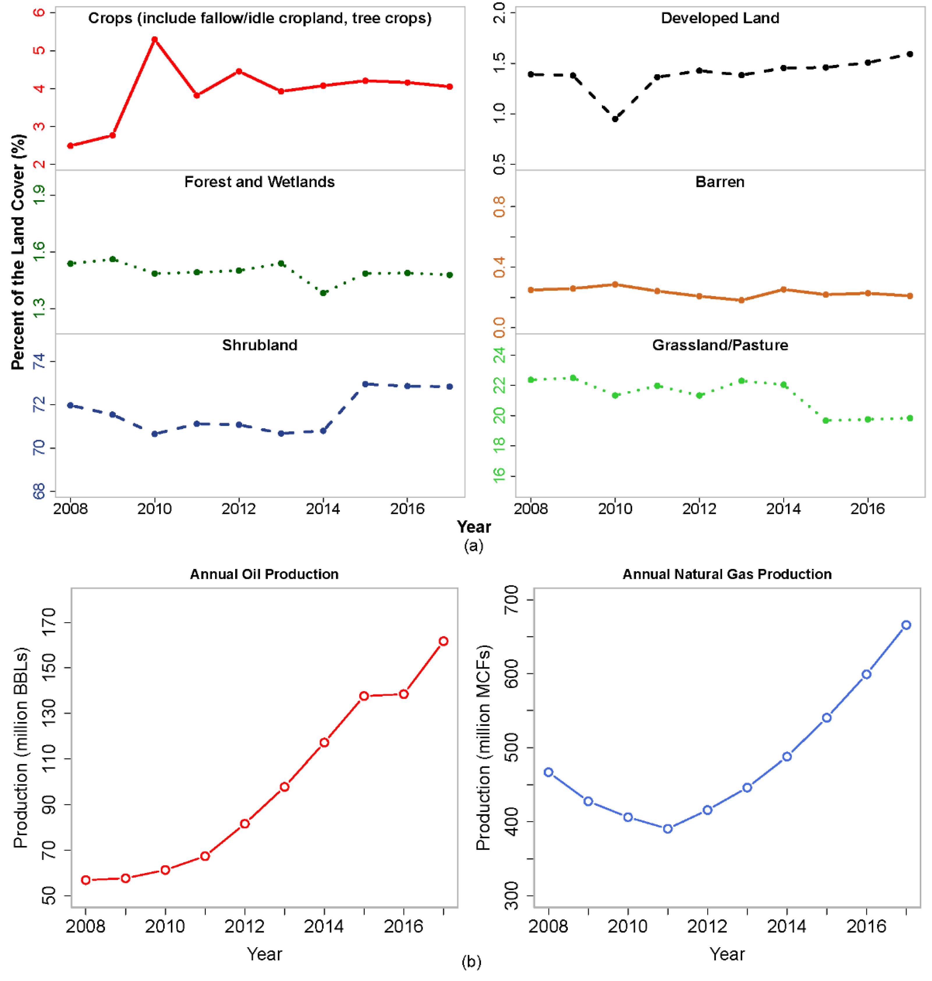
2.4. Oil and Natural Gas Production Data

The well-level annual oil and natural gas production data (including coordinates for each well) used in this study have been collected by the Petroleum Recovery Research Center at New Mexico Tech. Like other variables, we aggregate the oil and gas production data to the 4 × 4 km PRISM cell. The data reporting system records oil production (crude oil and condensate) and natural gas production (natural gas and casinghead gas). Considering the potential interaction between oil and natural gas in the production processes, we have two alternative specifications for shale energy production volume: (1) the total oil production only, given that oil production dominates shale energy production in the Permian Basin; (2) oil + gas (converted to oil-equivalent), so that it counts all energy outputs. This study uses the standard energy unit conversion factor recommended by the Society of Petroleum Engineers (SPE) and the US Energy Information Administration (EIA): one MCF natural gas ≈ 0.18 BBL (barrel of oil) oil. All of the necessary GIS shapefiles come from the US Census.

2.5. Climatic Data

The climatic variables (average monthly precipitation and temperature) used in the empirical model come from the PRISM data developed by Oregon State University. The data is commonly used for agricultural and environmental studies across the US. As part of the desert Southwest, the Permian Basin region has a relatively long growing season. Therefore, this study chooses a 10-month growing season from February to November. We compute the average monthly precipitation (PPT) and the average monthly temperature (Tmean) as the average of the monthly means reported by PRISM within the growing season. Table S1 presents summary statistics for all variables.

3. Results and Discussion

This study aims at assessing the impact of shale energy development on local shrubland and grassland/pasture. We rely on the panel (longitudinal) nature of the remote sensing data—almost 1300 cross-sectional parcels of land (PRISM cells, Table S1) being observed annually for ten years. More importantly, the panel data allows us to control for unobservable spatial heterogeneities through parcel fixed effects. Shale energy development usually goes through several stages. We can divide it into three: establishing, established, and depleting stage. Previous studies suggest that most of the disturbances on land cover happen in the early stage of shale development (e.g., [36]). It is intuitive as a lot of drilling and construction activities take place in the establishing stage. The shale energy development in the Permian Basin has experienced rapid growth in the past decade. Our 10-year study period (2008–2017) can be considered the early stage. Before 2008, the (conventional) oil and gas production in the Permian Basin was flat, as documented in other studies (e.g., [16]).

Table 1. The estimated impacts of shale energy development on shrubland (%).

Regression Variables	Model Specifications (Different Shale Production Variable)
	(1)	(2)	(3)
Oil only (million BBLs)	−2.69 (0.0000)
Oil + gas (million BBLs)		−1.89 (0.0000)
Number of oil/gas wells			−0.05 (0.0000)
PPT (cm)	1.46 (0.0000)	1.43 (0.0000)	1.47 (0.0000)
PPT^2	−0.21 (0.0000)	−0.20 (0.0000)	−0.21 (0.0000)
Tmean (°C)	2.93 (0.0639)	2.86 (0.0725)	3.02 (0.0538)
Tmean^2	0.09 (0.0739)	0.09 (0.0657)	0.09 (0.0827)
R2	0.9487	0.9488	0.9489
Study period	2008–2017

Note: (1) All estimated impacts are converted back to the unit of the dependent variable—percentage. (2) p-values are reported in the parentheses.

and

Table 2. The estimated impacts of shale energy development on grassland/pasture (%).

Regression Variables	Model Specifications (Different Shale Production Variable)
	(1)	(2)	(3)
Oil only (Million BBLs)	−0.15 (0.0009)
Oil + gas (Million BBLs)		−0.07 (0.0383)
Number of oil/gas wells			−0.00 (0.2892)
PPT (cm)	−0.17 (0.0000)	−0.17 (0.0000)	−0.17 (0.0000)
PPT^2	0.04 (0.0000)	0.04 (0.0000)	0.04 (0.0000)
Tmean (°C)	−0.07 (0.7222)	−0.06 (0.7571)	−0.04 (0.8554)
Tmean^2	−0.01 (0.0106)	−0.01 (0.0086)	−0.02 (0.0051)
R2	0.8787	0.8786	0.8786
Study period	2008–2017

Note: (1) All estimated impacts are converted back to the unit of the dependent variable—percentage. (2) p-values are reported in the parentheses.

report the estimated impacts of shale energy development on shrubland and grassland/pasture, respectively. It is worth noting three things. First, we consider three specifications of shale production for each vegetative cover. Specifications (1), (2), and (3) correspond to oil production only, oil and gas production, and the number of oil/gas wells, respectively. Second, all coefficient estimates are in the unit of the original dependent variable (%). Lastly, the year and parcel fixed effects are suppressed to conserve space. We explore their policy and management implications in the next section.

Overall, we can draw three key observations across the results. First, shale oil and gas production has statistically significant impacts on both shrubland and grassland/pasture. The effects are moderate in terms of their magnitudes. Second, the impact on the vegetation cover is more strongly associated with the hydrocarbon production volume, less with the number of oil/gas wells. It is reasonable as the impacts of drilling and completing a well last only for a short period (e.g., 1–2 years). It also suggests that hydrocarbon transportation (e.g., pipeline transport and trucking) affects the vegetation covers more. Third, between shrubland and grassland/pasture, the impact on shrubland is more pronounced in terms of its magnitude. The dominance of shrubland to other vegetation covers likely explains the result. It is also worth noting that, on average, oil production has more impact than natural gas production, as suggested by the difference between specifications (1) and (2). However, the production of oil and gas are not always separate. The same well can produce both oil and natural gas.

Specifically, the estimate −2.69 in Table 1 implies that the share of shrubland decreases by 2.69% for every one million BBLs additional oil production. Each PRISM cell is 16 km². On average, that is a 1% decline for every 23,234 BBLs additional oil production per km² and year. Similarly, the estimate −1.89 implies a 1% decline in shrubland share for every 33,069 BBLs additional hydrocarbon (oil + gas) production per km² and year. It is worth noting that natural gas production has a smaller ecological footprint because natural gas production is mostly pipeline-transported. We can interpret the impacts on grassland/pasture (Table 2) in the same way. The estimated effects on grassland/pasture are much smaller compared to shrubland. The estimate −0.15 implies a 1% decline in grassland/pasture share for every 416,667 BBLs additional oil production per km² and year. The estimate −0.07 implies a 1% decline in grassland/pasture share for every 892,857 BBLs additional hydrocarbon production per km² and year. The study region’s scarce grassland/pasture explains its relative unresponsiveness.

Although the climatic variables only serve as control variables, it is worth noting that the estimated impacts of temperature and precipitation are consistent with the literature. Overall, the average precipitation has positive but nonlinear effects on both shrubland and grassland/pasture. The average temperature has a positive impact on shrubland but a negative impact on grassland/pasture. The negative temperature effect on grassland/pasture is robust across model specifications. It is consistent with the literature on climate-change-driven woody plant encroachment in the Southwest [19,37,38]. It is also clear that the climate impact on shrubland is dominant to grassland/pasture.

A technical question left is the function form $f\left(·\right)$ for climatic variables. We have adopted the quadratic form for analyses presented in Table 1 and Table 2. The quadratic form is the best based on a cross-validation comparison of eight specifications. The literature also commonly adopts the quadratic form. Table S2 documents all candidate specifications and their mean square errors (MSEs) from 10-fold cross-validation. The best two specifications are (1) linear PPT and quadratic Tmean and (2) quadratic PPT and quadratic Tmean. They are consistent across different dependent variables and shale production variables. Tables S3 and S4 report the regression results with the specification of linear PPT and quadratic Tmean. The new estimated impacts of shale energy production on shrubland and grassland/pasture are qualitatively consistent with those in Table 1 and Table 2. There is also little quantitative change.

One caveat to note here is the potential measurement errors in the climatic data. Observational weather data (i.e., weather stations) are spatially uneven throughout the Southwest, especially in rural areas like the Permian Basin region. Model-generated climatic data usually fill the gap. However, they may not capture intraseason fluctuations in weather accurately. These potential measurement errors can affect the estimates of climatic variables. Still, they only serve as control variables. Arguably, shale energy production is independent of climatic variability and free of measurement errors. Therefore, the parameter estimates of interest—the impacts of shale energy production on vegetation cover—should be reliable.

4. Policy and Management Implications

The environmental impact of shale energy development concerns vegetation cover, (surface and ground) water quality, wildlife, etc. These issues often interconnect in the given spatial-temporal context. The current study focuses on vegetation cover that plays an essential role in the ecosystem. Besides, various environmental issues can appear or become dominant at different stages of shale energy development. It suggests that environmental policy/regulation should have adaptive and dynamic goals. For instance, produced water has become another major environmental issue in the Permian Basin recently. One possible reuse of treated produced water is to release it into the ecosystem. In that case, we need to integratively assess the shale development impact on vegetation cover and the ecosystem service value added from reusing produced water.

Specific to each of the impacts, for instance, we can observe the impact on vegetation cover. However, the groundwater quality impact may not be easy to detect without professional knowledge and testing. Another factor that often affects policy efficacy is the cost of monitoring. We can monitor vegetation cover with remote sensing data and aerial imagery, which may not work for water quality. For water quality monitoring, frequent testing of water samples is much more expensive. In many situations, including the Permian Basin, researchers and regulatory agencies often rely on voluntary data monitoring and reporting. A similar cost constraint applies to assessing the impact on wildlife. Wildlife requires more expensive field data recording due to their mobility. They are susceptible to both point contamination (e.g., an open storage tank of produced water) and nonpoint contamination (e.g., surface water pollution due to ground and surface water interactions) associated with shale development. Despite the complexities in monitoring and assessing the environmental impacts, understanding the temporal dynamics of their relative importance and dominance can improve policy efficacy in managing the environmental impacts of shale development.

Another implication to elaborate on is that natural gas production tends to have a smaller environmental impact on vegetation cover. How generalizable is this result across different contexts? The literature suggests that it is region-dependent. In the Marcellus Shale region, for example, where natural gas dominates shale energy production, the literature finds a significant impact on both interior and edge forests (e.g., [27]). A study for the US Department of the Interior shows that each horizontal shale gas well occupies on average 6.9 acres of land in the Fayetteville Shale of Arkansas [39]. That is a significant impact on land cover. It is worth noting that most of these estimates do not necessarily distinguish between land directly used by the operations (e.g., drilling pads and access roads) and land affected through the spatial spillover effects (e.g., accidental spills and temporary storage). In general, it seems that the severity of the environmental impact depends less on the difference between oil and natural gas production. It is more a matter of the magnitude of the hydrocarbon production activities. Accidental spills of produced water can cause the death/decline of trees due to its high salinity [9]. It is irrelevant whether the produced water comes from oil or gas fields.

This study can shed light on another policy-relevant question of why understanding the spatial-temporal dynamics is important. Spatial-temporal dynamics are a common feature of the ecosystem and its components such as the woody plant encroachment process, invasive species, interaction between ground and surface waters, etc. Oftentimes, solving one environmental issue is not enough. It is particularly true with shale energy development. To protect the environment, and minimize the impact on the ecosystem, integrated system-wide assessment and management strategies are necessary [7,40,41]. Exploring the spatial-temporal dynamics provides a basic framework to incorporate both biophysical factors and socio-economic factors. It can also provide guidance for adaptive environmental planning. The panel data regression framework that we adopted is commonly used in social behavior studies and some fields of environmental studies (e.g., climate change). With the increasing availability of remote sensing data and improving resolution, the method can find great uses in analyzing the land-water-energy nexus as part of the growing shale energy development in the coming decades.

A technical convenience in deriving policy implications from a panel data model is the associated fixed effects. To explicitly identify other key policy parameters, the model implicitly controls time-invariant heterogeneities (e.g., parcel-level fixed effects) and regionwide trends (e.g., year fixed effects). However, these fixed effects are impossible to decompose in the given model framework. It limits us from deriving specific policy implications out of them. Still, it is worth noting that other factors, though not of interest to this study, may impose a spatial spillover effect on vegetation cover as well. The impact of urban development driven by new economic opportunities is a good example. It can be captured as part of the regionwide trends because urban expansion means more than just housing development. It also implies more roads and traffic, higher demand for outdoor recreational activities, and so on. On top of climate change, several studies have confirmed that urban development is another main change in the background that affects vegetation cover and wildlife [36,42,43]. Those areas going through urban expansion sometimes are the same areas of active shale energy development. It is particularly true when shale energy development brings not only substantial short-term but also medium-to-long-term economic benefits (e.g., emerging new industries). One example is Midland, TX, a city in the middle of the Permian Basin. According to the US Census, the population of Midland grew by 30% between 2007 and 2016. The growth corresponded to the decade of rapid shale production growth in the Basin. Compared to other small and medium cities in western Texas and southeastern New Mexico, Midland’s urban expansion was significant. Although the potential environmental impact of urban development is not necessarily near oil and gas operations, they are usually within the same region (e.g., in the sense of a commuting zone).

5. Concluding Remarks

This study contributes to the literature one of the first integrated spatial-temporal analyses of shale energy development’s impacts on rangelands. We take advantage of the remote sensing data’s panel (longitudinal) nature to control unobserved spatial heterogeneities and regionwide trends. We show that shale development had moderate negative but statistically significant impacts on shrubland and grassland/pasture. The effect is more strongly associated with the hydrocarbon production volume, less with the number of oil and gas wells drilled. We also show that the impact of shale production on land cover varies by vegetation cover type. Between shrubland and grassland/pasture, the effect on shrubland is more pronounced in terms of magnitude. Specifically, the shrubland share on average declines 1% for every 23,234 BBLs additional oil production per km² and year. The grassland/pasture share on average declines 1% for every 416,667 BBLs additional oil production per km² and year. We obtain qualitatively consistent estimates with alternative measures of shale production. To put the estimated effects in the regional context, we calculate an aggregate impact of oil production during the ten-year study period. The ten years produced roughly 1000 million BBLs of oil in the core area of the study region (Chaves, Eddy, Lea, Roosevelt, ~44,000 km², Figure 2). The estimates above imply that the regional shrubland share was reduced by 0.98% (1000/44000/0.023234), and the regional grassland/pasture share was reduced by 0.05% (1000/44000/0.41667), over the period. In other words, if without oil and gas production, the shrubland share could be 0.98% higher, and the grassland/pasture share could be 0.05% higher. It is worth noting that our assessment captures only the first decade of shale development in the Permian Basin. As the infrastructure and wells start aging, other environmental issues like water contamination and human-induced disasters (e.g., land subsidence and airquakes) may emerge. For instance, water issues associated with testing and inject wells impose an increasing impact on the ecosystem [32].

Overall, shale development-induced environment issues on land use change, vegetation cover, and surface water quality have been relatively well-studied in the literature. At the same time, at least two other environmental issues need more research effort. One is the sequential impact on wildlife due to vegetation degradation and habitat loss. Several studies have raised such a concern [5,29,44]. However, field-level data on wildlife demographics and movement are usually expensive to collect, which is the major constraint for research in this direction. Low-altitude remote sensing is a potential solution to this problem [45,46]. By combining low-altitude remote sensing data and integrated spatial-temporal analysis, we should be able to provide a reliable assessment of the wildlife impact and shed light on policymaking.

Another issue is groundwater contamination and human-induced earthquakes (and airquakes). Most of these problems relate to disturbed underground geologic structures and geohydrology. In the Permian Basin, unconventional horizontal wells have a typical PWOR (produced water to oil ratio) of 3 [18]. Most of the produced water ends up being reinjected back into the ground, with only less than 5% of it reused in hydraulic fracturing [47]. New regulatory and policy efforts in New Mexico have emerged recently to address this environmental issue as an economic opportunity [48]. Rigorous research is still necessary to establish the scientific foundation and engineering framework in dealing with produced water as the long-term consequences of current practices (e.g., reinjecting) are unknown. Shale-development-induced earthquakes have been reported in several places around the world (e.g., [49,50]. A few studies have already tapped into this issue [51,52]. Much more is needed, especially those from an interdisciplinary perspective.

References

1. Goldewijk, K.K.; Ramankutty, N. Land cover change over the last three centuries due to human activities: The availability of new global data sets. GeoJournal 2004, 61, 335–344. [Google Scholar] [CrossRef]
2. Sukopp, H. Human-caused impact on preserved vegetation. Landsc. Urban Plan. 2004, 68, 347–355. [Google Scholar] [CrossRef]
3. Wang, H. Change of vegetation cover in the US–Mexico border region: Illegal activities or climatic variability? Environ. Res. Lett. 2019, 14, 054012. [Google Scholar] [CrossRef]
4. Allred, B.W.; Smith, W.K.; Twidwell, D.; Haggerty, J.H.; Running, S.W.; Naugle, D.E.; Fuhlendorf, S.D. Ecosystem services lost to oil and gas in North America. Science 2015, 348, 401–402. [Google Scholar] [CrossRef] [Green Version]
5. Northrup, J.M.; Wittemyer, G. Characterising the impacts of emerging energy development on wildlife, with an eye towards mitigation. Ecol. Lett. 2013, 16, 112–125. [Google Scholar] [CrossRef] [PubMed]
6. Jacquet, J.B. Review of risks to communities from shale energy development. Environ. Sci. Technol. 2014, 48, 8321–8333. [Google Scholar] [CrossRef] [PubMed]
7. Kreuter, U.P.; Iwaasa, A.D.; Theodori, G.L.; Ansley, R.J.; Jackson, R.B.; Fraser, L.H.; Naeth, M.A.; McGillivray, S.; Moya, E.G. State of knowledge about energy development impacts on North American rangelands: An integrative approach. J. Environ. Manag. 2016, 180, 1–9. [Google Scholar] [CrossRef]
8. Partridge, T.; Thomas, M.; Harthorn, B.H.; Pidgeon, N.; Hasell, A.; Stevenson, L.; Enders, C. Seeing futures now: Emergent US and UK views on shale development, climate change and energy systems. Glob. Environ. Chang. 2017, 42, 1–12. [Google Scholar] [CrossRef] [Green Version]
9. McBroom, M.; Thomas, T.; Zhang, Y. Soil erosion and surface water quality impacts of natural gas development in east Texas, USA. Water 2012, 4, 944–958. [Google Scholar] [CrossRef] [Green Version]
10. Fontenot, B.E.; Hunt, L.R.; Hildenbrand, Z.L.; Carlton Jr, D.D.; Oka, H.; Walton, J.L.; Hopkins, D.; Osorio, A.; Bjorndal, B.; Hu, Q.H.; et al. An evaluation of water quality in private drinking water wells near natural gas extraction sites in the Barnett Shale formation. Environ. Sci. Technol. 2013, 47, 10032–10040. [Google Scholar] [CrossRef]
11. Olmstead, S.M.; Muehlenbachs, L.A.; Shih, J.S.; Chu, Z.; Krupnick, A.J. Shale gas development impacts on surface water quality in Pennsylvania. Proc. Natl. Acad. Sci. USA 2013, 110, 4962–4967. [Google Scholar] [CrossRef] [Green Version]
12. Vidic, R.D.; Brantley, S.L.; Vandenbossche, J.M.; Yoxtheimer, D.; Abad, J.D. Impact of shale gas development on regional water quality. Science 2013, 340, 1235009. [Google Scholar] [CrossRef] [Green Version]
13. MacDonald, G.M. Water, climate change, and sustainability in the southwest. Proc. Natl. Acad. Sci. USA 2010, 107, 21256–21262. [Google Scholar] [CrossRef] [Green Version]
14. Pascale, S.; Boos, W.R.; Bordoni, S.; Delworth, T.L.; Kapnick, S.B.; Murakami, H.; Vecchi, G.A.; Zhang, W. Weakening of the North American monsoon with global warming. Nat. Clim. Chang. 2017, 7, 806–812. [Google Scholar] [CrossRef]
15. Lee, J. The regional economic impact of oil and gas extraction in Texas. Energy Policy 2015, 87, 60–71. [Google Scholar] [CrossRef]
16. Wang, H. The economic impact of oil and gas development in the Permian Basin: Local and spillover effects. Resour. Policy 2020, 66, 101599. [Google Scholar] [CrossRef]
17. James, A.; Smith, B. There will be blood: Crime rates in shale-rich US counties. J. Environ. Econ. Manag. 2017, 84, 125–152. [Google Scholar] [CrossRef] [Green Version]
18. Scanlon, B.R.; Reedy, R.C.; Male, F.; Walsh, M. Water issues related to transitioning from conventional to unconventional oil production in the Permian Basin. Environ. Sci. Technol. 2017, 51, 10903–10912. [Google Scholar] [CrossRef]
19. Grover, H.D.; Musick, H.B. Shrubland encroachment in southern New Mexico, USA: An analysis of desertification processes in the American Southwest. Clim. Chang. 1990, 17, 305–330. [Google Scholar] [CrossRef]
20. Beschta, R.L.; Donahue, D.L.; DellaSala, D.A.; Rhodes, J.J.; Karr, J.R.; O’Brien, M.H.; Fleischner, T.L.; Williams, C.D. Adapting to climate change on western public lands: Addressing the ecological effects of domestic, wild, and feral ungulates. Environ. Manag. 2013, 51, 474–491. [Google Scholar] [CrossRef] [PubMed]
21. Johnson, D.M. A 2010 map estimate of annually tilled cropland within the conterminous United States. Agric. Syst. 2013, 114, 95–105. [Google Scholar] [CrossRef]
22. Feyrer, J.; Mansur, E.T.; Sacerdote, B. Geographic dispersion of economic shocks: Evidence from the fracking revolution. Am. Econ. Rev. 2017, 107, 1313–1334. [Google Scholar] [CrossRef] [Green Version]
23. van Auken, O.W. Causes and consequences of woody plant encroachment into western North American grasslands. J. Environ. Manag. 2009, 90, 2931–2942. [Google Scholar] [CrossRef] [PubMed]
24. Moran, M.D.; Cox, A.B.; Wells, R.L.; Benichou, C.C.; McClung, M.R. Habitat loss and modification due to gas development in the Fayetteville Shale. Environ. Manag. 2015, 55, 1276–1284. [Google Scholar] [CrossRef]
25. Johnstone, J.F.; Kokelj, S.V. Environmental conditions and vegetation recovery at abandoned drilling mud sumps in the Mackenzie Delta region, Northwest Territories, Canada. Arctic 2008, 61, 199–211. [Google Scholar] [CrossRef] [Green Version]
26. Nash, M.; Wickham, J.; Christensen, J.; Wade, T. Changes in landscape greenness and climatic factors over 25 years (1989–2013) in the USA. Remote Sens. 2017, 9, 295. [Google Scholar] [CrossRef] [PubMed] [Green Version]
27. Slonecker, E.T.; Milheim, L.E.; Roig-Silva, C.M.; Malizia, A.R.; Marr, D.A.; Fisher, G.B. Landscape Consequences of Natural Gas Extraction in Bradford and Washington Counties, Pennsylvania; US Geological Survey Open-File Report 2012–1154; U.S. Geological Survey: Reston, VA, USA, 2012. [Google Scholar]
28. Drohan, P.J.; Brittingham, M.; Bishop, J.; Yoder, K. Early trends in land cover change and forest fragmentation due to shale-gas development in Pennsylvania: A potential outcome for the Northcentral Appalachians. Environ. Manag. 2012, 49, 1061–1075. [Google Scholar] [CrossRef]
29. Thomas, E.H.; Brittingham, M.C.; Stoleson, S.H. Conventional oil and gas development alters forest songbird communities. J. Wildl. Manag. 2014, 78, 293–306. [Google Scholar] [CrossRef]
30. Langlois, L.A.; Drohan, P.J.; Brittingham, M.C. Linear infrastructure drives habitat conversion and forest fragmentation associated with Marcellus shale gas development in a forested landscape. J. Environ. Manag. 2017, 197, 167–176. [Google Scholar] [CrossRef] [PubMed] [Green Version]
31. Pattison, C.A.; Quinn, M.S.; Dale, P.; Catterall, C.P. The landscape impact of linear seismic clearings for oil and gas development in boreal forest. Northwest Sci. 2016, 90, 340–355. [Google Scholar] [CrossRef]
32. Preston, T.M.; Kim, K. Land cover changes associated with recent energy development in the Williston Basin; Northern Great Plains, USA. Sci. Total Environ. 2016, 566, 1511–1518. [Google Scholar] [CrossRef]
33. Jones, I.L.; Bull, J.W.; Milner-Gulland, E.J.; Esipov, A.V.; Suttle, K.B. Quantifying habitat impacts of natural gas infrastructure to facilitate biodiversity offsetting. Ecol. Evol. 2014, 4, 79–90. [Google Scholar] [CrossRef] [PubMed]
34. Lam, D.K.; Remmel, T.K.; Drezner, T.D. Tracking desertification in California using remote sensing: A sand dune encroachment approach. Remote Sens. 2011, 3, 1–13. [Google Scholar] [CrossRef] [Green Version]
35. Papke, L.E.; Wooldridge, J.M. Econometric methods for fractional response variables with an application to 401 (k) plan participation rates. J. Appl. Econom. 1996, 11, 619–632. [Google Scholar] [CrossRef] [Green Version]
36. Braun, C.E.; Oedekoven, O.O.; Aldridge, C.L. Oil and gas development in western North America: Effects on sagebrush steppe avifauna with particular emphasis on sage-grouse. In Proceedings of the 67th North American Wildlife and Natural Resources Conference, Wildlife Management Institute, Washington, DC, USA, 3–7 April 2002. [Google Scholar]
37. Brown, J.R.; Archer, S. Shrub invasion of grassland: Recruitment is continuous and not regulated by herbaceous biomass or density. Ecology 1999, 80, 2385–2396. [Google Scholar] [CrossRef]
38. Briggs, J.M.; Schaafsma, H.; Trenkov, D. Woody vegetation expansion in a desert grassland: Prehistoric human impact? J. Arid Environ. 2007, 69, 458–472. [Google Scholar] [CrossRef]
39. Arthur, J.D.; Langhus, B.; Alleman, D. An Overview of Modern Shale Gas Development in the United States. A Report by All Consulting. 2008. Available online: http://www.ourenergypolicy.org/wp-content/uploads/2013/10/ALLShaleOverviewFINAL.pdf (accessed on 8 October 2019).
40. Meng, Q. The impacts of fracking on the environment: A total environmental study paradigm. Sci. Total Environ. 2017, 580, 953–957. [Google Scholar] [CrossRef] [PubMed]
41. McClung, M.R.; Moran, M.D. Understanding and mitigating impacts of unconventional oil and gas development on land-use and ecosystem services in the US. Curr. Opin. Environ. Sci. Health 2018, 3, 19–26. [Google Scholar] [CrossRef]
42. Pierre, J.P.; Wolaver, B.D.; Labay, B.J.; LaDuc, T.J.; Duran, C.M.; Ryberg, W.A.; Hibbitts, T.J.; Andrews, J.R. Comparison of recent oil and gas, wind energy, and other anthropogenic landscape alteration factors in Texas through 2014. Environ. Manag. 2018, 61, 805–818. [Google Scholar] [CrossRef]
43. Mubako, S.; Belhaj, O.; Heyman, J.; Hargrove, W.; Reyes, C. Monitoring of land use/land-cover changes in the arid transboundary Middle Rio Grande Basin using remote sensing. Remote Sens. 2018, 10, 2005. [Google Scholar] [CrossRef] [Green Version]
44. Kiviat, E. Risks to biodiversity from hydraulic fracturing for natural gas in the Marcellus and Utica shales. Ann. N. Y. Acad. Sci. 2013, 1286, 1–14. [Google Scholar] [CrossRef]
45. Jones IV, G.P.; Pearlstine, L.G.; Percival, H.F. An assessment of small unmanned aerial vehicles for wildlife research. Wildl. Soc. Bull. 2006, 34, 750–758. [Google Scholar] [CrossRef]
46. Watts, A.C.; Perry, J.H.; Smith, S.E.; Burgess, M.A.; Wilkinson, B.E.; Szantoi, Z.; Ifju, P.G.; Percival, H.F. Small unmanned aircraft systems for low-altitude aerial surveys. J. Wildl. Manag. 2010, 74, 1614–1619. [Google Scholar] [CrossRef]
47. Scanlon, B.R.; Reedy, R.C.; Nicot, J.P. Will water scarcity in semiarid regions limit hydraulic fracturing of shale plays? Environ. Res. Lett. 2014, 9, 124011. [Google Scholar] [CrossRef] [Green Version]
48. Davis, T. State Joins NMSU to Research Produced Water. 2019. Available online: https://www.abqjournal.com/1365495/state-joins-nmsu-to-research-produced-water-ex-aim-is-to-turn-a-waste-product-into-a-commodity.html (accessed on 8 October 2019).
49. Boffey, D. Gas Field Earthquakes Put Netherlands’ Biggest Firms on Extraction Notice. 2018. Available online: https://www.theguardian.com/environment/2018/jan/23/gas-field-earthquakes-put-netherlands-biggest-firms-on-extraction-notice (accessed on 8 October 2019).
50. Gernon, T. Earthquakes from the Oil and Gas Industry Are Plaguing Oklahoma here’s a Way to Reduce Them. 2018. Available online: https://theconversation.com/earthquakes-from-the-oil-and-gas-industry-are-plaguing-oklahoma-heres-a-way-to-reduce-them-91044 (accessed on 8 October 2019).
51. Koster, H.R.; Van Ommeren, J. A shaky business: Natural gas extraction, earthquakes and house prices. Eur. Econ. Rev. 2015, 80, 120–139. [Google Scholar] [CrossRef]
52. Yoon, C.E.; Huang, Y.; Ellsworth, W.L.; Beroza, G.C. Seismicity during the initial stages of the Guy-Greenbrier, Arkansas, earthquake sequence. J. Geophys. Res. Solid Earth 2017, 122, 9253–9274. [Google Scholar] [CrossRef]
Figure 1. Land cover change (a) and energy production (b) in Lea and Eddy Counties, New Mexico. Data sources: (a) computed from the 30 m Crop Data Layer (CDL) by the National Agricultural Statistics Service (NASS); (b) computed from well-level data provided by the Petroleum Recovery Research Center at New Mexico Tech. Note: (1) one MCF = one thousand cubic feet; (2) The sudden decline in developed land and the corresponding jump in cropland in 2010 is likely caused by the classification algorithm that processed the CDL [21].
Remotesensing 13 00824 g001
Figure 2. Study area overlapped with recoded CDL and well locations (as of 2017). Data sources: CDL by the National Agricultural Statistics Service (NASS) and well location data from the Petroleum Recovery Research Center at New Mexico Tech. Note: plain (white) CDL pixels represent other land uses (mostly agriculture and developed land uses) being removed.
Remotesensing 13 00824 g002
Figure 3. Recoded land cover and well locations within one PRISM pixel (4 × 4 km). Data sources: CDL by the NASS and well location data from the Petroleum Recovery Research Center at New Mexico Tech. Note: plain (white) CDL pixels represent other land uses (mostly agriculture and developed land uses) being removed. The CDL raster layer is from 2010. The PRISM pixel centers around coordinates [32°52′30″N, 104°5′2.4″W] using the WGS 1984 Datum (used in Google Maps as well).
Remotesensing 13 00824 g003