DOA and Range Estimation for FDA-MIMO Radar with Sparse Bayesian Learning

Abstract

Due to grid division, the existing target localization algorithms based on sparse signal recovery for the frequency diverse array multiple-input multiple-output (FDA-MIMO) radar not only suffer from high computational complexity but also encounter significant estimation performance degradation caused by off-grid gaps. To tackle the aforementioned problems, an effective off-grid Sparse Bayesian Learning (SBL) method is proposed in this paper, which enables the calculation the direction of arrival (DOA) and range estimates. First of all, the angle-dependent component is split by reconstructing the received data and contributes to immediately extract rough DOA estimates with the root SBL algorithm, which, subsequently, are utilized to obtain the paired rough range estimates. Furthermore, a discrete grid is constructed by the rough DOA and range estimates, and the 2D-SBL model is proposed to optimize the rough DOA and range estimates. Moreover, the expectation-maximization (EM) algorithm is utilized to update the grid points iteratively to further eliminate the errors caused by the off-grid model. Finally, theoretical analyses and numerical simulations illustrate the effectiveness and superiority of the proposed method.

1. Introduction

Target localization has been extensively researched in the past few decades, which forms a diversity of applications in navigation, radar, remote sensing, communication, and unmanned driving [1,2,3,4,5]. At present, lidar and radar play important roles in target localization. Lidar uses laser pulses to scan the actual scene to achieve high-precision target localization [6,7], and the radar extracts the spatial position information of the target by receiving the reflected electromagnetic waves. Compared with lidar, radar has broader application scenarios such as at night, in rain, and in fog. Recently, multiple-input multiple-output (MIMO) radar has received extensive attention in target localization due to many potential advantages [8,9]. Different from the phased array radar, MIMO radar has higher degrees of freedom (DOFs) and spatial resolution [10,11,12,13], where multiple antennas simultaneously transmit different waveforms and receive reflected signals synchronously. Nevertheless, the MIMO radar fails to estimate the range of the target directly because its beam pointing is only related to the angle.

Frequency diverse array (FDA) is an institutional array with emerging technology [14,15,16], which has massive potential advantages in target parameter estimation. FDA can provide the angle-range related beam-pattern through small frequency increments across the transmitters, which is expected to implement joint angle and range estimation. However, ambiguous estimates [17] may be caused in FDA radar due to the direction of arrival (DOA) and range coupling in the steering vector matrix, which will result in the deterioration of estimation accuracy. Therefore, it is crucial to decouple the parameters of DOA and range to obtain unambiguous and unique parameter estimations. The authors of [18] introduced a double-pulse method to obtain DOA and range estimates by emitting pulses with zero and nonzero frequency increments. In [19], the FDA is divided into two subarrays according to different frequency increments to estimate the DOA and range. Moreover, some design strategies have utilized nonlinear frequency increments to decouple the parameters of DOA and range, such as random frequency increment [20] and logarithmic frequency increment [21].

The combination of FDA and MIMO radar is another decoupling strategy, which uses the high DOF of MIMO radar to decouple the DOA and range of FDA-MIMO radar [22,23,24,25,26]. The authors of [27] introduced a method of signal parameters via a rotational invariance technique (ESPRIT) to estimate the target parameters for FDA-MIMO radar. In [28], a unitary ESPRIT method has been introduced with low complexity that can solve the periodic ambiguity problem. Additionally, a two-dimensional multiple signal classification (2D-MUSIC) method was proposed for DOA and range estimation in FDA-MIMO radar [29]. However, the above-mentioned methods based on subspace decomposition require an accurate signal subspace or noise subspace to achieve high-resolution performance, and their performance will significantly deteriorate in the case that the snapshots are scarce or the signal-to-noise ratio (SNR) is low.

In recent years, the rapid development of sparse signal recovery (SSR) technology provides a new perspective for target localization [30,31,32]. Compared with the subspace-based methods, the SSR methods have many prominent merits, e.g., limited number of snapshots, solved correlation of signals and improved robustness to noise. In the past few decades, various SSR methods for DOA estimation have been proposed, such as $l_1$-norm optimization-based algorithm [33,34] and the sparse Bayesian learning (SBL) method [35,36,37]. Compared with the $l_1$-norm optimization-based algorithm, the SBL-based algorithm can still have good performance in the case of high SNR or a coarse sampling grid. The authors of [38] proposed the off-grid sparse Bayesian inference (OGSBI) method firstly, which can accurately describe the real observation model even in the case of a high SNR or a coarse sampling grid. The root off-grid sparse Bayesian learning (ROGSBL) algorithm has been proposed in [39], which can achieve accurate DOA estimation with a low computational burden. In order to further reduce the computational burden, the authors of [40] proposed an enhanced SBL method to achieve off-grid DOA estimation, which dynamically updates the grid points through the forgetting factor model. Moreover, sparse Bayesian learning with the mutual coupling (SBLMC) method is proposed in [41] to eliminate the mutual coupling effect between array antennas.

However, only a few target localization methods for FDA-MIMO radar adopt SSR technology except for the double-pulse $l_1$-SVD method [42]. The reason is that the SSR methods cannot be directly applied to FDA-MIMO radar for target localization due to the coupling of DOA and range. Moreover, the on-grid model adopted by the double-pulse $l_1$-SVD method cannot accurately describe the real observation model in the case of high SNR or a coarse sampling grid, which leads to degraded parameter estimation performance. Hence, in order to improve the DOA and range estimation accuracy of FDA-MIMO radar in a complexly practical environment, it is necessary to effectively tackle the problem of the off-grid gap. The off-grid SBL-based algorithm is very robust to the off-grid gap, so it provides us with a new perspective.

In this paper, an effective off-grid SBL method is proposed to achieve the DOA and range estimates. Firstly, the angle-dependent component is split by reconstructing the received data and contributes to immediately extract rough DOA estimates with the root SBL algorithm, which, subsequently, are utilized to obtain the paired rough range estimates. The decoupling strategy in this paper will damage the array aperture of the FDA-MIMO radar, so we need to further optimize the rough estimation of DOA and range. Furthermore, a discrete grid is constructed by the rough DOA and range estimates, and the 2D-SBL model is proposed to optimize the rough estimates of DOA and range. Finally, the expectation-maximization (EM) algorithm is utilized to update the grid points iteratively to further eliminate the errors caused by the off-grid model. Therefore, the proposed method has a better performance compared with the double-pulse $l_1$-SVD method [42]. Additionally, the proposed method is one of the methods in SSR, so this method has a better effect than the subspace algorithms in the case of low SNR or scarce snapshots. The main contributions of the proposed method are summarized as follows:

• The proposed method achieves DOA and range estimates of FDA-MIMO radar through SSR technology, which overcomes the shortcoming of the existing subspace algorithms. This method has a better effect than the subspace algorithms in the case of low SNR or scarce snapshots.
• We proposed a new decoupling strategy to decouple the DOA and range parameters of FDA-MIMO radar so that the SSR methods can be directly used in FDA-MIMO radar to achieve target localization. Moreover, the DOA and range estimates of the targets will be automatically matched.
• To further eliminate the adverse effects caused by the off-grid gap, we introduced a grid refinement method in the 2D-SBL framework, where the positions of grid points will be regarded as adjustable parameters and the grid points will be updated recursively. After some iterations, the updated grid points will tend to approximate the real DOA and range, so the off-grid gap can be almost eliminated.

The rest of this paper is organized as follows. In Section 2, we describe the FDA-MIMO radar model for DOA and range estimation. The proposed DOA and range estimation method with sparse Bayesian learning is presented in Section 3. In Section 4, we summarize the complexity of the proposed method and derive the CRB of the FDA-MIMO radar. Simulation results and conclusion follow in Section 5 and Section 6, respectively.

The symbols related to this paper are shown in Table 1.

Table 1. Related notation.

Notations	Definitions
lowercase bold italic letters	vectors
capital bold italic letters	matrices
${(·)}^T$	transpose operation
${(·)}^{†}$	pseudoinverse operation
${(·)}^{\ast }$	conjugate operation
${(·)}^H$	conjugate-transpose operation
$diag(·)$	diagonalization operation
$angle(·)$	extract the phase angle
$tr(·)$	trace of the matrix
∘	Hadamard product
⊙	Khatri-Rao product
⊗	Kronecker product
${\mathit{I}}_N$	identity matrix of order N
${\mathbb{C}}^{M\times P}$	$M\times P$ complex matrix set
$CN(0,q)$	Gaussian distribution with zero mean and q variance

2. Signal Model

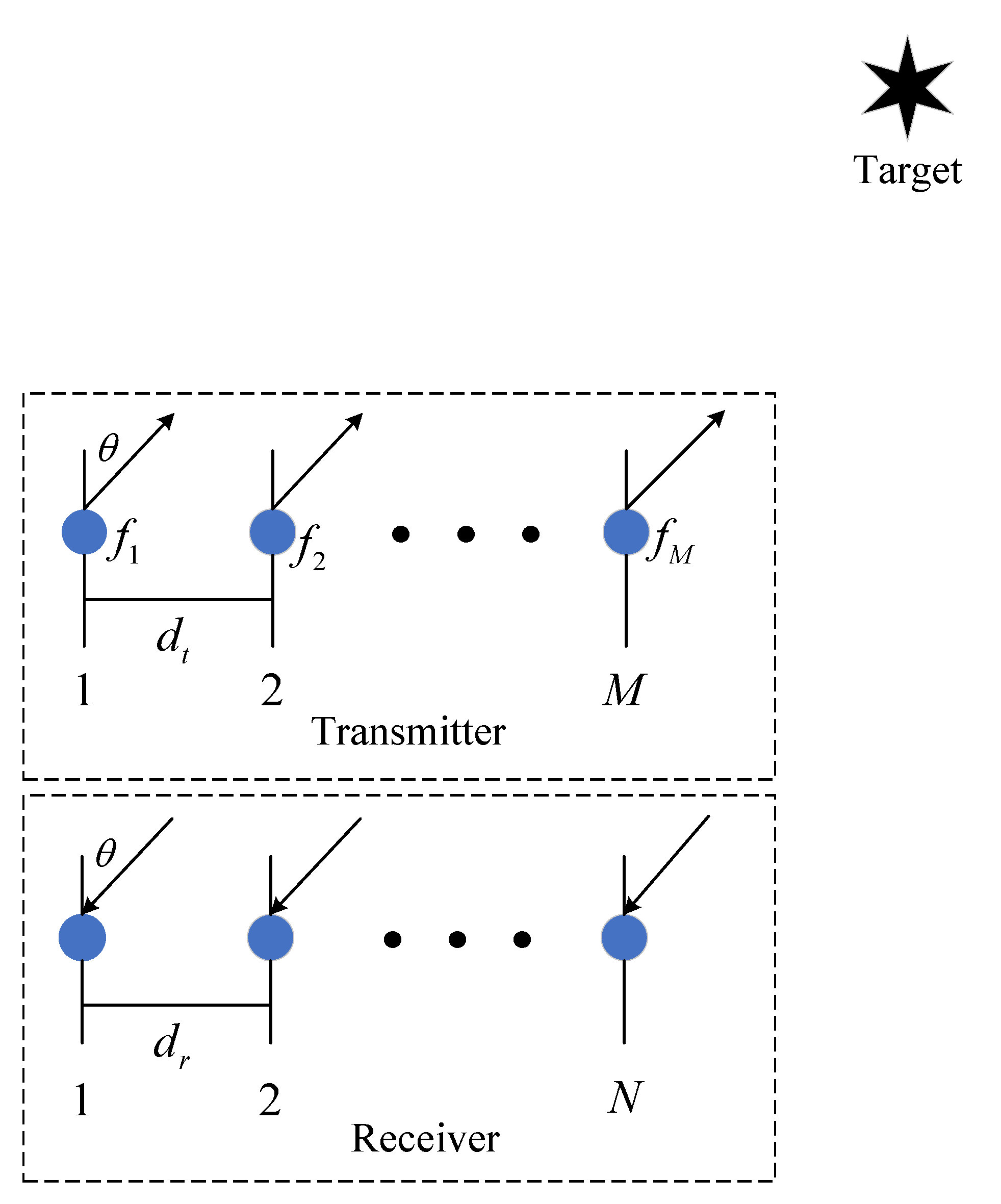
Consider a monostatic FDA-MIMO radar consisting of M transmitting antennas and N receiving antennas as shown in Figure 1. Both the transmitter and receiver are uniform linear arrays (ULAs), where the spacings between adjacent elements are denoted as $d_t$ and $d_r$, respectively. The frequency of the first antenna in the transmitter is selected as the reference frequency, and the transmitting frequency of the m-th transmitting antenna is

$$f_m=f_1+(m-1)\Delta f,m=1,2,\cdots ,M$$

(1)

where $f_1$ represents the reference frequency in the transmitter, and $\Delta f$ is the increment of the transmitting frequency of the adjacent antennas in the transmitter.

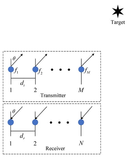
Figure 1. Monostatic FDA-MIMO radar.

The narrowband complex signal emitted by the m-th antenna in the transmitter can be expressed as

$$s_m(\widehat{t})={\varphi }_m(\widehat{t})e^{j2\pi f_m\widehat{t}},0\le \widehat{t}\le \widehat{T}$$

(2)

where ${\varphi }_m(\widehat{t})$ represents the baseband signal of the m-th antenna in the transmitter, $\widehat{T}$ denotes the duration of the radar pulse. We assume that the baseband waveforms are orthogonal to each other, and can be expressed as

$${\int }_0^{\widehat{T}}{\varphi }_m(\widehat{t}){\varphi }_n^{\ast }(\widehat{t}-\tau )e^{j2\pi \widehat{t}(m-n)\Delta f}d\widehat{t}=\left\{\begin{array}{cc}\hfill & 1,m=n,\tau =0\hfill \\ \hfill & 0,m\ne n,\forall \tau \hfill \end{array}\right.$$

(3)

Suppose there are K far-field targets whose ranges are much larger than the aperture of the FDA-MIMO radar. The output of the receiver after performing matched filtering can be expressed as

$$\mathit{x}(t)=\mathit{As}(t)+\mathit{n}(t)$$

(4)

where $\mathit{x}(t)={[x_1(t),x_2(t),\cdots ,x_{MN}(t)]}^T\in {\mathbb{C}}^{MN\times 1}$ is a received signal vector. $\mathit{s}(t)={[s_1(t),s_2(t),\dots ,s_K(t)]}^T\in {\mathbb{C}}^{K\times 1}$ and $n(t)={[n_1(t),n_2(t),\cdots ,n_{MN}(t)]}^T\in {\mathbb{C}}^{MN\times 1}$ represent signal source vector and noise vector, respectively. $\mathit{A}=[\mathit{a}({\theta }_1,r_1),\mathit{a}({\theta }_2,r_2),\dots ,$$\mathit{a}({\theta }_K,r_K)]\in {\mathbb{C}}^{MN\times K}$ is the joint transmit-receive steering matrix, and $\mathit{a}({\theta }_k,r_k)={\mathit{a}}_r({\theta }_k)\otimes {\mathit{a}}_t({\theta }_k,r_k),k=1,2,\dots ,K$. The steering vector of the transmitter and receiver can be represented by

$$\begin{array}{cc}\hfill & {\mathit{a}}_t({\theta }_k,r_k)={\left[1,e^{-j4\pi \frac{\Delta f}{c}{r}_k},\dots ,e^{-j4\pi \frac{\Delta f}{c}\left(M-1\right)r_k}\right]}^T\hfill \\ \hfill & \circ {\left[1,e^{j2\pi \frac{d_t}{\lambda }sin({\theta }_k)},\dots ,e^{j2\pi \frac{d_t}{\lambda }\left(M-1\right)sin{\theta }_k}\right]}^T\hfill \end{array}$$

(5)

$${\mathit{a}}_r({\theta }_k)={\left[1,e^{j2\pi \frac{d_r}{\lambda }sin{\theta }_k},\dots ,e^{j2\pi \frac{d_r}{\lambda }\left(N-1\right)sin{\theta }_k}\right]}^T$$

(6)

The output of matched filter via gathering T snapshots can be expressed as

$$\mathit{X}=\mathit{AS}+\mathit{N}$$

(7)

where $\mathit{X}=[\mathit{x}(1),\mathit{x}(2),\cdots ,\mathit{x}(T)]\in {\mathbb{C}}^{MN\times T}$, $\mathit{S}=[\mathit{s}(1),\mathit{s}(2),\cdots ,\mathit{s}(T)]\in {\mathbb{C}}^{K\times T}$ and $\mathit{N}=[\mathit{n}(1),\mathit{n}(2),\cdots ,\mathit{n}(T)]\in {\mathbb{C}}^{MN\times T}$.

3. DOA and Range Estimation for FDA-MIMO Radar

In this section, a sparse Bayesian learning method is proposed for DOA and range estimation of FDA-MIMO radar. Firstly, the angle-dependent component is split by reconstructing the received data and contributes to immediately extract rough DOA estimates with the root SBL algorithm, which, subsequently, are utilized to obtain the paired rough range estimates. Furthermore, a discrete grid is constructed by the rough DOA and range estimates, and the 2D-SBL model is proposed to optimize the rough estimates of DOA and range. Finally, the EM algorithm is utilized to update the grid points iteratively to further eliminate the errors caused by the off-grid model.

3.1. Decoupling the Parameters of DOA and Range

The transmit-receive steering matrix can be rewritten as [43]

$$\mathit{A}={\mathit{A}}_r\odot {\mathit{A}}_t=\left[\begin{array}{c}{\mathit{A}}_t\\ {\mathit{A}}_t{\mathit{\Phi }}_r\\ ⋮\\ {\mathit{A}}_{{}_t}{\mathit{\Phi }}_r^{N-1}\end{array}\right]$$

(8)

where ${\mathit{A}}_r=[{\mathit{a}}_r({\theta }_1),{\mathit{a}}_r({\theta }_2),\cdots ,{\mathit{a}}_r({\theta }_K)]\in {\mathbb{C}}^{N\times K}$ and ${\mathit{A}}_t=[{\mathit{a}}_t({\theta }_1,r_1),{\mathit{a}}_r({\theta }_2,r_2),\cdots ,$${\mathit{a}}_r({\theta }_K,r_K)]\in {\mathbb{C}}^{M\times K}$ are receiving steering matrix and transmitting steering matrix, respectively. ${\mathit{\Phi }}_r=diag({\varphi }_1^r,{\varphi }_2^r,\cdots ,{\varphi }_K^r)$ with the k-th element of the main diagonal denoted by ${\varphi }_k^r=e^{j2\pi \frac{f_1}{c}{d}_{r}sin({\theta }_k)}$.

A $M\ast N$ dimensional matrix $\mathit{Z}$ can be expressed as

$$\mathit{Z}=\left[\begin{array}{cccc}1& 2& \cdots & M\\ M+1& M+2& \cdots & 2M\\ ⋮& ⋮& \ddots & ⋮\\ (N-1)\ast M+1& (N-1)\ast M+2& \cdots & M\ast N\end{array}\right]$$

(9)

Then, arrange the elements of $\mathit{Z}$ in columns to form a vector $\mathit{z}=[z_1,z_2,\cdots ,z_{MN}]\in {\mathbb{C}}^{MN\times 1}$. Suppose a vector is $\mathit{w}=[w_1,w_2,\cdots ,w_{MN}]=[1,2,\cdots ,MN]\in {\mathbb{C}}^{MN\times 1}$. Combine elements at the same position in vector ${w}$ and vector ${z}$ into a number pair, where the element in ${w}$ represents the column index and the element in ${z}$ represents the row index. $\mathbf{Q}\in {\mathbb{C}}^{MN\times MN}$ is a selection matrix whose elements meet the following constraints

$$\mathbf{Q}(i,j)=\left\{\begin{array}{cc}\hfill & 1i=z_v,j=w_v\hfill \\ \hfill & 0\mathrm{else}\hfill \end{array}\right.,v=1,2,\cdots ,MN$$

(10)

A new matrix ${\mathit{X}}_Q$ is defined by

$${\mathit{X}}_Q=\mathit{QX}=\mathit{QAS}+\mathit{QN}$$

(11)

where $\mathit{B}=\mathit{QA}$

$${B}=\left[\begin{array}{c}{\mathit{A}}_r\\ {\mathit{A}}_r{\mathit{\Phi }}_t\\ ⋮\\ {\mathit{A}}_r{\mathit{\Phi }}_t^{M-1}\end{array}\right]$$

(12)

where ${\mathit{\Phi }}_t=diag({\varphi }_1^t,{\varphi }_2^t,\cdots ,{\varphi }_K^t)$, and the k-th element of the main diagonal is ${\varphi }_k^t=e^{j\frac{2\pi }{c}(d_t{f}_{1}sin({\theta }_k)-\Delta f2r_k)}$.

According to (8) and (12), the matrix ${\mathit{X}}_a$ formed by the first N rows of ${\mathit{X}}_Q$ only is angle-dependent while the matrix ${\mathit{X}}_r$ formed by the first M rows of $\mathit{X}$ contains DOA and range.

3.2. Rough DOA Estimation

To utilize the SBL method for DOA estimation, we construct the sparse representation model by [44]

$${\mathit{X}}_a={\mathit{A}}_{\overline{\theta }}{\mathit{S}}_{\overline{K}}+{\mathit{N}}_a$$

(13)

where $\overline{\mathit{\theta }}=[{\overline{\theta }}_1,{\overline{\theta }}_2,\cdots ,{\overline{\theta }}_{\overline{K}}]$ is established by sampling the spatial domain range $[-\pi /2,\pi /2]$ uniformly, where $\overline{K}\gg N>K$. ${\mathit{A}}_{\overline{\theta }}=[{\mathit{a}}_r({\overline{\theta }}_1),{\mathit{a}}_r({\overline{\theta }}_2),\cdots ,{\mathit{a}}_r({\overline{\theta }}_{\overline{K}})]\in {\mathbb{C}}^{N\times \overline{K}}$ is an over-complete dictionary and ${\mathit{a}}_r({\overline{\theta }}_{\overline{k}})={\left[1,e^{j2\pi \frac{d_r}{\lambda }sin{\overline{\theta }}_{\overline{k}}},\dots ,e^{j2\pi \frac{d_r}{\lambda }\left(N-1\right)sin{\overline{\theta }}_{\overline{k}}}\right]}^T$ with $\overline{k}=1,2,\cdots ,\overline{K}$. ${\mathit{N}}_a$ is the matrix formed by the first N rows of $\mathit{QN}$. ${\mathit{S}}_{\overline{K}}=[{\mathit{s}}_{\overline{K}}(1),{\mathit{s}}_{\overline{K}}(2),\cdots ,$${\mathit{s}}_{\overline{K}}(T)]\in {\mathbb{C}}^{\overline{K}\times T}$ is a sparse matrix, and ${\mathit{s}}_{\overline{K}}(t)={[s_1(t),s_2(t),\cdots ,s_{\overline{K}}(t)]}^T$ is a K-order sparse column vector.

It is generally assumed that Gaussian white noise ${\mathit{N}}_a$ follows the probability distribution [45]

$$p({\mathit{N}}_a\left|{\beta }_a\right.)=\underset{t=1}{\stackrel{T}{\Pi }}CN(n_a(t)\left|0\right.,{\beta }_a^{-1}{\mathit{I}}_N)$$

(14)

where ${\beta }_a={\sigma }_a^{-2}$, ${\sigma }_a^2$ represents noise power. In order to facilitate analysis and calculation, it is further assumed that ${\beta }_a$ follows an independent gamma distribution as

$$p({\beta }_a;a,b)=Gamma({\beta }_a\left|a,b\right.)$$

(15)

where $Gamma({\beta }_a\left|a,b\right.)=\Gamma {({\beta }_a)}^{-1}{b}^a{\beta }_a^{a-1}{e}^{-b{\beta }_a}$ and $\Gamma ({\beta }_a)={\int }_0^{\infty }{t}^{{\beta }_a-1}{e}^{-t}dt$. a and b are typically set to ${10}^{-4}$ [44].

We assume that ${\mathit{s}}_{\overline{K}}(t)$ follows a complex Gaussian distribution and ${\Delta }_a=diag({\mathit{\delta }}_a)$ where ${\mathit{\delta }}_a={[{\delta }_{a1},{\delta }_{a2},\cdots ,{\delta }_{a\overline{K}}]}^T$ is the set containing the signal variance. Hence, we have

$$p({\mathit{S}}_{\overline{K}}\left|{\mathit{\delta }}_a\right.)=\underset{t=1}{\stackrel{T}{\Pi }}CN({\mathit{s}}_{\overline{K}}(t)\left|0\right.,{\Delta }_a)$$

(16)

The hyperparameter ${\mathit{\delta }}_a$ can be further modeled as the following independent gamma distribution

$$p({\mathit{\delta }}_a)=\underset{\overline{k}=1}{\stackrel{\overline{K}}{\Pi }}Gamma({\delta }_{a\overline{k}}\left|1,\rho \right.)$$

(17)

where $\rho >0$ is a tiny constant (e.g., $\rho =0.01$ [44]).

The prior probability density function of ${\mathit{X}}_a$ can be expressed as

$$p({\mathit{X}}_a\left|{\mathit{S}}_{\overline{K}},{\beta }_a,\overline{\mathit{\theta }}\right.)=\underset{t=1}{\stackrel{T}{\Pi }}CN({\mathit{x}}_{\overline{K}}(t)\left|{\mathit{A}}_{\overline{\theta }}{\mathit{s}}_{\overline{K}}(t)\right.,{\beta }_a^{-1}{\mathit{I}}_N)$$

(18)

According to Bayesian theory, the posterior probability density distribution of ${\mathit{S}}_{\overline{K}}$ concerning ${\mathit{X}}_a$ can be given by

$$p({\mathit{S}}_{\overline{K}}\left|{\mathit{X}}_a,{\beta }_a,{\mathit{\delta }}_a\right.,\overline{\mathit{\theta }})=\underset{t=1}{\stackrel{T}{\Pi }}CN({\mathit{s}}_{\overline{K}}(t)\left|{\mathit{\mu }}_a(t)\right.,{\Sigma }_a)$$

(19)

where

$${\mathit{\mu }}_a(t)={\beta }_a{\Sigma }_a{\mathit{A}}_{\overline{\theta }}^H{\mathit{x}}_a(t),t=1,2,\cdots ,T$$

(20)

$${\Sigma }_a={({\beta }_a{\mathit{A}}_{\overline{\theta }}^H{\mathit{A}}_{\overline{\theta }}+{{\Delta }_a}^{-1})}^{-1}$$

(21)

The EM algorithm is used to estimate the signal variance vector ${\mathit{\delta }}_a$ and noise power ${\beta }_a$. Specifically, the updated formula can be constructed by [39]

$${\delta }_{a\overline{k}}^{new}=\frac{\sqrt{T^2+4\rho {\sum }_{t=1}^T{({\Xi }_{at})}_{\overline{k}\overline{k}}}-T}{2\rho }$$

(22)

$${\beta }_a^{new}=\frac{TN+a-1}{b+{\sum }_{t=1}^T{∥{\mathit{x}}_a(t)-{\mathit{A}}_{\overline{\theta }}{\mathit{\mu }}_a(t)∥}_2^2+Ttr({\mathit{A}}_{\overline{\theta }}{\Sigma }_a{\mathit{A}}_{\overline{\theta }}^H)}$$

(23)

where ${\Xi }_{at}={\mathit{\mu }}_a(t){\mathit{\mu }}_a{(t)}^H+{\Sigma }_a$ and ${({\Xi }_{at})}_{\overline{k}\overline{k}}$ represents the element with index $(\overline{k},\overline{k})$ in ${\Xi }_{at}$.

The parameter $\overline{\mathit{\theta }}$ can be updated by maximizing $E{\left\{\mathrm{In}p({\mathit{X}}_a\left|{\mathit{S}}_{\overline{K}},{\beta }_a\right.,\overline{\mathit{\theta }})\right\}}_{p({\mathit{S}}_{\overline{K}}\left|{\mathit{X}}_a,{\beta }_a,{\mathit{\delta }}_a\right.,\overline{\mathit{\theta }})}$, which can be presented by

$$\begin{array}{cc}\hfill & E{\left\{\mathrm{In}p({\mathit{X}}_a\left|{\mathit{S}}_{\overline{K}},{\beta }_a\right.,\overline{\mathit{\theta }})\right\}}_{p({\mathit{S}}_{\overline{K}}\left|{\mathit{X}}_a,{\beta }_a,{\mathit{\delta }}_a\right.,\overline{\mathit{\theta }})}\hfill \\ \hfill & =-{\beta }_a{\sum }_{t=1}^T{∥{\mathit{x}}_a(t)-{\mathit{A}}_{\overline{\theta }}{\mathit{\mu }}_a(t)∥}_2^2-{\beta }_{a}Ttr({\mathit{A}}_{\overline{\theta }}{\Sigma }_a{\mathit{A}}_{\overline{\theta }}^H)\hfill \end{array}$$

(24)

Calculate the partial derivative of (24) with respect to $v_{{\overline{\theta }}_{\overline{k}}}=e^{j2\pi d_{r}sin({\overline{\theta }}_{\overline{k}})/\lambda }$ and set it to zero:

$${({\mathit{a}}_{\overline{\theta }\overline{k}}^{{}^{\prime }})}^H\left({\mathit{a}}_{\overline{\theta }\overline{k}}\sum _{t=1}^T\left({\left|{\mu }_a^{t\overline{k}}(t)\right|}^2+{\epsilon }_a^{\overline{k}\overline{k}}\right)+T\sum _{i\ne \overline{k}}{\epsilon }_a^{i\overline{k}}{\mathit{a}}_{\overline{\theta }i}-\sum _{t=1}^T{({\mu }_a^{t\overline{k}})}^{\ast }\cdot {\mathit{x}}_a^{t-\overline{k}}\right)=0$$

(25)

where ${\mathit{x}}_a(t)$ represents the t-th column of ${\mathit{X}}_a$, ${\mathit{a}}_{\overline{\theta }\overline{k}}$ is the $\overline{k}$-th column of ${\mathit{A}}_{\overline{\theta }}$, ${\mu }_a^{t\overline{k}}$ denotes the $\overline{k}$-th element of ${\mathit{\mu }}_a(t)$ and ${\epsilon }_a^{\overline{k}i}$ is the element in ${\Sigma }_a$ whose index is $(\overline{k},i)$. ${\mathit{a}}_{\overline{\theta }\overline{k}}^{{}^{\prime }}=\frac{\partial {\mathit{a}}_{\overline{\theta }\overline{k}}}{\partial v_{{\overline{\theta }}_{\overline{k}}}}$, ${\mathit{x}}_a^{t-\overline{k}}={\mathit{x}}_a(t)-\sum _{i\ne \overline{k}}{\mu }_a^{ti}{\mathit{a}}_{\overline{\theta }i}$.

In order to transform (25) into a polynomial form, we define the following equations

$${\varphi }_a^{(\overline{k})}=\sum _{t=1}^T\left({\left|{\mu }_a^{t\overline{k}}\right|}^2+{\epsilon }_a^{\overline{k}\overline{k}}\right)$$

(26)

$${\mathit{\phi }}_a^{(\overline{k})}=T\sum _{i\ne k}{\epsilon }_a^{i\overline{k}}{\mathit{a}}_{\overline{\theta }i}-\sum _{t=1}^T{({\mu }_a^{t\overline{k}})}^{\ast }{\mathit{x}}_a^{t-\overline{k}}$$

(27)

Then, (25) can be rewritten as

$$\left[v_{{\overline{\theta }}_{\overline{k}}},1,v_{{\overline{\theta }}_{\overline{k}}}^{-1},\cdots ,v_{{\overline{\theta }}_{\overline{k}}}^{-(N-2)}\right]\left[\begin{array}{c}\frac{N(N-1)}{2}{\varphi }_a^{(\overline{k})}\\ {\phi }_{a2}^{(\overline{k})}\\ 2{\phi }_{a3}^{(\overline{k})}\\ ⋮\\ (N-1){\phi }_{aN}^{(\overline{k})}\end{array}\right]=0$$

(28)

where ${\phi }_{an}^{(\overline{k})}$ represents the n-th element of ${\mathit{\phi }}_a^{(\overline{k})}$. The grid point is updated by selecting the root closest to 1, which is denoted by $v_{a{\overline{k}}^{\ast }}$. The updated grid point can be expressed as

$${\overline{\theta }}_{{\overline{k}}^{\ast }}^{new}=arcsin\left(\frac{\lambda }{2\pi d_r}\mathrm{angle}(v_{a{\overline{k}}^{\ast }})\right)$$

(29)

Suppose the number of updated grid points is N in each iteration. The signal variance and noise accuracy are estimated iteratively by (22) and (23) until the signal variance is convergent or satisfies the maximum number of iterations. Finally, a one-dimensional spectral peak search is performed on the updated discrete grid to achieve the rough DOA estimates. The rough DOA estimation method can be summarized as Algorithm 1.

Algorithm 1 Rough DOA Estimation.

1: Input: The received data $\mathit{X}$; 2: Obtain ${\mathit{X}}_Q$ according to (11); 3: ${\mathit{X}}_a$ formed by the first N rows of ${\mathit{X}}_Q$; 4: Initialization:${\mathit{\delta }}_a$, ${\beta }_a$; 5: while∼ Converge do 6: Calculate ${\mathit{\mu }}_a$ and ${\Sigma }_a$ by (20) and (21); 7: Update ${\mathit{\delta }}_a$ according to (22); 8: Update ${\beta }_a$ according to (23); 9: Refine $\overline{\mathit{\theta }}$ according to (28) and (29); 10: end while 11: Output:${\mathit{\mu }}_a$ and $\overline{\mathit{\theta }}$; 12: Achieve rough DOA estimation through 1-D spectrum search on new $\overline{\mathit{\theta }}$.

3.3. Rough Range Estimation

We denote the rough DOA estimates with the set Section 3.2 $\widehat{\mathit{\theta }}=[{\widehat{\theta }}_1,{\widehat{\theta }}_2,\cdots ,{\widehat{\theta }}_K]$. $\overline{\mathit{r}}=[{\overline{r}}_1,{\overline{r}}_2,\cdots ,{\overline{r}}_W]$ is established by sampling the spatial range domain $[0,c/2\Delta f]$ uniformly, where $c/2\Delta f$ is the largest range to avoid ambiguous range estimates. Stack the complete set of ranges corresponding to DOA into a row vector $\tilde{\mathit{r}}=[{\tilde{r}}_{({\widehat{\theta }}_1,1)},{\tilde{r}}_{({\widehat{\theta }}_1,2)},\dots ,{\tilde{r}}_{({\widehat{\theta }}_{1,}W)},{\tilde{r}}_{({\widehat{\theta }}_2,1)},\dots$$,{\tilde{r}}_{({\widehat{\theta }}_K,W-1),}{\tilde{r}}_{({\widehat{\theta }}_K,W)}]=[{\tilde{r}}_1,{\tilde{r}}_2,\cdots ,{\tilde{r}}_P]$.

Then, the sparse representation model ${\mathit{X}}_r$ can be expressed as [42]

$${\mathit{X}}_r={\mathit{A}}_{\overline{r}}{\mathit{S}}_P+{\mathit{N}}_r$$

(30)

where ${\mathit{A}}_{\overline{r}}=[{\mathit{a}}_t({\widehat{\theta }}_1,{\overline{r}}_1),{\mathit{a}}_t({\widehat{\theta }}_1,{\overline{r}}_2),\dots ,{\mathit{a}}_t({\widehat{\theta }}_1,{\overline{r}}_W),{\mathit{a}}_t({\widehat{\theta }}_2,{\overline{r}}_1),$$\dots ,{\mathit{a}}_t({\widehat{\theta }}_K,{\overline{r}}_{W-1}),{\mathit{a}}_t({\widehat{\theta }}_K,{\overline{r}}_W)]\in {\mathbb{C}}^{M\times KW}$ is over-complete dictionary and ${\mathit{a}}_t({\widehat{\theta }}_k,{\overline{r}}_w)={\left[1,e^{-j4\pi \frac{\Delta f}{c}{\overline{r}}_k},\dots ,e^{-j4\pi \frac{\Delta f}{c}\left(M-1\right){\overline{r}}_k}\right]}^T\circ {\left[1,e^{j2\pi \frac{d_t}{\lambda }sin({\widehat{\theta }}_k)},\dots ,e^{j2\pi \frac{d_t}{\lambda }\left(M-1\right)sin{\widehat{\theta }}_k}\right]}^T$ with $k=1,2,\cdots ,K$, $w=1,2,\cdots ,W$. ${\mathit{N}}_r$ is a matrix constructed by the first M rows of $\mathit{N}$ and ${\mathit{S}}_P=[{\mathit{s}}_P(1),{\mathit{s}}_P(2),\cdots ,{\mathit{s}}_P(T)]\in {\mathbb{C}}^{P\times T}$ is a sparse matrix with $P=KW$.

Similar to the sparse Bayesian formula (18), the prior probability density function of ${\mathit{X}}_r$ can be expressed as

$$p({\mathit{X}}_r\left|{\mathit{S}}_P,{\beta }_r,\tilde{\mathit{r}}\right.)=\underset{t=1}{\stackrel{T}{\Pi }}CN({\mathit{x}}_r(t)\left|{\mathit{A}}_{\overline{r}}{\mathit{s}}_P(t)\right.,{\beta }_r^{-1}{\mathit{I}}_M)$$

(31)

The posterior probability density distribution of ${\mathit{S}}_P$ concerning ${\mathit{X}}_r$ can be written as

$$p({\mathit{S}}_P\left|{\mathit{X}}_r,{\beta }_r,{\mathit{\delta }}_r\right.,\tilde{\mathit{r}})=\underset{t=1}{\stackrel{T}{\Pi }}CN({\mathit{s}}_P(t)\left|{\mathit{\mu }}_r(t)\right.,{\Sigma }_r)$$

(32)

where ${\mathit{\delta }}_r={[{\delta }_{r1},{\delta }_{r2},\cdots ,{\delta }_{rP}]}^T$ is the signal variance corresponding to each row element of ${\mathit{S}}_P$.

$${\mathit{\mu }}_r(t)={\beta }_r{\Sigma }_r{\mathit{A}}_{\overline{r}}^H{\mathit{x}}_r(t),t=1,2,\cdots ,T$$

(33)

$${\Sigma }_r={({\beta }_r{\mathit{A}}_{\overline{r}}^H{\mathit{A}}_{\overline{r}}+{{\Delta }_r}^{-1})}^{-1}$$

(34)

where ${\Delta }_r=diag({\mathit{\delta }}_r)$.

The EM algorithm is used to estimate the signal variance vector ${\mathit{\delta }}_r$ and noise power ${\beta }_r$ whose update formula can be expressed as

$${\delta }_{rp}^{new}=\frac{\sqrt{T^2+4\rho {\sum }_{t=1}^T{({\Xi }_{rt})}_{\overline{k}\overline{k}}}-T}{2\rho }$$

(35)

$${\beta }_r^{new}=\frac{TM+a-1}{b+{\sum }_{t=1}^T{∥{\mathit{x}}_r(t)-{\mathit{A}}_{\overline{r}}{\mathit{\mu }}_r(t)∥}_2^2+Ttr({\mathit{A}}_{\overline{r}}{\Sigma }_r{\mathit{A}}_{\overline{r}}^H)}$$

(36)

where ${\Xi }_{rt}={\mathit{\mu }}_r(t){\mathit{\mu }}_r{(t)}^H+{\Sigma }_r$, ${({\Xi }_{rt})}_{pp}$ represents the element with index $(p,p)$ in ${\Xi }_{rt}$.

The parameter $\tilde{\mathit{r}}$ can be updated by maximizing $E{\left\{\mathrm{In}p({\mathit{X}}_r\left|{\mathit{S}}_P,{\beta }_r\right.,\tilde{\mathit{r}})\right\}}_{p({\mathit{S}}_P\left|{\mathit{X}}_r,{\beta }_r,{\mathit{\delta }}_r\right.,\tilde{\mathit{r}})}$, which can be expressed by

$$\begin{array}{cc}\hfill & E{\left\{\mathrm{In}p({\mathit{X}}_r\left|{\mathit{S}}_P,{\beta }_r\right.,\tilde{\mathit{r}})\right\}}_{p({\mathit{S}}_P\left|{\mathit{X}}_r,{\beta }_r,{\mathit{\delta }}_r\right.,\tilde{\mathit{r}})}\hfill \\ \hfill & =-{\beta }_r{\sum }_{t=1}^T{∥{\mathit{x}}_r(t)-{\mathit{A}}_{\overline{r}}{\mathit{\mu }}_r(t)∥}_2^2-{\beta }_{r}Ttr({\mathit{A}}_{\overline{r}}{\Sigma }_r{\mathit{A}}_{\overline{r}}^H)\hfill \end{array}$$

(37)

Calculate the partial derivative of (37) concerning $v_{{\tilde{r}}_p}=e^{j2\pi d_{t}sin({\tilde{\theta }}_k)/\lambda -j4\pi \frac{\Delta f{\overline{r}}_w}{c}}$ and set it to zero:

$${({\mathit{a}}_{rp}^{{}^{\prime }})}^H\left({\mathit{a}}_{rp}\sum _{t=1}^T\left({\left|{\mu }_r^{tp}(t)\right|}^2+{\epsilon }_r^{pp}\right)+T\sum _{i\ne p}{\epsilon }_r^{ip}{\mathit{a}}_{ri}-\sum _{t=1}^T{({\mu }_r^{tp})}^{\ast }\cdot {\mathit{x}}_r^{t-p}\right)=0$$

(38)

where ${\mathit{x}}_r(t)$ represents the t-th column of ${\mathit{X}}_r$, ${\mathit{a}}_{rp}$ is the p-th column of ${\mathit{A}}_r$, ${\mu }_r^{tp}$ denotes the p-th element of ${\mathit{\mu }}_r(t)$ and ${\epsilon }_r^{pi}$ is the element in ${\Sigma }_r$ whose index is $(p,i)$. ${\mathit{a}}_{rp}^{{}^{\prime }}=\frac{\partial {\mathit{a}}_{rp}}{\partial v_{{\tilde{r}}_p}}$, ${\mathit{x}}_r^{t-p}={\mathit{x}}_r(t)-\sum _{i\ne p}{\mu }_r^{ti}{\mathit{a}}_{ri}$.

In order to transform (38) into a polynomial form, we define the following equations

$${\varphi }_r^{(p)}=\sum _{t=1}^T\left({\left|{\mu }_r^{tp}\right|}^2+{\epsilon }_r^{pp}\right)$$

(39)

$${\mathit{\phi }}_r^{(p)}=T\sum _{i\ne k}{\epsilon }_r^{ip}{\mathit{a}}_{ri}-\sum _{t=1}^T{({\mu }_r^{tp})}^{\ast }{\mathit{x}}_r^{t-p}$$

(40)

Then, (38) can be rewritten as

$$\left[v_{{\tilde{r}}_p},1,v_{{\tilde{r}}_p}^{-1},\cdots ,v_{{\tilde{r}}_p}^{-(M-2)}\right]\left[\begin{array}{c}\frac{M(M-1)}{2}{\varphi }_r^{(p)}\\ {\phi }_{r2}^{(p)}\\ 2{\phi }_{r3}^{(p)}\\ ⋮\\ (M-1){\phi }_{rM}^{(p)}\end{array}\right]=0$$

(41)

where ${\phi }_{rm}^{(p)}$ represents the m-th element of ${\mathit{\phi }}_r^{(p)}$. $f={∥{\mu }_r∥}_F$, the index of the first M larger values of f, can be used to determine the grid points that need to be updated, and the index of the updated grid point can be written as $\widehat{\mathit{i}}=[{\widehat{i}}_1,{\widehat{i}}_2,\cdots ,{\widehat{i}}_M]$. The grid point is updated by selecting the root closest to 1, which is denoted by $v_{r{p}^{\ast }}$. The updated grid point can be expressed as

$${\tilde{r}}_{p^{\ast }}^{new}=\frac{c{d}_{t}sin({\widehat{\theta }}_k)}{2\lambda \Delta f}-\frac{c\cdot \mathrm{angle}(v_{r{p}^{\ast }})}{4\pi \Delta f}if(k-1)W\le {\widehat{i}}_m\le kW$$

(42)

where $m=1,2,\cdots ,M$, $k=1,2,\cdots ,K$.

The signal variance and noise power are estimated iteratively by (35) and (36) until the signal variance is convergent or meets the maximum number of iterations. Finally, a one-dimensional spectral peak search is performed on the updated discrete grid $\tilde{\mathit{r}}$ to achieve the rough range estimates, which are automatically paired with the rough DOA estimates calculated in Section 3.2. The rough range estimation method can be summarized as Algorithm 2.

Algorithm 2 Rough Range Estimation.

1: Input: The received data $\mathit{X}$, rough DOA estimates $\widehat{\mathit{\theta }}$; 2: ${\mathit{X}}_r$ formed by the first M rows of $\mathit{X}$; 3: Initialization:${\mathit{\delta }}_r$, ${\beta }_r$; 4: while∼ Converge do 5: Calculate ${\mathit{\mu }}_r$ and ${\Sigma }_r$ by (33) and (34); 6: Update ${\mathit{\delta }}_r$ according to (35); 7: Update ${\beta }_r$ according to (36); 8: Refine $\tilde{\mathit{r}}$ according to (41) and (42); 9: end while 10: Output: Output: ${\mathit{\mu }}_r$ and $\tilde{\mathit{r}}$; 11: Achieve rough range estimation through 1-D spectrum search on new $\tilde{\mathit{r}}$.

3.4. Refined DOA and Range Estimation

The DOA and range roughly estimated from Section 3.2 and Section 3.3 are denoted by $({\widehat{\theta }}_k,{\widehat{r}}_k),k=1,2,\cdots ,K$. Then, $\mathit{X}$ can be rewritten as follows [37]

$$\mathit{X}=\mathit{G}(\mathit{\psi },\mathit{\eta })\tilde{\mathit{S}}+\mathit{N}$$

(43)

where $\tilde{\mathit{S}}=[\tilde{\mathit{s}}(1),\tilde{\mathit{s}}(2),\cdots ,\tilde{\mathit{s}}(T)]\in {\mathbb{C}}^{K\times T}$, $\mathit{G}(\mathit{\psi },\mathit{\eta })$ is the steering matrix in the off-grid sparse signal model and can be expressed as

$$\mathit{G}(\mathit{\psi },\mathit{\eta })=\mathit{A}(\widehat{\mathit{\theta }},\widehat{\mathit{r}})+{\mathit{B}}_{a}diag(\mathit{\psi })+{\mathit{B}}_{r}diag(\mathit{\eta })$$

(44)

where ${\mathit{B}}_a=[{\mathit{b}}_t({\widehat{\theta }}_1,{\widehat{r}}_1),{\mathit{b}}_t({\widehat{\theta }}_2,{\widehat{r}}_2),\cdots ,{\mathit{b}}_t({\widehat{\theta }}_K,{\widehat{r}}_K)]$, ${\mathit{B}}_r=[{\mathit{b}}_r({\widehat{\theta }}_1,{\widehat{r}}_1),{\mathit{b}}_r({\widehat{\theta }}_2,{\widehat{r}}_2),\cdots ,$${\mathit{b}}_r({\widehat{\theta }}_K,{\widehat{r}}_K)]$, ${\mathit{b}}_t({\widehat{\theta }}_k,{\widehat{r}}_k)=\frac{\partial \mathit{a}({\widehat{\theta }}_k,{\widehat{r}}_k)}{\partial {\widehat{\theta }}_k}$, ${\mathit{b}}_r({\widehat{\theta }}_k,{\widehat{r}}_k)=\frac{\partial \mathit{a}({\widehat{\theta }}_k,{\widehat{r}}_k)}{\partial {\widehat{r}}_k}$, $\mathit{\psi }={\left\{{\psi }_k\right\}}_{k=1}^K$, ${\psi }_k$ denotes the angle offset of ${\widehat{\theta }}_k$ and $\mathit{\eta }={\left\{{\eta }_k\right\}}_{k=1}^K$, ${\eta }_k$ represents the range offset of ${\widehat{r}}_k$.

Similar to the sparse Bayesian formula (18), the prior probability density function of $\mathit{X}$ can be expressed as

$$p(\mathit{X}\left|\tilde{\mathit{S}},\beta ,\mathit{\psi }\right.,\mathit{\eta })=\underset{t=1}{\stackrel{T}{\Pi }}CN(\mathit{x}(t)\left|\mathit{G}\tilde{\mathit{s}}(t)\right.,{\beta }^{-1}{\mathit{I}}_{MN})$$

(45)

where $\beta ={\sigma }^{-2}$ and ${\sigma }^2$ represent noise power.

The posterior probability density distribution of $\tilde{\mathit{S}}$ concerning $\mathit{X}$ can be written as

$$p(\tilde{\mathit{S}}\left|\mathit{X},\beta ,\mathit{\delta }\right.,\mathit{\psi },\mathit{\eta })=\underset{t=1}{\stackrel{T}{\Pi }}CN(\tilde{\mathit{s}}(t)\left|\mathit{\mu }(t)\right.,\Sigma )$$

(46)

where $\mathit{\delta }={[{\delta }_1,{\delta }_2,\cdots ,{\delta }_K]}^T$ is the signal variance.

$$\mathit{\mu }(t)=\beta \Sigma {\mathit{G}}^H\mathit{x}(t),t=1,2,\cdots ,T$$

(47)

$$\Sigma ={(\beta {\mathit{G}}^{\mathit{H}}\mathit{G}+{\Delta }^{-1})}^{-1}$$

(48)

where $\Delta =diag(\mathit{\delta })$.

The EM algorithm is adopted to estimate the signal variance vector $\mathit{\delta }$ and noise power $\beta$ whose updated formula can be expressed as

$${\delta }_k^{new}=\frac{\sqrt{T^2+4\rho {\sum }_{t=1}^T{({\Xi }_t)}_{kk}}-T}{2\rho }$$

(49)

$${\beta }^{new}=\frac{TMN+a-1}{b+{\sum }_{t=1}^T{∥\mathit{x}(t)-\mathit{G}\mathit{\mu }(t)∥}_2^2+T{\beta }^{-1}{\sum }_{k=1}^K{\tau }_k}$$

(50)

where ${\Xi }_t=\mathit{\mu }(t)\mathit{\mu }{(t)}^H+\Sigma$, ${\tau }_k=1-{\delta }_k^{-1}{\left(\Sigma \right)}_{kk}$ and ${\left(\cdot \right)}_{kk}$ represents the element with index $(k,k)$ in the matrix.

The grid offset of DOA can be obtained by maximizing $E{\left\{\mathrm{In}p(\mathit{X}\left|\tilde{\mathit{S}},\beta \right.,\mathit{\psi },\mathit{\eta })\right\}}_{p(\tilde{\mathit{S}}\left|\mathit{X},\beta ,\mathit{\delta }\right.,\mathit{\psi },\mathit{\eta })}$ which can be given by

$$\begin{array}{cc}\hfill & E{\left\{\mathrm{In}p(\mathit{X}\left|\tilde{\mathit{S}},\beta \right.,\mathit{\psi },\mathit{\eta })\right\}}_{p(\tilde{\mathit{S}}\left|\mathit{X},\beta ,\mathit{\delta }\right.,\mathit{\psi },\mathit{\eta })}\hfill \\ \hfill & \equiv -E\left\{\frac{1}{T}\sum _{t=1}^T{∥\mathit{x}(t)-\left\{{\mathit{A}}_{\widehat{\mathit{\theta }}}+{\mathit{B}}_{a}diag(\mathit{\psi })\right\}\tilde{\mathit{s}}(t)∥}_2^2\right\}\hfill \\ \hfill & =-\frac{1}{T}\sum _{t=1}^T{∥\mathit{x}(t)-\left({\mathit{A}}_{\widehat{\mathit{\theta }}}+{\mathit{B}}_{a}diag(\mathit{\psi })\right)\mathit{\mu }(t)∥}_2^2\hfill \\ \hfill & -tr\left\{\left({\mathit{A}}_{\widehat{\mathit{\theta }}}+{\mathit{B}}_{a}diag(\mathit{\psi })\right)\Sigma {\left({\mathit{A}}_{\widehat{\mathit{\theta }}}+{\mathit{B}}_{a}diag(\mathit{\psi })\right)}^H\right\}\hfill \\ \hfill & =-{\mathit{\psi }}^T{\mathit{P}}_t\mathit{\psi }+2{\mathit{v}}_t^T\mathit{\psi }+const\hfill \end{array}$$

(51)

where

$${\mathit{P}}_t=Re\left\{{\mathit{B}}_a^T{\mathit{B}}_a^{\ast }\circ \left(\mathit{U}{\mathit{U}}^H+T\Sigma \right)\right\}$$

(52)

$${\mathit{v}}_t=Re\left\{\frac{1}{T}\sum _{t=1}^{T}diag\left\{\mathit{\mu }{(t)}^{\ast }\right\}{\mathit{B}}_a^H\left(\mathit{x}(t)-{\mathit{A}}_{\widehat{\mathit{\theta }}}\mathit{\mu }(t)\right)\right\}-Re\left\{diag({\mathit{B}}_a^H{\mathit{A}}_{\widehat{\mathit{\theta }}}\Sigma )\right\}$$

(53)

where ${\mathit{A}}_{\widehat{\mathit{\theta }}}=\mathit{A}(\widehat{\mathit{\theta }},\widehat{\mathit{r}})+{\mathit{B}}_{r}diag(\mathit{\eta })$, $\mathit{U}=[\mathit{\mu }(1),\mathit{\mu }(2),\cdots ,\mathit{\mu }(T)]$. Set the derivative of the parameter $\mathit{\psi }$ in (51) to zero, and $\mathit{\psi }$ can be updated as:

$$\mathit{\psi }={\mathit{P}}_t^{†}{\mathit{v}}_t$$

(54)

The $\mathit{\eta }$ can be obtained by maximizing (55)

$$\begin{array}{cc}\hfill & E{\left\{\mathrm{In}p(\mathit{X}\left|\tilde{\mathit{S}},\beta \right.,\mathit{\psi },\mathit{\eta })\right\}}_{p(\tilde{\mathit{S}}\left|\mathit{X},\beta ,\mathit{\delta }\right.,\mathit{\psi },\mathit{\eta })}\hfill \\ \hfill & \equiv -E\left\{\frac{1}{T}\sum _{t=1}^T{∥\mathit{x}(t)-\left\{{\mathit{A}}_{\widehat{\mathit{r}}}+{\mathit{B}}_{r}diag(\mathit{\eta })\right\}\tilde{\mathit{s}}(t)∥}_2^2\right\}\hfill \\ \hfill & =-\frac{1}{T}\sum _{t=1}^T{∥\mathit{x}(t)-\left({\mathit{A}}_{\widehat{\mathit{r}}}+{\mathit{B}}_{r}diag(\mathit{\eta })\right)\mathit{\mu }(t)∥}_2^2\hfill \\ \hfill & -tr\left\{\left({\mathit{A}}_{\widehat{\mathit{r}}}+{\mathit{B}}_{r}diag(\mathit{\eta })\right)\Sigma {\left({\mathit{A}}_{\widehat{\mathit{r}}}+{\mathit{B}}_{r}diag(\mathit{\eta })\right)}^H\right\}\hfill \\ \hfill & =-{\mathit{\eta }}^T{\mathit{P}}_t\mathit{\eta }+2{\mathit{v}}_r^T\mathit{\eta }+const\hfill \end{array}$$

(55)

where

$${\mathit{A}}_{\widehat{\mathit{r}}}=\mathit{A}(\widehat{\mathit{\theta }},\widehat{\mathit{r}})+{\mathit{B}}_{a}diag(\mathit{\psi })$$

(56)

$${\mathit{P}}_r=Re\left\{{\mathit{B}}_r^T{\mathit{B}}_r^{\ast }\circ \left(\mathit{U}{\mathit{U}}^H+T\Sigma \right)\right\}$$

(57)

$${\mathit{v}}_r=Re\left\{\frac{1}{T}\sum _{t=1}^{T}diag\left\{\mathit{\mu }{(t)}^{\ast }\right\}{\mathit{B}}_r^H\left(\mathit{x}(t)-{\mathit{A}}_{\widehat{\mathit{r}}}\mathit{\mu }(t)\right)\right\}-Re\left\{diag({\mathit{B}}_r^H{\mathit{A}}_{\widehat{\mathit{r}}}\Sigma )\right\}$$

(58)

Set the derivative of the parameter $\mathit{\eta }$ in (55) to zero, and $\mathit{\eta }$ can be updated as:

$$\mathit{\eta }={\mathit{P}}_r^{†}{\mathit{v}}_r$$

(59)

Actually, ${\psi }_k$ and ${\eta }_k$ are the grid offsets corresponding to the k-th target DOA and range, respectively. The grid can be updated as follows

$${\widehat{\theta }}_k^{new}={\widehat{\theta }}_k+{\psi }_k$$

(60)

$${\widehat{r}}_k^{new}={\widehat{r}}_k+{\eta }_k$$

(61)

The EM algorithm is used to update the steering vector-matrix $\mathit{A}(\widehat{\mathit{\theta }},\widehat{\mathit{r}})$ in $\mathit{G}(\mathit{\psi },\mathit{\eta })$ until $\tau <\frac{{∥{\mathit{\delta }}^{(i+1)}-{\mathit{\delta }}^{(i)}∥}_2}{{∥{\mathit{\delta }}^{(i)}∥}_2}$ or satisfies the maximum number of iterations, where $\tau >0$ is a small constant, ${[·]}^{(i)}$ represents the value of the i-th iteration. Finally, the refined DOA and range estimates can be obtained based on the grid points after iteration. The refined DOA and range estimation method can be summarized as Algorithm 3.

Algorithm 3 Refined DOA and Range Estimation.

1: Input: The received data $\mathit{X}$, rough DOA estimates $\widehat{\mathit{\theta }}$ and rough range estimates $\widehat{\mathit{r}}$; 2: Initialization:$\mathit{\delta }$, $\beta$; 3: while∼ Converge do 4: Calculate $\mathit{\mu }$ and $\Sigma$ by (47) and (48); 5: Update $\mathit{\delta }$ according to (49); 6: Update $\beta$ according to (50); 7: Refine $\widehat{\mathit{\theta }}$ according to (60); 8: Refine $\widehat{\mathit{r}}$ according to (61); 9: end while 10: Output:$\widehat{\mathit{\theta }}$ and $\widehat{\mathit{r}}$; 11: The refined DOA and range estimates can be obtained from $\widehat{\mathit{\theta }}$ and $\widehat{\mathit{r}}$, respectively.

4. Complexity Analysis and CRB

4.1. Computational Complexity

To demonstrate the performance of the proposed method, we provide the computational burden of the proposed method as follows:

• The computational complexity of the rough DOA estimation is $O(P_a({\overline{K}}^{2}NT+2N{\overline{K}}^2+\overline{K}T+N^2\overline{K}+TN\overline{K}))$, where $P_a$ represents the number of iterations to obtain the rough DOA estimates.
• It requires $O(P_r(K^2{W}^{2}MT+2M{K}^2{W}^2+K^2{W}^{2}T+M^{2}KW+TMKW))$ to achieve rough range estimates, where $P_r$ denotes the number of iterations to obtain a range estimation.
• Optimization of DOA and range estimation requires $O(P(K^{2}MNT+2MN{K}^2+T{K}^2+M^2{N}^{2}K+TMNK))$, where P is the number of iterations.

To sum up, the computational complexity of the proposed method is $O((P_a({\overline{K}}^{2}NT+2N{\overline{K}}^2+\overline{K}T+N^2\overline{K}+TN\overline{K}))+P_r(K^2{W}^{2}MT+2M{K}^2{W}^2+K^2{W}^{2}T+M^{2}KW+TMKW)+P(K^{2}MNT+2MN{K}^2+T{K}^2+M^2{N}^{2}K+TMNK))$.

4.2. CRB of FDA-MIMO Radar

In this subsection, we analyze the CRB of the angle and range of the FDA-MIMO radar. Define $\mathit{\theta }=[{\theta }_1,{\theta }_2,\cdots ,{\theta }_K]$ and $\mathit{r}=[r_1,r_2,\cdots ,r_K]$. According to [46], we derive the CRB matrix with regard to DOA and range in FDA-MIMO radar, respectively:

$$\mathrm{CR}{\mathrm{B}}_{\mathit{\theta }}=\frac{{\sigma }^2}{2T}{\left[Re\left({\mathit{D}}_{\mathit{\theta }}^H{\Pi }_{\mathit{A}}{\mathit{D}}_{\mathit{\theta }}\circ {\mathit{P}}^T\right)\right]}^{-1}$$

(62)

$$\mathrm{CR}{\mathrm{B}}_{\mathit{r}}=\frac{{\sigma }^2}{2T}{\left[Re\left({\mathit{D}}_{\mathit{r}}^H{\Pi }_{\mathit{A}}{\mathit{D}}_{\mathit{r}}\circ {\mathit{P}}^T\right)\right]}^{-1}$$

(63)

where ${\mathit{D}}_{\mathit{\theta }}=\left[\frac{\partial \mathit{a}({\theta }_1,r_1)}{\partial {\theta }_1},\frac{\partial \mathit{a}({\theta }_1,r_1)}{\partial {\theta }_2},\cdots ,\frac{\partial \mathit{a}({\theta }_K,r_K)}{\partial {\theta }_K}\right]$ and ${\mathit{D}}_{\mathit{r}}=\left[\frac{\partial \mathit{a}({\theta }_1,r_1)}{\partial r_1},\frac{\partial \mathit{a}({\theta }_1,r_1)}{\partial r_2},\cdots ,\frac{\partial \mathit{a}({\theta }_K,r_K)}{\partial r_K}\right]$ with $k=1,2,\cdots ,K$. Additionally, $\mathit{P}=\left[\begin{array}{cc}{\mathit{P}}_s& {\mathit{P}}_s\\ {\mathit{P}}_s& {\mathit{P}}_s\end{array}\right]$ and ${\Pi }_A={\mathit{I}}_{MN}-\mathit{A}{({\mathit{A}}^H\mathit{A})}^{-1}{\mathit{A}}^H$ where ${\mathit{P}}_s={\mathit{S}}^H\mathit{S}/T$.

5. Simulation Results

In this section, numerical simulations under different conditions are presented to evaluate the estimation performance of the proposed method, where $M=N=8$. Unless otherwise specified, the reference frequency $f_1$ and frequency increment $\Delta f$ are set to 10 GHz and 30 KHz in the transmitter, respectively. The antenna spacing is $d_t=d_r=\frac{c}{2f_{max}}$, where $f_{max}$ is the maximum carrier frequency in the transmitter and c denotes the speed of light. Suppose that there are two targets located in $(-{23.44}^{{}^{\circ }},853$ m) and $({47.75}^{{}^{\circ }},2555$ m). The grids of the angle and range are $[-{90}^{{}^{\circ }}:1^{{}^{\circ }}:{90}^{{}^{\circ }}]$ and $[0:40:4000]$ m in the proposed method, respectively.

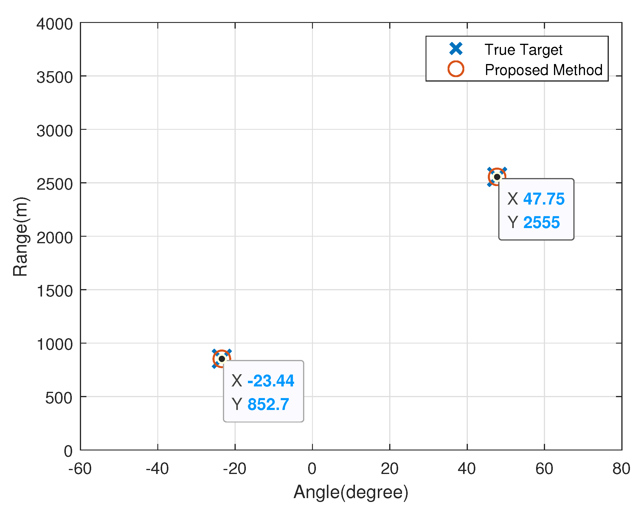
5.1. Two-Dimensional Point Cloud of Target Parameters

In the first simulation, Figure 2 shows the location of the estimated targets in the spatial domain, where SNR $=20$ dB and $T=50$. The X-axis and Y-axis denote DOA and range, respectively. It can be seen from Figure 2 that the target can be explicitly distinguished, which demonstrates the effectiveness of the proposed method.

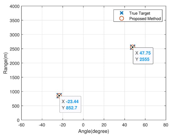
Figure 2. Two-dimensional point cloud image of estimated targets.

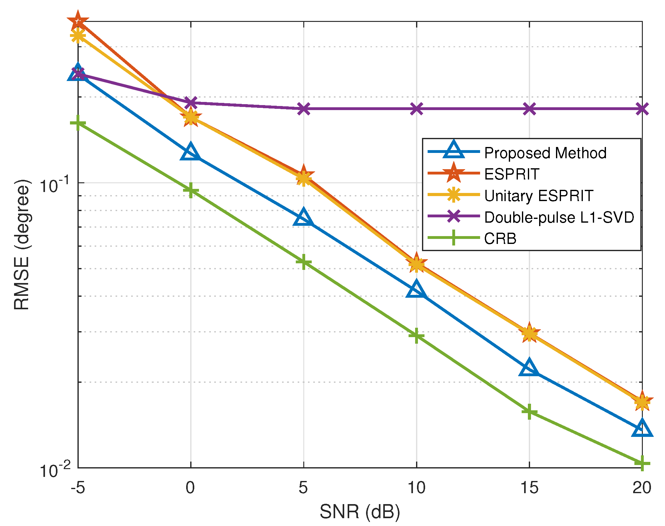
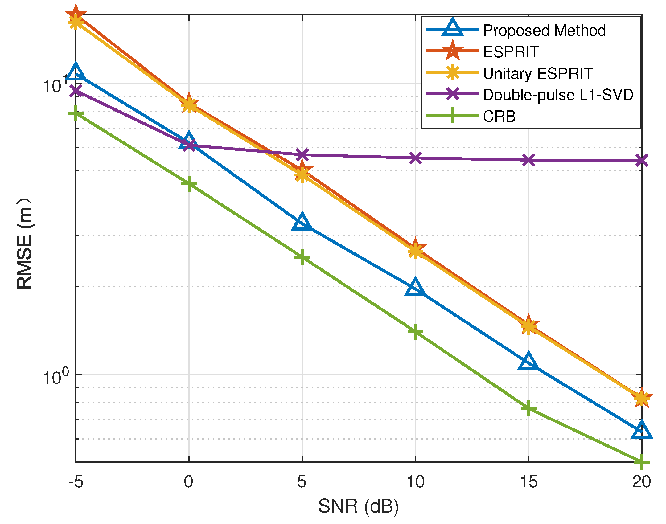
5.2. RMSE versus SNR

In this part, we compare the proposed method and three typical methods including ESPRIT [27], unitary-ESPRIT [28], and double-pulse $l_1$-SVD [42]. Moreover, CRB is provided as the performance evaluation metric. The root mean square error (RMSE) is introduced and can be defined by

$$RMS{E}_{\theta }=\frac{1}{K}\sum _{k=1}^K\sqrt{\frac{1}{V}\sum _{v=1}^V{({\theta }_{v,k}-{\theta }_k)}^2}$$

(64)

$$RMS{E}_r=\frac{1}{K}\sum _{k=1}^K\sqrt{\frac{1}{V}\sum _{v=1}^V{(r_{v,k}-r_k)}^2}$$

(65)

where ${\theta }_{v,k}$ and $r_{v,k}$ denote the estimates of ${\theta }_k$ and $r_k$ in the v-th Monte Carlo trial, respectively. $V=100$ is the number of Monte Carlo trials.

In Figure 3 and Figure 4, we provide the RMSE results of DOA and range with different SNR conditions, where $T=50$. In the double-pulse $l_1$-SVD method, we set the DOA grid interval within $[-{90}^{\circ },{90}^{\circ }]$ to ${0.5}^{\circ }$, and the range grid interval within $[0,4000]$ m to $10m$. Figure 3 and Figure 4 depict the RMSE results of the DOA and range estimates under different SNR conditions, respectively. Specifically, the double-pulse $l_1$-SVD method is limited by its lower error bound because it fails to solve the off-grid gap problem, and the RMSE results does not improve with the increase in SNR when the error lower bound is reached. Additionally, we can conclude that the proposed method outperforms the methods in [27,28,42]. The fundamental reason for this is that the proposed method not only overcomes the problem that the performance of subspace method will significantly deteriorate in the case of low SNR or scarce snapshots, but also manages to solve the off-grid gap caused by the discrete grids.

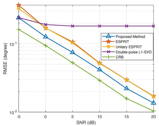
Figure 3. RMSE of DOA estimation versus SNR.

Figure 4. RMSE of range estimation versus SNR.

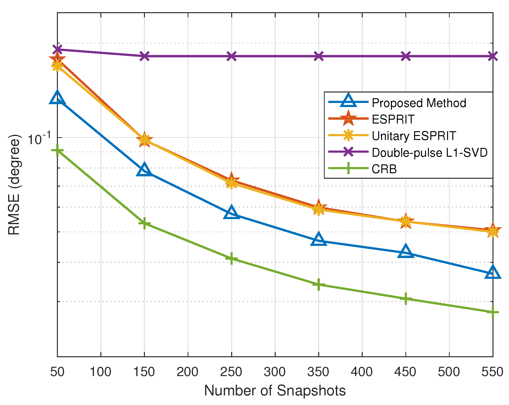
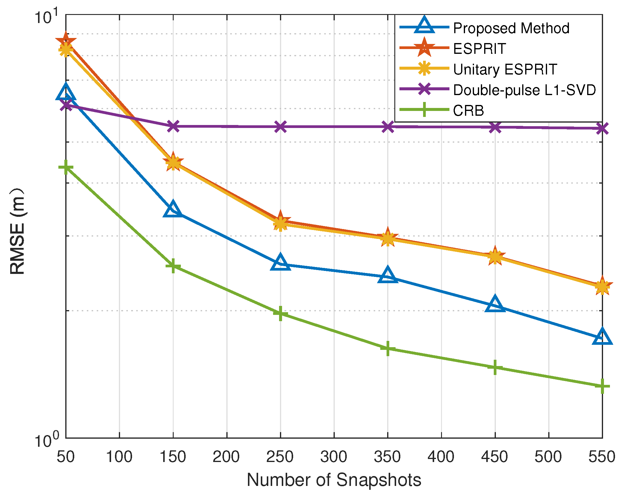
5.3. RMSE versus Snapshots

In this simulation, we evaluate the DOA and range estimation performance versus snapshots to further verify the effectiveness of the proposed method. The snapshots vary from 50 to 550 with an SNR = 0 dB. Similarly, we introduced CRB to measure the performance of the proposed method. According to Figure 5 and Figure 6, the RMSE results of all methods improve with the increase in snapshots. In particular, the proposed method is superior to the other methods in DOA and range estimation accuracy with different numbers of snapshots. Among all the methods, since the double-pulse $l_1$-SVD method suffers from the off-grid gap, its RMSE results no longer decrease with the increase in snapshots, when the snapshots reach the lower bound of the error.

Figure 5. RMSE of DOA estimation versus snapshots.

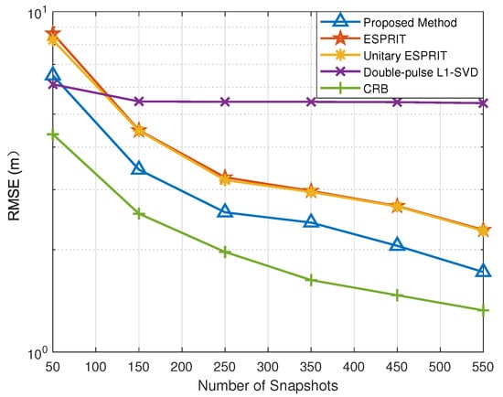
Figure 6. RMSE of range estimation versus snapshots.

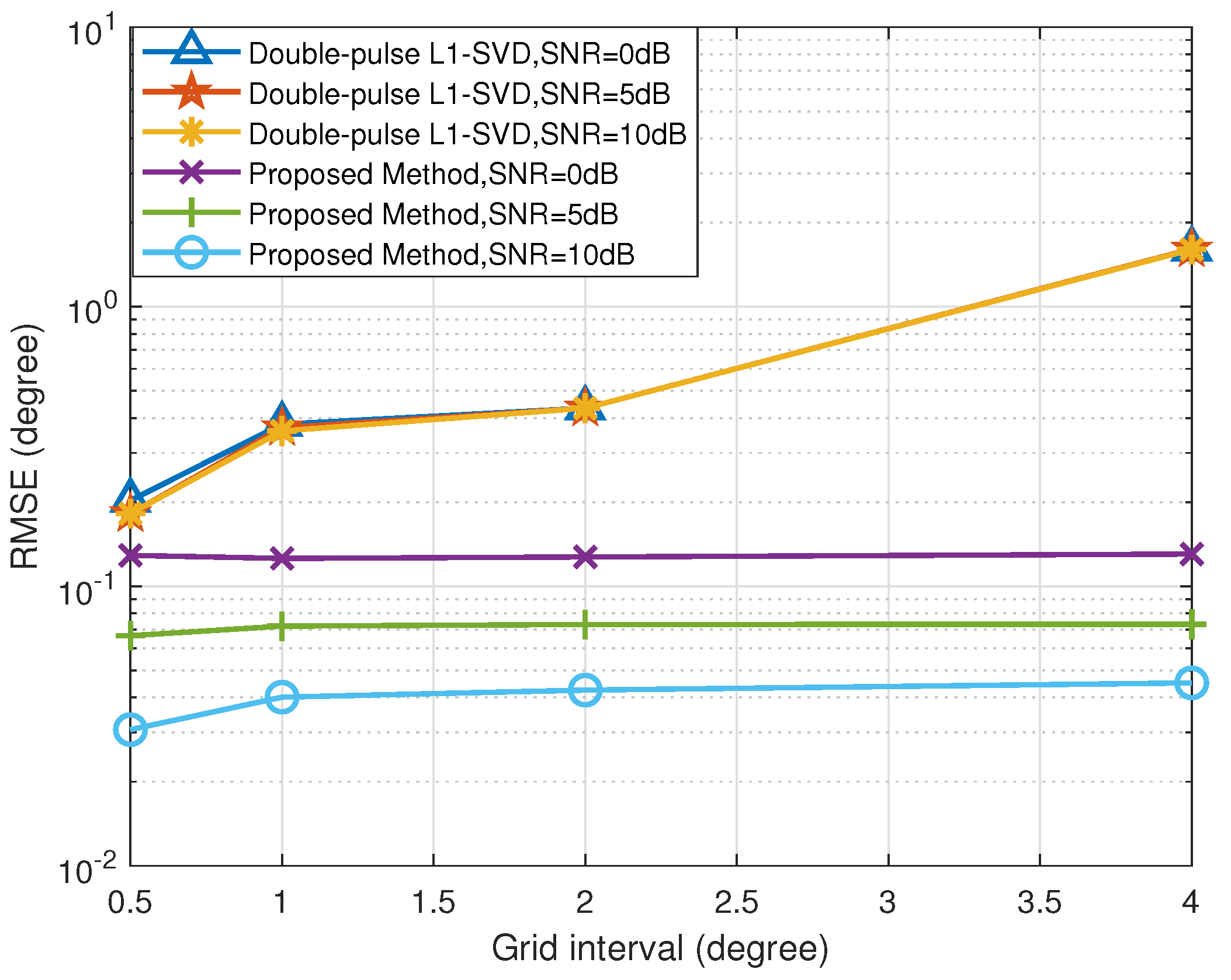
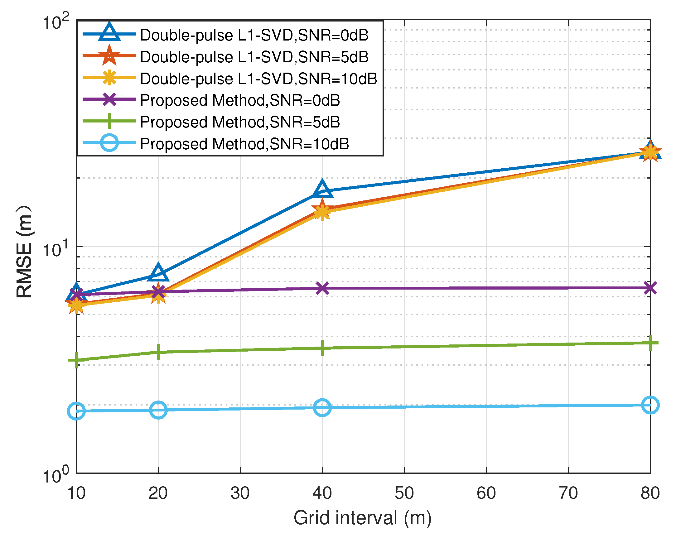
5.4. RMSE versus Grid Interval

In order to further verify the robustness of the proposed method with respect to the off-grid gap, we give the RMSE results of the proposed method with different off-grid gaps. The double-pulse $l_1$-SVD method, which also belongs to the family of SSR methods, is selected to compare with the proposed method. Figure 7 and Figure 8 depict the RMSE results of the DOA and range estimates with different grid intervals, respectively, where $T=$ 50. Under different grid intervals, the proposed method can obtain better estimation performance than the double-pulse $l_1$-SVD method, which benefits from the fact that the proposed method solve the problem of the off-grid gap. In addition, according to Figure 7 and Figure 8, the RMSE results of the proposed method improve with the increase in SNR. Since the double-pulse $l_1$-SVD method suffers from the off-grid gap, its RMSE results no longer decrease with the increase in SNR. The reason for this is that the double-pulse $l_1$-SVD method fails to accurately construct the real observation model with a coarse sampling grid and encounters the degradation of estimation performance.

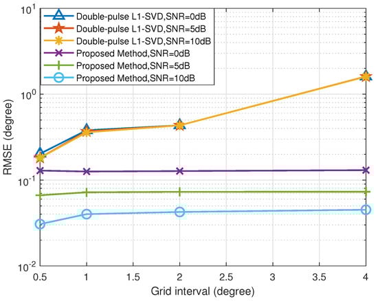
Figure 7. RMSE of DOA estimation versus grid interval.

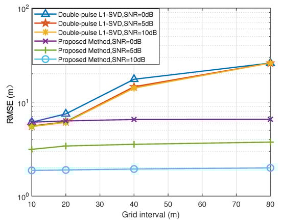
Figure 8. RMSE of range estimation versus grid interval.

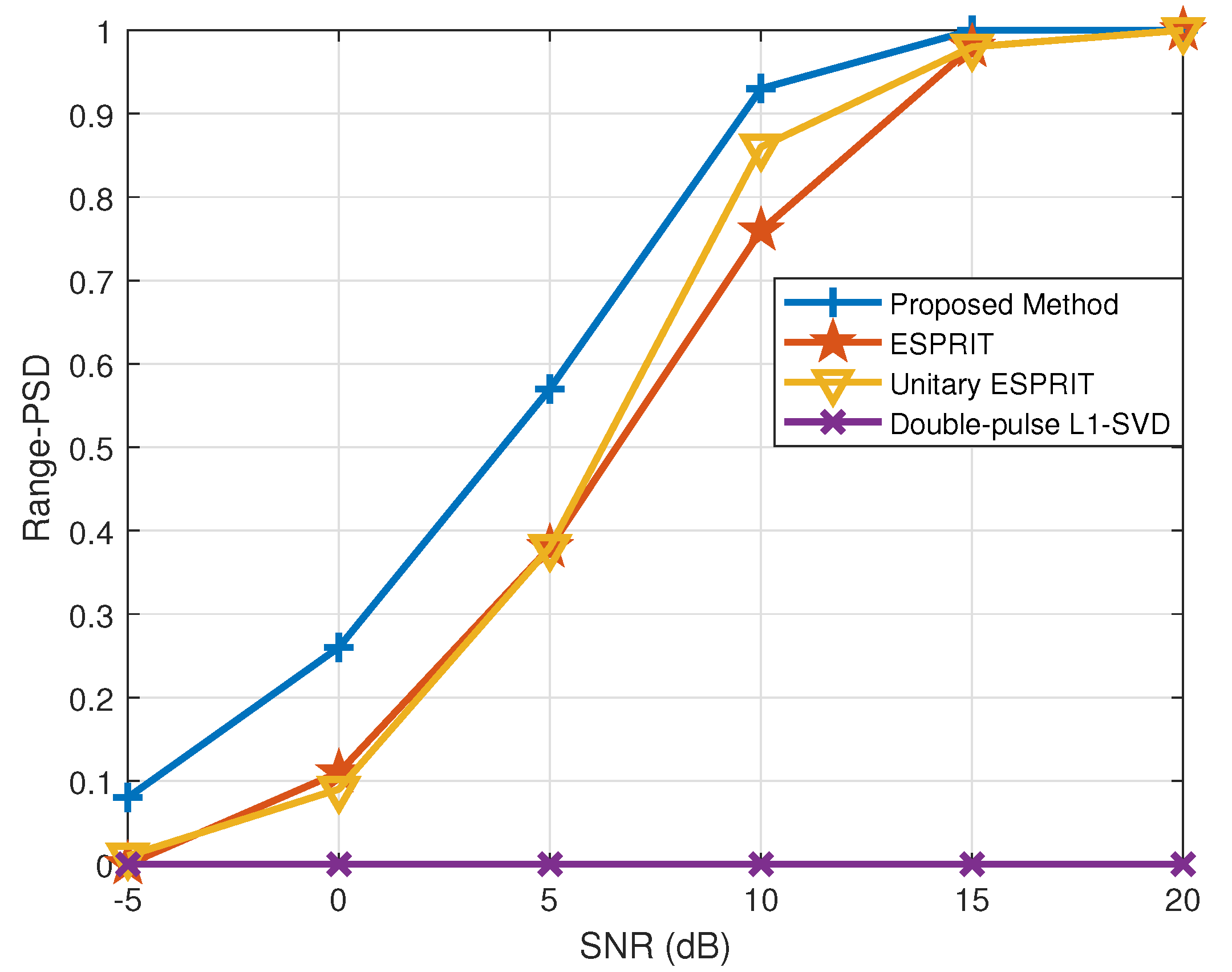
5.5. PSD versus SNR

The probability of successful detection (PSD) is adopted to measure the performance of the proposed method, which can be defined by

$$PSD=\frac{H}{V}\times 100$$

(66)

where H denotes the number of successful estimation.

In this subsection, the DOA estimation is considered to be successful when $\left|{\theta }_{v,k}-{\theta }_k\right|$$\le {0.15}^{\circ }$ while the range estimation is successful when $\left|r_{v,k}-r_k\right|\le 4m$. Figure 9 and Figure 10 depict the PSD of DOA and range estimation in different SNR conditions, respectively, where $T=50$. It is clearly shown that the proposed method outperforms the other methods at different SNR as the proposed method can first reach 100% PSD with the increase in the SNR. Additionally, the double-pulse $l_1$-SVD method fails to accurately construct the real observation model with a coarse sampling grid, so the error lower bound of this method does not meet the criteria for successful detection.

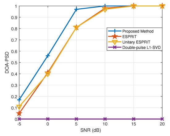
Figure 9. PSD of DOA estimation versus SNR.

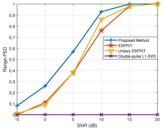
Figure 10. PSD of range estimation versus SNR.

6. Conclusions

In this paper, an effective off-grid SBL method is proposed, which enables the calculation the DOA and range estimates. Firstly, the angle-dependent component is split by reconstructing the received data and allows the immediate extraction of rough DOA estimates with the root SBL algorithm, which, subsequently, are utilized to obtain the paired rough range estimates. Furthermore, a discrete grid is constructed by the rough DOA and range estimates, and the 2D-SBL model is proposed to optimize the rough estimates of DOA and range. Finally, the EM algorithm is utilized to update the grid points iteratively to further eliminate the errors caused by the off-grid model. Moreover, the proposed method belongs to the SSR method, which overcomes the shortcomings of the subspace method in that the performance is significantly attenuated in the case of a low SNR or scarce snapshots. Massive simulation results have verified that the proposed method can carry out DOA and range estimation accurately. In future work, we will further improve the performance of the proposed method and implement it through a hardware system to apply it to actual scenarios.

References

- Smith, C.M.; Feder, H.; Leonard, J.J. Multiple target tracking with navigation uncertainty. In Proceedings of the 37th IEEE Conference on Decision and Contro, Tampa, FL, USA, 18 December 1998; pp. 760–761. [Google Scholar]
- Sammartino, P.F.; Baker, C.J.; Rangaswamy, M. Moving target localization with multistatic radar systems. In Proceedings of the 2008 IEEE Radar Conference, Rome, Italy, 26–30 May 2008; pp. 1–6. [Google Scholar]
- Krim, H.; Viberg, M. Two decades of array signal processing research: The parametric approach. IEEE Signal Process. Mag. 1996, 13, 67–94. [Google Scholar] [CrossRef]
- Wan, L.; Sun, Y.; Sun, L.; Ning, Z. Deep Learning Based Autonomous Vehicle Super Resolution DOA Estimation for Safety Driving. IEEE Trans. Intell. Transp. Syst. 2020, in press. [Google Scholar] [CrossRef]
- Perna, S.; Soldovieri, F.; Amin, M. Editorial for Special Issue “Radar Imaging in Challenging Scenarios from Smart and Flexible Platforms”. Remote Sens. 2020, 12, 1272. [Google Scholar] [CrossRef] [Green Version]
- Premachandra, C.; Murakami, M.; Gohara, R. Improving landmark detection accuracy for self-localization through baseboard recognition. Int. J. Mach. Learn Cyber. 2017, 8, 1815–1826. [Google Scholar] [CrossRef]
- Cavanini, L.; Benetazzo, F.; Freddi, A. SLAM-based autonomous wheelchair navigation system for AAL scenarios. In Proceedings of the 2014 IEEE/ASME 10th International Conference on Mechatronic and Embedded Systems and Applications (MESA), Senigallia, Italy, 10–12 September 2014; pp. 1–5. [Google Scholar]
- Wang, X.; Yang, L.T.; Meng, D. Multi-UAV Cooperative Localization for Marine Targets Based on Weighted Subspace Fitting in SAGIN Environment. IEEE Internet Things J. 2021, in press. [Google Scholar]
- Hu, Z.; Zeng, Z.; Wang, K. Design and Analysis of a UWB MIMO Radar System with Miniaturized Vivaldi Antenna for Through-Wall Imaging. Remote Sens. 2019, 11, 1867. [Google Scholar] [CrossRef] [Green Version]
- Shi, J.; Wen, F.; Liu, T. Nested MIMO Radar: Coarrays, Tensor Modeling and Angle Estimation. IEEE Trans. Aerosp. Electron. Syst. 2021, 57, 573–585. [Google Scholar]
- Wan, L.; Liu, K.; Liang, Y.; Zhu, T. DOA and Polarization Estimation for Non-Circular Signals in 3-D Millimeter Wave Polarized Massive MIMO Systems. IEEE Trans. Wirel. Commun. 2021, 20, 3152–3167. [Google Scholar] [CrossRef]
- Wang, X.; Wan, L.; Huang, M. Polarization Channel Estimation for Circular and Non-Circular Signals in Massive MIMO Systems. IEEE J. Sel. Top. Signal Process. 2019, 13, 1001–1016. [Google Scholar] [CrossRef]
- Wang, X.; Wan, L.; Huang, M. Low-Complexity Channel Estimation for Circular and Noncircular Signals in Virtual MIMO Vehicle Communication Systems. IEEE Trans. Veh. Technol. 2020, 69, 3916–3928. [Google Scholar] [CrossRef]
- Antonik, P.; Wicks, M.C.; Griffiths, H.D. Frequency diverse array radars. In Proceedings of the 2006 IEEE Conference on Radar, Verona, NY, USA, 24–27 April 2006; pp. 215–217. [Google Scholar]
- Wang, W.Q. Frequency Diverse Array Antenna: New Opportunities. IEEE Antennas Propag. Mag. 2015, 57, 145–152. [Google Scholar] [CrossRef]
- Wang, W.Q. Overview of frequency diverse array in radar and navigation applications. IET Radar Sonar Navig. 2016, 10, 1001–1012. [Google Scholar] [CrossRef]
- Wang, C.; Xu, J.; Liao, G. A Range Ambiguity Resolution Approach for High-Resolution and Wide-Swath SAR Imaging Using Frequency Diverse Array. IEEE J. Sel. Top. Signal Process. 2017, 2, 336–346. [Google Scholar] [CrossRef]
- Wang, W.Q.; Shao, H. Range-Angle Localization of Targets by A Double-Pulse Frequency Diverse Array Radar. IEEE J. Sel. Top. Signal Process. 2014, 8, 106–114. [Google Scholar] [CrossRef]
- Wang, W.Q. Subarray-based frequency diverse array radar for target range-angle estimation. IEEE Trans. Aerosp. Electron. Syst. 2014, 50, 3057–3067. [Google Scholar] [CrossRef]
- Liu, Y.; Hang, R.; Wang, L. The Random Frequency Diverse Array: A New Antenna Structure for Uncoupled Direction-Range Indication in Active Sensing. IEEE J. Sel. Top. Signal Process. 2017, 11, 295–308. [Google Scholar] [CrossRef]
- Khan, W.; Qureshi, I.M.; Saeed, S. The Random Frequency Diverse Array: A New Antenna Structure for Uncoupled Direction-Range Indication in Active Sensing. IEEE Antennas Wirel. Propag. Lett. 2015, 14, 499–502. [Google Scholar] [CrossRef]
- Zhang, J.J.; Papandreousuppappola, A. MIMO Radar with Frequency Diversity. In Proceedings of the 2009 International Waveform Diversity and Design Conference, Kissimmee, FL, USA, 8–13 February 2009; pp. 208–212. [Google Scholar]
- Sammartino, P.F.; Baker, C.J.; Griffiths, H.D. Frequency Diverse MIMO Techniques for Radar. IEEE Trans. Aerosp. Electron. Syst. 2013, 49, 201–222. [Google Scholar] [CrossRef]
- Xu, J.; Liao, G.; Zhu, S. Joint Range and Angle Estimation Using MIMO Radar With Frequency Diverse Array. IEEE Trans. Signal Process. 2015, 63, 3396–3410. [Google Scholar] [CrossRef]
- Sammartino, P.F.; Baker, C.J.; Griffiths, H.D. Range-angle dependent waveform. In Proceedings of the 2010 IEEE Radar Conference, Arlington, VA, USA, 10–14 May 2010; pp. 511–515. [Google Scholar]
- Liu, F.; Wang, X.; Huang, H. Joint Angle and Range Estimation for Bistatic FDA-MIMO Radar via Real-valued Subspace Decomposition. Signal Process. 2021, 185, 108065. [Google Scholar] [CrossRef]
- Li, B.; Bai, W.; Zheng, G. Successive ESPRIT algorithm for joint DOA-range-polarization estimation with polarization sensitive FDA-MIMO radar. IEEE Access. 2018, 6, 36376–36382. [Google Scholar] [CrossRef]
- Liu, F.; Wang, X.; Huang, M. A Novel Unitary ESPRIT Algorithm for Monostatic FDA-MIMO Radar. Sensors 2020, 20, 827. [Google Scholar] [CrossRef] [Green Version]
- Xiong, J.; Wang, W.Q.; Gao, K. FDA-MIMO Radar Range-Angle Estimation: CRLB, MSE and Resolution Analysis. IEEE Trans. Aerosp. Electron. Syst. 2018, 54, 284–294. [Google Scholar] [CrossRef]
- Wan, L.; Kong, X.; Xia, F. Joint Range-Doppler-Angle Estimation for Intelligent Tracking of Moving Aerial Targets. IEEE Internet Things J. 2018, 5, 1625–1636. [Google Scholar] [CrossRef]
- Chen, P.; Chen, Z.; Zhang, X.; Liu, L. SBL-Based Direction Finding Method with Imperfect Array. Electronics 2018, 7, 426. [Google Scholar] [CrossRef] [Green Version]
- Zheng, R.; Xu, X.; Ye, Z.F. Sparse Bayesian learning for off-grid DOA estimation with Gaussian mixture priors when both circular and non-circular sources coexist. Signal Process. 2019, 161, 124–135. [Google Scholar] [CrossRef]
- Malioutov, D.; Cetin, M.; Willsky, A.S. A sparse signal reconstruction perspective for source localization with sensor arrays. IEEE Trans. Signal Process. 2005, 8, 3010–3022. [Google Scholar] [CrossRef] [Green Version]
- Yin, J.; Chen, T. Direction-of-Arrival Estimation Using a Sparse Representation of Array Covariance Vectors. IEEE Trans. Signal Process. 2011, 59, 4489–4493. [Google Scholar] [CrossRef]
- Liu, S.; Tang, L.; Bai, Y.; Zhang, X. A Sparse Bayesian Learning-Based DOA Estimation Method With the Kalman Filter in MIMO Radar. Electronics 2020, 9, 347. [Google Scholar] [CrossRef] [Green Version]
- Ling, Y.; Gao, H.; Zhou, S.; Yang, L.; Ren, F. Robust Sparse Bayesian Learning-Based Off-Grid DOA Estimation Method for Vehicle Localization. Sensors 2020, 20, 302. [Google Scholar] [CrossRef] [Green Version]
- Cao, Z.; Zhou, L.; Dai, J. Sparse Bayesian Approach for DOD and DOA Estimation with Bistatic MIMO Radar. IEEE Access. 2019, 7, 155335–155346. [Google Scholar] [CrossRef]
- Yang, Z.; Xie, L.; Zhang, C. Off-grid Direction of Arrival Estimation Using Sparse Bayesian Inference. IEEE Trans. Signal Process. 2013, 61, 38–43. [Google Scholar] [CrossRef] [Green Version]
- Dai, J.; Bao, X.; Xu, W. Root Sparse Bayesian Learning for Off-Grid DOA Estimation. IEEE Signal Process. Lett. 2017, 24, 46–50. [Google Scholar] [CrossRef] [Green Version]
- Wen, F.; Huang, D.; Wang, K.; Zhang, L. DOA estimation for monostatic MIMO radar using enhanced sparse Bayesian learning. J. Eng. 2018, 5, 268–273. [Google Scholar] [CrossRef]
- Chen, P.; Cao, Z.; Chen, Z.; Wang, X. Off-Grid DOA Estimation Using Sparse Bayesian Learning in MIMO Radar With Unknown Mutual Coupling. IEEE Trans. Signal Process. 2019, 67, 208–220. [Google Scholar] [CrossRef] [Green Version]
- Liu, Q.; Wang, X.; Wan, L. An Accurate Sparse Recovery Algorithm for Range-Angle Localization of Targets via Double-Pulse FDA-MIMO Radar. Wirel. Commun. Mob. Comput. 2020, 3, 1–12. [Google Scholar]
- Cui, C.; Jian, X.; Gui, R. Search-Free DOD, DOA and Range Estimation for Bistatic FDA-MIMO Radar. IEEE Access. 2018, 6, 15431–15445. [Google Scholar] [CrossRef]
- Wang, H.; Wan, L.; Dong, M. Assistant Vehicle Localization Based on Three Collaborative Base Stations via SBL-Based Robust DOA Estimation. IEEE Internet Things J. 2019, 6, 5766–5777. [Google Scholar] [CrossRef]
- Ji, S.; Xue, Y.; Carin, L. Bayesian Compressive Sensing. IEEE Trans. Signal Process. 2008, 56, 2346–2356. [Google Scholar] [CrossRef]
- Zhang, X.; Xu, D. Angle estimation in bistatic MIMO radar using improved reduced dimension Capon algorithm. J. Syst. Eng. Electron. 2013, 24, 84–89. [Google Scholar] [CrossRef]
Publisher’s Note: MDPI stays neutral with regard to jurisdictional claims in published maps and institutional affiliations. |
© 2021 by the authors. Licensee MDPI, Basel, Switzerland. This article is an open access article distributed under the terms and conditions of the Creative Commons Attribution (CC BY) license (https://creativecommons.org/licenses/by/4.0/).