Recognition of the Typical Distress in Concrete Pavement Based on GPR and 1D-CNN

Abstract

Ground-penetrating radar (GPR) signal recognition depends much on manual feature extraction. However, the complexity of radar detection signals leads to conventional intelligent algorithms lacking sufficient flexibility in concrete pavement detection. Focused on these problems, we proposed an adaptive one-dimensional convolution neural network (1D-CNN) algorithm for interpreting GPR data. Firstly, the training dataset and testing dataset were constructed from the detection signals on pavement samples of different types of distress; secondly, the raw signals are were directly inputted into the 1D-CNN model, and the raw signal features of the radar wave are extracted using the adaptive deep learning network; finally, the output used the Soft-Max classifier to provide the classification result of the concrete pavement distress. Through simulation experiments and actual field testing, the results show that the proposed method has high accuracy and excellent generalization performance compared to the conventional method. It also has practical applications.

1. Introduction

Roads are the city’s most important transport facilities. As roads are used, distress appears on the road pavement. Pavement often contains voids, disengaging, no compactness, and other distress. The emergence and development of pavement distress are hidden, which may cause significant damage (Figure 1). We detected and evaluated pavement distress to analyze the distress causes. It minimizes the damage done by the distress to protect the security infrastructure and maintain the normal operations of the infrastructure [1,2,3].

Ground-penetrating radar (GPR) is a high-resolution non-destructive testing method applied to the pavement. It can effectively detect distress in the pavement. G.Leimbach and H.Lowy first proposed to make use of GPR to detect the distribution characteristics of underground bodies. Then, they acquired a patent for GPR in 1910 [4]. Geophysical Survey Systems Inc. (GSSI) invented the first commercial GPR-SIR radar in the 1970s, and in 1995, it produced the first GPR system for highway quality detection. The effective application of GPR depends not only on the implementation of a hardware system, but also on signal processing and data interpretation technology. The GPR reflection signal identification technology can improve GPR from extensive use in detecting distress in the concrete pavement [5,6,7,8].

Methods for recognizing distress in concrete include processing the GPR signal, feature selection, and signal recognition. The quality of the recognition model is directly related to the recognition effect. So, establishing a high accuracy recognition model is the key to solving the problem of pavement distress recognition [9,10,11]. The most common method in the literature is the Hough Transform method [12]. Despite pavement distress recognition achieved by some methods, on top of that, problems of false alarms have not been fully resolved [13]. Many scholars have researched the scientific issues to focus on the problem. Davis et al. proposed the use of a back-propagation neural network (B.P.) and radial basis function network (RBF) using the feature extraction radar waves to identify internal defects in the concrete. However, this method has an intense subjectivity, and the accuracy of the evaluation is not high [14,15]. For solving the recognition accuracy problem of the conventional neural network, Xie et al. used the support vector machine (SVM) to classify the type of pavement distress based on GPR detection. The process entails the non-linear function transformation of the map feature vectors of radar signal maps into high dimensional feature space, and the optimal hyperplane is constructed in high dimensional space for sample classification. However, the classification accuracy is greatly affected by the feature vector selected, which limits the ability to make widespread use of this method [16,17]. Pouria et al. used the AdaBoost machine learning algorithm based on the GPR histogram of oriented gradients (HOG) feature to identify the steel in the bridge deck. This method is an integration of several classifiers for the classification of the GPR image. However, the method still needs to select radar image features [18,19]. In spite of the above method having a specific effect, the manual extraction of certain features is generally useful only for specific data. The mentioned methods cannot directly extract the feature from the raw GPR signal. The conventional machine learning (ML) methods are challenging to promote the development of detection technology.

Recently, deep learning theory has gradually become the main development direction for machine learning [20,21]. Deep learning network architecture automatically extracts the features of the sample layer by layer, which is independent of the artificial feature extraction and expert knowledge. It has been widely applied in natural language processing, pattern recognition, visual computer tasks, and machine fault diagnosis [22,23,24]. As an essential branch of deep learning, the convolution neural network (CNN) has mainly been used in the sequence feature extraction of two-dimensional (2D) and three-dimensional (3D) images in recent years. Some scholars have introduced CNN into the GPR field [25,26]. Chae et al. focused on classifying B-scans of GPR cylinders according to their depth, size, material, and the dielectric constant of the underlying medium using convolutional neural networks [27,28]. Kien et al. presented an automated rebar localization and detection algorithm based on the integration of conventional image processing techniques and deep convolutional neural networks [29,30]. Namguy et al. used CNN for the underground object detection of urban road pavement based on a large amount of GPR B-scan image libraries [31,32]. These methods used the CNN algorithm for GPR 2D image recognition. The self-learning ability of CNN has not been fully utilized. The radar signal is a 1D typical time-series signal, and its data correlates with every time point. If the 1D raw radar signal is transformed into a two-dimensional image form, and the original sequence space correlation is destroyed, then the original information in the raw data is lost [33,34,35,36].

In summary, the pavement distress detection methods are divided into two types: the combination of artificial design features and traditional ML classification algorithms or CNN based on candidate regions for recognition. Artificial design features can not fully detect road distress, traditional ML classification algorithm has difficulty dealing with a complex road environment, and CNN algorithm based on candidate areas can not realize real-time detection. It is necessary to study an effective automatic recognition algorithm for GPR data interpretation.

At present, 1D-CNN research on the classification of the GPR signal field is still in the exploratory stage. The primary advantage of 1D-CNN is that a real-time and low-cost hardware implementation is feasible due to the compact and straightforward configuration of 1D CNNs that perform only 1D convolutions [37]. It brings a challenge to explore 1D-CNN in the GPR data interpretation field. In this paper, the raw radar signal is directly set as an input, and the 1D-CNN method is established for GPR signal recognition. The method is independent of feature extraction and maximizes the implementation of the self-learning function of CNN to generate the intelligence recognition model of the GPR signal. The proposed 1D-CNN-based GPR signal cognition approach was developed and verified using experimental simulation data for a benchmark pavement GPR detection problem and useful pavement detection data. The significance of this work can be summarized as follows:

• Unlike the conventional machine learning method based on GPR signal cognition available in the literature, the proposed method directly operates on the raw GPR signal without the need for manual feature extraction. The high-level features of the GPR signal are automatically extracted through the convolutional operation layer of 1D-CNN.
• Conventional machine learning methods applied to GPR signals use manual features that are limited by the specific data set. The proposed CNN-based method uses the optimal features learned by the 1D-CNNs to maximize classification accuracy. It is the critical property that significantly improves classification performance.
• Furthermore, we showed the cognition classification results have high accuracy in one simulation experiment in benchmark pavement GPR detection and one practical pavement detection experiment.

This paper is organized as follows: The authors discussed previous studies on object detection with GPR data in Section 1. The novel approach to distress detection/localization in concrete pavement GPR field data based on 1D-CNN is proposed and introduced in Section 2. A detailed description of the implementation of the proposed method and performance study is provided in Section 3 and Section 4. The main conclusions are listed in Section 5.

2. Theory and Methodology

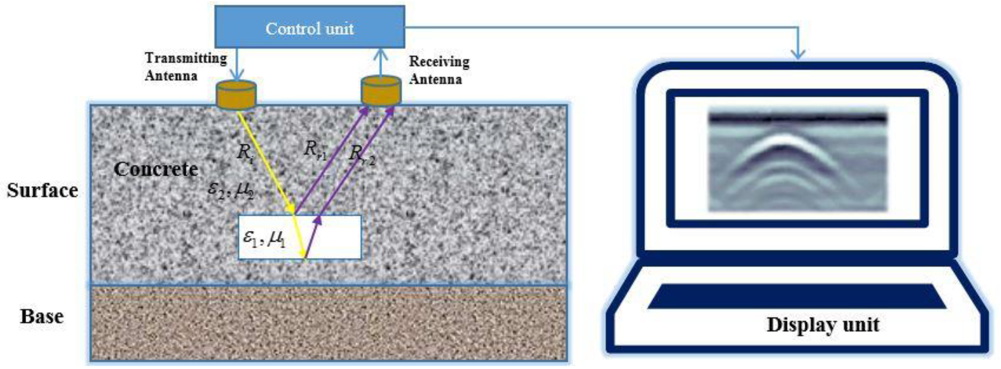
2.1. GPR Detection Concrete Distress Theory

GPR transmit antennas send high-frequency electromagnetic waves into the concrete. As the electromagnetic waves propagate in the medium, the reflection of the electromagnetic waves occurs when the electromagnetic waves are faced with electromagnetic differences in the target. According to the transmission waveform signal, the reflected waves collected by the receiving antenna detect subsurface anomalies, wave amplitude, two-way travel time, and other parameters (Figure 1). The application of GPR has evolved from geophysical field applications to civil engineering applications.

In the time domain, the composite wavelet can be expressed as the convolution of the GPR incident wave $R_i\left(t\right)$ with the reflectivity series $r\left(t\right)$ and noise $n\left(t\right)$:

$$R_r\left(t\right)=R_i\left(t\right)\ast r\left(t\right)+n(t)$$

(1)

Based on the assumption of the plane wave, the effective reflection coefficients of the top and bottom interfaces are as follows:

$$r_1=\frac{\sqrt{{\epsilon }_2}-\sqrt{{\epsilon }_1}}{\sqrt{{\epsilon }_2}+\sqrt{{\epsilon }_1}}$$

(2)

$$r_2=\left(1-r_1^2\right)\frac{\sqrt{{\epsilon }_1}-\sqrt{{\epsilon }_2}}{\sqrt{{\epsilon }_2}+\sqrt{{\epsilon }_1}}$$

(3)

where ε₁ and ε₂ are the relative dielectric constants of the concrete and void regions, respectively.

The transmission coefficient of the void layer is defined as:

$$T=e^{-j2\omega b/v}$$

(4)

where $\omega$ is the composite wavelet frequency, $b$ is the attenuation constant, and $v$ is the velocity in the medium.

Based on Figure 1, the composite wavelet consists of two reflections from the top and bottom interfaces. The wavelet can be defined as:

$$R_r=R_{r1}+R_{r2}$$

(5)

Based on Equations (1)–(5), the amplitude spectrum of $R_r\left(t\right)$ in the frequency domain can be expressed as the following:

$$A_r\left(\omega \right)=A_i\left(\omega \right)H\left(\omega \right)=A_i\left(\omega \right)\left(r_1+r_2{T}^2\right)$$

(6)

where $A_r\left(\omega \right)$ and $A_i\left(\omega \right)$ are the amplitude spectrums of $R_r\left(t\right)$ and $R_i\left(t\right)$ respectively.

The data interpretation of GPR generally includes two aspects (data processing and image interpretation):

• Data processing includes preprocessing (marking and station correction, etc.) and post-processing. Its primary purpose is to suppress interference and highlight sound signals under the condition of ensuring resolution to make the degree of reflection wave as clear as possible. It can extract various valuable parameters (such as electromagnetic wave velocity, waveform, etc.).
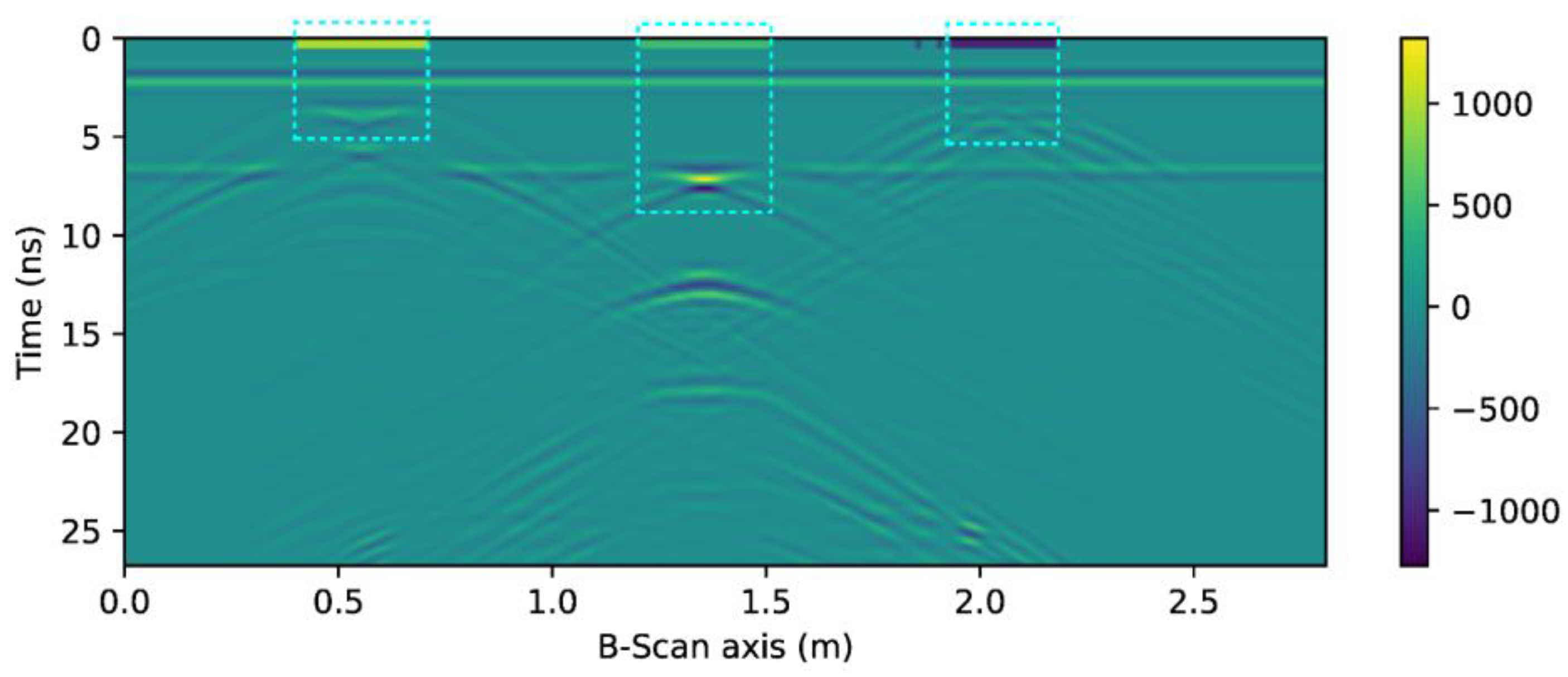
• The purpose of image interpretation is to analyze the processed time profile and interpret the anomalies. In the process of interpretation, the reflection signals are interpreted qualitatively and quantitatively according to the appearance features of the image, such as reflection intensity and phase features, and combining with drilling data and other supporting data.

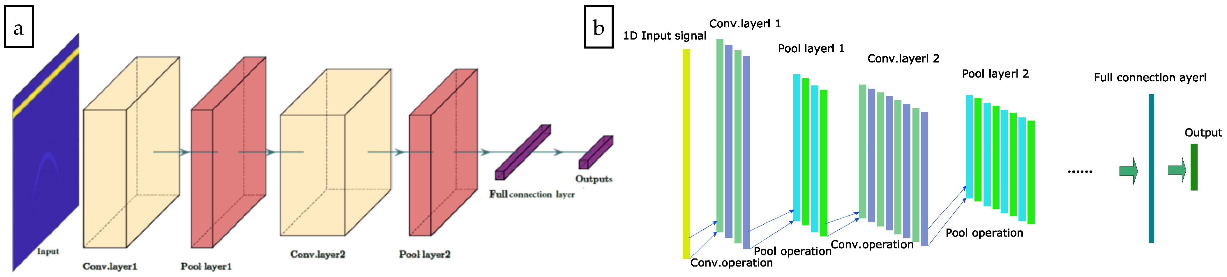
2.2. One-Dimensional Convolution Neural Network

CNN is sensitive to local information, and the global information is obtained from higher-level neurons and the fusion of different layers of local information. The CNN structure constitutes an alternation of the convolutional layer and the pooling layer (Figure 2a).

However, the convolution kernel and feature image are two-dimensional in a conventional CNN. The GPR signal is a typical one-dimensional signal, and a conventional CNN cannot directly implement the classification of the GPR signal. So, we proposed the a 1D-CNN to classify the GPR signal. The input signal is one-dimensional in 1D-CNN. The vectors of the convolution kernel and feature image within the network are also one-dimensional. The structure is shown in Figure 2b.

In a 1D-CNN, the assumption of $l$ the layer is the convolutional layer. The expression of the 1D convolutional layer is as follows:

$$x_j^l=f\left({\displaystyle \sum _{i=1}^M{x}_i^{l-1}\ast k_{ij}^l+b_j^l}\right)$$

(7)

where $x_j^l$ is the $j$st feature mapping in $l$ the layer, $f$ is the activate function, $M$ is the number of input feature maps, $\ast$ is the convolution operation, $k_{ij}^l$ is the trainable convolutional kernel, and $b_j^l$ is the bias.

The activation function $f$ meant to improve the convergence rate and reduce over-fitting benefits. The Rectified Linear Unit (ReLU) is one of the essential activation functions. The ReLU activation function is as follows:

$$\mathrm{Re}LU\left(x\right)=\max \left(0,x\right)$$

(8)

The assumption that $l+1$ the layer is the pooling layer, and then $l+1$ the layer is shown as:

$$s_j^l=f\left(down\left(x_i^l\right)+b_j^l\right)$$

where $down(·)$ is the down-sampling function that is the sum of all elements of the vector $n\times 1$, as down-sampling only affects the overlap region. Thus, the result is the size of the original $1/n$.

The pooling layer of the assumption is $l+1$ layer as a feature vector, and the input vector $s_i^{l+1}$ is a single layer perceptron. Therefore, the output vector can be expressed as:

$$y_i^{{}^{l+1}}=f\left(W_{}^{{}^{l+1}}{s}_i^{{}^{l+1}}+b_{}^{{}^{l+1}}\right)$$

(9)

where $W^{l+1}$ are the weights and $b^{l+1}$ is the bias.

CNN training is based on the back-propagation (B.P.) principle, which minimizes the mean square error during the convolution kernel training and bias training. The L-BFGS algorithm avoids directly solving the Hessian matrix. In place of approximating the Hessian matrix, the partial gradient operator and model correction is saved to solve the pseudo-Hessian matrix [38]. It avoids occupying much memory space and computation time for the Hessian matrix requirement.

The GPR detection signal has a close correlation with the partial sample, and the long-distance between the samples has a weak correlation. So, the 1D-CNN can easily extract and learn the features of the raw radar signal. During the construction of the 1D-CNN, the raw GPR signal corresponding to the sample label data is first used for training the 1D-CNN. In the 1D-CNN, the feature extraction model is constituted alternately of convolution layers and pool layers. Then, the classification vector is used for training the Soft-Max classification model. Finally, the trained network model feature extraction combines with the Soft-Max classifier model to build one integral 1D-CNN. The network model training process is shown in Figure 3.

The training process is divided into two phases in the GPR 1D-CNN. Firstly, during the training of the 1D-CNN, the neural network parameters are initialized, and the neural network parameters are trained using the BP algorithm. The network error or iteration times reach the set requirements, and the classification vector can be obtained. Secondly, the classification vectors of the neural network are used as inputs to train the Soft-Max classifier model, and the iteration computation does not stop until the iteration times reach the set maximum. Finally, network training accuracy needs to be tested. If the solution meets the accuracy requirements, the network model is saved. Otherwise, the convolution kernel size of the pool of nuclear factors needs to be reset.

3. GPR Numerical Simulation Model Experiment

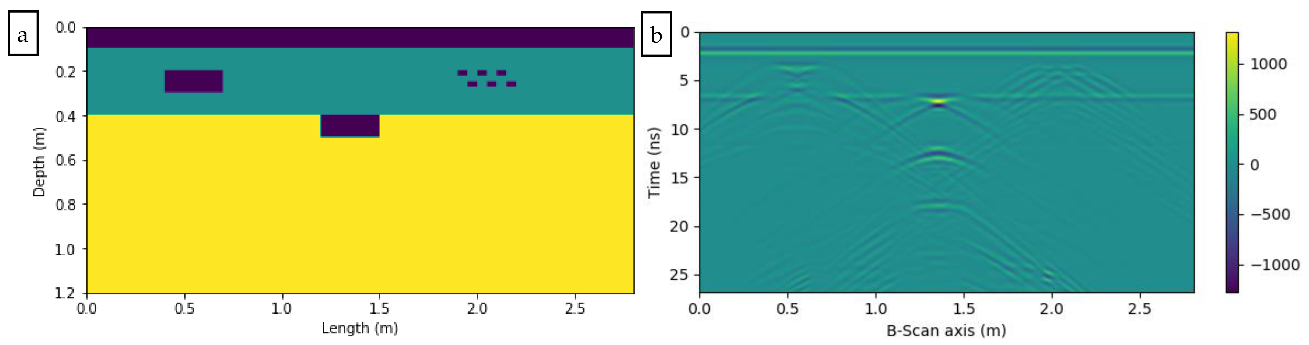
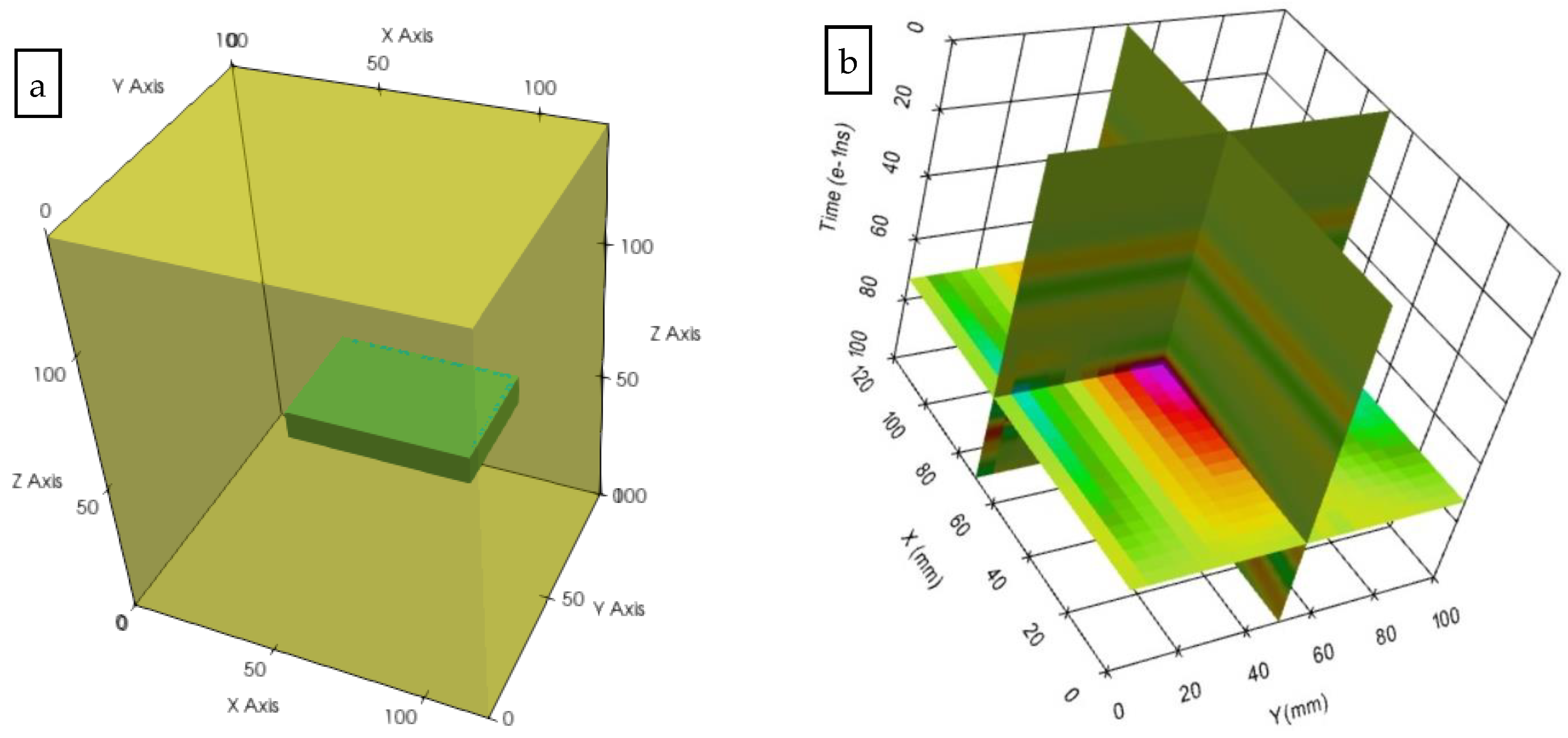
3.1. Pavement GPR Detection Benchmark Simulation

A simulation model was created to evaluate the contribution of 1D-CNN based on the Matlab 2016 platform (The MathWorks, Natick, MA, USA). The established pavement model is shown in Figure 4a. The dimensions were 2.8 × 1.2 m². The model consisted of three layers: 0.1 meter thick air (ε = 1.0, σ = 0 ms/m), 0.3 meter thick surface layer (ε = 6, σ = 1 ms/m), and 0.8 meter thick base (ε = 16, σ = 5 ms/m). Three distresses (void, disengaging, and no compactness) were embedded in the model. The sizes were 0.3 × 0.1 m². The corresponding depths were 0.1 m, 0.3 m, and 0.1 m.

During the simulation of the GPR with the finite difference time domain (FDTD), the hardware platform utilized was Intel Core i5-6200 central processing unit dual-core 2.3 GHz, random access memory 8.0 GB. The computational grid size was 0.005 m, and the length of the time window was 40 ns. The sample number was 512. The central frequency of the transceiver antenna was set to 900 MHz, the transceiver antenna distance is 0.01 m, and the work mode was self-excitation and self-receiving. The scanner result of the simulation was shown in Figure 4b.

There are 281 traces of GPR signals in the experimental test results; 90 traces were in the anomaly; 30 traces were located at each hidden distress. In total, 200 trace signals were randomly selected as a training dataset, with the remaining portion set as a testing dataset. Based on the establishment of the data sets, the 1D-CNN was used to study the recognition of pavement distress (A. Normal; B. Void; C. Disengaging; D. No compactness).

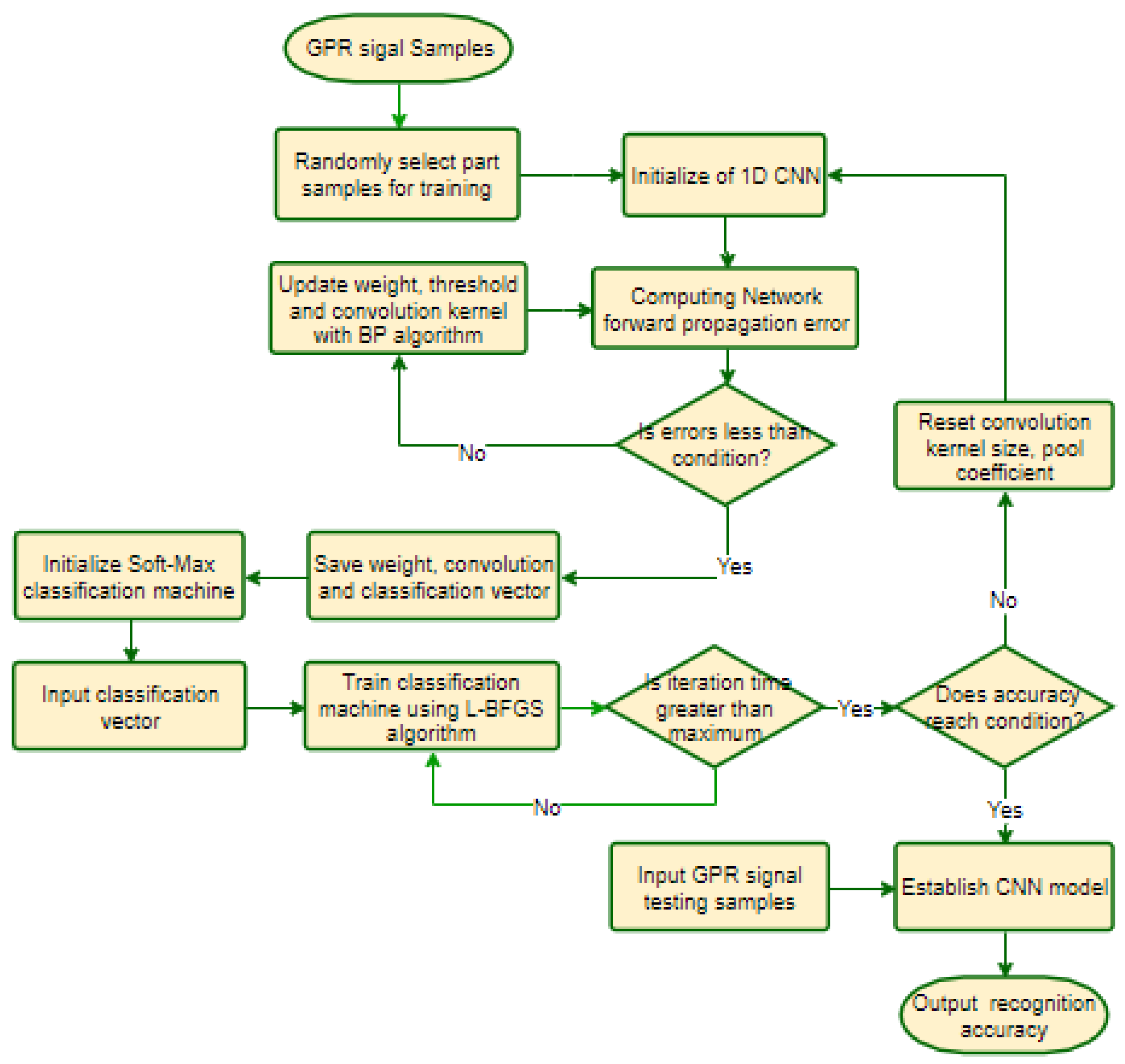
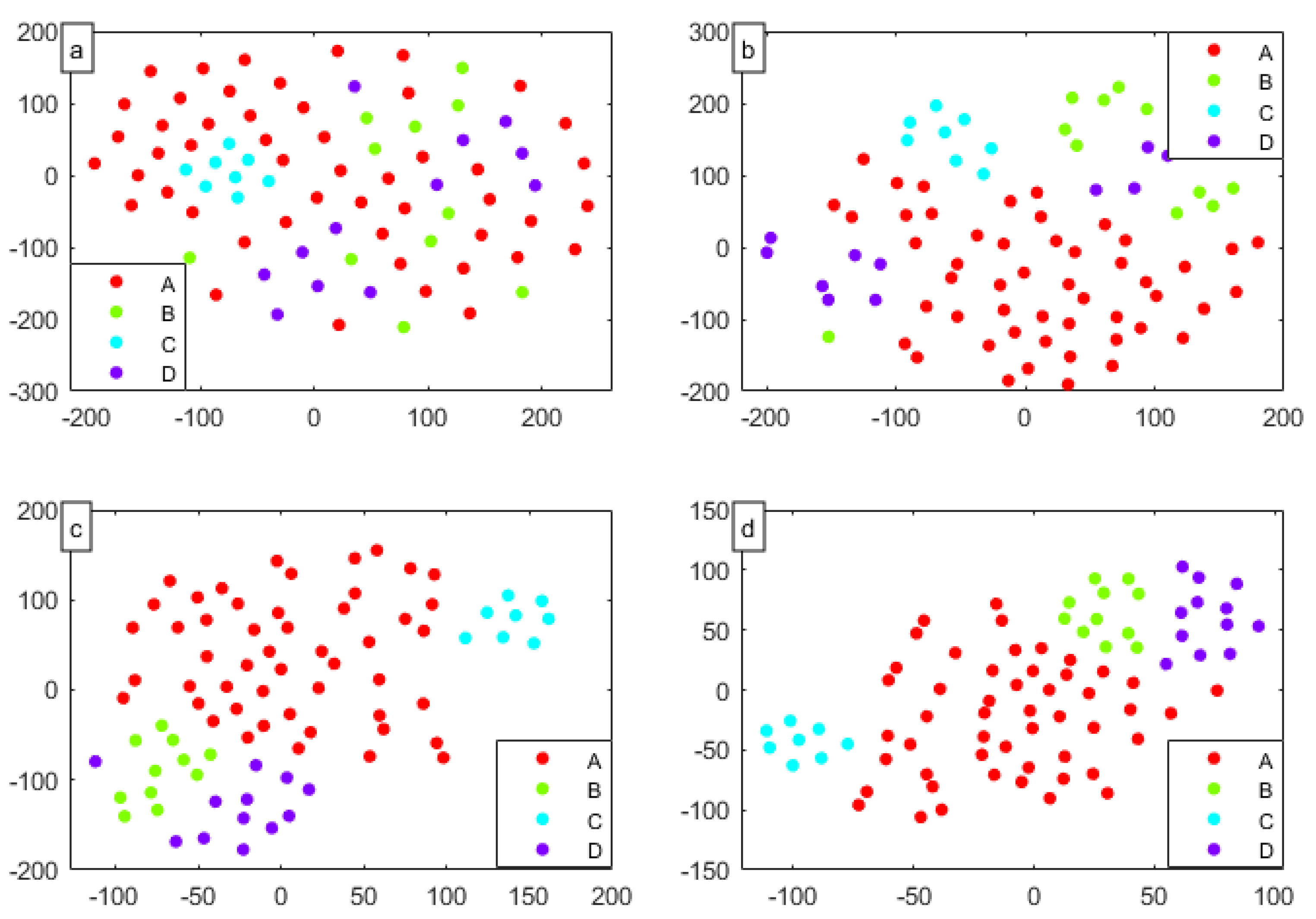
3.2. Design and Hyperparameter Optimization of 1D-CNN

In the experiment, the 1D-CNN is composed of two convolutional neural layers, two pool layers, and the perception of one full connection layer. There are four categories (Normal, Hole, Disengaging, and No compactness) regarding the health status of the pavement. During the 1D-CNN training process, the inputs are the raw 1D GPR signal data while the corresponding outputs are $\left(1,0,0,0\right)$, $\left(0,1,0,0\right)$,$\left(0,0,1,0\right)$ and $\left(0,0,0,1\right)$ respectively. The construction of the 1D-CNN model and the selection of appropriate model parameters are the premises for ensuring high accuracy. Furthermore, the solution efficiency was also considered. It is necessary to optimize the structure of 1D-CNN and the training parameters involved as much as possible. We focused on the design of the 1D-CNN. The effect experiments of the parameters were involved in determining the size of the convolutional kernel and the training parameters.

3.2.1. Effect Analysis of the Size of Convolution Layer Neurons

Most of the time, we increased the number of convolutional neural layers or the number of convolution neurons to improve solution accuracy. As the GPR signal is a typical 1D radar wave model, the sample dimension was low, and the number of training samples was limited. The number of convolution layers was fixed at two convolution layers to avoid over-fitting of the CNN. We considered the influence of different configurations and training parameters of the 1D-CNN for the training and test samples classification accuracy, while the training time was considered a reference evaluation index. Due to the error between the actual output and the expected output, the network structure needs training to solve the final classification results. The 1D-CNN can directly input the raw GPR data to train the network model without preprocessing the signals, such as dimension reduction, filtering, etc.

When setting the number of neurons in the hidden layer, the number of neurons in one fore layer was not more than one-half the neurons in one back layer. In the study, eight different types of neuron configurations were tested. The experimental results are shown in

Table 1. The effect of different neuron configurations on the recognition rate.

Neuron Configuration	Recognition Accuracy (%)		Training Time (s)
	Train	Test
16, 8	93.00	90.12	11.75
32, 8	94.50	91.19	18.06
32, 16	96.00	93.83	20.78
64, 16	96.50	92.59	31.92
64, 32	96.50	92.59	35.57
128, 32	97.00	96.30	59.64
128, 64	97.00	96.30	66.38
256, 64	97.00	95.06	113.30

.

According to Table 1, the model training samples can enhance the ability to identify categories by increasing the number of convolution kernels. However, it increases the training time-cost. When using the neuron configuration (128, 32), the recognition rate of the training sample is highest, and the time consumed is lower than that of the last two configuration styles; in the case where the arrangement of neurons uses the (128, 32) configuration, the testing recognition rate is optimal, and the time spent is about half of the neurons using the (256, 64) configuration. Considering both the recognition rate of the testing set and the training time indicators, we selected the neurons of the convolutional model (128, 32) configuration.

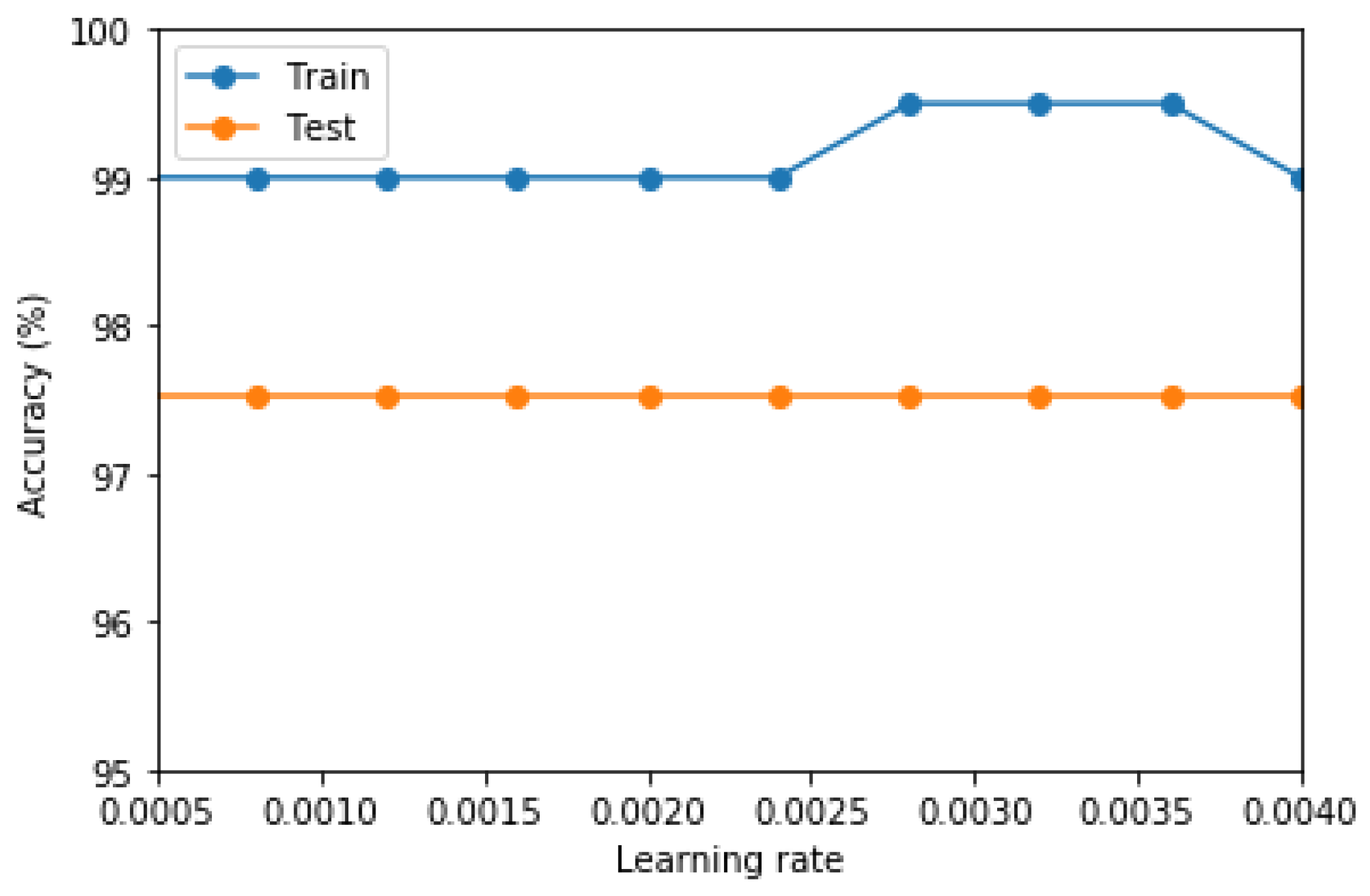
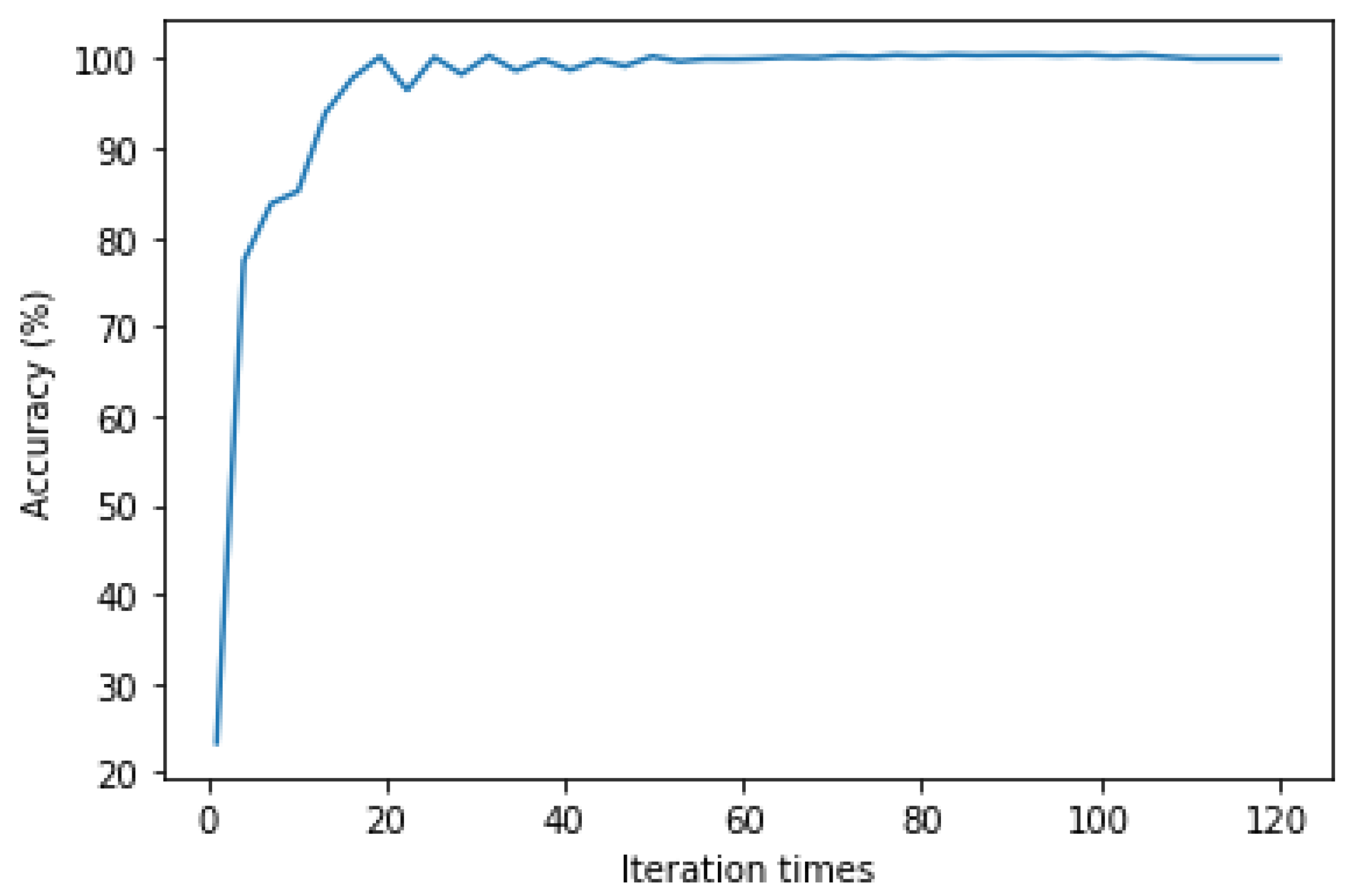
3.2.2. Effect Analysis of the Learning Rate and Training Iterations

The learning rate of CNN is an essential parameter in the training process, which directly affects the stability and convergence rate of CNN. If the learning rate is too large, the numerical results appear to diverge, and the neural network cannot be trained appropriately; if the learning rate is too low, the neural network training speed slows down, and the training time increases exponentially. The training iteration times were tested in the research, and the influence of the learning rate was studied. The recognition accuracy of concrete pavement distress is shown in Figure 5, changing with the training iteration times.

According to Figure 5, the learning rate of the training parameters is within the range between 0.0005 and 0.004. There is a maximum value in the range between 0.0028 and 0.0036. It shows the excellent classification performance of the network, and the learning rate affects the CNN recognition accuracy to a certain extent. As the trained neural network has high accuracy, the learning rate does not significantly affect the recognition accuracy in the range.

Under the appropriate learning rate, the increasing number of iterations can reduce network errors and obtain higher accuracy. In Figure 6, the learning rate is 0.003. With the increasing number of iterations, the network computation error gradually decreases, as shown in Figure 6.

In Figure 6, with the increase in the iterative number, the recognition accuracy gradually increases. When the iteration number reaches 50, the change in the accuracy of the network stabilizes. Then, the efficiency is not significantly improved as the iterations increase. The iterative number was set to 50 times in the 1D-CNN.

3.3. Performance Analysis and Comparison of the 1D-CNN

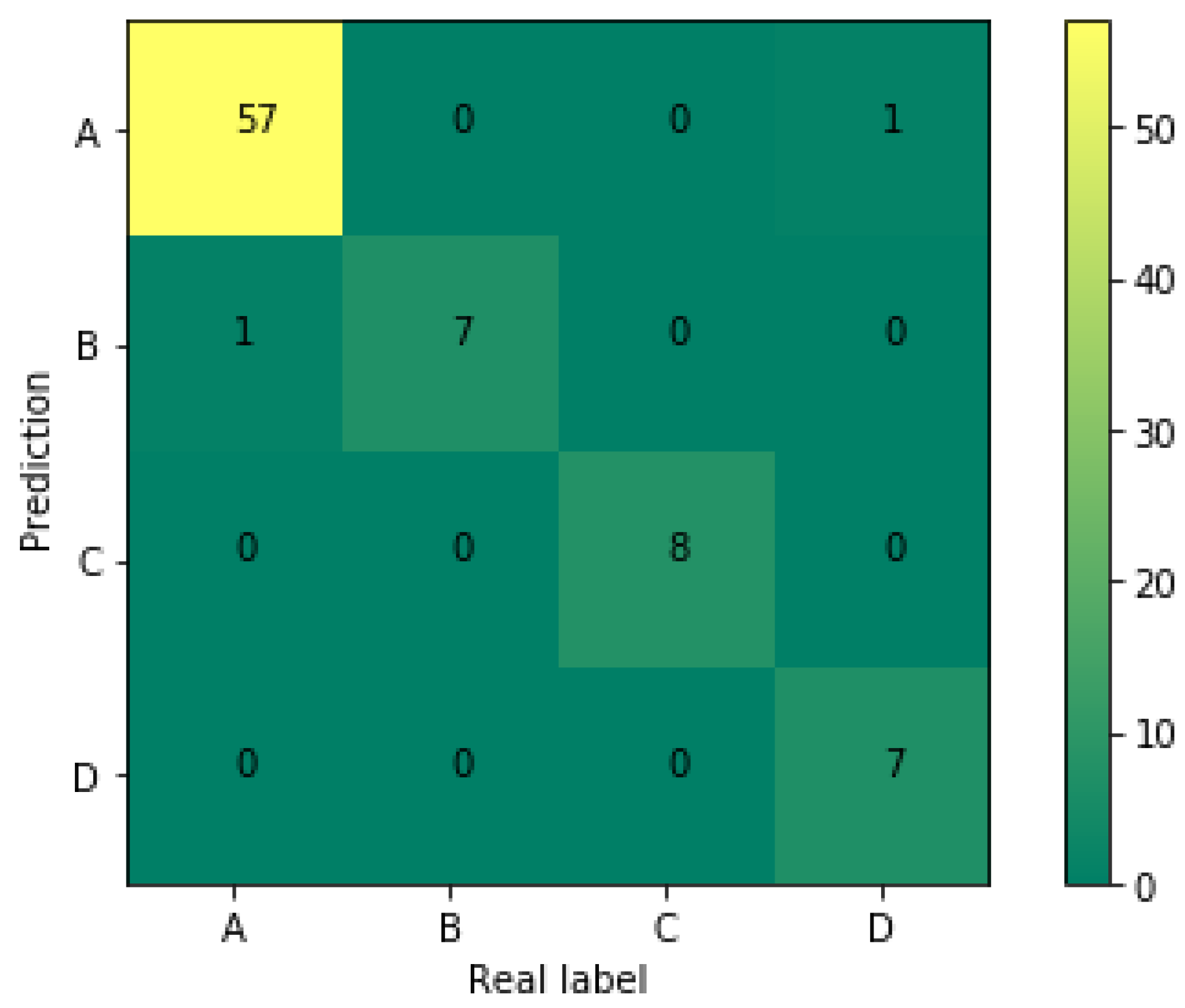
3.3.1. D-CNN Performance Analysis

Based on the structure and training parameters of the 1D-CNN, the GPR 1D-CNN was applied to recognize each category in the testing set. After 50 iterations, the classification accuracy of the testing set reached 97.5%. It shows that the algorithm has a high ability to recognize pavement distress in GPR detection. To more clearly demonstrate each category’s recognition in the test, the confusion matrix was introduced in the performance analysis of the 1D-CNN. The confusion matrix is shown in Figure 7.

According to Figure 7, there is only one case of no compactness distress that is misrecognized, and the recognition accuracies of the two categories even reached 100%. This shows that the proposed method is accurate in recognizing concrete pavement distress based on GPR detection.

To further study the convolutional layer and the pooling layer on the effect of the deep learning feature, the data was reduced to two-dimensional data, and visualization of the non-linear dimensionality reduction algorithm was obtained. Herein, the extracted two-dimensional elements in different levels of the output vector feature were visualized using t-Distributed Stochastic Neighbor Embedding (t-SNE). The results are shown in Figure 8.

Figure 8a shows the analysis results of the raw input. Due to the redundancy of the raw radar signal, it was difficult to distinguish between each category individually. After the first convolution learning layer, the sample distribution of input significantly improved from Figure 8b, and most categories were gathered in their respective regions. However, part of the sample still did not have clustering. In Figure 8c, through the second convolutional learning layer, each category sample shows more aggregate than the first convolutional layer, with only a small amount of the samples having been misclassified. In Figure 8d, each category sample gathers in their respective regions, and all of the samples were classified correctly.

Then, the trained 1D-CNN was used to recognize pavement distress in the entire cross-section. The recognition result of the distresses displays in lines. In Figure 9, the three-line region represents the recognition result of the distress (Yellow line: Void; Green line: Disengaging; Blue line: No compactness).

According to the defection region in Figure 9, there are three lines on the synthetic B-Scan. Compared with the location of distresses in Figure 4a, three categories of concrete defects are correctly recognized with 1D-CNN in Figure 9. The proposed algorithm can accurately recognize the distribution of three different defects in the pavement.

3.3.2. Performance Comparison of Different Methods

In GPR signal recognition, the 1D-CNNModel is not only simple but has high recognition accuracy. To further test the network performance, the 1D-CNN performance was compared with the conventional method. First, the eight kinds of statistical features extracted from the data set were set as the input vector. There are five machine learning methods— to be tested, including BP neural network, support vector machine (SVM), extreme learning machine (ELM), and Adaboost classifier. The five methods identified the established GPR simulated data sets. The corresponding recognition results are shown in

Table 2. Performance comparison of the different methods.

ML Algorithm	Recognition Accuracy (%)		Training Time (s)
	Train	Test
BP	67.00	61.72	3.8
SVM	86.50	82.50	19.61
ELM	69.50	64.20	0.0012
Adaboost	96.00	90.12	1.34
1D-CNN	97.00	96.30	66.38

.

In Table 2, there are significant differences among the classification results of the five machine learning classification algorithms. 1D-CNN presents the highest recognition accuracy and can accurately identify the different kinds of concrete pavement distress. 1D-CNN does not require feature extraction radar signals in advance and only has a longer training time than other algorithms, but this does not affect the practical application of the method. Compared to the conventional machine learning algorithm, it has significant advantages.

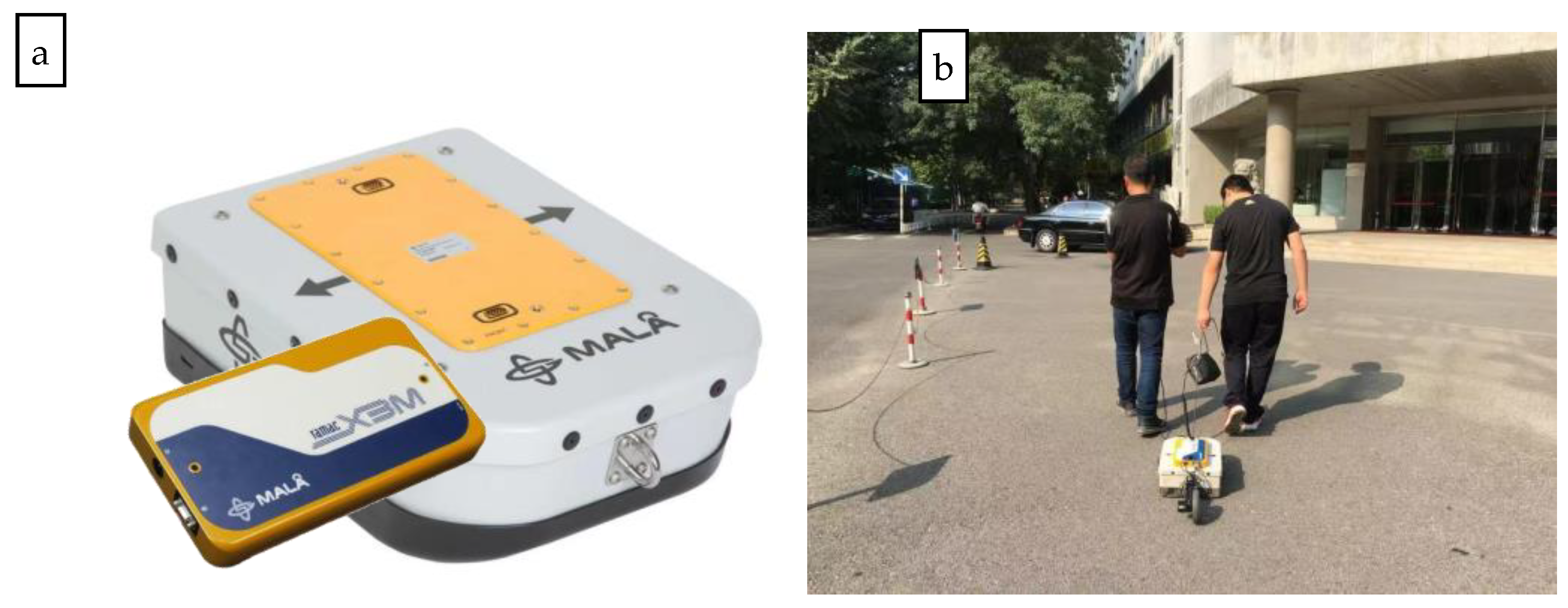
4. Engineering Application

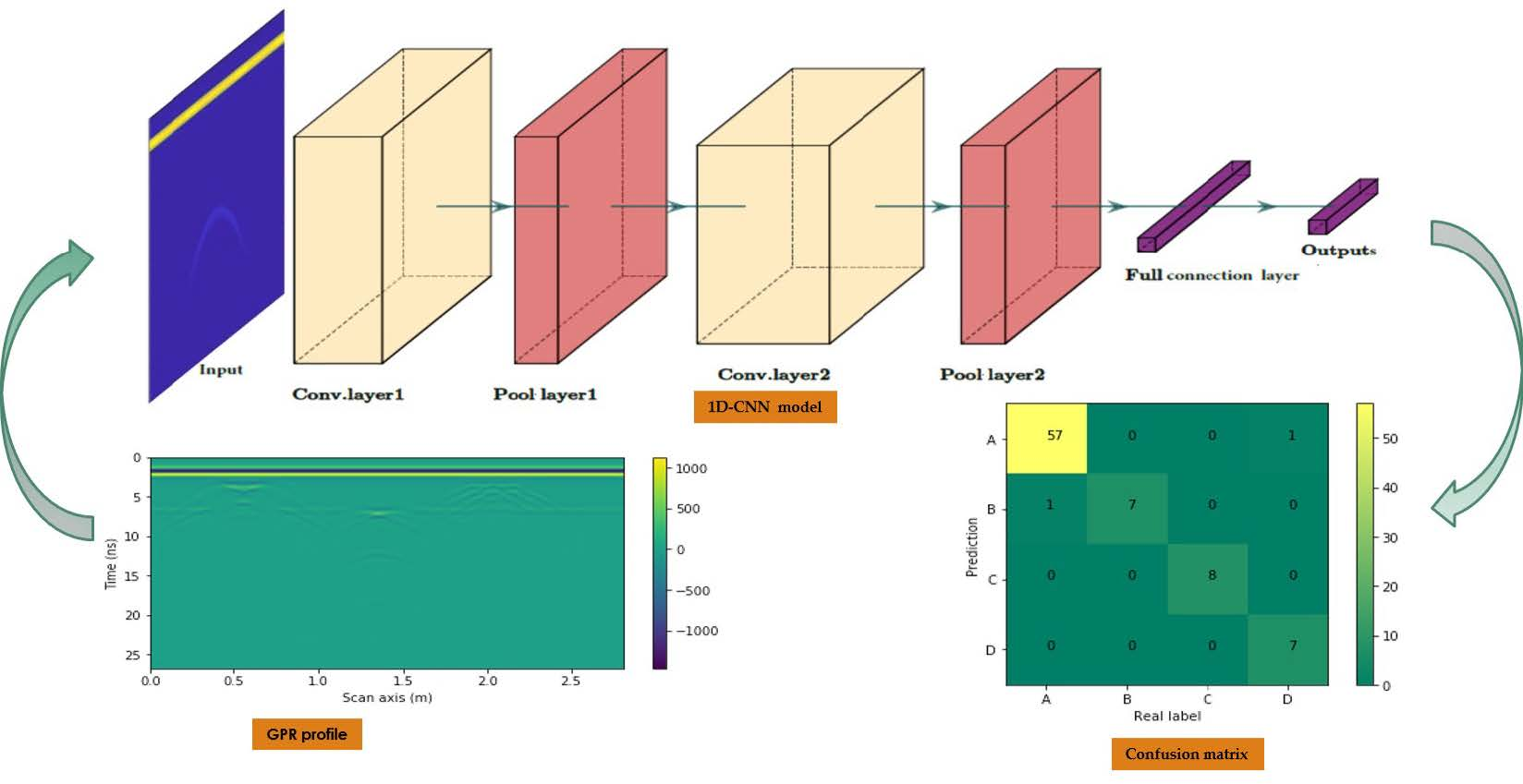
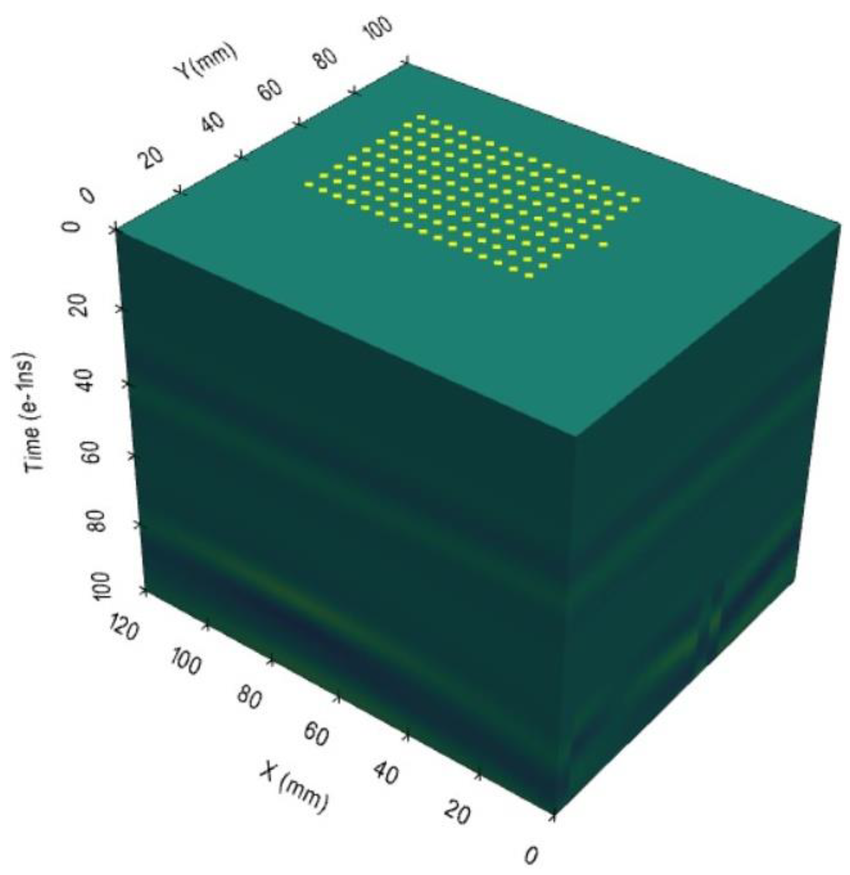
4.1. Distress Recognization in Pavement Engineering

We implemented the application of the established 1D-CNN and investigated the highways in the Nanjing City of China with GPR. The detection device used was a Mala GPR X3M controller and had a shielded antenna with a 500 MHz central frequency (Figure 10a). Figure 10b shows GPR real-life validation test site. One length of the detection section studied was 10.0 m. The acquisition space interval was 0.02 m, and the cross-section contained 500 trace records, with each trace having 512 sampling points.

Figure 11a shows the survey records of the GPR. According to the established 1D-CNN based on Section 3, the convolution layer is used for feature extraction of GPR signals, and the Soft-Max classifier is used to obtain categories. The inputs are the raw 1D GPR signal data while the corresponding outputs are $\left(1,0,0,0\right)$ or $\left(0,1,0,0\right)$ respectively. In total, 200 trace data were randomly selected from the 500 trace data as the training set for 1D-CNN. In the process of training, the size of each batch is 50, and the learning rate is set to 0.006. The hardware platform utilized was Intel Core i5-6200 central processing unit dual-core 2.3 GHz, random access memory 8.0 GB. 1D-CNN was trained for 100 epochs. Then, the trained 1D-CNN was used to recognize pavement distress in the entire cross-section. In Figure 10b, the yellow line region represents the recognition result of the distresses.

According to the distress region in Figure 11b, the GPR diagram displays discontinuity in the surface layer and is significantly different from the other sections. The concrete distress region of the recognition matches the actual no compactness concrete region very well. One spot in the distress region was exposed for validation (Figure 12). The evidence shows distress existed in the region. Thus, 1D-CNN has an excellent ability to recognize distress in pavement engineering using GPR detection.

4.2. Interpretation of 3D-GPR Detection

The 3D-GPR uses three-dimensional array antennas to collect three-dimensional data, which has higher spatial resolution and measurement accuracy for road distress. 3D-GPR detected the road in the area took the cavity in the pavement as the distress body in this case. The cavity was a 60 mm × 40 mm × 10 mm rectangular block. The horizontal projection is located at the position of the simulation area (55 mm, 70 mm), and the depth of its center point was 60mm from the surface. The position and shape are shown in Figure 13a. A 20-channel 3-D GPR was simulated, and a 1.5 GHz Ricker wavelet was used in the case.

The hardware platform utilized was Intel Core i7-10710U central processing unit six-core 1.61 GHz, random access memory 16.0 GB. In the same way, the 3D data of 3D-GPR detection was obtained through the forward simulation of the FDTD method. The 3D data body contained 600 trace records, with each trace having 780 sampling points. The data blocks or planes can be extracted arbitrarily from this data volume for imaging. The slice images can be selected along the survey line direction, vertical survey line direction, and horizontal direction for display, as shown in Figure 13b.

The established 1D-CNN was also used in 3D GPR detection. The inputs are the raw 1D GPR signal data while the corresponding outputs are $\left(1,0,0,0\right)$ or $\left(0,1,0,0\right)$ respectively. In total, 300 trace data were randomly selected from the 600 trace data as the training set for 1D-CNN as same as Section 4.1.

Then, the trained 1D-CNN was used to recognize pavement distress in the entire area. The distress location was marked in the entire area (Figure 14). In Figure 14, the yellow points represent the recognition distresses in correspondence location.

According to the distress results in Figure 14, the concrete distress region of the recognition matches the actual distress region very well. The recognition accuracy is higher than 95%. The 1D-CNN can also be used to recognize distress with 3D GPR detection as well as conventional GPR detection.

5. Conclusions

Pavement distress identification in GPR detection involves many technologies, including GPR echo wave signal processing, feature extraction, and signal recognition. The problem of establishing a high-precision recognition model is the critical technology needed for the identification of pavement distress in the GPR detection process. 1D-CNN is not only simple but also possesses high accuracy in the recognition and identification of pavement distress. Based on the GPR detection principle analysis in concrete pavement distress and the 1D-CNN model theory, 1D-CNN was introduced into the GPR signals for recognition of pavement distress. According to the CNN architecture design principle, one 1D-CNNModel, which is suitable for recognizing pavement distress in GPR detection, was established. The experimental data set came from GPR simulation testing and real field GPR testing on the road. Based on the data set, the 1D-CNN performance was analyzed and compared with that of conventional machine learning algorithms. Several conclusions can be drawn as follows:

(1)

The 1D-CNNModel is alternately constituted of 1D convolution layers and pool layers to extract the radar echo signal features. This method solves the problem that conventional CNN has of only fitting to 2D image recognition of GPR. The 1D-CNN directly recognizes the distress in the pavement from the GPR 1D echo signal.

(2)

The 1D-CNNModel not only can effectively recognize the pavement distress using the GPR signal, but also it can correctly identify different types of distress. Its classification accuracy is higher than 96%. It gives a dominant performance in recognition of concrete pavement distress.

(3)

Based on the performance comparison of 1D-CNN and several conventional machine learning models, the accuracy of the 1D-CNNModel is the highest and has the best classification effect in the identification of concrete distress.

In this paper, the type of distress is the most common type of concrete pavement distress. Therefore, we need to study other types of pavement distress further and obtain more real-life evidence with the outcomes of the proposed algorithm. More simulation data and field test data on GPR detection need to be established in the future. It realistically solves the engineering problems related to concrete pavement distress. In addition, 1D-CNN will be used to further applications in the procedure. It will be possible to use the method to detect metallic reinforcement and even be applied to non-metallic reinforcement when employed for diagnostic testing of building structures.

References

1. Lai, W.W.-L.; Derobert, X.; Annan, P. A review of Ground Penetrating Radar application in civil engineering: A 30-year journey from Locating and Testing to Imaging and Diagnosis. NDT E Int. 2018, 96, 58–78. [Google Scholar]
2. Schnebele, E.; Tanyu, B.; Cervone, G.; Waters, N. Review of remote sensing methodologies for pavement management and assessment. Eur. Transp. Res. Rev. 2015, 7, 7. [Google Scholar] [CrossRef] [Green Version]
3. Hoła, J.; Schabowicz, K. State-of-the-art non-destructive methods for diagnostic testing of building structures–anticipated development trends. Arch. Civ. Mech. Eng. 2010, 10, 5–18. [Google Scholar] [CrossRef]
4. Annan, A. GPR—History, trends, and future developments. Subsurf. Sens. Technol. Appl. 2002, 3, 253–270. [Google Scholar] [CrossRef]
5. Maser, K.; Holland, T.; Roberts, R.; Popovics, J. NDE methods for quality assurance of new pavement thickness. Int. J. Pavement Eng. 2006, 7, 1–10. [Google Scholar] [CrossRef]
6. Travassos, X.L.; Avila, S.L.; Ida, N. Artificial neural networks and machine learning techniques applied to Ground penetrating radar: A review. Appl. Comput. Inform. 2018, 17, 296–308. [Google Scholar] [CrossRef]
7. Plati, C.; Georgouli, K.; Loizos, A. Review of NDT assessment of road pavements using GPR. In Nondestructive Testing of Materials and Structures; Springer: Berlin/Heidelberg, Germany, 2013; pp. 855–860. [Google Scholar]
8. Xu, J.; Lei, B. Data interpretation technology of GPR survey based on variational mode decomposition. Appl. Sci. 2019, 9, 2017. [Google Scholar] [CrossRef] [Green Version]
9. Park, B.; Kim, J.; Lee, J.; Kang, M.-S.; An, Y.-K. Underground object classification for urban roads using instantaneous phase analysis of Ground-Penetrating Radar (GPR) Data. Remote Sens. 2018, 10, 1417. [Google Scholar] [CrossRef] [Green Version]
10. Dou, Q.; Wei, L.; Magee, D.R.; Cohn, A.G. Real-time hyperbola recognition and fitting in GPR data. IEEE Trans. Geosci. Remote Sens. 2016, 55, 51–62. [Google Scholar] [CrossRef] [Green Version]
11. Pasolli, E.; Melgani, F.; Donelli, M. Automatic analysis of GPR images: A pattern-recognition approach. IEEE Trans. Geosci. Remote Sens. 2009, 47, 2206–2217. [Google Scholar] [CrossRef]
12. Windsor, C.G.; Capineri, L.; Falorni, P. A data pair-labeled generalized Hough transform for radar location of buried objects. IEEE Geosci. Remote Sens. Lett. 2013, 11, 124–127. [Google Scholar] [CrossRef]
13. Ozkaya, U.; Melgani, F.; Bejiga, M.B.; Seyfi, L.; Donelli, M. GPR B scan image analysis with deep learning methods. Measurement 2020, 165, 107770. [Google Scholar] [CrossRef]
14. Harkat, H.; Ruano, A.; Ruano, M.G.; Bennani, S.D. GPR target detection using a neural network classifier designed by a multi-objective genetic algorithm. Appl. Soft Comput. 2019, 79, 310–325. [Google Scholar] [CrossRef]
15. Sbartaï, Z.; Laurens, S.; Viriyametanont, K.; Balayssac, J.P.; Arliguie, G. Non-destructive evaluation of concrete physical condition using radar and artificial neural networks. Constr. Build Mater. 2009, 23, 837–845. [Google Scholar] [CrossRef]
16. Xie, X.; Qin, H.; Yu, C.; Liu, L. An automatic recognition algorithm for GPR images of RC structure voids. J. Appl. Geophys. 2013, 99, 125–134. [Google Scholar] [CrossRef]
17. Wang, J.; Hu, J. A robust combination approach for short-term wind speed forecasting and analysis–Combination of the ARIMA (Autoregressive Integrated Moving Average), ELM (Extreme Learning Machine), SVM (Support Vector Machine) and LSSVM (Least Square SVM) forecasts using a GPR (Gaussian Process Regression) model. Energy 2015, 93, 41–56. [Google Scholar]
18. Asadi, P.; Gindy, M.; Alvarez, M. A machine learning based approach for automatic rebar detection and quantification of deterioration in concrete bridge deck ground penetrating radar B-scan images. KSCE J. Civ. Eng. 2019, 23, 2618–2627. [Google Scholar] [CrossRef]
19. Li, W.; Cui, X.; Guo, L.; Chen, J.; Chen, X.; Cao, X. Tree root automatic recognition in ground penetrating radar profiles based on randomized Hough transform. Remote Sens. 2016, 8, 430. [Google Scholar] [CrossRef] [Green Version]
20. Schmidhuber, J. Deep learning in neural networks: An overview. Neural Netw. 2015, 61, 85–117. [Google Scholar] [CrossRef] [Green Version]
21. Guo, Y.; Liu, Y.; Oerlemans, A.; Lao, S.; Wu, S.; Lew, M.S. Deep learning for visual understanding: A review. Neurocomputing 2016, 187, 27–48. [Google Scholar] [CrossRef]
22. Hirschberg, J.; Manning, C.D. Advances in natural language processing. Science 2015, 349, 261–266. [Google Scholar] [CrossRef]
23. Kooi, T.; Litjens, G.; Van Ginneken, B.; Gubern-Mérida, A.; Sánchez, C.I.; Mann, R.; den Heeten, A.; Karssemeijer, N. Large scale deep learning for computer aided detection of mammographic lesions. Med. Image Anal. 2017, 35, 303–312. [Google Scholar] [CrossRef]
24. Jing, L.; Zhao, M.; Li, P.; Xu, X. A convolutional neural network based feature learning and fault diagnosis method for the condition monitoring of gearbox. Measurement 2017, 111, 1–10. [Google Scholar] [CrossRef]
25. Kim, N.; Kim, S.; An, Y.-K.; Lee, J.-J. A novel 3D GPR image arrangement for deep learning-based underground object classification. Int. J. Pavement Eng. 2019, 22, 1–12. [Google Scholar] [CrossRef]
26. Xu, J.; Shen, Z. Recognition of the Distress in Concrete Pavement Using Deep Learning Based on GPR Image. In Proceedings of the Structural Health Monitoring 2019, Standford, CA, USA, 10–12 September 2019. [Google Scholar] [CrossRef]
27. Chae, J.; Ko, H.-y.; Lee, B.-g.; Kim, N. A Study on the Pipe Position Estimation in GPR Images Using Deep Learning Based Convolutional Neural Network. J. Internet Comput. Serv. 2019, 20, 39–46. [Google Scholar]
28. Park, S.; Kim, J.; Kim, W.; Kim, H.; Park, S. A Study on the Prediction of Buried Rebar Thickness Using CNN Based on GPR Heatmap Image Data. J. Korea Inst. Struct. Maint. Insp. 2019, 23, 66–71. [Google Scholar]
29. Dinh, K.; Gucunski, N.; Duong, T.H. An algorithm for automatic localization and detection of rebars from GPR data of concrete bridge decks. Autom. Constr. 2018, 89, 292–298. [Google Scholar] [CrossRef]
30. Agred, K.; Klysz, G.; Balayssac, J.-P. Location of reinforcement and moisture assessment in reinforced concrete with a double receiver GPR antenna. Constr. Build Mater. 2018, 188, 1119–1127. [Google Scholar] [CrossRef]
31. Kim, N.; Kim, K.; An, Y.-K.; Lee, H.-J.; Lee, J.-J. Deep learning-based underground object detection for urban road pavement. Int. J. Pavement Eng. 2018, 21, 1638–1650. [Google Scholar] [CrossRef]
32. Song, L.; Wang, X. Faster region convolutional neural network for automated pavement distress detection. Road Mater. Pavement Des. 2019, 22, 23–41. [Google Scholar] [CrossRef]
33. Kiranyaz, S.; Ince, T.; Gabbouj, M. Real-time patient-specific ECG classification by 1-D convolutional neural networks. IEEE Trans. Biomed. Eng. 2015, 63, 664–675. [Google Scholar] [CrossRef] [PubMed]
34. Acharya, U.R.; Fujita, H.; Lih, O.S.; Adam, M.; Tan, J.H.; Chua, C.K. Automated detection of coronary artery disease using different durations of ECG segments with convolutional neural network. Knowl. Based Syst. 2017, 132, 62–71. [Google Scholar] [CrossRef]
35. Cho, H.; Yoon, S.M. Divide and conquer-based 1D CNN human activity recognition using test data sharpening. Sensors 2018, 18, 1055. [Google Scholar]
36. Eren, L.; Ince, T.; Kiranyaz, S. A generic intelligent bearing fault diagnosis system using compact adaptive 1D CNN classifier. J. Signal Process. Syst. 2019, 91, 179–189. [Google Scholar] [CrossRef]
37. Kiranyaz, S.; Avci, O.; Abdeljaber, O.; Ince, T.; Gabbouj, M.; Inman, D.J. 1D convolutional neural networks and applications: A survey. Mech. Syst. Signal Process. 2021, 151, 107398. [Google Scholar] [CrossRef]
38. Liu, D.C.; Nocedal, J. On the limited memory BFGS method for large scale optimization. Math. Program. 1989, 45, 503–528. [Google Scholar] [CrossRef] [Green Version]
Figure 1. Diagram of GPR detection concrete distress principle.
Remotesensing 13 02375 g001
Figure 2. (a) An overview of a sample conventional CNN; (b) The one-dimensional convolutional neural network.
Remotesensing 13 02375 g002
Figure 3. GPR 1D-CNN training flow chart.
Remotesensing 13 02375 g003
Figure 4. GPR numerical simulation model: (a) Pavement geometry model of GPR detection; (b) Synthetic B-Scan resulting from the theoretical upper model.
Remotesensing 13 02375 g004
Figure 5. Net training accuracy and learning rate parameters.
Remotesensing 13 02375 g005
Figure 6. Net training accuracy and learning rate parameter.
Remotesensing 13 02375 g006
Figure 7. The confusion matrix of pavement distress recognition (A. Normal; B. Void; C. Disengaging; D. No compactness).
Remotesensing 13 02375 g007
Figure 8. Visualization of different layers: (a) Input layer; (b) 1st convolutional layer; (c) 2nd convolutional layer; (d) Full connected layer.
Remotesensing 13 02375 g008
Figure 9. Recognition result of 1D-CNN on the whole synthetic B-Scan.
Remotesensing 13 02375 g009
Figure 10. (a) Mala GPR X3M controller and 500 MHZ shielded antenna; (b) GPR real-life validation experiment spot.
Remotesensing 13 02375 g010
Figure 11. (a) Time-domain GPR record data of the pavement; (b) Marked distresses distribution region on GPR record profile.
Remotesensing 13 02375 g011
Figure 12. A photo of the pavement distress.
Remotesensing 13 02375 g012
Figure 13. (a) The simulation 3D geometry model of GPR; (b) Slices of 3D GPR detection pavement.
Remotesensing 13 02375 g013
Figure 14. Time-domain 3D GPR record data of the pavement.
Remotesensing 13 02375 g014