An Improved Particle Swarm Optimization Based on Total Variation Regularization and Projection Constraint with Applications in Ground-Penetrating Radar Inversion: A Model Simulation Study

Abstract

The chaos oscillation particle swarm optimization (COPSO) algorithm is prone to binge trapped in the local optima when dealing with certain complex models in ground-penetrating radar (GPR) data inversion, because it inherently suffers from premature convergence, high computational costs, and extremely slow convergence times, especially in the middle and later periods of iterative inversion. Considering that the bilateral connections between different particle positions can improve both the algorithmic searching efficiency and the convergence performance, we first develop a fast single-trace-based approach to construct an initial model for 2-D PSO inversion and then propose a TV-regularization-based improved PSO (TVIPSO) algorithm that employs total variation (TV) regularization as a constraint technique to adaptively update the positions of particles. B by adding the new velocity variations and optimal step size matrices, the search range of the random particles in the solution space can be significantly reduced, meaning blindness in the search process can be avoided. By introducing constraint-oriented regularization to allow the optimization search to move out of the inaccurate region, the premature convergence and blurring problems can be mitigated to further guarantee the inversion accuracy and efficiency. We report on three inversion experiments involving multilayered, fluctuated terrain models and a typical complicated inner-interface model to demonstrate the performance of the proposed algorithm. The results of the fluctuated terrain model show that compared with the COPSO algorithm, the fitness error (MAE) of the TVIPSO algorithm is reduced from 2.3715 to 1.0921, while for the complicated inner-interface model the fitness error (MARE) of the TVIPSO algorithm is reduced from 1.9539 to 1.5674.

1. Introduction

Ground-penetrating radar (GPR) involves electromagnetic (EM) signals with high resolution and has great promise for various engineering and subsurface mapping applications [1,2,3,4,5,6]. The finite difference method is a kind of differential equation method, which uses the difference equations of variable discrete and finite unknown quantities to solve continuous variables. In the past decade, the finite difference time domain (FDTD) method has developed into the most widely used and efficient algorithm for GPR forward modeling [7]. Yee [8] used the FDTD method to simulate the EM field and originated the initial concept of Yee’s space grid method. The monograph published by Taflove [9] gave a detailed explanation of FDTD numerical simulation. Teixeira [10] integrated the advantages of both FDTD and finite element time domain (FETD) methods to solve the Maxwell equations for complex model cases. Cassidy and Millington [11] employed the FDTD simulation technique to evaluate the subtle characteristics in the time frequency spectra of reflected EM signals in magnetically lossy media.

In general, geophysical inverse problems are non-linear problems with ill-posed characteristics. Non-linear inversion algorithms have become popular and have undergone rapid development to solve ill-posed inversion problems [12]. The particle swarm optimization (PSO) algorithm proposed by Eberhart and Kennedy is an efficient and iterative parallel optimization algorithm investigating the behavior of bird swarm predation [13,14,15]. Inspired by the regularity of migration and agglomeration behavior in the flock foraging process, this algorithm employs swarm intelligence to build a simplified model [16]. The PSO algorithm has the advantages of easy implementation, high accuracy, and fast convergence [17] and has received increasing attention in the field of geophysics in layered models, especially for the application of EM inversion. Shaw and Srivastava [18] first used the PSO algorithm to inverse noisy geophysical data for one-dimensional layered models and compared the inversion results with a genetic algorithm and ridge regression algorithm. The results showed that the PSO algorithm can obtain better accuracy and convergence under appropriate parameter selection conditions. Fernandez and Martinez [19,20] implemented the inversion process for spontaneous potential data and one-dimensional electrical data with different PSO algorithms. Peksen [21] applied the PSO algorithm to one-dimensional layered resistivity inversion in anisotropic media. Toushmalani [22] compared the detailed performance of a PSO algorithm with the Levenberg-Marquardt (LM) method in gravity inversion and verified that the PSO algorithm outperforms the LM algorithms. Matriche and Feliachiet et al. [23] proposed the prior-information-based PSO algorithm for the imaging of GPR data, showing that the inversion accuracy mostly lies in the precision of defining the prior probability with respect to the dielectric information of the subsurface medium. Tronicke et al. [24] performed joint inversion for GPR data and data using the layered model approximation strategy, proving the superiority of the global optimization algorithm in improving the uncertainty and non-uniqueness of the inversion. Singh and Biswas [25] proposed an efficient global particle swarm optimization (GPSO) algorithm and applied it to the residual gravity inversion for multigeometry objects. Grandis and Maulana [26] used the PSO algorithm to analyze the geophysical data and evaluated the feasibility of one-dimensional magnetotelluric sounding inversion. Godio and Santilano [27,28] introduced vertical and horizontal constraints into the objective function and performed Occam-like regularization. The reliability of the algorithm was also verified in an inversion experiment for magnetotelluric sounding. Grimaccia and Mussetta [29] combined the PSO algorithm with the genetic algorithm and applied it to solve the optimization problem that occurs in electromagnetic applications. Yuan and Wang [30] proved the suitability of the swarm intelligence optimization (SIO) algorithm in processing geophysical data, with the results revealing that the PSO algorithm has higher accuracy and a faster convergence speed in inversion than the genetic algorithm and quasi-Newton method. Patel and Pandey [31] combined the PSO algorithm with the gravitational search algorithm (GSA) and demonstrated that with a faster convergence rate, the hybrid algorithm possesses a better capability to escape from the local optimums than PSO and GSA. Yang et al. [32] proposed an EM inversion algorithm by combining the FFT and PSO and found that the control parameters are rather crucial for improving the reconstruction quality and inversion efficiency.

As mentioned above, for geophysical inversion, the PSO algorithm can achieve a more appropriate trade-off between the convergence rate, calculation efficiency, and inversion accuracy compared to other non-linear algorithms (e.g., genetic algorithm, simulated annealing algorithm, etc.) [33]. However, most improvements of the PSO algorithm reported in the literature have mainly focused on the parameters of the velocity updating formula or alternatively on employing the high-cost joint inversion strategy to alleviate the problem of premature convergence or non-convergence when handling the non-linear inversion of certain complex geophysical models, for example by adding the random disturbance term into the process of iterative particle generation or by adjusting the fitness function based on the forward algorithm.

Admittedly, for only layered models, the PSO algorithm can obtain desirable inversion results using certain joint optimization techniques. For complex non-layered models, however, the inherent limitations (e.g., premature convergence, large amounts of calculation, slow convergence speed, etc.) of the PSO algorithm restrict its application for on-ground GPR data inversion. For example, when the more complex inner-interface media model is considered, the ‘layered-model’ treatment may not be applicable mainly due to the extremely limited GPR reflection datasets collected from the on-ground acquisition mode compared to the cross-hole mode. In fact, regarding the inversion problems faced by complex models in the field of geosciences, the relationships between model parameters often appear as non-linear and with uncertainty, especially for electromagnetic inversion problems [34]. In other words, in the absence of sufficient prior information, it is a rather challenging task to solve the ill-posed problems through only iterative optimization of the fitness function. Additionally, the ill-posed nature of the full-waveform inversion of on-ground GPR data is ever more prominent than that of the cross-hole GPR data due to the somewhat limited quantity of the reflection data [35,36,37]. As a result, the huge computation burden involving the calculation or accurate approximation of the Hessian matrix becomes the main bottleneck of the inversion, while the construction of an appropriate initial model is another tough issue.

Regularization is a valuable technique used to solve the ill-posed problems of geophysical inversion. In order to solve the smeared or ‘fuzzy’ interface issues of Tikhonov regularization and remove the image noise, Rudin, Osher, and Fetamin [38] proposed the ROF model. This model is also called the total-variation (TV)-based regularized denoising model and involves using the L1 mode of an image gradient as a regular constraint. Recently, TV regularization has become a popular technology, since the regular term not only controls the smoothness of a restored image but also retains the edge details of the image [39,40]. Rudin and Osher [41] then generalized the TV technique into the solution for the image deblurring problem and proposed a time marching scheme (TMS) approach. Vogel and Oman [42] proposed a fixed-point iteration method for the defuzzification process. Chambolle [43] proposed a dual projection method to solve the ROF model based on the equivalent transformation of the Euler–Lagrange equation that corresponds to the TV regularization model. With this transformation, the original problem can be solved, along with the dual-space projection problem. Beck and Teboulle [44] then combined the dual projection method with the fast iterative shrinkage thresholding algorithm (FISTA) and demonstrated that the global rate of convergence was significantly improved. Goldstein et al. [45] proposed a fast splitting Bregman (SB) method to solve the optimization problem in L1-norm regular terms. When taking the regular term into consideration, the SB algorithm, which involves simple programming, small memory requirements, and fast convergence rates, has gained great popularity in image restoration [46,47,48] and inversion imaging [49,50].

Within this context, this study aims to develop an improved PSO algorithm by jointly employing the TV regularization projection constraints and the optimal step size matrices to adaptively updating the particle positions. By adding a new velocity variation to search for the global optima, the accuracy and efficiency of the GPR inversion can be guaranteed. To the best knowledge of the authors, this is the first attempt to combine a TV regularization technique with an improved PSO-based (TVIPSO) algorithm in an effort to invert on-ground GPR datasets for complex models. The performance of the proposed method is tested and evaluated using inversion experiments with multilayered fluctuated terrain models and a typical complicated inner-interface model. In particular, we focus on the appropriateness of the initial model construction and the detailed impacts of regularization factors on the fitness error of the inversion process.

2. Data and Methods

2.1. Standard PSO Algorithm

PSO is an optimization algorithm based on the iterative updating strategy with particle positions. For a randomly initialized set of solutions in the solution space, particles update themselves by tracking two optimal positions ($pbest$, $gbest$) in each iteration. The best historical position searched by the particles is named as the individual optimal position $pbest$, while the current optimal position searched by all particles is recorded as the global optimal position $gbest$. For the D-dimensional vector in particle $i$, the positions and velocities can be expressed as $x_i=\left(x_{i1},x_{i2},\cdots ,x_{iD}\right)$ and $v_i=\left(v_{i1},v_{i2},\cdots ,v_{iD}\right)$, respectively.

The corresponding update formulas can be defined as:

$$v_{ij}(k+1)=w\cdot v_{ij}(k)+c_1{r}_1(pbes{t}_{ij}(k)-x_{ij}(k))+c_2{r}_2(gbes{t}_j(k)-x_{ij}(k))$$

(1)

$$x_{ij}(k+1)=x_{ij}(k)+v_{ij}(k+1),j=1,2,\dots ,D$$

(2)

where $v_{ij}(k)$ is the velocity for the j-th dimension of the i-th particle in the k-th iteration and $x_{ij}(k)$ is the current position for the j-th dimension of the i-th particle in the k-th iteration; $pbes{t}_i=(pbes{t}_{i1},pbes{t}_{i2},\dots ,pbes{t}_{iD})$ is the best position for the i-th particle that has ever been searched and $gbest=(gbes{t}_1,gbes{t}_2,\dots ,gbes{t}_D)$ is the best position that all the particles have ever been searched; $w$ is the inertia weight, which determines the degree to which the particle maintains the original velocity, thereby affecting the overall tendency to be optimized globally or locally. Two independent random functions $r_1$ and $r_2$ are in the range of [0, 1]; $c_1$ and $c_2$ represent the acceleration coefficients or learning factors; in this study, these two factors are selected by referring to the compression factor $\phi$ proposed by Clerc and Kennedy [51].

The formula for the $\phi$ calculation is defined as:

$$\phi =\frac{2}{\left|2-\tau -\sqrt{{\tau }^2-4\tau }\right|},\tau ={\tau }_1+{\tau }_2>4$$

(3)

When $\tau$ = 4.1, we obtain $\phi$ = 0.7298 and $c_1$=$c_2$=$\phi \times \tau /2$ = 1.4962.

The velocity update formula of the standard PSO algorithm can be essentially divided into three parts. The first part represents the current velocity of the particles, which provides the power for particles to fly in the search space. The second part is named as “individual cognition” part, which represents the influence of individual experiences on a particle’s trajectory and promotes the particle’s flight towards the optimal position. The third part is labelled as the “group cognition” part, which represents the effects of group experiences on the trajectory of particles, which move the particles towards the best position found by the current group.

The fitness function of the PSO algorithm can be defined by using the mean absolute error (MAE) as follows:

$$fi{t}_{MAE}=\frac{1}{n}{\displaystyle \sum _{}^n\left|d_{}^{obs}-d_{}^{cal}\right|}$$

(4)

$$\Delta d=d^{obs}-d^{cal}$$

(5)

where $d^{obs}$ denotes the observe dataset, $d^{cal}$ denotes the simulated dataset of model parameters obtained by using the PSO inversion, $fi{t}_{MAE}$ is the fitness error of each particle, $\Delta d$ represents the difference between the observed dataset (i.e., refers to the simulated dataset based on the actual parameters in this study) and the model parameters (i.e., by using the PSO inversion).

2.2. COPSO Implementation

To improve the search efficiency of the algorithm, Shi and Eberhart [52] introduced an inertial weight $w$ into the velocity term of the formula. By adjusting the value of $w$, the degree to which the particle maintains the original velocity can be determined and the search area of the particles can be further expanded; that is, when a large $w$ is chosen, the global optimization ability of the algorithm is strong, whereas the local optimization ability is relatively weak.

In general, a dynamic value of $w$ can achieve a better optimization result than a fixed value of $w$. Currently, many strategies have been developed regarding the selection of $w$. Shi et al. [53] proposed a linearly decreasing weight (LDW) strategy, the main concept of which is that the particles are searched globally at the initial stage to drive the search in order to quickly converge to a certain area, then a local fine search is performed to obtain a more accurate solution. Feng and Yao [54] proposed a chaotic descent inertial weighting (CDIW) strategy and a chaotic random inertial weighting (CRIW) strategy to improve the global optimization ability of the PSO algorithm. Arumugam and Rao [55] considered a constant inertia weight (CIW), a time-varying inertia weight (TVIW), and a global local best inertia weight (GLbestIW) to achieve better optimization results. Li and Gao [56] proposed an exponentially decreasing inertial weight (EDIW) to improve the convergence rate and used a random mutation technique to increase the diversity of the group to overcome the drawbacks of premature convergence and slow convergence rates; however, these parameter selection improvements are mainly focused on the update formulas (i.e., position and velocity) in order to improve the whole convergence performance of the algorithm [57,58,59,60]. To some extent, update formula improvements are insufficient to guarantee the accuracy of direction-oriented searching in the application of on-ground GPR data inversion. In fact, both the correlation and regularity among different particles at different dimensions also need be considered due to the unsuitable features of the on-ground GPR inversion problem.

To this effect, this paper introduces an innovative inertial weighting strategy and a chaotic logistic equation based on the regularization technique to improve the chaos oscillation particle swarm optimization (COPSO) [61]. The proposed algorithm selects the inertial weight based on the main idea of decreasing oscillation, because the use of chaotic sequences is vital to facilitate the search process in order to escape from the local optima more easily. The logistic-equation-based update formula and the decreasing oscillation can be expressed as [62,63]:

$$\alpha (m+1)=\mu \alpha (m)(1-\alpha (m)),m=0,1,2,\dots ,n$$

(6)

$$w(m+1)=w_{\min }+(w_{\max }-w_{\min })({0.99}^{m+1}\alpha (m+1))$$

(7)

where $\mu$ is the control parameter; $m$ is the number of iterations; $w_{\max }$ and $w_{\min }$ are the maximum value and minimum values of $w$, respectively. Note that when $\alpha (0)\in (0,1)$ and $\mu =4$, Equation (6) is actually in a state of complete chaos.

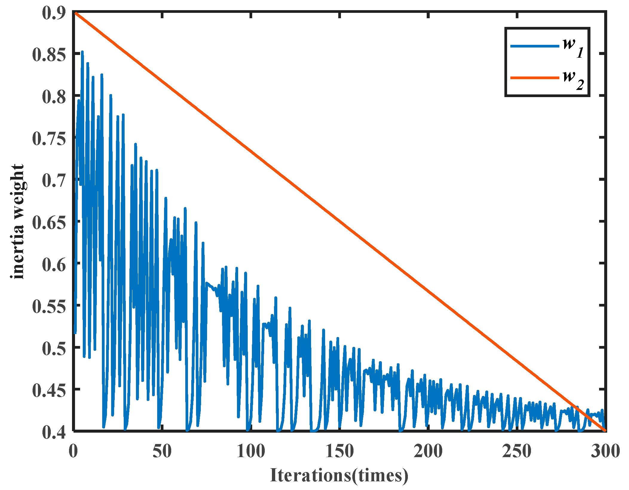
For the descending trend of different inertia weights shown in Figure 1, when the initial value of chaos $\alpha (0)=0.234$, the weight $w_1$ (with respect to COPSO) shows a dynamic variation throughout the iterations, which meets the requirements for dynamic values of $w$, while $w_2$ represents the linearly decreasing weight.

.

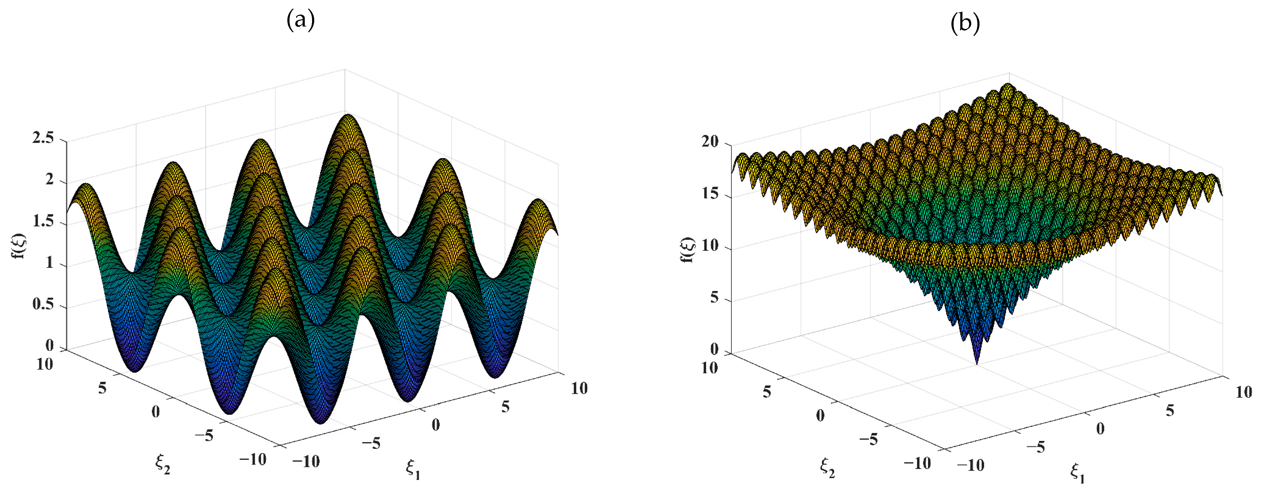
Two test functions (i.e., Griewank and Ackley function) with the same independent variable were chosen to evaluate the performance of different inertia weights. The Griewank function, with many widespread local minima (See Figure 2a), is usually employed to test the ability to escape from a local optimum and is defined as:

$$f(\xi )={\displaystyle \sum _{i=1}^D\frac{{\xi }_i^2}{4000}}-{\displaystyle \prod _{i=1}^D\cos \left(\frac{{\xi }_i}{\sqrt{i}}\right)}+1$$

(8)

where $D$ is the dimension. Here, $D=2$ and $-10\le {\xi }_i\le 10$ are chosen for testing.

The Ackley function, which is characterized by a nearly flat outer region and a large hole at the center (see Figure 2b), is used to test the global convergence and is defined as:

$$f(\xi )=-a\exp \left(-b\sqrt{\frac{1}{D}{\displaystyle \sum _{i=1}^D{\xi }_i^2}}\right)-\exp \left(\frac{1}{D}{\displaystyle \sum _{i=1}^D\cos (c{\xi }_i)}\right)+a+\exp \left(1\right)$$

(9)

where $D$ is the dimension. The variables for this test are set as $D=2$, $-10\le {\xi }_i\le 10$, $a=20$, $b=0.2$, $c=2\pi$, respectively.

As shown in Figure 2, note that both the Griewank function and Ackley function achieve the global minimum $f(\xi )=0$ under the condition of $\xi =(0,\dots ,0)$.

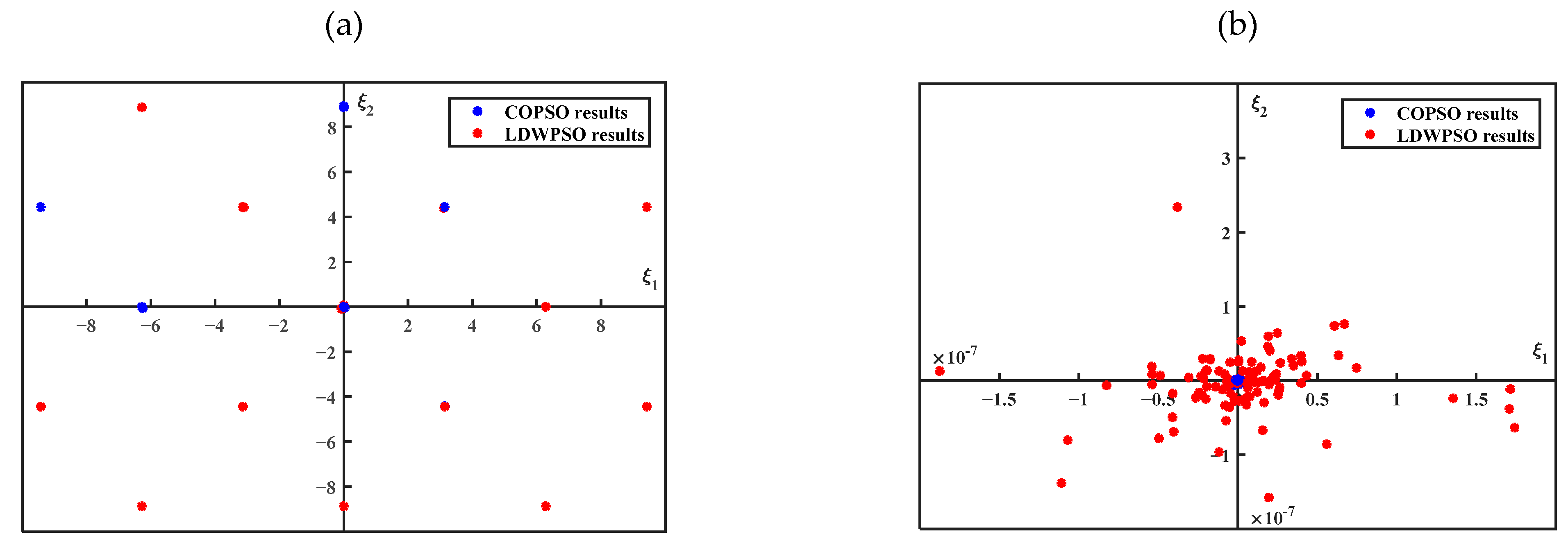
The PSO algorithms with two different inertia weights are employed to optimize the test functions. The maximum number of iterations and the number of particles for both weights are set as 100 and 10, respectively. The distribution of the particles is plotted in Figure 3 and the performance indicators for different inertia weights throughout the optimization process are listed in

Table 1. Comparison of different inertia weights for performance indicators.

Inertia Weight	Griewank Function		Ackley Function
	Mean Value of Fitness	Standard Deviation of Fitness	Mean Value of Fitness	Standard Deviationof Fitness
$w_1$	0.0075	0.0062	1.9252 × 10−9	2.9575 × 10−9
$w_2$	0.0083	0.0078	1.4285 × 10−7	1.6684 × 10−7

.

Figure 3 and Table 1 reveals that with more centralized distribution, a lower mean value, and a lower standard deviation, the $w_1$ strategy outperforms the $w_2$ strategy in its ability to escape from the local optimum and the global convergence rate, especially when the optimization problem is characterized by a more complicated and widespread local minima issue. Given the non-linear characteristics of the geophysical data inversion, especially for the on-ground GPR data, the test functions we chose would correspond better to the actual simulation circumstances of the on-ground GPR applications, which is also the motivation for this study in terms of improving the on-ground GPR inversion accuracy.

2.3. Improved Position Update Formula

The PSO algorithm is characterized by good portability and extensive practicability with respect to the inversion applications because it can optimize different practical problems by simultaneously adjusting the parameters of the velocity, inertia weight, and learning factors. Both searching and updating processes are performed based on different particles. When no additional constraints are imposed or applied, the dimensions in each particle generally do not affect each other; however, for geophysical data inversion, the subsurface media formation usually changes dynamically.

For this reason, the position updating formula of the PSO algorithm is modified to facilitate its adaptation into the changeable characteristics of the subsurface medium, allowing the effective integration of the forward modelling algorithm for GPR applications.

During the iterative process of the improved algorithm, both inversion and forward modelling use the same meshing technique with a square grid. Specifically, the improved algorithm iteratively takes each grid as a unit by employing the two-way travel time formula for EM waves, as well as the affinity between velocity and permittivity, in order to obtain the bilateral connection between $gbest$ and the corresponding fitting results according to:

$$t=\frac{2h\sqrt{\epsilon }}{c_0}$$

(10)

where $t$ is the two-way travel time, $\epsilon$ is the relative permittivity, $h$ is the depth of the object, and $c_0$ is the wave velocity in the vacuum.

Hence, the bilateral connection between model parameters of best particles together with the difference between forward recordings in different grids can be guaranteed; thus, based on the two-way travel time formula, the time corresponding to each grid can be calculated, as well as the ratio of the travel time to the total time that is recorded in the single trace, in order to establish the precise relationship between the observation parameters and the model parameters. In this way, the approximate initial direction in the search process can be obtained for particle inversion.

In addition, the optimal step size matrix $Q$ is further introduced and defined as a new ratio of the improved velocity variations for the next iterative update process. Note that $Q$ has the same dimensions as that of the particles in the PSO algorithm. Its individual elements represent the ratio of the corresponding forward recording time to the total time, and it is also treated as a constraint term in the improved algorithm. Compared with the full-space search of particles in the initial state, the constraint term can eventually provide the particles with an approximate direction choice to avoid falling into the local extremes.

To this end, the position update formula is improved by adding a new velocity variation:

$$x_{ij}(k+1)=x_{ij}(k)+\gamma v_{ij}(k+1)+Q_{ij}(k+1)\times v_{ij}(k+1)$$

(11)

where $\gamma$ is the control parameter of the improved velocity variations; $Q$ is the optimal step size matrix, which is multiplied by the velocity variations to obtain a new velocity variation at each position. These two parameters need to satisfy the basic relationship of $\gamma +\max (Q_{ij})\le 1$.

In this framework, by introducing the velocity variation term controlled by the step function, the improved position updating formula can effectively strengthen the bilateral connection to each position, as well as to each particle, thus guiding the searching process by using $gbest$ to improve the searching efficiency of the algorithm.

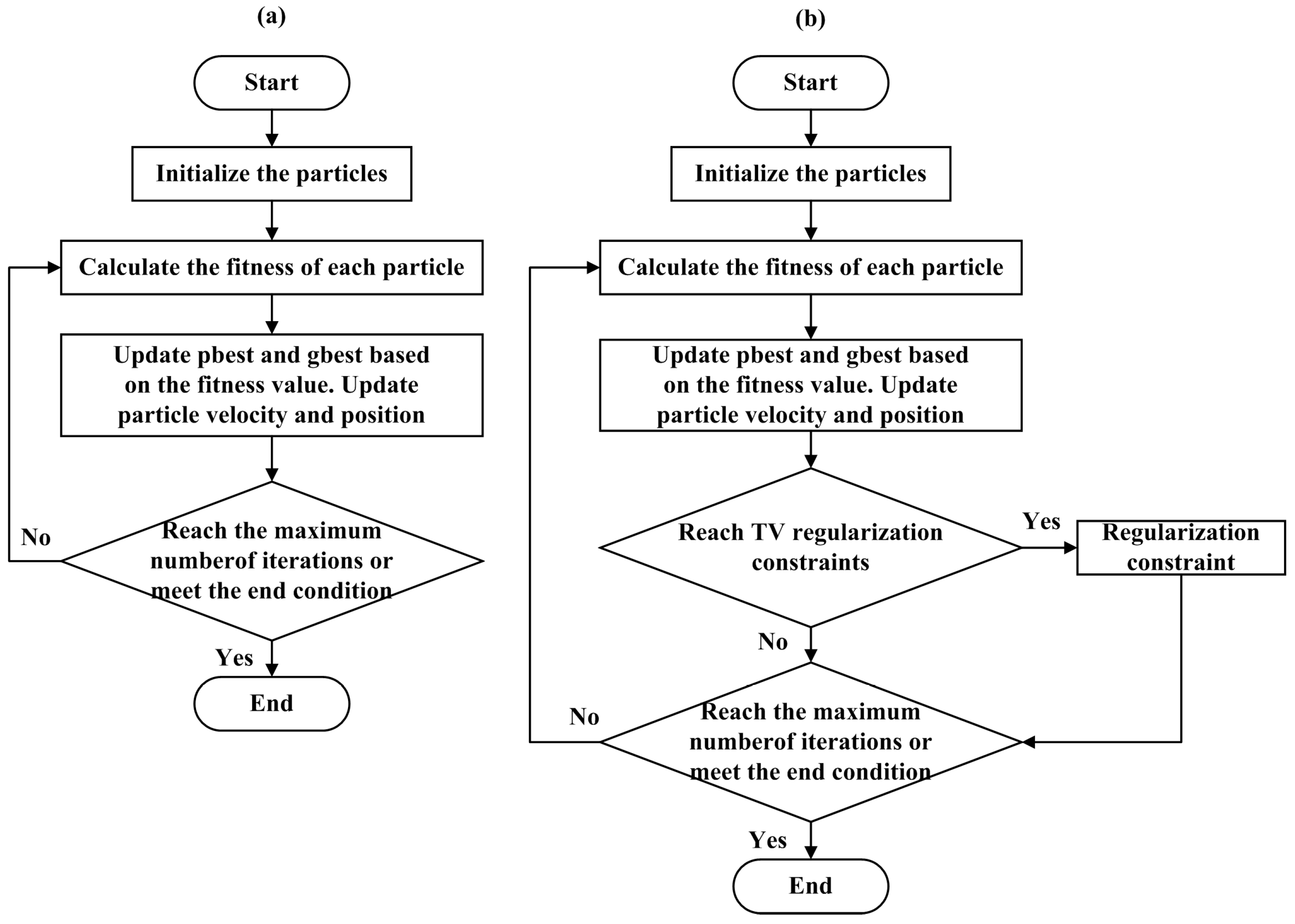
The basic PSO algorithm and improved PSO algorithm are graphically illustrated in Figure 4a,b, respectively.

2.4. TV Regularization Projection Constraints

In the iteration process, when the particle falls into the local optimum or when the fitness error drops slowly in the later iterations, a kind of disturbance term can be added to re-update the position of particles. By doing this, the algorithm is capable of not only escaping from the local optimum but also improving the inversion efficiency.

In order to solve the problem of premature convergence and slow convergence in the later stage, a TV regularization method based on the SB method is introduced to constrain the update process for the positions of particles [45]. The update process is then determined by the new judging process, which determines whether the particles meet the projection constraints for TV regularization. It is worth noting that the TV regularization constraint imposed in this study is essentially a disturbance term, which can facilitate the particles jumping out of the local minima.

In the case of two-dimensional complex model inversion, when the number of iterations reaches the maximum (generally set to 300), a better inversion result can be obtained. In the inversion experiment for the two-dimensional layered model, we found that when the number of iterations reaches 200, the fitness error has almost no change in the next 10 iterations.

The velocity and position update formulas can be improved as:

$$v_{ij}(k+1)=w(k)\times v_{ij}(k)+c_1{r}_1(pbes{t}_{ij}(k)-x_{ij}(k))+c_2{r}_2(gbes{t}_j(k)-x_{ij}(k))$$

(12)

$$x_{ij}(k+1)={{P}}_{\mathrm{c}}(x_{ij}(k)+\gamma v_{ij}(k+1)+Q_{ij}(k+1)\times v_{ij}(k+1))$$

(13)

where ${{P}}_{\mathrm{c}}(f)$ is the constraint function of the TV regularization with the following expression:

$${{P}}_{\mathrm{c}}(f)=\arg \underset{u}{\min }{\Vert \nabla u\Vert }_1+\frac{\lambda }{2}{\Vert u-f\Vert }_2^2$$

(14)

where the first term is the L1 norm of the gradient of model parameter $u$, which is the particle $x$ that satisfies the TV regularization constraint during the iterations (i.e., the relative permittivity of the model); the second term is the fidelity term, $\lambda$, which is the regularization factor. In this study, for the constraint condition, the global maximum point does not change within 10 iterations.

TV regularization uses the L1 norm of the model gradient as a regular term to smooth the model, which minimizes the total variation and thereby obtains the best model parameters. Consequently, the model can be smoothed without losing any detailed boundary features.

We show the flow charts of the COPSO and the TV-regularization-based improved particle swarm optimization (TVIPSO) algorithm in Figure 5.

2.5. Initial Model Construction

2.5.1. Multilayered Fluctuated Terrain Model

First, to highlight the importance of the suitability of the initial model to the inversion results, we built a multilevel fluctuated terrain model.

As shown in Figure 6a, the size of the model is set as $1\mathrm{m}\times 1\mathrm{m}$. Two fluctuated interfaces are specially designed at depths of 0.4 and 0.7 m. The relative permittivity levels of the three layers are set as 6.0, 9.0, and 12.0, respectively, while the conductivity of the background medium is set as 1 $\mathrm{mS}/\mathrm{m}$. The common offset gather (COG) function of the GPR simulation is performed using the FDTD method based on the unsplit-field convolutional perfect matching layer (UCPML) [64]. The grid interval is set as 0.01 m and the Blackman–Harris pulse with a central frequency of 900 MHz is used for forward calculation. The sampling interval and the time window are set as 0.04 and 16 ns, respectively. The trace interval is set as 0.01 m and a total of 100 traces are recorded. As the PSO algorithm is essentially an inversion algorithm that does not require the specific frequency, it is suitable for GPR inversion applications with different frequencies. The TVIPSO algorithm can also be adapted to on-ground GPR simulations of different frequencies.

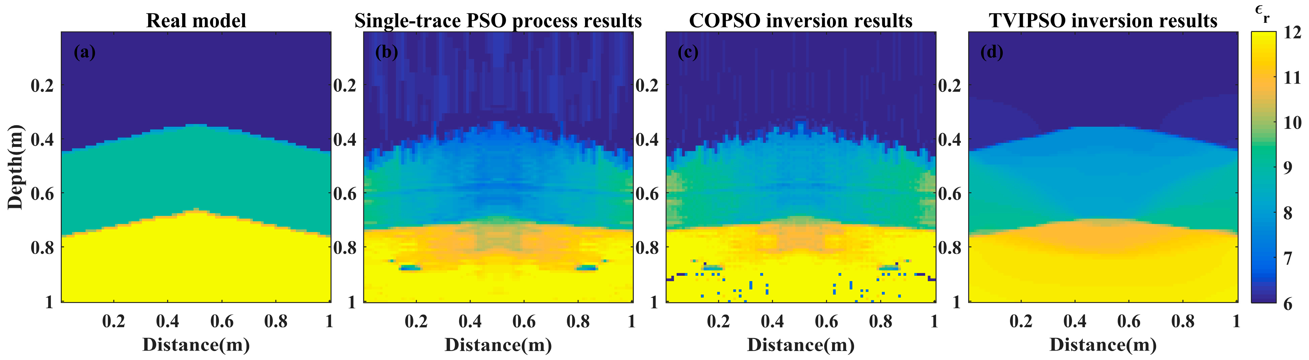
Both COPSO inversion and TVIPSO inversion are performed on the fluctuated terrain model and the grid meshing for the inversion is the same as that for the forward model. A random-layered model is firstly chosen as the initial model. In the initialization stage, each particle randomly generates the different layered models. The maximum number of iterations is 300 and the number of particles M is set as 30. The inversion result for several successive calculations is presented in Figure 6.

Figure 6b shows the inversion results of the COPSO algorithm. It turns out that no fluctuated interfaces are obtained. Figure 6c shows the inversion results of the proposed TVIPSO algorithm. Typically, the dielectric permittivity is concentrated between 8 and 10, which is quite different from the real model. In addition, some abnormal areas can also be found in the corners of the B-scan profile. In order to mitigate this, we continually increased the maximum number of iterations and the number of particles, but this situation did not improved. Conversely, this makes the inversion process rather time-consuming and the fitness error remains very high owing to the improper selection of the initial model together with the slow convergence in the later iteration process. In fact, this inversion failure is mainly because the parameters (i.e., randomly generated by each particle in the solution space) that correspond to the inappropriate initial model are too scattered. As a result, the inversion is prone to being trapped in the local optima, subsequently leading to inversion failure.

To avoid the inversion failure caused by the inappropriate initial model, we then improved the construction strategy of the initial model. Although the subsurface structure is generally continuous, it is inappropriate to generate rather random initial model parameters directly without using any prior information or applying any model constraints; hence, the rather random layered initial model can be improved by applying a relatively simple model constraint. For this, we refer to the same COG measurement configuration used for the transmitting and receiving antenna.

Firstly, we perform the PSO inversion of this multiple layered model at the selected measuring point to record the single-trace model parameters. Then, we splice the preliminary inversion results of the multitrace model parameters to construct the improved initial model; that is, the new initial model is constructed based on the single-trace PSO inversion profile.

2.5.2. Single-Trace PSO Process

The single-trace PSO process is carried out by using the same frequency component, the same type of excitation source, and the same COG configuration as that of the forward modelling for the fluctuated terrain model. The maximum number of iterations for inversion is set as $ite{r}_{max}$ = 300 and the number of particles M is set as 30. For 100 measuring points of the real fluctuated terrain model used for simulation, we select the first measuring point and a further 50 measuring points in total (one at each interval) to conduct the single-trace PSO inversion process.

On one hand, to calculate the fitness function, we choose the single-trace records corresponding to the current measuring point as the real model records for inversion. On the other hand, to on save calculation time, we perform the calculation starting from the measuring point at 0.01 m, with the trace interval set as 0.49 m; thus, every three traces are recorded. Note that the second record is selected as the inversion model record to calculate the fitness error, which means that the smaller the trace interval, the more accurate the results but the more time consuming the process.

As the subsurface terrain generally changes continuously, the model parameter differences between the two adjacent traces are small and the model parameter $gbest(N)$ obtained from the inversion of the N-th trace is substituted into the initialization stage of the inversion with the (N+2)-th trace; that is, it replaces one of the initialization particles and participates in the PSO inversion of the (N+2)-th trace.

A flow chart showing the construction of an appropriate initial model using single-trace PSO process is shown in Figure 7.

Note that 25 traces are utilized for this construction process. Table 1 shows the fitness error and mean square error (MSE) of the single-trace PSO inversion results of 25 traces, with an interval of one trace. Since the PSO algorithm is essentially an iterative random optimization process, random numbers can be added in the particle initialization process, as well as in the iteration process; hence, the result of each calculation or iteration is different. In this study, five inversions are performed for each trace. The data with the smallest fitness error is selected and is listed in

Table 2. Fitness error and MSE of the single-trace PSO process.

NO. of Traces	Fitness Error	MSE	NO. of Traces	Fitness Error	MSE
1	3.0740	0.3289	3	3.5434	1.2360
5	4.1044	0.2358	7	3.7464	1.6055
9	3.2042	0.2250	11	2.5701	1.0844
13	3.9843	0.1187	15	3.6789	2.1124
17	2.4247	0.5905	19	3.9378	1.6830
21	2.2695	0.4693	23	2.7522	1.0200
25	2.5650	0.4596	27	2.6660	0.6463
29	3.7318	0.8792	31	2.2974	0.4632
33	2.1940	0.9810	35	1.9960	0.3957
37	2.1235	1.1988	39	3.9018	2.1066
41	2.8597	1.0767	43	2.7987	0.7984
45	1.8708	1.4720	47	3.4056	1.3081
49	3.7103	1.5126

, which is used to obtain the initial model.

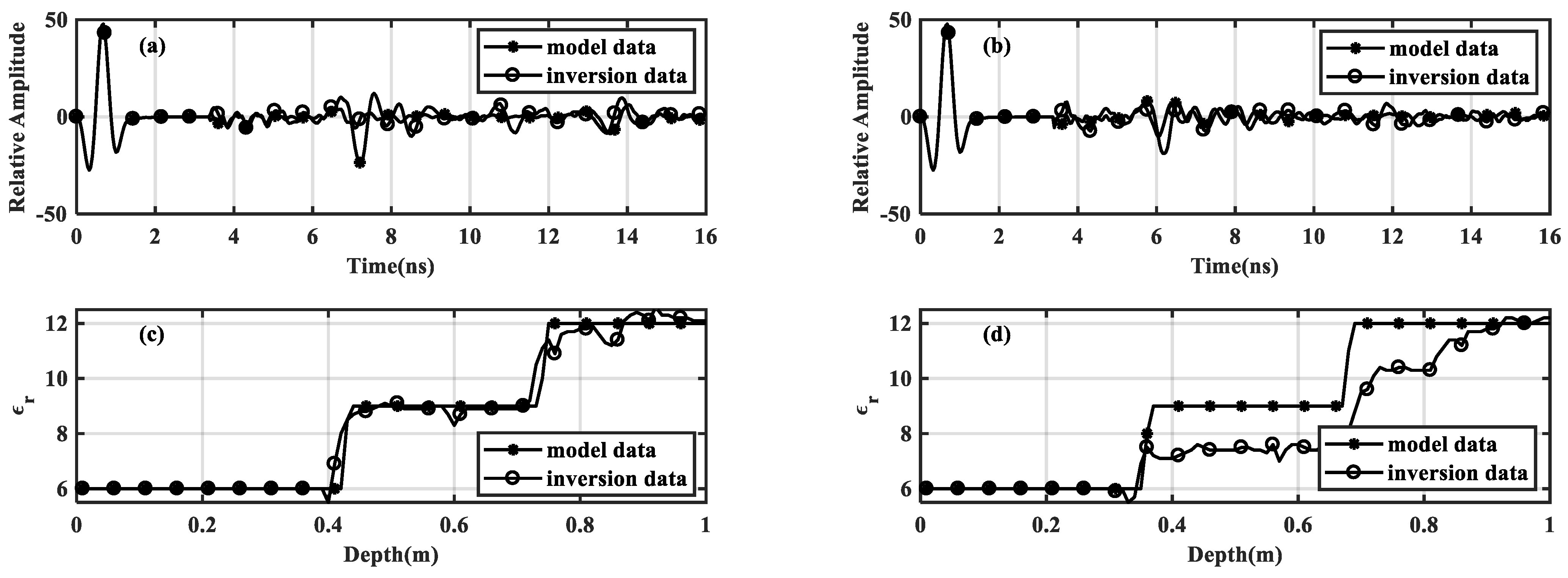
The 13th trace and the 45th trace are selected for comparison. The normalized relative amplitude and the dielectric permittivity are shown in Figure 8. It can be seen that: (1) the fitting degrees increase for both the amplitude recording and dielectric permittivity with the decreasing fitness error; (2) the correspondence between the depth information and the longitudinal trend of dielectric permittivity increases with the decreasing MSE. More importantly, by using this process, we can obtain a more appropriate initial model in a faster time.

It should be pointed out that this single-trace-based strategy is also applicable for the other gather datasets because the targeted trace selection is more oriented toward enhancing the suitability of the initial model, especially if borehole data are available.

3. Results and Discussion

3.1. Fluctuated Terrain Model

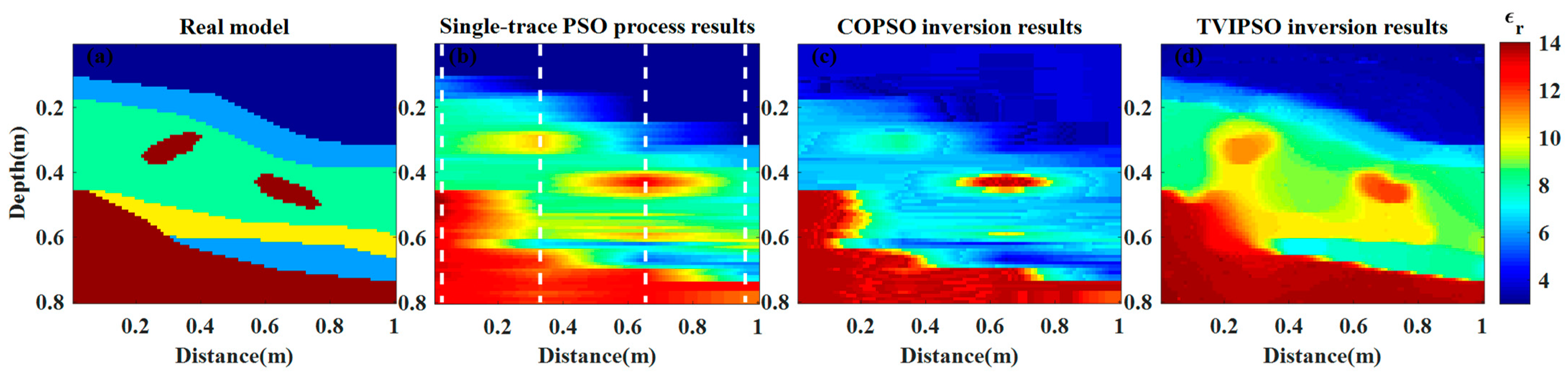
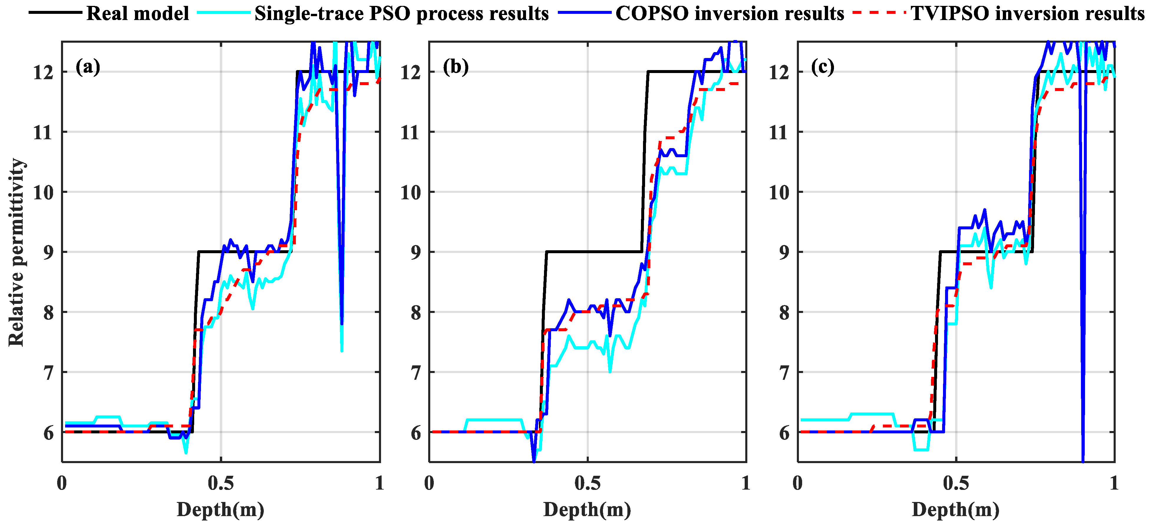
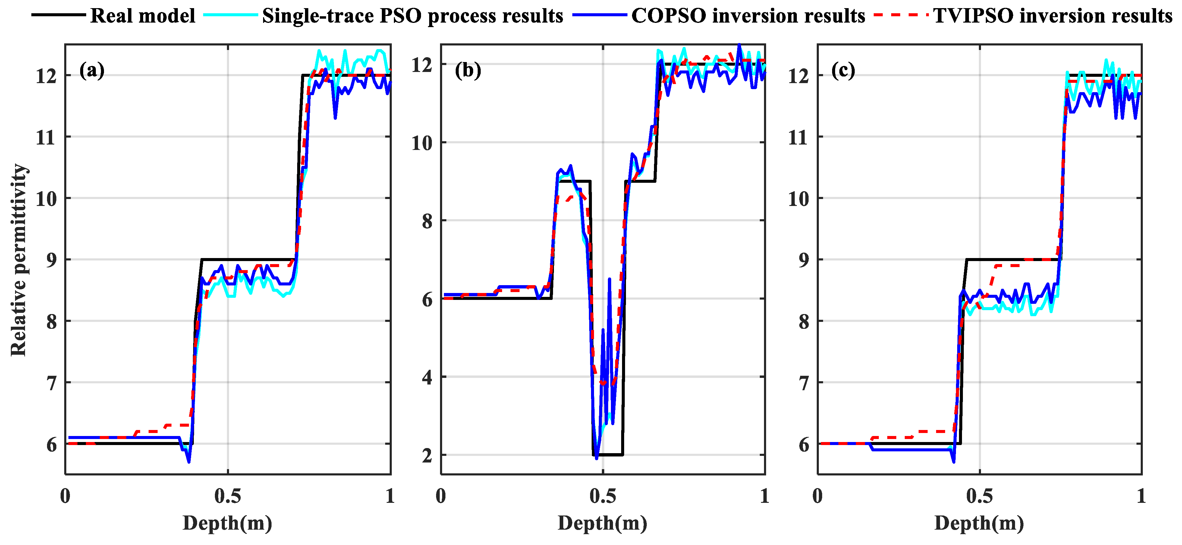
According to step 2.5, the trace-combined initial model is constructed, which is shown in Figure 9b. Then, this initial model is employed as one of the initializing particles to perform the COPSO inversion and the TVIPSO inversion. The maximum number of iterations is set as 300, the number of particles M is set as 30, and the other parameters remain the same. Figure 9c,d show the inversion results for the two algorithms. The detailed dielectric permittivity inversion curves at three horizontal positions (i.e., at distances of 0.16, 0.56, and 0.94 m) are further expatiated and are plotted in Figure 10.

In these B-scan images, it can be seen that apart from the local region near the two fluctuated interfaces where the permittivity from the TVIPSO method is slightly lower than that of the real model, the proposed TVIPSO method outperforms the COPSO algorithm significantly. Compared with the inversion results from the COPSO algorithm, the fluctuated terrains from the TVIPSO method are more consistent with the real model with the same number of inversion iterations. The advantages include the fit of the parameters, the continuous distribution of the dielectric permittivity, the high-resolution images generated of two fluctuated interfaces, and the better convergence rate, particularly the high stability of the iterative random optimization process.

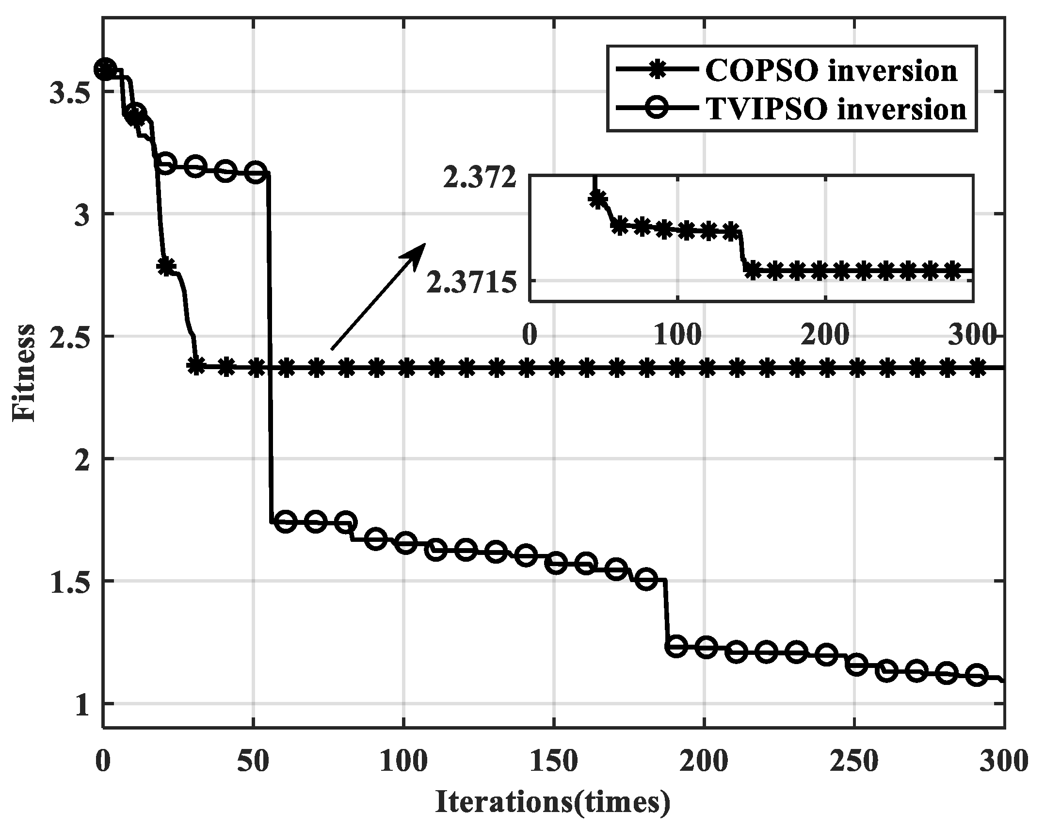
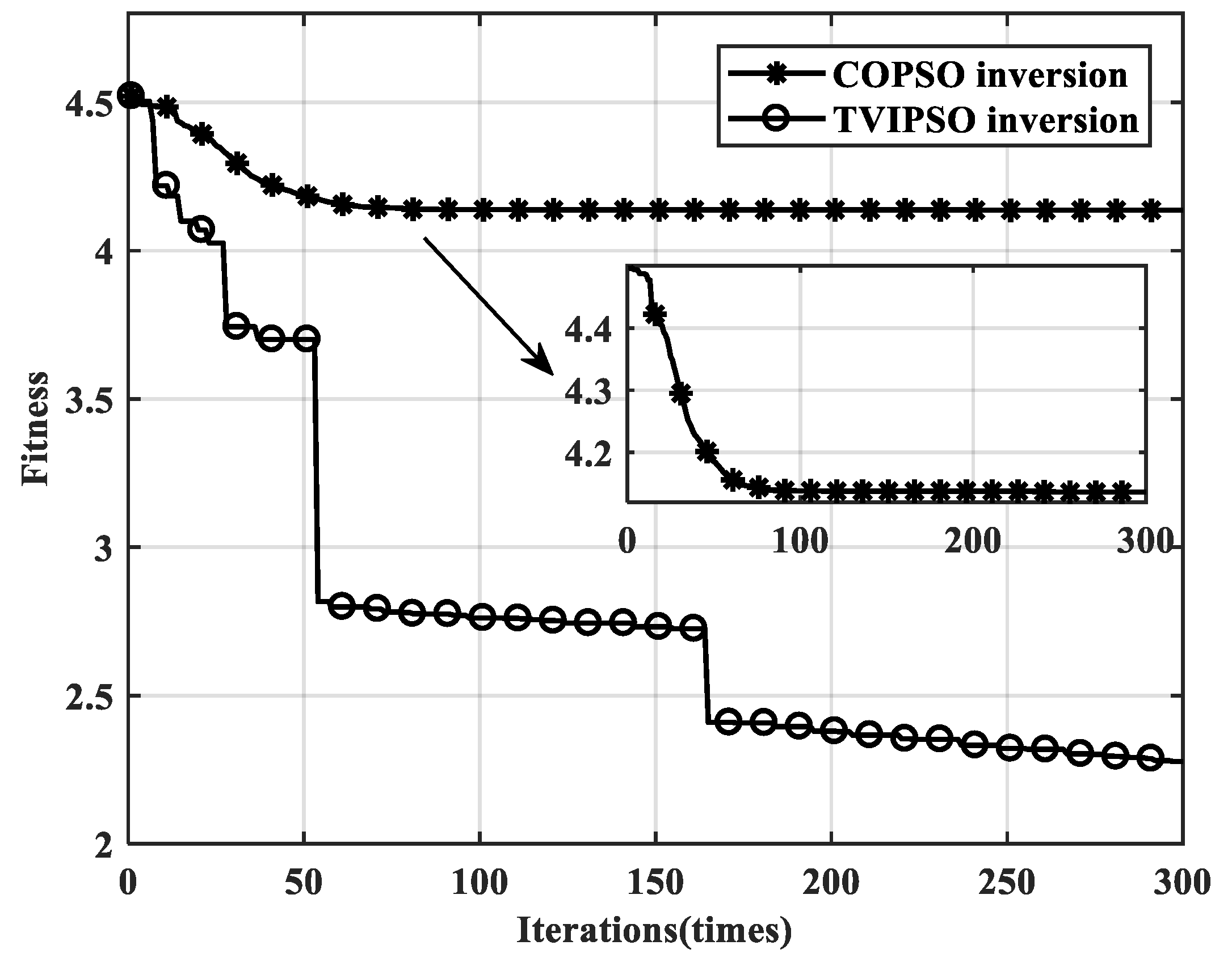
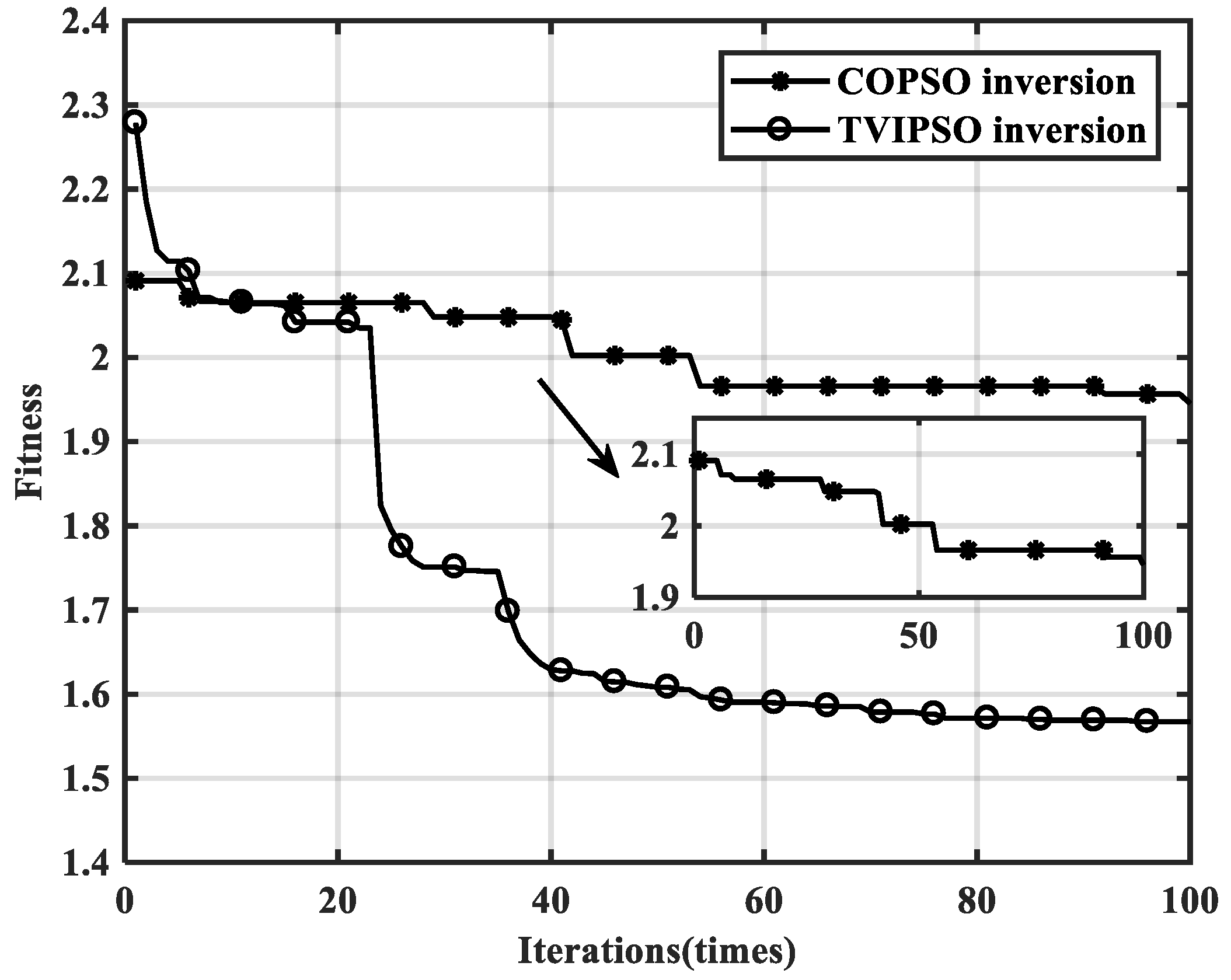
Figure 11 shows the convergence curves of the fitness functions with the two algorithms, while

Table 3. Comparison of iteration details for the two PSO algorithms.

Inversion Method	Fitness Error	MSE	MAPE	RMSE
Initial model	3.5868	0.7749	6.31%	0.8803
COPSO inversion results	2.3715	0.6611	4.44%	0.8131
TVIPSO inversion results	1.0921	0.3841	3.96%	0.6198

lists the iteration details of two PSO inversion algorithms.

As shown in Table 3 and Figure 11, with the same initial model, the TVIPSO algorithm exhibits a lower fitness error, mean square error (MSE), mean absolute percentage error (MAPE), and root mean squared error (RMSE) compared to the COPSO algorithm. More importantly, after two obvious convergence drops, the final fitness error of the TVIPSO method is reduced to 1.0921, whereas the COPSO method shows a divergent state after 32 iterations and its fitness error is maintained at 2.3715 (at twice the fitness error of TVIPSO).

The most important reason for this outperformance of the TVIPSO algorithm is that the regular TV term can optimize the intercorrelations among different particles, helping to avoid the “blind flight” occurrences of particles and making it capable of jumping away from the local extremes to guarantee the inversion accuracy. Additionally, both the new velocity variations and optimal step-size matrices are helpful in speeding up the convergence rate of the algorithm (see the late-stage curve in Figure 11).

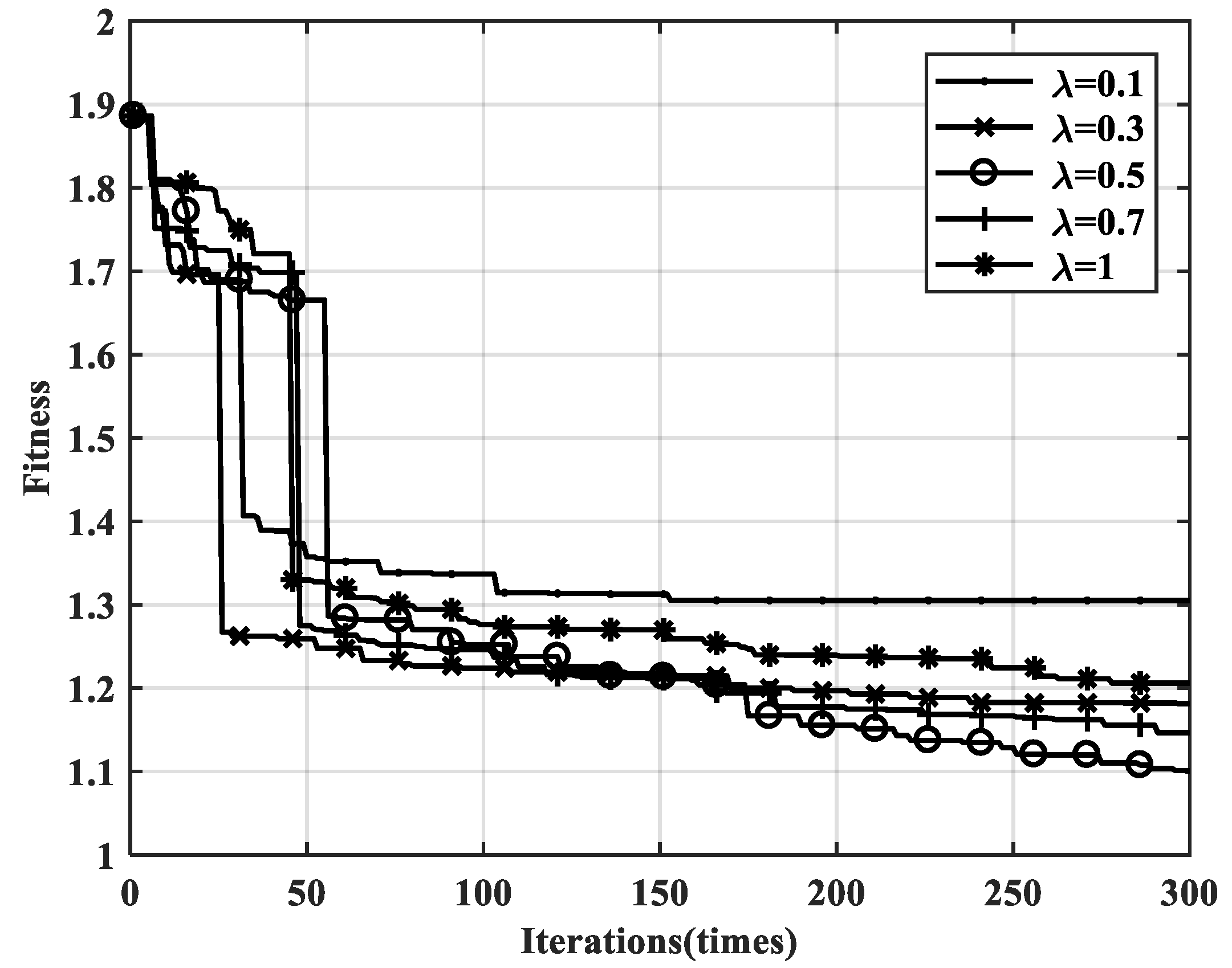
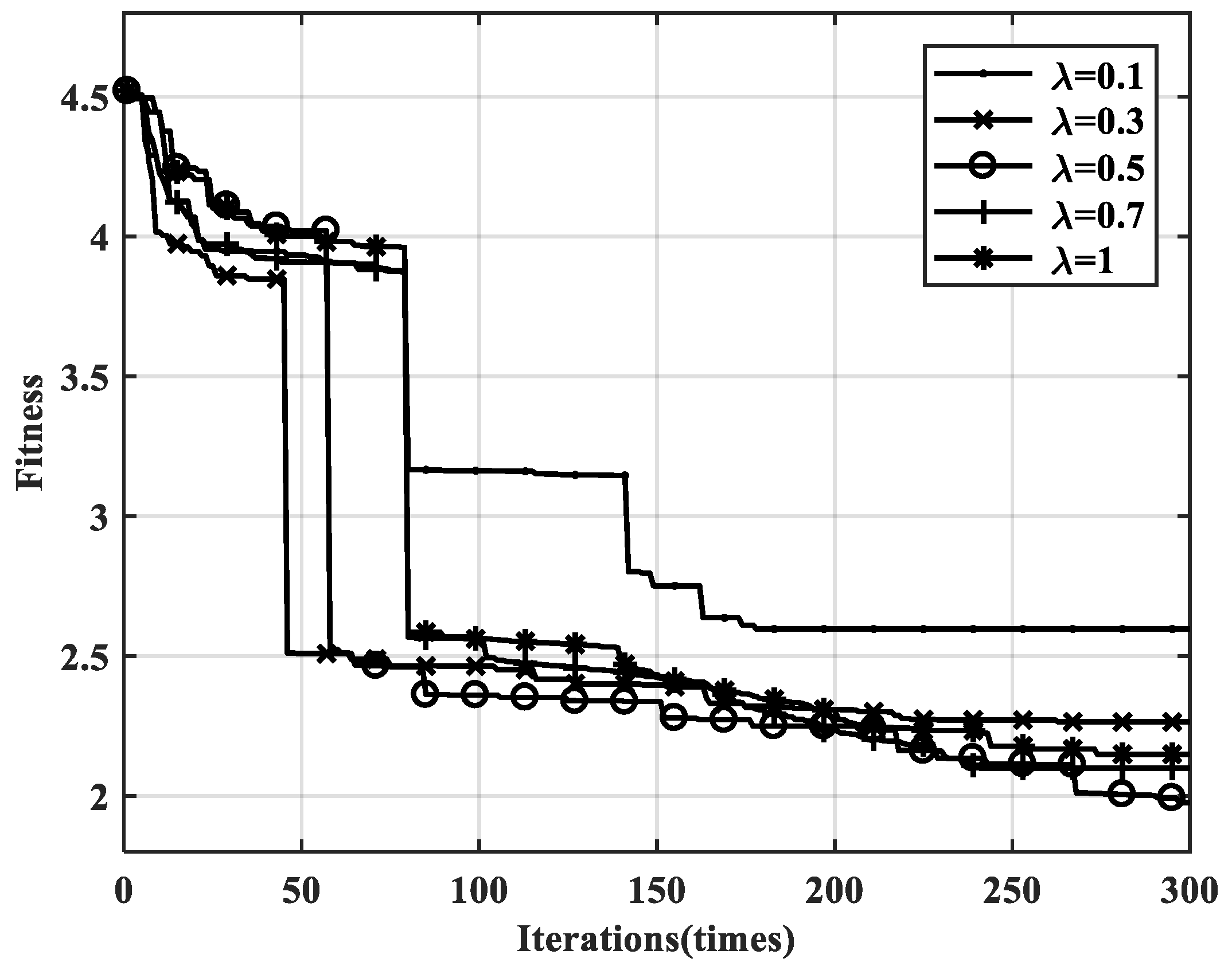
Figure 12 shows the impacts of the different regularization factors on the fitness error of the improved PSO algorithm with the same number of iterations. Here, five regularization factors are investigated and each factor is subjected to three consecutive inversion calculations, then the minimum fitness error is recorded.

As shown in the convergence curves, when λ is set to 0.5 in this case, the smallest fitness error for the inversion is obtained; in addition, the curve manifests a continuous convergence state, even in the later stages after 300 iterations. When λ is set to 0.1, the algorithm falls into another local extreme, which may result from the excessive smoothing process, meaning the convergence rate is quite slow and the optimization iteration is actually terminated in the middle stage. When λ is set to 1, the regular TV term shows a weak constraint on the algorithm and the amount of variation in the particles is relatively small, which also results in a slow decline with respect to fitness. When the regularization factor is set to 0.1, 0.3, or 0.7, the convergence trends are also terminated at different iterations in the late stages.

In this sense, the regularization factor for TVIPSO inversion should be selected according to the different medium components or different meshing sizes of the model. Regularization factors that are too large or too small may cause the algorithm to fall into the local extremes or may result in premature convergence or termination in the middle or later stages of the iteration.

3.2. Abnormality-Embedded Fluctuated Terrain Model

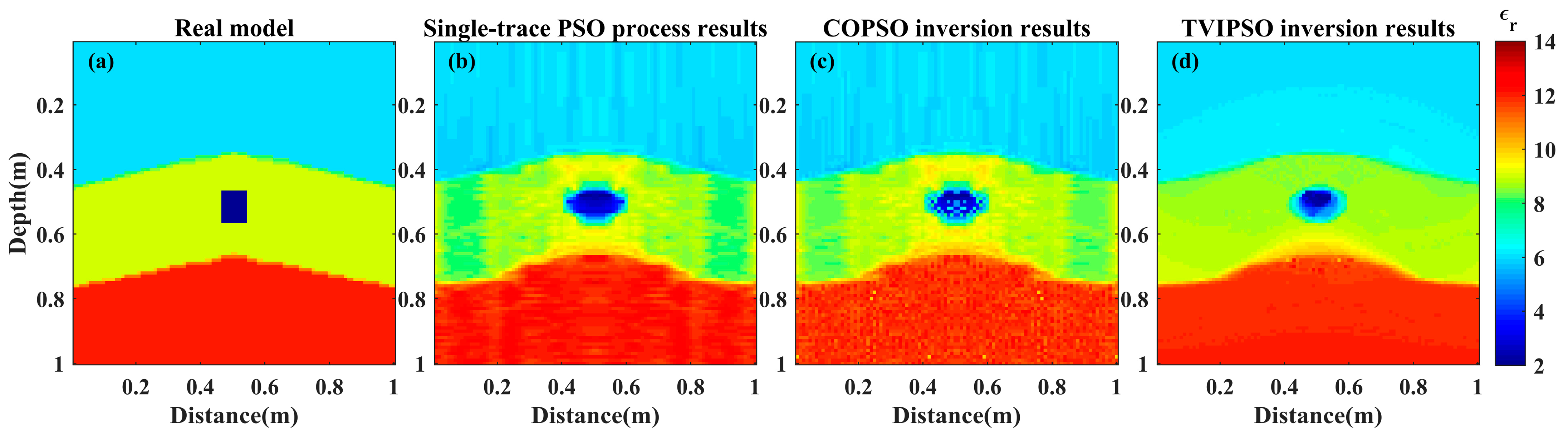
In order to further verify the practicability of the proposed method with applications to complex models, an inversion test is performed, in which a rectangular abnormal body measuring 0.08 × 0.1 m and with a dielectric permittivity of 2 is embedded in the second layer of the former fluctuated terrain model at a depth of 0.47 m, as shown in Figure 13a.

The Blackman–Harris pulse with a main frequency of 900 MHz is also chosen as the excitation source. The sampling time interval and the time window length are set as 0.03 and 16.5 ns, respectively. The measurement configuration remains the same as that of the former test.

Figure 13b shows the initial model constructed using the fast single-trace PSO process. The COPSO inversion and TVIPSO inversion are then tested on the same initial model. The maximum number of iterations is also set as 300 and the number of particles M is set as 30, while other optimization iteration parameters remain the same. Figure 13c,d show the inversion results of the two algorithms. Figure 14 shows the detailed dielectric permittivity inversion curves at three horizontal positions (i.e., at distances of 0.22, 0.53, and 0.97 m, respectively).

As shown in Figure 13 and Figure 14, both PSO inversion algorithms can fit the position information of the two fluctuated interfaces, as well as the location of the abnormal body; however, the apparent blurring problem is found in the COPSO inversion results (see Figure 13c), especially regarding the morphology reconstruction and the fine outline of the abnormal body. Comparatively, the TVIPSO method shows promising results as it effectively solves the blurring problem using the regular TV term; note the improved reconstruction accuracy and increased number of discernible details of not only the two fluctuated interfaces but also of the morphology of the rectangular abnormal body.

In addition, the permittivity inversion curve for the TVIPSO algorithm at three different positions are better fitted with that of the real model, as presented in Figure 14a,c; it is not an oscillated curve such as the curve the COPSO algorithm shows.

Table 4. Comparison of the iteration details for the two inversion methods.

Inversion Method	Fitness Error	MSE	MAPE	RMSE
Initial model	4.5210	0.3760	4.03%	0.6132
COPSO inversion results	4.1364	0.3476	4.14%	0.5896
TVIPSO inversion results	2.2778	0.2459	3.55%	0.4959

lists the iteration details for the two PSO inversion methods. Figure 15 shows the convergence curves of fitness functions for the two algorithms.

From the two convergence curves and the iteration details, it can be seen that although the TVIPSO algorithm did not reach the TV regularization constraint condition within the previous 50 iterations, the newly added position update formula shows a better convergence rate during the initial iteration stage compared with the COPSO algorithm. After 50 iterations, the convergence rate of the COPSO algorithm is still quite slow and the neighborhood converge limits the searching to a local optimum prematurely during the middle stage (i.e., 100 iterations). As a result, the iteration is finally converged and terminated to the former local optimum with a rather large fitness error.

In contrast, the TVIPSO algorithm shows a continuous drop convergence state in searching for the global optimal solution across the total of 300 iterations. More importantly, the calculation of the TVIPSO process goes through two obvious steepening drop periods in the fitness error process. The final fitness error is approximately half that of the COPSO algorithm.

It can be concluded that for the same inversion problem and the same initial model considered, the TVIPSO algorithm outperforms the COPSO algorithm in terms of the inversion efficiency as it capable of converging to the global optimal solution for the desired inversion accuracy with less iterations.

Figure 16 presents the detailed impacts of the different regularization factors on the fitness error of the improved PSO algorithm. Figure 17 shows a comparison of the inversion results with the regularization factors set to 0.1, 0.5, and 0.7, respectively. It demonstrates that when the regularization factor is set to 0.5, the fitness error of the inversion is the smallest, while the curve shows the desired continuous drop convergence trend throughout the 300 iterations. The inversion accuracy is verified by the precise morphology of the rectangular abnormal body, as well as the outline continuities of the second fluctuated interface.

3.3. Complicated Inner-Interface Model with Noisy Dataset

For further testing of the robustness of the proposed method, we designed a complicated inner-interface model with a noisy dataset added. The complexity of the model is shown in Figure 18a. The model consists of 80 × 100 quadrilateral grids. The variation range of the permittivity of the model media is set between 3 and 14, where the upper layer represents the dry sand layer of the surface, the second layer is thin layer measuring 0.08 m in thickness, two irregular abnormal bodies are found in the third layer with high relative permittivity, and a low-permittivity lens layer (at 0.6 m depth) is located on the lower right of the model, beneath which a soft interlayer is specially designed at a depth of 0.7 m.

The excitation employs the Blackman–Harris pulse with a central frequency of 900 MHz. The sampling interval and the time window are set to 0.03 and 15 ns, respectively. The observation mode is the same as the aforementioned fluctuated terrain model. Figure 18b shows the initial model that constructs the single-trace PSO process. Note that the initial model here is constructed by extracting only four traces in the observation records.

The number of particles and the maximum number of iterations are set as 30 and 100, respectively. The mean absolute relative error (MARE) is computed and selected as the fitness function to solve the inversion problem.

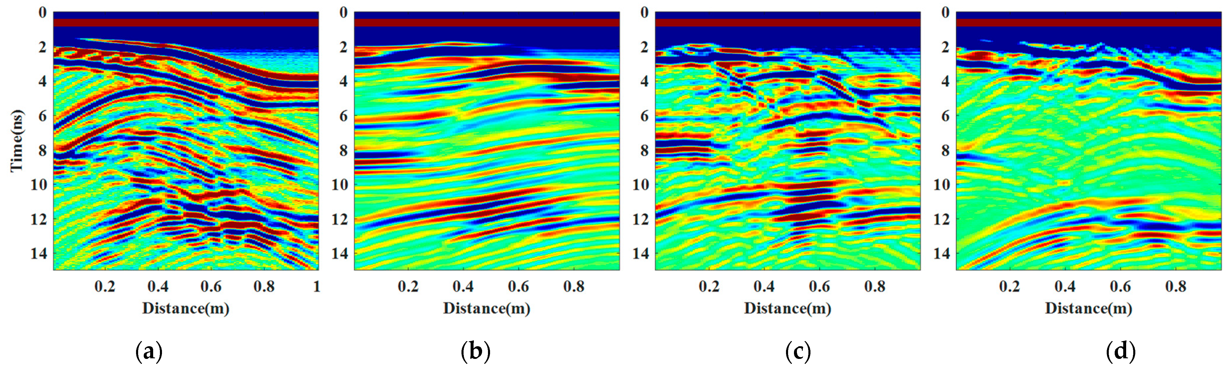
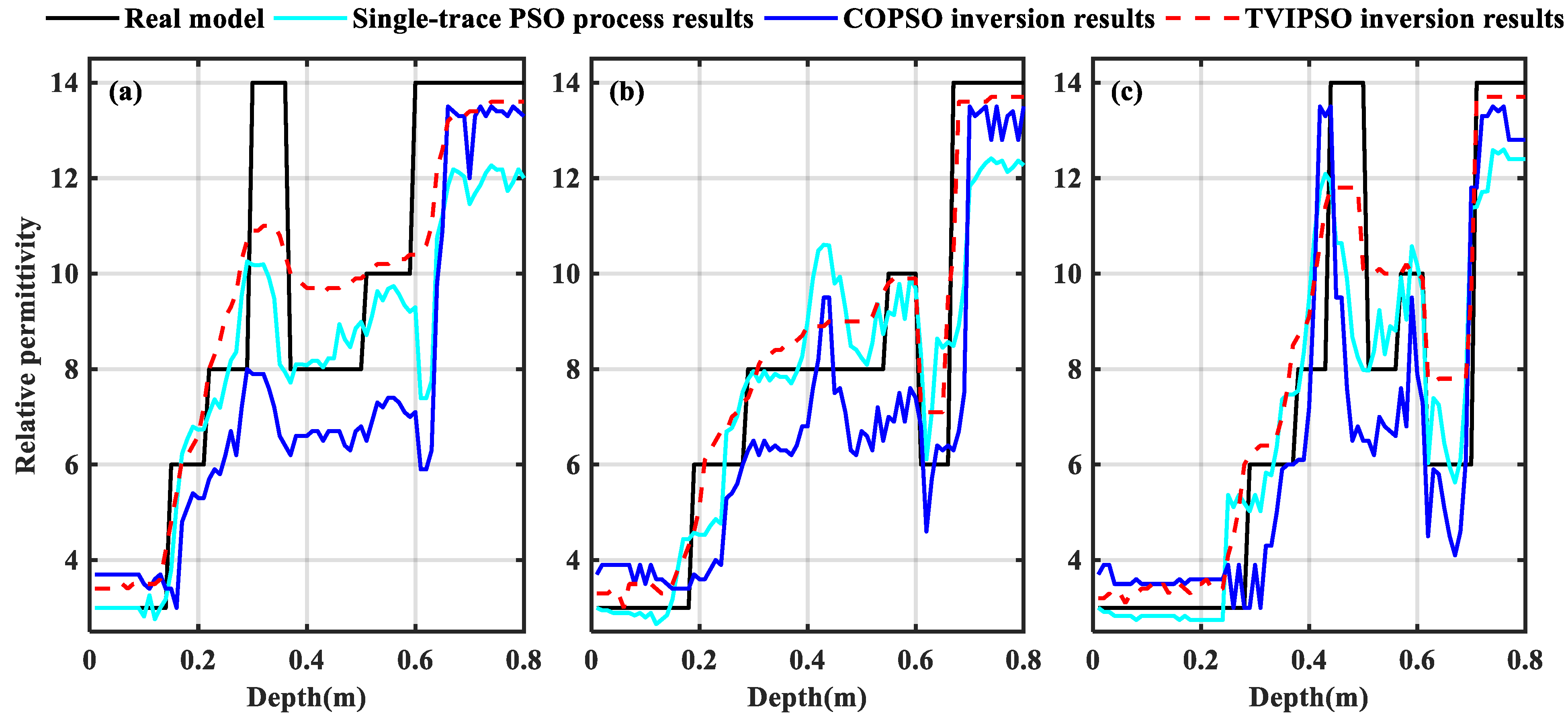
Figure 18c,d show the inversion results for the two algorithms. Figure 19 presents a comparison of the observation records with 10% noisy data added, the forward records of initial particles, and the forward records corresponding to the inversed models of the two PSO algorithms. Figure 20 shows the detailed permittivity inversion curves at three horizontal positions (i.e., at distances of 0.30, 0.50, and 0.70 m, respectively).

Table 5. Comparison of iteration details for the two inversion algorithms.

Inversion Method	Fitness Error	MSE	MAPE	RMSE
Initial model	2.0993	2.3438	11.33%	1.5310
COPSO inversion results	1.9539	4.1523	19.60%	2.0377
TVIPSO inversion results	1.5674	1.4685	12.55%	1.2118

lists the iteration details for the two PSO inversion algorithms.

From the comparison results, it can be seen that the searching tendency for COPSO is very sensitive to the high permittivity regions; that is, in terms of the driving force searching in the COPSO algorithm, the high-permittivity region has a more misleading driving force in the searching process when compared to the low-permittivity region, which leads to inversion ambiguity and inversion failure in the low-permittivity region, as shown in Figure 18c and Figure 20.

In contrast, the TVIPSO algorithm properly solves the search sensitivity problem regarding the high-permittivity region imaging. Although the value shows a small deviation from the real model, the reconstruction accuracy of the TVIPSO algorithm dramatically outperforms the COPSO algorithm. Note that remarkable improvements are not only revealed in the accurate reconstruction of the abnormal body location, but also in the fine inversion of the low-permittivity region of the complicated model. To a certain extent, the COPSO algorithm actually falls into the local optima in this complicated model (as shown in Figure 21).

4. Conclusions and Outlook

In this study, to improve the precision and efficiency of the PSO inversion for complex models, a new algorithm was proposed for on-ground GPR data inversion based on the improved velocity variations, the optimal step size matrices, and the total variation regularization technique.

First, we developed a single-trace-based process to construct the initial model for PSO inversion, with a fast iterative process and simple programming, which is beneficial and convenient for accelerating the implementation of the GPR full-waveform inversion.

Then, the chaotic oscillation PSO algorithm was improved by adding the new velocity variations and optimal step-size matrices to strengthen the bilateral connection between different particle positions, as well as the dimensions in the particles. By doing this, the searching space of the random particles can be significantly reduced to mitigate the premature convergence and slow convergence rate, meaning the blindness in the search process can be avoided.

Finally, the total variation regular term was proposed and applied in the optimization iteration process, which prevents the optimization search from leaving the accurate region. In particular, the proposed constraint-oriented inversion strategy not only optimizes the smoothness of the reconstructed image but can also improve the resolution of the edge details.

Both the fluctuated terrain model and complicated inner-interface model were tested to verify the practicability of the proposed algorithm. The results demonstrated that both the fitness error and MSE of inversion decreased, while the global rate of convergence and discernible details of the anomalies were also improved.

It is needs to be emphasized that the regularization factor for the proposed algorithm should be selected depending on the medium component and the meshing used for the on-ground GPR inversion problem.

More importantly, performing adaptive adjustments regarding the parameters setting still requires substantial complicated model testing, especially for the inversion efficiency analysis when more control parameters are considered. There are currently ongoing studies focusing on dispersion models with PSO inversion for on-ground GPR inversion. Additionally, comparing the TVIPSO algorithm with other inversion approaches such as genetic algorithm will be another aim of our future studies on GPR inversion applications.

The next study will also focus on integrating previous research with a realistic validation of the proposed method. In order to make the simulation effects better correspond to actual situations, we also consider it is necessary to take into account the antenna coupling effect in the in-site field test, for instance using the complicated hierarchical model in a sand tank experiment.