Abstract
Multispectral imaging using Unmanned Aerial Vehicles (UAVs) has changed the pace of precision agriculture. Actual evapotranspiration (ETa) from the very high spatial resolution of UAV images over agricultural fields can help farmers increase their production at the lowest possible cost. ETa estimation using UAVs requires a full package of sensors capturing the visible/infrared and thermal portions of the spectrum. Therefore, this study focused on a multi-sensor data fusion approach for ETa estimation (MSDF-ET) independent of thermal sensors. The method was based on sharpening the Landsat 8 pixels to UAV spatial resolution by considering the relationship between reference ETa fraction (ETrf) and a Vegetation Index (VI). Four Landsat 8 images were processed to calculate ETa of three UAV images over three almond fields. Two flights coincided with the overpasses and one was in between two consecutive Landsat 8 images. ETrf was chosen instead of ETa to interpolate the Landsat 8-derived ETrf images to obtain an ETrf image on the UAV flight. ETrf was defined as the ratio of ETa to grass reference evapotranspiration (ETr), and the VIs tested in this study included the Normalized Difference Vegetation Index (NDVI), Soil Adjusted Vegetation Index (SAVI), Enhanced Vegetation Index (EVI), Normalized Difference Water Index (NDWI), and Land Surface Water Index (LSWI). NDVI performed better under the study conditions. The MSDF-ET-derived ETa showed strong correlations against measured ETa, UAV- and Landsat 8-based METRIC ETa. Also, visual comparison of the MSDF-ET ETa maps was indicative of a promising performance of the method. In sum, the resulting ETa had a higher spatial resolution compared with thermal-based ETa without the need for the Albedo and hot/cold pixels selection procedure. However, wet soils were poorly detected, and in cases of continuous cloudy Landsat pixels the long interval between the images may cause biases in ETa estimation from the MSDF-ET method. Generally, the MSDF-ET method reduces the need for very high resolution thermal information from the ground, and the calculations can be conducted on a moderate-performance computer system because the main image processing is applied on Landsat images with coarser spatial resolutions.
1. Introduction
The world population is projected to reach 9.7 billion by 2050 [1]. Satisfying the food demand of such a population is a big challenge. FAO estimated that food production needs to double by 2050, which would require a massive amount of water. The challenge is that water is already scarce and agriculture alone accounts for more than 70% of total freshwater withdrawals [2]. Therefore, there is an urgent need to produce more food with less water, which can only be achieved by improving water use efficiency in the largest water consuming sector.
Current remote sensing technologies provide an opportunity to monitor water consumption over large areas in a cost-effective way. They offer an important decision support tool with lots of potential for growers and stakeholders.
Improved sensors onboard Unmanned Aerial Vehicles (UAVs) and remote sensing methods have given us the ability to observe fields with detail and capture stress and evapotranspiration (ET) at the plant level [3]. Very high spatial resolution maps are essential for food optimization, crop production, irrigation, and fertilization management in precision agriculture [4], and the relatively lower spatial resolution of satellite images are not capable of accurately accounting for spatial heterogeneity in topography, soils, and vegetation [5].
Several satellite-based remote sensing approaches have been developed for mapping actual ET (ETa) over agricultural areas. The main one-source energy balance algorithms include Surface Energy Balance Algorithm for Land (SEBAL) [6], Surface Energy Budget System (SEBS) [7], and Mapping Evapotranspiration at High Resolution with Internalized Calibration (METRIC) [8,9]. One of the most prominent stages of calculating ETa from one-source algorithms is identifying anchor pixels. Very high spatial resolution images commonly lack pixels superimposed over well-watered vegetation as the cold pixel due to the limited areas covered by cameras onboard UAVs [10]. Ramírez-Cuesta et al. [10] made an effort to identify anchor pixels based on the relationship between land surface temperatures (LSTs) derived from Landsat and UAV images.
The two-source algorithm [11] was developed to estimate heat transfer for soil and vegetation separately, excluding the need for anchor pixels selection. Several studies show the successful implementation of the two-source algorithm based on very high spatial resolution imagery [3,12,13]. Some researchers have made use of different techniques for enhancing ETa estimates of UAV images. Torres-Rua et al. [14] took deep learning techniques into account for ETa estimation using a two-source algorithm based on thermal information obtained from a UAV. Aboutalebi et al. [15] incorporated point cloud products derived from UAV images into remote-sensing-based ETa estimation models and improved their results. Zipper et al. [16] developed the High Resolution Mapping EvapoTranspiration (HERMET), specifically designed for UAV images, by separating vegetation and soil. However, all of these are in critical need of thermal information from the surface obtained using cameras onboard UAVs.
Removing thermal cameras from UAVs can reduce the devices’ cost, but ETa calculation would be more challenging. Several studies have demonstrated that satellite-derived potential ET and ETa can be estimated without the use of thermal bands by taking into account the FAO Penman-Monteith equation and different crop coefficient estimation methods [17,18,19]. The Simple Algorithm For Evapotranspiration Retrieving (SAFER) was developed specifically in case of ETa, coupling remote sensing parameters calculated using multispectral bands and agrometeorological data for ETa calculation [20]. Data fusion methods can also be beneficial for high resolution ETa mapping with shorter intervals between images. There have been several data fusion methods for sharpening thermal images such as TsHARP [21], SADFAT [22], and TS2uRF [23]. Several studies have focused on LST and ETa sharpening for enhanced resolution ETa calculation [4,24,25], but needless to say all of these focused on high- and moderate-resolution satellites equipped with thermal bands. Nevertheless, there are widely used operating satellites and UAVs which lack the ability to capture images in the thermal portions of the spectrum. Hence, some researchers have taken advantage of data fusion methods based on the relationship between Moderate Resolution Imaging Spectroradiometer (MODIS) LST product and Vegetation Indices (Vis) in order to eliminate the need for thermal bands when calculating potential ET using Landsat 8 and Sentinel-2 [26,27]. Xue et al. [28] proposed a modified data mining sharpener approach to estimate a 30-m high temporal resolution LST by fusing ECOSTRESS/VIIRS data with harmonized Landsat and Sentinel-2 surface reflectance data. Also, a few studies have focused on combining Sentinel-2 (multispectral) and Sentinel-3 (thermal) images by making use of data fusion for ETa estimation [29,30]. However, the combination of satellite and UAV data through data fusion approaches for ETa estimation still remains untouched.
The relationships between ETa and VIs are strong [31,32] and have proved to be a great tool for estimating satellite-based ETa [33,34]. The Normalized Difference Vegetation Index (NDVI) [35] is the most commonly used VI, and has been further improved as the Soil Adjusted Vegetation Index (SAVI) [36] and Enhanced Vegetation Index [37] to remove the effects of soil background and atmosphere, respectively. Also, since the Shortwave Infrared (SWIR) portion of the spectrum can relate surface moisture to optical reflectance [38], two water indices, namely, the Normalized Difference Water Index (NDWI) and Land Surface Water Index (LSWI) [39,40], have been used for detecting moisture variability of surface. It is speculated that these indices may be beneficial for monitoring surface ETa rates.
The objective of this study was to exclude thermal camera requirements for UAV-based ETa mapping using the modified TsHARP algorithm specifically designed for ETa sharpening, herein referred to as the multi-sensor data fusion approach for ET estimation (MSDF-ET). To achieve this goal, a UAV equipped with multispectral and thermal cameras and Landsat 8 images were used in consideration of the following steps: (1) perform Landsat 8-based ETa calculation using the METRIC algorithm and subsequently the reference ET fraction (ETrf); (2) find a linear regression equation based on the relationship between different VIs and ETrf at the Landsat 8 resolution; (3) build a Bias image for each Landsat 8 overpass; (4) apply the algorithm to UAV images and calculate the ETrf at a very high spatial resolution; (5) visually and statistically evaluate the results against ground observed, UAV-, and Landsat 8-based METRIC ETa.
2. Materials and Methods
2.1. Study Area
The study was conducted in Corning, Northern California, U.S.A. (Figure 1). The climate in Northern California is Mediterranean with long hot summers and mild winters. The long-term (10 years) variations of grass reference evapotranspiration (ETr) in the area (from GRIDMET [41], available on Google Earth Engine) showed that ETr changes between 0.9 and 9.7 mm·day−1 (Figure 2). In 2018, three ET flux towers were installed in three adjacent young almond orchards of different ages (1st (Field 1), 2nd (Field 2), and 3rd leaf (Field 3)) irrigated with micro-sprinklers systems.
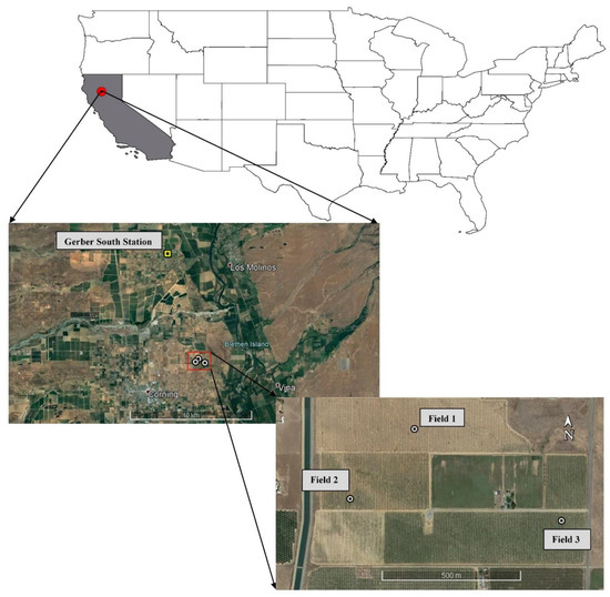
Figure 1.
The study area. The white dots are representative of EC towers, the red polygon is Scheme 2. Ten-year daily average grass reference evapotranspiration (ETr) variations (from 2011 until 2020).
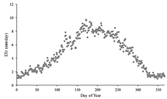
Figure 2.
Ten-year daily average grass reference evapotranspiration (ETr) variations (from 2011 until 2020).
2.2. Datasets
2.2.1. Field Data
Three similar Eddy Covariance (EC) towers were installed in each almond field (Figure 1) located at 39°57′8.7′′N and 122°7′49.2′′W (Field 1), 39°57′0.5′′N and 122°7′59′′W (Field 2), and 39° 56′57.9′′N and 122° 7′26.8′′W (Field 3). Each ET flux tower consisted of: a three-dimensional, sonic anemometer (Model 81000 VRE, R.M. Young Company, Traverse City, MI, USA) oriented in the prevailing wind direction; a net radiometer (NR-LITE, Campbell Scientific, Logan, UT, USA); and soil heat flux plates at 5 cm depth (HFT3.1, REBS, Bellevue, WA, USA). Auxiliary data include air temperature and relative humidity, soil water content, and soil thermocouples at 5 cm depth, and a tipping rain gauge. Each orchard had enough fetch to accurately estimate ET using each flux tower. Sensible heat flux (H) was quantified using the eddy covariance method from data collected using a 3D sonic anemometer and fine-wire thermocouples at a sampling frequency of 10 Hz. Soil heat flux (G) was measured using three soil heat flux plates and soil thermocouples, and adjusted for moisture content using three capacitance sensors (ECH2O EC5) on the top 5 cm depth. ETa was calculated as the residual of the energy balance equation (λET = Rn − G − H) and averaged over 30 min.
The flux footprint of the towers were predicted based on Kljun et al. [42] using the online data processing (http://footprint.kljun.net/, accessed on 5 June 2021). Accordingly, pixels within the footprint area were used to optimally compare the EC data against remotely sensed ETa.
2.2.2. Remotely Sensed Data
Satellite: Four Landsat 8 surface reflectance products were pre-processed in Google Earth Engine (Table 1). Cloud cover and water bodies were removed using the quality band provided for the surface reflectance product. Landsat 8 contains 11 bands, 7 of which are commonly used for agricultural purposes (Table 2) and cover visible (VIS), near infrared (NIR), and SWIR portions. An area was clipped from the images so that it mostly represented agricultural fields and was big enough to contain more than 60,000 pixels for extracting the LST-VI relationship, while also being small enough not to capture heights where temperature drops drastically. Image processing was conducted using MATLAB.

Table 1.
Date of data collection.
Table 2.
Landsat 8 (OLI/TIRS) and UAV (Micasense Altum) band specifications.
UAV: Three flights (Table 1) were conducted over the three almond fields using a quadcopter (DJI Matrice 210) equipped with a high resolution multispectral and thermal sensor (Micasense Altum) and an RGB camera (Zenmus X4S). Raw images were pre-processed in Agisoft Metashape software. The images were ortho-rectified and layerstacked to achieve single TIFF files containing Blue, Green, Red, Red-edge, Infra-Red and thermal bands (Table 2). Subsequently, further processes were done in ENVI 5.3.
Comparison: Landsat 8 and UAV images covered almost the same portions over VIS/NIR, with small differences in bandwidths. Their spatial resolution differed significantly, with 30 m fixed for Landsat 8 compared to 2.65 and 3.23 cm for UAV, depending on flight altitude (Table 3). To achieve an orthomosaic of good quality, images were captured with 90% overlap. A calibrated reflectance panel was used before and after each flight to convert raw pixel values into reflectance. UAV images were acquired between 11:00 AM and 1:30 P.M (Table 3) to reduce the shading effect and to match as much as possible LandSat passage (around 11:38 am in local time).
Table 3.
Acquisition time in Pacific Standard Time (PST), flight height above ground level and spatial resolution of the UAV campaigns at the three almond sites.
2.2.3. Meteorological Data
The California Department of Water Resources (DWR) manages over 145 automated weather station in California under the California Irrigation Management Information System (CIMIS) program. CIMIS is a joint program between DWR and the University of California, Davis, assisting researchers utilize meteorological data to precisely manage California’s water resources and crop water use.
The meteorological data used in the algorithms were obtained from the Gerber South station (Station id: 222) situated at 40°1′48′′N and 122°9′36′′N, comprising solar radiation (Rs), vapor pressure, air temperature (Ta), relative humidity, dew point, and wind speed. The hourly data were obtained specifically for the date of Landsat 8 overpasses and UAV flights and 10 years of daily data for ET0 calculation.
The five-year annual precipitation was 416.1 mm; however, 2019, where two of our flights were conducted, was a wet year with 650.9 mm precipitation. The 2019–2020 time series of daily precipitation is shown in Figure 3.
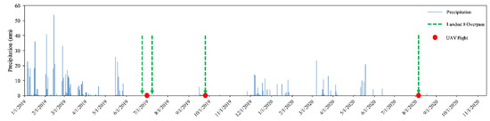
Figure 3.
Daily precipitation of Gerber South station during 2019–2020.
2.3. Mapping EvapoTranspiration at High Resolution with Internalized Calibration (METRIC)
The METRIC model was developed by Allen et al. [8] and validated in Allen et al. [9]. METRIC has proven to demonstrate promising accuracy calculating Landsat [43,44,45,46,47] and UAV [10,46] images. For this reason ETa from remotely sensed data were chosen to be calculated using this model in this study.
The ETa calculation process was almost the same for both Landsat 8 and UAV images, with the slight differences pointed out during the model description in the current section. Both sets of data required hot and cold pixel identification in order to establish a relationship between LST and the difference between Ta and LST (dT0 for iteratively finding the corresponding coefficients, “a” and “b” (dT = aLST + b) by considering the stability conditions of the atmosphere. The energy required for ETa (λET) was obtained as the residual of the energy balance equation:
where Rn was calculated by determining the shortwave and longwave radiation intercepting the ground and reflected and emitted from the ground:
where Rs is the incoming shortwave radiation assuming clear sky conditions; RL↓ and RL↑ are the incoming and outgoing longwave radiations, respectively, as the function of air temperature and LST to the fourth power (the Stefan–Boltzman law); ε0 is the surface emissivity, described in terms of vegetation cover; and α is the surface albedo, which had different calculation procedures for satellite (Equation (3) [48]) and UAV (Equation (4) [49]) images:
where Ꞷb is the weight of each band in the Landsat 8 spectral range; ρb is the reflectance of each band; VIS is the reflectance corresponding to the visible bands, and NIR is the reflectance of the Near Infrared band of the UAV. An NDVI greater equal than 0.25 was considered vegetation and lower than 0.25 bare soil.
λET = Rn − G − H
Rn = (1 − α)Rs + RL↓ − RL↑ − (1 − ε0) RL↓
G was calculated based on the empirical formulation presented in [50]:
H was iteratively identified using the stability conditions of the pixels under both Landsat 8 and UAV conditions. The heat gradient was determined by the heat transfer formula of Newton’s law divided by the aerodynamic resistance (rah).
where ρa is the air density; Cp is the specific heat of vaporization; rah s the aerodynamic resistance; K is the Von Karman’s constant (0.41); u* is the friction velocity; z is the reference height (2 m above the ground); zoh is the roughness length for heat flux (0.1 m); ψm and ψh are the stability corrections for momentum and heat transport, respectively; u200 is the wind speed at a height where the surface does not affect the wind function (200 m above the ground); and z0m is the roughness length for momentum flux.
The Equation (1) output was instantaneous λET (W·m−2) converted to ETa,inst (mm·h−1). Hence, in order to achieve daily ETa (ETa,daily (mm·day−1)), the following approach was taken:
where ETr,inst and ETr,daily are the hourly and daily reference evapotranspiration, respectively, calculated from the FAO Penman-Monteith equation [51], and ETrf is the reference ET fraction.
2.4. Modified TsHARP Method: The Multi-Sensor Data Fusion Model for Actual Evapotranspiration Estimation (MSDF-ET)
The TsHARP method was originally developed to sharpen the MODIS LST products to the Landsat resolution based on the relationship between LST and VIs [21]. This has proven to be a reliable method for downscaling thermal information [52], focusing on sharpening the instantaneous LST; however, [53] pioneered the use of daytime and nighttime LST of the MODIS onboard both Terra and Aqua for downscaling the 24-h LST to the Landsat resolution in order to calculate potential ET. In this study, the same concept was adapted to directly enhance the resolution of Landsat 8-based ETa to acquire very high resolution maps of crop water use.
One of the prominent factors affecting the magnitude of ETa is, undeniably, the density of vegetation covering the ground. Therefore, it is presumed that a strong linear relationship exists between ETa and VIs calculated from the VIS-IR bands of Landsat 8. However, considering that it would not always be possible to acquire UAV images coinciding with the Landsat 8 overpass, and ETa is not transferable from one day to another, ETrf was employed for linear interpolation between two consecutive Landsat 8 overpasses to acquire an image coinciding with the UAV flight [54]. Since ETrf gives specific information of each pixel, and relative changes in weather are identified from ETr (and ETa changes proportionally to ETr [54]), this approach was taken into account for ETa interpolation in order to achieve its monthly variations [43].
The MSDF-ET method consisted of the following steps (Figure 4):
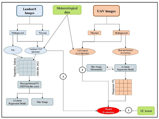
Figure 4.
The summary of the MSDF-ET method to calculate ETa.
- Different VIs (Table 4) were calculated from different bands of Landsat 8 including NDVI, SAVI, EVI, NDWI, and LSWI. The reason for selecting these VIs was mainly due to the emanations from the different bands used in their formulation (Blue, Red, NIR, SWIR1, and SWIR2), as well as the soil correction coefficient used in SAVI, because the study area was an orchard exposing a high soil surface area, and atmospheric correction in EVI.
Table 4. Vegetation indices formulations.
- To find the most suitable VI for the method, the ETrf-VI relationships were investigated before proceeding with the MSDF-ET application on ETrf estimation.
- The most suitable VI was selected and a linear relationship was established for each Landsat 8 overpass to find the slope (a) and intercept of the equation (b):where ETrfLC08 is the ETrf calculated from the METRIC algorithm using the Landsat 8 multispectral/thermal bands, and VILC08 is the most suitable VI calculated from Landsat 8 multispectral bands.
- Once “a” and “b” were found, a Bias image for each overpass was constructed to suppress the effects of non-vegetation phenomena on the ETrf variations:where ETrfLC08,unc is the uncorrected ETrf calculated from “a” and “b”, which were obtained from step 3 (Equation (11)) and Bias is the image containing the effects of non-vegetation objects covering the ground.
- Having calculated the Bias image, an uncorrected ETrf was calculated using the multispectral bands of the UAV images (ETrfUAV,unc):
- In the end, the Bias image was resampled and applied to ETrfUAV,unc to achieve the true ETrf of the UAV images without the help of UAV-based thermal bands:ETrfUAV, MSDF-ET = Bias + ETrfUAV,unc
2.5. Model Evaluation
The model was evaluated in four steps:
- Directly evaluating the results with the ETa measured using the three EC towers installed in the almond fields.
- A pixel-by-pixel evaluation of the model against ETa calculated from the METRIC model using the UAV images.
- A pixel-by-pixel evaluation of the model against ETa calculated from the METRIC model using the Landsat 8 images.
- Visual interpretation of the ETa maps.
2.6. Statistical Analysis
The statistical parameters consisted of the coefficient of determination (R2) showing the correlation between parameters and the Root Mean Squared Error (RMSE) indicative of the dispersion of the points from the 1:1 line.
where RSS is the sum of squares of residuals, TSS is the total sum of squares, Pj is the predicted value, Oj is the observed value and n is the number of data.
3. Results
3.1. METRIC-Based ETa
3.1.1. Against the Measured Data
METRIC was applied to both satellite and UAV (multispectral/thermal) images. The results were evaluated against EC data (Figure 5). In this section, we made an effort to discuss the reasons behind the errors that occurred in both UAV and Landsat 8 results. The differences in R2 values were not significant (R2 = 0.74 for Landsat 8 and R2 = 0.77 for UAV images); however, the dispersion of the points from the 1:1 line in UAV images were greater than the Landsat 8 results (RMSE = 1.23 mm/day for UAV against RMSE = 0.81 mm/day for Landsat 8). Mean error (ME) for the Landsat 8 and UAV ETrf were −0.36 and −0.97, respectively, which is indicative of a more severe underestimation in the UAV results. Generally, the underestimation in UAV-based ETa METRIC may have mainly resulted from the lack of a well-watered cold pixel in the UAV’s field of view. By choosing a cold pixel being under conditions, we were in fact considering the maximum ETa at a rate lower than its true value; therefore, ETa, which is linearly changing between 0 and maximum ETa, was subsequently underestimated, which was the reason for the higher RMSE value in the UAV results. Hence, Landsat 8 results showed a lower error compared with the UAV. The Landsat 8 data point distribution in the scatter plot was rooted in several sources such as: bigger coverage of the Landsat 8 pixels in terms of the EC tower coverage, atmospheric correction not being 100 percent precise, a small error in the geometric correction of the images, among others. Since the UAV images were more accurate regarding the capture of surface reflectance and spatial accuracy, the points were more in correlation with the trend line. However, two points (highlighted by a red rectangle in Figure 5) diverged from the other data. These points were those in Field 3 (3rd leaf), with the highest ground cover fraction, where shadows covered the ground considerably. Since the UAV-based ETa METRIC was calculated after removing the shadows over bare soil, the ground cover fraction in this field increased; therefore, it caused ETa to rise more than expected. The shadow effects were only significant on 24 September 2019, and 9 August 2020, which is why ETa on the 1 July 2019 was not influenced by the shadow removal procedure.
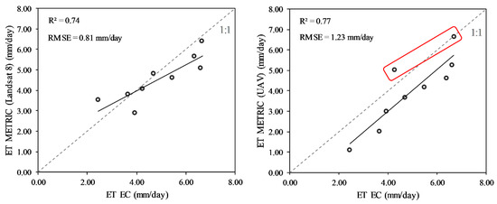
Figure 5.
METRIC-based ETa calculated from Landsat 8 and UAV images against measured ETa.
3.1.2. Correlation with the VIs
Before jumping straight to ETa calculation, the relationship between ETrf and each VI were comprehensively discussed. Four Landsat 8 overpass dates used in this study (Table 1) were considered in the evaluation process (Figure 6). The water bodies were removed from the images, hence the oversaturated points (red elliptical figures) were those pixels that captured irrigated areas, as well as a few ponding surfaces such as pools and swamps. Precipitation in the first half of 2019 was considerably higher than the five-year average (569.5 mm (Figure 3) against 257 mm), which was logically accounted for by the greater amount of moisture content stored in the soil; therefore, this may have been one of the reasons for an increase in ETrf in 2019 and in particular on the 27 June 2019.
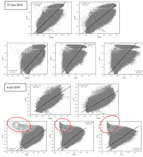
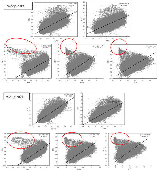
Figure 6.
The ETrf-VI relationships corresponding to the Landsat 8 overpasses.
Outliers caused by oversaturated bare soil pixels (red figures), which accounted for evaporation rather than transpiration, were observed in the VIs computed from the Red and NIR bands, including NDVI, SAVI, and EVI. Such indices have shown to be better correlated with crop transpiration compared with evaporation from the soil, but needless to say that separating transpiration from evaporation from ETrf would not be feasible over a regional scale. Also, the negative values of ETrf commonly occurred under water-stressed bare soil conditions where H was overestimated. These pixels were converted to 0, indicating very low evaporation from the soil. On the other hand, in optical remote sensing, the shortwave infrared (SWIR) portion of the spectrum is the most sensitive to moisture changes in the surface [55], which is why LSWI and NDWI showed more promising correlation against ETrf variability. While oversaturated pixels possessed ETrf > 0.7, they had low values of NDVI, SAVI, and EVI; however, NDWI and LSWI remained high in values over such pixels. Therefore, R2 in the ETrf-NDWI and ETrf-LSWI relationship was frequently higher than ETrf-NDVI, ETrf-SAVI, and ETrf-EVI in all the Landsat 8 overpasses.
Nevertheless, sensors onboard UAVs commonly lack the ability to capture the SWIR portion of the spectrum, and Micasense Altum was not exceptional. Hence, it would not be possible to benefit from the ETrf-NDWI and ETrf-LSWI relationship under the circumstances of this study; however, the next best VI was NDVI, showing a linear relationship with the average R2 of 0.72. Cihlar et al. [31] found an R2 of about 0.6 between ETa and NDVI. In this study, due to the better correlation, NDVI was selected for further calculations. All in all, UAVs containing SWIR bands are recommended for determining water indices such as NDWI and LSWI.
3.2. MSDF-ET Evaluation
3.2.1. Against Measured ETa
ETa calculated using the MSDF-ET method against EC data was investigated and the results were promising (Figure 7). R2 was not higher than the METRIC method (0.68 against 0.77); however, the ETa variability was strongly aligned with the measured data. RMSE was slightly lower than the METRIC-based ETa, representative of the lesser dispersion of the points. Generally, the results showed that the method can be relied upon.
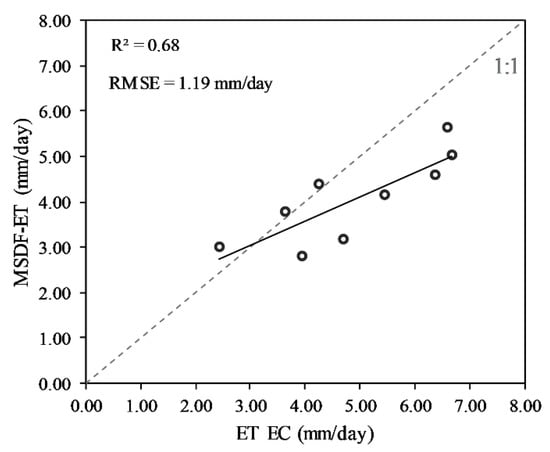
Figure 7.
MSDF-ET ETa against measured ETa.
3.2.2. Against UAV METRIC ETa
The MSDF-ET method was also evaluated against the METRIC algorithm obtained using UAV thermal/multispectral images. ETrf of 9 August 2020 are illustrated as sample correlations over the three fields of almond (Figure 8). First, ETrf from the MSDF-ET was upscaled, then each pixel was evaluated against its corresponding pixel in the METRIC-based ETrf image. The correlations were relatively strong (R2 of 0.62, 0.65, and 0.67 for Field 1, 2, and 3, respectively) with promising RMSE values (0.14, 0.13, and 0.15 for Field 1, 2, and 3, respectively).
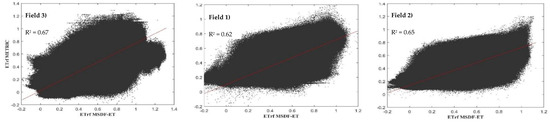
Figure 8.
MSDF-ET ETrf against UAV-based METRIC ETrf.
4. Discussion
4.1. UAV- and Landsat 8-Based NDVI Comparison
NDVI calculated from UAV and Landsat 8 were both averaged over each field. First, the noData pixels on the edges were removed and an inside area of interest was chosen to clip the images. Then, a simple aerial average of the NDVI was computed for both UAV and Landsat 8 and d against each other (Figure 9). UAV and Landsat had very similar NDVIs except for the 24th of September 2019 at Field 2 and Field 3. This discrepancy resulted from the fact that the irrigation system was running on both fields, making the wetting patterns clearly visible, especially on young orchards where most of the ground is exposed. Another reason is related to the extended shadowed area on both orchards created by the slight difference between UAV flights and Landsat overpass time (11:40 PST) (Table 3). In the ETa evaluation from MSDF-ET (Figure 7), the differences were suppressed using the Bias image (Step 4 equation 13). Generally, further studies need to be conducted to investigate the precise sources of discrepancies in UAV and Landsat 8 vegetation indices, especially on partly covered fields.
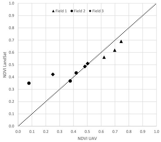
Figure 9.
Comparison between NDVI calculated from UAV and Landsat 8 images.
4.2. Differences in Spatial Resolution (UAV vs. Landsat 8)
An increase in pixel size limited to less than twice the smallest row spacing over an orchard does not affect ETa accuracy [3]; however, it may impede its use for precision agriculture, such as detecting diseases on a single tree, irrigation system malfunctioning, over-irrigation or water stress at a microscale, ponding locations, and so on. Figure 6 shows the difference in Landsat 8 and UAV spatial resolution on the 1st of July 2019 corresponding to the Field 1, where shadow was at its lowest. In the UAV image (Figure 10a), each tree could be precisely visualized, and the well-grown trees were easily distinguishable. On the other hand, the Landsat 8 orchard illustration (Figure 10b) where all the pixels were mixed, containing different ground covers, was only limited to an estimation of well-grown and -watered areas, with the size of 30 × 30 m2. Also, the range of ETa was lower over the field in the Landsat 8 image compared with the UAV due to the mixture of objects (soil and vegetation) in each pixel.
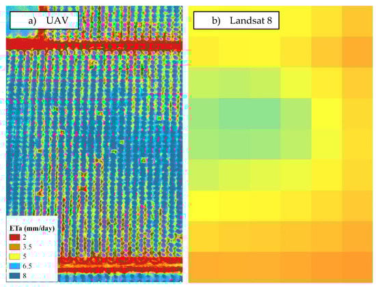
Figure 10.
Illustration of the difference between (a) UAV and (b) Landsat spatial resolutions over Field 1 on 1 July 2019.
4.3. Visual Interpretation (MSDF-ET vs. METRIC UAV)
By visually analyzing the output ETa from both METRIC and MSDF-ET methods (Figure 11), it was recognized that the model could properly distinguish the spatial differences in ETa and was suitable for ETa mapping over the almond orchard. Due to higher spatial resolution of the MSDF-ET method, the field was mapped with more details. The canopy covers and the spaces between rows and trees were more distinguishable. Even the ETa over a single tree showed more details.
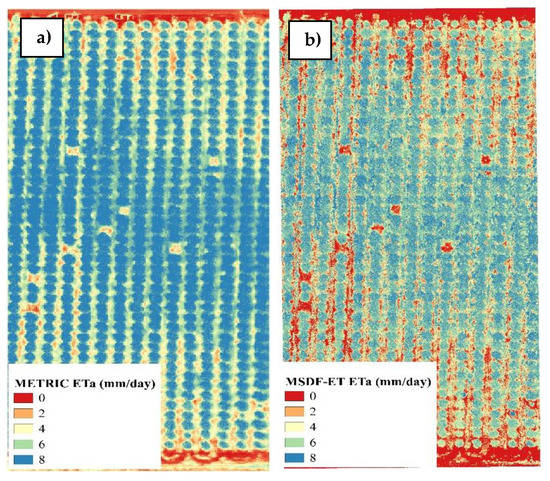
Figure 11.
ETa maps obtained using (a) METRIC and (b) MSDF-ET methods over Field 3 on the 1 July 2019.
4.4. Soil Moisture Detection (MSDF-ET vs. METRIC UAV)
The performance of the MSDF-ET and METRIC methods were visually investigated for detecting soil moisture and subsequently irrigated areas over soil at the UAV scale (Figure 12). The UAV flight over Field 2 on 1 July 2019 was captured during an irrigation event. The northern part of the field received excessive water that caused runoff causing extra water discharged to the road between the fields (red rectangle in Figure 12a). Irrigated water can be clearly distinguished in the true color image, and the METRIC method also presented significantly higher values of ETrf over the saturated soil (light blue pixels in the METRIC image, Figure 12b). However, the MSDF-ET method was not able to properly detect the wetted soil (Figure 12c), which was a disadvantage to this method. Also, both approaches were successful in distinguishing the weeds between rows, but with more details in the MSDF-ET image due to higher spatial resolution.
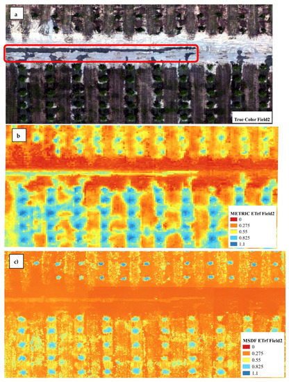
Figure 12.
(a) True Color, (b) METRIC- and (c) MSDF-ET-based ETrf over an excessive irrigated area in Field 2, on 1 July 2019. The red rectangle in the true color image highlights leakage water from the irrigation system.
4.5. Shadow Effects (MSDF-ET vs. METRIC UAV)
Shadows may cause bias in ETa obtained from high spatial resolution imagery [56]. The UAV flight on 24 September 2019 was captured in the afternoon, which caused several shadowy pixels over the three fields. The Field 2 true color (Figure 13a), NDVI (Figure 13b), ETa from MSDF-ET (Figure 13c), LST (Figure 13d), and ETa from METRIC (Figure 13e) images are shown as samples of which shadows were visually distinguished. The pixels superimposed over shadows resulted in lesser values of LST. The lower the LST, the weaker the longwave radiation emitted from the ground based on the Stefan–Boltzman law. Therefore, the Rn and subsequently ETa of the shadowy pixels (blue pixels in Figure 13e) rose above the ETa compared with the pixels over vegetation, which was unusual. In these cases, we were obliged to remove the shadows in order to calculate ETa with better reliability, which still inevitably forced biases, however small, in the ETa maps. However, NDVI was only slightly affected by shadow, so subsequent MSDF-ET-based ETa was calculated even over shadowy pixels. Zhang et al. [57] tested the effects of shadow on different vegetation indices calculated using a hyperspectral spectroradiometer and found that NDVI was the least affected index. Therefore, the use of NDVI in the MSDF-ET method was beneficial for attenuating the effects of shadow on ETa calculation.
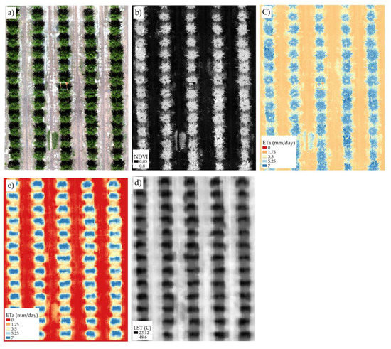
Figure 13.
(a) true color, (b) NDVI, (c) MSDF-ET ETa, (d) LST, and (e) METRIC ETa images over Field 2.
4.6. Advantages and Disadvantages of the MSDF-ET Method
Advantages:
- The foremost advantage was the higher spatial resolution of the resulting ETa maps.
- The thermal image was excluded, which may result in a less expensive device for ETa mapping.
- Albedo calculation procedure using UAV images was removed, as these images usually suffer from the lack of bands covering the shortwave infrared portion of the spectrum, inevitably causing errors in ETa maps.
- Finding a well-watered vegetation or a fully dry surface in the limited UAV’s field of view has been always challenging, and the MSDF-ET method removed the need for hot and cold pixel selection.
- Due to METRIC-based ETa calculations applied to Landsat 8 images, the process was not heavy and could be executed on a low-performance laptop.
- Instead of sharpening LST to the UAV resolution, which was not transferable from one date to another, ETrf was used to omit this limitation and apply the MSDF-ET method to UAV images not captured in the Landsat 8 overpasses.
Disadvantages:
- The wet soils could not be clearly distinguished compared with the METRIC method.
- In cases of cloudy Landsat images, the interval between two consecutive Landsat overpasses is increased, and subsequently the accuracy decreases (however the launch of Landsat 9 would immensely reduce the risk).
5. Conclusions
This study focused on a new method for calculating ETa from UAV multispectral images without the use of thermal information from the surface. The method was a modified version of the TsHARP algorithm, which sharpens the MODIS LST product to Landsat resolution; however, Landsat 8-based ETrf was sharpened instead of LST in order to make the method feasible for achieving ETa maps of flights captured in between Landsat overpasses. The method in this study was referred to as MSDF-ET. The statistical and visual evaluation of the method showed promising results. The correlation between MSDF-ET ETa against EC data collected over three almond fields was reliable, with an R2 of 0.68 and RMSE of 1.19 mm/day. Further evaluations against UAV- and Landsat 8-derived ETa showed slightly lower correlations, with the error partly resulting from upscaling the pixels. The visual interpretation was indicative of the proper performance of the method. In the MSDF-ET method, ETa over trees was shown in detail and shadows had negligible effects on ETa values, while on the other hand ETa using a UAV derived from the METRIC algorithm was significantly affected by the shadows. The lower sensitivity of the MSDF-ET method to shadows resulted from the slight effects of shadow on the NDVI. By using this method, the need for a thermal camera onboard a UAV was reduced. UAV images do not usually capture well-watered vegetation or fully dried surfaces due to the limited area for image capturing; however, the MSDF-ET method eliminated the hot/cold pixel selection procedure of UAV images. Also, UAVs commonly suffer from a lack of shortwave infrared cameras for Albedo calculation, which was also removed in the MSDF-ET method. Needless to say, the resulting ETa maps from multispectral images possessed higher spatial resolutions compared to the ETa maps from LST images (METRIC algorithm). In general, the methods such the one presented in this study focusing on ETa mapping using only multispectral images may significantly reduce operational and investment costs due to removing the need for thermal cameras.
Author Contributions
Conceptualization, A.M., A.A. and A.D.; methodology, A.M., A.A. and A.D.; software, A.M., A.A., A.D. and K.D.; validation, A.M., A.D. and K.D.; formal analysis, A.M. and A.A.; resources, A.D. and K.D.; data curation, A.M, A.A., K.D. and A.D.; writing—original draft preparation, A.M and A.A.; writing—review and editing, A.D.; visualization, A.M., A.A., A.D and K.D.; supervision, A.D.; project administration, A.D. All authors have read and agreed to the published version of the manuscript.
Funding
This research received no external funding.
Conflicts of Interest
The authors declare no conflict of interest.
References
- Roser, M.; Hannah Ritchie, H.; Esteban Ortiz-Ospina, E. World Population Growth. Published online at OurWorldInData.org. 2013. Available online: https://ourworldindata.org/world-population-growth (accessed on 12 June 2021).
- FAO. Crops and Drops: Making the Best Use of Water for Agriculture; Food and Agriculture Organization of the United Nations: Rome, Italy, 2000.
- Nassar, A.; Torres-Rua, A.; Kustas, W.; Nieto, H.; McKee, M.; Hipps, L.; Stevens, D.; Alfieri, J.; Prueger, J.; Alsina, M.M.; et al. Influence of Model Grid Size on the Estimation of Surface Fluxes Using the Two Source Energy Balance Model and sUAS Imagery in Vineyards. Remote Sens. 2020, 12, 342. [Google Scholar] [CrossRef] [PubMed]
- Wang, T.; Tang, R.; Li, Z.-L.; Jiang, Y.; Liu, M.; Niu, L. An Improved Spatio-Temporal Adaptive Data Fusion Algorithm for Evapotranspiration Mapping. Remote Sens. 2019, 11, 761. [Google Scholar] [CrossRef]
- McCabe, M.F.; Rodell, M.; Alsdorf, D.E.; Miralles, D.G.; Uijlenhoet, R.; Wagner, W.; Lucieer, A.; Houborg, R.; Verhoest, N.E.C.; Franz, T.E.; et al. The future of Earth observation in hydrology. Hydrol. Earth Syst. Sci. 2017, 21, 3879–3914. [Google Scholar] [CrossRef]
- Bastiaanssen, W.; Menenti, M.; Feddes, R.; Holtslag, A. A remote sensing surface energy balance algorithm for land (SEBAL). Formulation. J. Hydrol. 1998, 212, 198–212. [Google Scholar] [CrossRef]
- Su, Z. The Surface Energy Balance System (SEBS) for estimation of turbulent heat fluxes. Hydrol. Earth Syst. Sci. 2002, 6, 85–100. [Google Scholar] [CrossRef]
- Allen, R.G.; Tasumi, M.; Trezza, R. Satellite-Based Energy Balance for Mapping Evapotranspiration with Internalized Calibration (METRIC)—Model. J. Irrig. Drain. Eng. 2007, 133, 380–394. [Google Scholar] [CrossRef]
- Allen, R.G.; Tasumi, M.; Morse, A.; Trezza, R.; Wright, J.L.; Bastiaanssen, W.; Kramber, W.; Lorite, I.; Robison, C.W. Satellite-Based Energy Balance for Mapping Evapotranspiration with Internalized Calibration (METRIC)—Applications. J. Irrig. Drain. Eng. 2007, 133, 395–406. [Google Scholar] [CrossRef]
- Ramírez-Cuesta, J.; Allen, R.; Zarco-Tejada, P.; Kilic, A.; Santos, C.; Lorite, I. Impact of the spatial resolution on the energy balance components on an open-canopy olive orchard. Int. J. Appl. Earth Obs. Geoinform. 2019, 74, 88–102. [Google Scholar] [CrossRef]
- Norman, J.; Kustas, W.; Humes, K. Source approach for estimating soil and vegetation energy fluxes in observations of directional radiometric surface temperature. Agric. For. Meteorol. 1995, 77, 263–293. [Google Scholar] [CrossRef]
- Xia, T.; Kustas, W.P.; Anderson, M.C.; Alfieri, J.G.; Gao, F.; McKee, L.; Prueger, J.H.; Geli, H.M.E.; Neale, C.M.U.; Sanchez, L.; et al. Mapping evapotranspiration with high-resolution aircraft imagery over vineyards using one- and two-source modeling schemes. Hydrol. Earth Syst. Sci. 2016, 20, 1523–1545. [Google Scholar] [CrossRef]
- Cheng, J.; Kustas, W.P. Using Very High Resolution Thermal Infrared Imagery for More Accurate Determination of the Impact of Land Cover Differences on Evapotranspiration in an Irrigated Agricultural Area. Remote Sens. 2019, 11, 613. [Google Scholar] [CrossRef]
- Torres-Rua, A.; Ticlavilca, A.M.; Aboutalebi, M.; Nieto, H.; Alsina, M.M.; White, A.; Prueger, J.H.; Alfieri, J.; Hipps, L.; McKee, L.; et al. Estimation of evapotranspiration and energy fluxes using a deep learning-based high-resolution emissivity model and the two-source energy balance model with sUAS information. In Proceedings of the Autonomous Air and Ground Sensing Systems for Agricultural Optimization and Phenotyping, International Society for Optics and Photonics, Bellingham, DC, USA, 14 May 2020; Volume 11414, p. 114140B. [Google Scholar]
- Aboutalebi, M.; Torres-Rua, A.F.; McKee, M.; Kustas, W.P.; Nieto, H.; Alsina, M.M.; White, A.; Prueger, J.H.; McKee, L.; Alfieri, J.; et al. Incorporation of Unmanned Aerial Vehicle (UAV) Point Cloud Products into Remote Sensing Evapotranspiration Models. Remote Sens. 2020, 12, 50. [Google Scholar] [CrossRef]
- Zipper, S.C.; Loheide, S.P. Using evapotranspiration to assess drought sensitivity on a subfield scale with HRMET, a high resolution surface energy balance model. Agric. For. Meteorol. 2014, 197, 91–102. [Google Scholar] [CrossRef]
- Castelli, M.; Asam, S.; Jacob, A.; Zebisch, M.; Notarnicola, C. Monitoring daily evapotranspiration in the Alps ex-ploiting Sentinel-2 and meteorological data. In Proceedings of the Remote Sensing and Hydrology Symposium (ICRS-IAHS), Cordoba, Spain, 8–10 May 2018. [Google Scholar]
- Rozenstein, O.; Haymann, N.; Kaplan, G.; Tanny, J. Estimating cotton water consumption using a time series of Sentinel-2 imagery. Agric. Water Manag. 2018, 207, 44–52. [Google Scholar] [CrossRef]
- Vanino, S.; Nino, P.; De Michele, C.; Bolognesi, S.F.; D’Urso, G.; Di Bene, C.; Pennelli, B.; Vuolo, F.; Farina, R.; Pulighe, G.; et al. Capability of Sentinel-2 data for estimating maximum evapotranspiration and irrigation requirements for tomato crop in Central Italy. Remote Sens. Environ. 2018, 215, 452–470. [Google Scholar] [CrossRef]
- Teixeira, A.H.D.C. Determining Regional Actual Evapotranspiration of Irrigated Crops and Natural Vegetation in the São Francisco River Basin (Brazil) Using Remote Sensing and Penman-Monteith Equation. Remote Sens. 2010, 2, 1287–1319. [Google Scholar] [CrossRef]
- Agam, N.; Kustas, W.P.; Anderson, M.C.; Li, F.; Neale, C.M. A vegetation index based technique for spatial sharpening of thermal imagery. Remote Sens. Environ. 2007, 107, 545–558. [Google Scholar] [CrossRef]
- Weng, Q.; Fu, P.; Gao, F. Generating daily land surface temperature at Landsat resolution by fusing Landsat and MODIS data. Remote Sens. Environ. 2014, 145, 55–67. [Google Scholar] [CrossRef]
- Lillo-Saavedra, M.; García-Pedrero, A.; Merino, G.; Gonzalo-Martín, C. TS2uRF: A New Method for Sharpening Thermal Infrared Satellite Imagery. Remote Sens. 2018, 10, 249. [Google Scholar] [CrossRef]
- Cammalleri, C.; Anderson, M.C.; Gao, F.; Hain, C.R.; Kustas, W.P. A data fusion approach for mapping daily evapotranspiration at field scale. Water Resour. Res. 2013, 49, 4672–4686. [Google Scholar] [CrossRef]
- Knipper, K.R.; Kustas, W.P.; Anderson, M.C.; Alfieri, J.G.; Prueger, J.H.; Hain, C.R.; Hipps, L.E. Evapotran-spiration estimates derived using thermal-based satellite remote sensing and data fusion for irrigation management in California vineyards. Irrig. Sci. 2019, 37, 431–449. [Google Scholar] [CrossRef]
- Mokhtari, A.; Noory, H.; Pourshakouri, F.; Haghighatmehr, P.; Afrasiabian, Y.; Razavi, M.; Naeni, A.S. Calcu-lating potential evapotranspiration and single crop coefficient based on energy balance equation using Landsat 8 and Senti-nel-ISPRS. J. Photogramm. Remote Sens. 2019, 154, 231–245. [Google Scholar] [CrossRef]
- Mokhtari, A.; Noory, H.; Vazifedoust, M.; Palouj, M.; Bakhtiari, A.; Barikani, E.; Afrooz, R.A.Z.; Fereydooni, F.; Naeni, A.S.; Pourshakouri, F.; et al. Evaluation of single crop coefficient curves derived from Landsat satellite images for major crops in Iran. Agric. Water Manag. 2019, 218, 234–249. [Google Scholar] [CrossRef]
- Xue, J.; Anderson, M.C.; Gao, F.; Hain, C.; Sun, L.; Yang, Y.; Knipper, K.R.; Kustas, W.P.; Torres-Rua, A.; Schull, M. Sharpening ECOSTRESS and VIIRS land surface temperature using harmonized Landsat-Sentinel surface reflectances. Remote Sens. Environ. 2020, 251, 112055. [Google Scholar] [CrossRef] [PubMed]
- Guzinski, R.; Nieto, H. Evaluating the feasibility of using Sentinel-2 and Sentinel-3 satellites for high-resolution evapotranspiration estimations. Remote Sens. Environ. 2019, 221, 157–172. [Google Scholar] [CrossRef]
- Guzinski, R.; Nieto, H.; Sandholt, I.; Karamitilios, G. Modelling High-Resolution Actual Evapotranspiration through Sentinel-2 and Sentinel-3 Data Fusion. Remote Sens. 2020, 12, 1433. [Google Scholar] [CrossRef]
- Cihlar, J.; St.-Laurent, L.; Dyer, J. Relation between the normalized difference vegetation index and ecological variables. Remote Sens. Environ. 1991, 35, 279–298. [Google Scholar] [CrossRef]
- Choudhury, B.; Ahmed, N.; Idso, S.; Reginato, R.; Daughtry, C. Relations between evaporation coefficients and vegetation indices studied by model simulations. Remote Sens. Environ. 1994, 50, 1–17. [Google Scholar] [CrossRef]
- Mateos, L.; González-Dugo, M.; Testi, L.; Villalobos, F. Monitoring evapotranspiration of irrigated crops using crop coefficients derived from time series of satellite images. I. Method validation. Agric. Water Manag. 2013, 125, 81–91. [Google Scholar] [CrossRef]
- Dos Santos, R.A.; Mantovani, E.C.; Filgueiras, R.; Fernandes-Filho, E.I.; Da Silva, A.C.B.; Venancio, L.P. Actual Evapotranspiration and Biomass of Maize from a Red–Green-Near-Infrared (RGNIR) Sensor on Board an Unmanned Aerial Vehicle (UAV). Water 2020, 12, 2359. [Google Scholar] [CrossRef]
- Rouse, J.W., Jr.; Haas, R.H.; Deering, D.W.; Schell, J.A.; Harlan, J.C. Monitoring the Vernal Advancement and Retrogradation (Green Wave Effect) of Natural Vegetation; Great Plains Corridor; Texas A&M University: College Station, TX, USA, 1974. [Google Scholar]
- Huete, A. A soil-adjusted vegetation index (SAVI). Remote Sens. Environ. 1988, 25, 295–309. [Google Scholar] [CrossRef]
- Liu, H.Q.; Huete, A. A feedback based modification of the NDVI to minimize canopy background and atmospheric noise. IEEE Trans. Geosci. Remote Sens. 1995, 33, 457–465. [Google Scholar] [CrossRef]
- Nolet, C.; Poortinga, A.; Roosjen, P.; Bartholomeus, H.; Ruessink, G. Measuring and Modeling the Effect of Surface Moisture on the Spectral Reflectance of Coastal Beach Sand. PLoS ONE 2014, 9, e112151. [Google Scholar] [CrossRef]
- Gao, B.-C. NDWI—A normalized difference water index for remote sensing of vegetation liquid water from space. Remote Sens. Environ. 1995, 58, 257–266. [Google Scholar] [CrossRef]
- McFeeters, S.K. The use of the Normalized Difference Water Index (NDWI) in the delineation of open water features. Int. J. Remote Sens. 1996, 17, 1425–1432. [Google Scholar] [CrossRef]
- Abatzoglou, J.T. Development of gridded surface meteorological data for ecological applications and modelling. Int. J. Clim. 2013, 33, 121–131. [Google Scholar] [CrossRef]
- Kljun, N.; Calanca, P.; Rotach, M.W.; Schmid, H.P. A simple two-dimensional parameterisation for Flux Footprint Prediction (FFP). Geosci. Model Dev. 2015, 8, 3695–3713. [Google Scholar] [CrossRef]
- Lian, J.; Huang, M. Comparison of three remote sensing based models to estimate evapotranspiration in an oa-sis-desert region. Agric. Water Manag. 2016, 165, 153–162. [Google Scholar] [CrossRef]
- Bhattarai, N.; Quackenbush, L.J.; Im, J.; Shaw, S.B. A new optimized algorithm for automating endmember pixel selection in the SEBAL and METRIC models. Remote Sens. Environ. 2017, 196, 178–192. [Google Scholar] [CrossRef]
- Wagle, P.; Bhattarai, N.; Gowda, P.H.; Kakani, V.G. Performance of five surface energy balance models for esti-mating daily evapotranspiration in high biomass sorghum. ISPRS J. Photogramm. Remote Sens. 2017, 128, 192–203. [Google Scholar] [CrossRef]
- Jaafar, H.H.; Ahmad, F.A. Time series trends of Landsat-based ET using automated calibration in METRIC and SEBAL: The Bekaa Valley, Lebanon. Remote Sens. Environ. 2020, 238, 111034. [Google Scholar] [CrossRef]
- Chávez, J.L.; Gowda, P.H.; Howell, T.A.; Garcia, L.A.; Copeland, K.S.; Neale, C.M.U. ET Mapping with High-Resolution Airborne Remote Sensing Data in an Advective Semiarid Environment. J. Irrig. Drain. Eng. 2012, 138, 416–423. [Google Scholar] [CrossRef]
- Waters, R.; Allen, R.; Tasumi, M.; Trezza, R.; Bastiaanssen, W.G.M. SEBAL (Surface Energy Balance Algorithms for Land): Advanced Training and User’s Manual; Department of Water Resources, University of Idaho: Kimberly, ID, USA, 2002; p. 98. [Google Scholar]
- Brest, C.L.; Goward, S.N. Deriving surface albedo measurements from narrow band satellite data. Int. J. Remote Sens. 1987, 8, 351–367. [Google Scholar] [CrossRef]
- Bastiaanssen, W. SEBAL-based sensible and latent heat fluxes in the irrigated Gediz Basin, Turkey. J. Hydrol. 2000, 229, 87–100. [Google Scholar] [CrossRef]
- Allen, R.G.; Pereira, L.S.; Raes, D.; Smith, M. Crop evapotranspiration-Guidelines for computing crop water requirements-FAO Irrigation and drainage paper. FAO Rome 1998, 300, D05109. [Google Scholar]
- Huryna, H.; Cohen, Y.; Karnieli, A.; Panov, N.; Kustas, W.P.; Agam, N. Evaluation of TsHARP Utility for Thermal Sharpening of Sentinel-3 Satellite Images Using Sentinel-2 Visual Imagery. Remote Sens. 2019, 11, 2304. [Google Scholar] [CrossRef]
- Mokhtari, A.; Noory, H.; Vazifedoust, M.; Bahrami, M. Estimating net irrigation requirement of winter wheat using model- and satellite-based single and basal crop coefficients. Agric. Water Manag. 2018, 208, 95–106. [Google Scholar] [CrossRef]
- Allen, R.G.; Irmak, A.; Trezza, R.; Hendrickx, J.M.H.; Bastiaanssen, W.G.M.; Kjaersgaard, J. Satellite-based ET estimation in agriculture using SEBAL and METRIC. Hydrol. Process. 2011, 25, 4011–4027. [Google Scholar] [CrossRef]
- Sadeghi, M.; Jones, S.B.; Philpot, W.D. A linear physically-based model for remote sensing of soil moisture using short wave infrared bands. Remote Sens. Environ. 2015, 164, 66–76. [Google Scholar] [CrossRef]
- Aboutalebi, M.; Torres-Rua, A.F.; Kustas, W.P.; Nieto, H.; Coopmans, C.; McKee, M. Assessment of different methods for shadow detection in high-resolution optical imagery and evaluation of shadow impact on calculation of NDVI, and evapotranspiration. Irrig. Sci. 2019, 37, 407–429. [Google Scholar] [CrossRef]
- Zhang, L.; Sun, X.; Wu, T.; Zhang, H. An Analysis of Shadow Effects on Spectral Vegetation Indexes Using a Ground-Based Imaging Spectrometer. IEEE Geosci. Remote Sens. Lett. 2015, 12, 2188–2192. [Google Scholar] [CrossRef]


Publisher’s Note: MDPI stays neutral with regard to jurisdictional claims in published maps and institutional affiliations. |
© 2021 by the authors. Licensee MDPI, Basel, Switzerland. This article is an open access article distributed under the terms and conditions of the Creative Commons Attribution (CC BY) license (https://creativecommons.org/licenses/by/4.0/).