Abstract
Timely and accurate monitoring of tree crop extent and productivities are necessary for informing policy-making and investments. However, except for a very few tree species (e.g., oil palms) with obvious canopy and extensive planting, most small-crown tree crops are understudied in the remote sensing domain. To conduct large-scale small-crown tree mapping, several key questions remain to be answered, such as the choice of satellite imagery with different spatial and temporal resolution and model generalizability. In this study, we use olive trees in Morocco as an example to explore the two abovementioned questions in mapping small-crown orchard trees using 0.5 m DigitalGlobe (DG) and 3 m Planet imagery and deep learning (DL) techniques. Results show that compared to DG imagery whose mean overall accuracy (OA) can reach 0.94 and 0.92 in two climatic regions, Planet imagery has limited capacity to detect olive orchards even with multi-temporal information. The temporal information of Planet only helps when enough spatial features can be captured, e.g., when olives are with large crown sizes (e.g., >3 m) and small tree spacings (e.g., <3 m). Regarding model generalizability, experiments with DG imagery show a decrease in F1 score up to 5% and OA to 4% when transferring models to new regions with distribution shift in the feature space. Findings from this study can serve as a practical reference for many other similar mapping tasks (e.g., nuts and citrus) around the world.
1. Introduction
Producing more food for a growing population and meanwhile reducing poverty, remains two major challenges in many places of the world [1,2,3,4]. Since poor households in developing countries often depend heavily on agriculture for their livelihoods, investing in agricultural productivity has long been used as an important vehicle of pro-poor development [5,6]. Compared to the traditional investment focus of annual staple crops such as cereals, maize, and pulses, recent development programs often favor perennial tree crops for both socio-economic and environmental considerations [7,8,9]. The reasons are multiple. First, tree crops often produce goods with high cash value. Second, investment in tree crops can generate more predictable revenue since a well-maintained orchard may provide stable productions for up to several decades [10]. Third, tree crops often have better adaptability to growth conditions than the annual crops, thus reducing the cost of land clearing [8]. Finally, cultivating tree crops requires fewer management efforts thus allowing farmers to increase incomes through off-farm activities [11]. Examples that tree crops have delivered socioeconomic benefits include but are not limited to coffee in Brazil [12], oil palm in West Africa [13] and Southeast Asia [14], and olives in the Mediterranean [15].
Timely and accurate monitoring of the extent and productivities of tree crops are necessary for enhancing their management [16]. With the increasing accessibility of remote sensing data and the progress in algorithms, there is a surge of studies focusing on mapping different tree crops, e.g., oil palm [17,18,19,20,21,22], rubber [23,24,25], and coffee [26,27,28,29], with multi-source satellite imagery. Despite the varying level of success, these studies mainly fall into two categories. The first group focuses on the identification of individual trees, usually at small scales [30,31,32,33]. Relevant studies largely rely on sophisticatedly designed workflows and independent data sources, e.g., unmanned aerial vehicles (UAV), to finely delineate the shape of individual trees. For example, ref [30] estimated the number, height, diameter, and area of all 117 trees in a pine clonal orchard with UAV images and statistical methods. The second group favors more about mapping the extent and distribution of tree plantation than single tree detection. Studies in this group either feeds hand-crafted spectral, textural, temporal features, and auxiliary data, into traditional classifiers to identify tree crops, or rely on very high resolution (VHR) imagery and more advanced deep learning algorithms such as convolutional neural network (CNN) for automatic feature learning. Typical studies from this group include [24], which applied an ensemble learning approach to map the rubber trees in China based on features including backscatter ratio and difference and time series vegetation indexes extracted from PALSAR and Landsat 5/7 images, respectively, and [18,19], which detected oil palm trees using QuickBird images and two shallow CNN structures, i.e., LeNet [34] and AlexNet [35].
Comparatively, tree species with obvious spatial or spectral features on medium to coarse resolution imagery are much better studied than the small crown trees. For instance, in southeast Asia, mature oil palm trees can have a crown diameter around 10 meters and are often cultivated regularly in plantations that span a few kilometers, thus even coarse-resolution imagery, e.g., MODIS (250 m), can be used to map oil palm plantations [17,22]. In contrast, olive trees in the Mediterranean usually have crown sizes less than 5 m and are more sparsely planted in orchards, therefore are hardly detectable from MODIS imagery or even moderate resolution products like Landsat and Sentinel-2. The same applies to many other fruit trees like almond and citrus. Existing studies for small crown tree crops thus mostly focused on tree counting, statistical relationships, or single crown reconstruction using VHR imagery in a relatively small region (e.g., 90 km2) [36,37,38]. While being useful from the perspective of algorithm development, studies at such a local scale are less relevant to large-scale, policy-oriented applications, such as program evaluation, yield gap analysis, and environmental impact assessment.
Toward mapping tree crops orchards across large regions, several fundamental questions remain to be answered and the two being described below are often of particular concern. First, how effective is high resolution (HR) imagery compared to VHR imagery? Although studies have highlighted the needs for VHR imagery such as the submeter DigitalGlobe (DG) data to detect intra-field tree crop features [39], high acquisition cost and heavy computation loads often prohibit its application to a larger scale. An alternative option is to use multi-temporal HR imagery, such as the PlanetScope constellation that provides near-daily observations of ~3 m yet at a considerably lower price. However, the effectiveness of compensating for the loss of spatial resolution using multi-temporal HR imagery in tree crops mapping remains an open question. Second, how transferable is the classifier trained from one place to another even within the same county (i.e., model generalizability)? This question is less concerning in existing literature when using the medium to coarse resolution imagery partly because it is relatively easy to cover a large area at once. Consequently, the one-time-use model has thus unintentionally reduced the need for transferring. In addition, the widely adopted random sampling protocol for generating training and testing dataset from the same region also helps erase the variation. When it comes to DG-alike VHR imagery, however, the higher bar of data acquisition often means that the mapping tasks are achieved sequentially, i.e., train the model using the first batch of data and extend to data coming after. In these cases, model generalizability is becoming ever more important.
In this study, we used olives in Morocco as a representative case to explore the two fundamental questions in large-scale tree crop mapping. We chose Morocco because it is an especially relevant context to study these questions given the large-scale land conversion programs involved (see Section 2 for details). With the potential to expand to the national-scale or beyond, we conducted two experiments in both semi-arid and sub-humid regions in Morocco:
- Conducting olive orchard mapping using DG imagery and different sampling approaches, i.e., grid sampling and region sampling to explore the model generalizability under different levels of spatial variability;
- Conducting olive orchard mapping using DG satellite imagery and multi-temporal Planet imagery to explore the effectiveness of HR imagery compared to VHR imagery.
While we used olives in Morocco as a context to investigate the fundamental questions in mapping tree crops, our findings can serve as a practical reference for many other similar mapping tasks (e.g., nuts and citrus orchards) relevant in many locations around the world.
2. Material and Methods
2.1. Study Area
2.1.1. Overview of the Olive Cultivation in Morocco
Mediterranean countries produce over 90% of the world olive, among which Morocco is a rising star that ranks 5th regarding olive oil production. Morocco has a long history of olive cultivation dating back to the 11th century BCE [40], with almost all olive groves owned by individual farmers at a very small scale [41]. In 1961, a French project called “DERRO,” aiming at combating erosion in Rif Mountain areas, introduced large-scale olive cultivation in modern Morocco history [42]. Further, in 2008, the well-known Green Morocco Plan (GMP) has set a goal of converting 1.1 million ha of cereals and marginal lands to high-value, drought-tolerant tree crops, largely olives, by 2020 [43]. Official statistics report that olive production and export volumes have increased by 65% and 540% since then, respectively, largely because of a 35% increase in the cultivated area [44]. To date, the Moroccan olive orchards have a balanced age distribution, with nearly 21% of olives younger than 10 years old, 57% are between 10 and 50 years, and the rest are older than 50 years [40]. However, procedures to generate these statistics are often elusive and the resulting maps are hard to verify. Therefore, a more objective estimation, e.g., mapping based on satellite imagery, is needed.
2.1.2. Experiment Sites
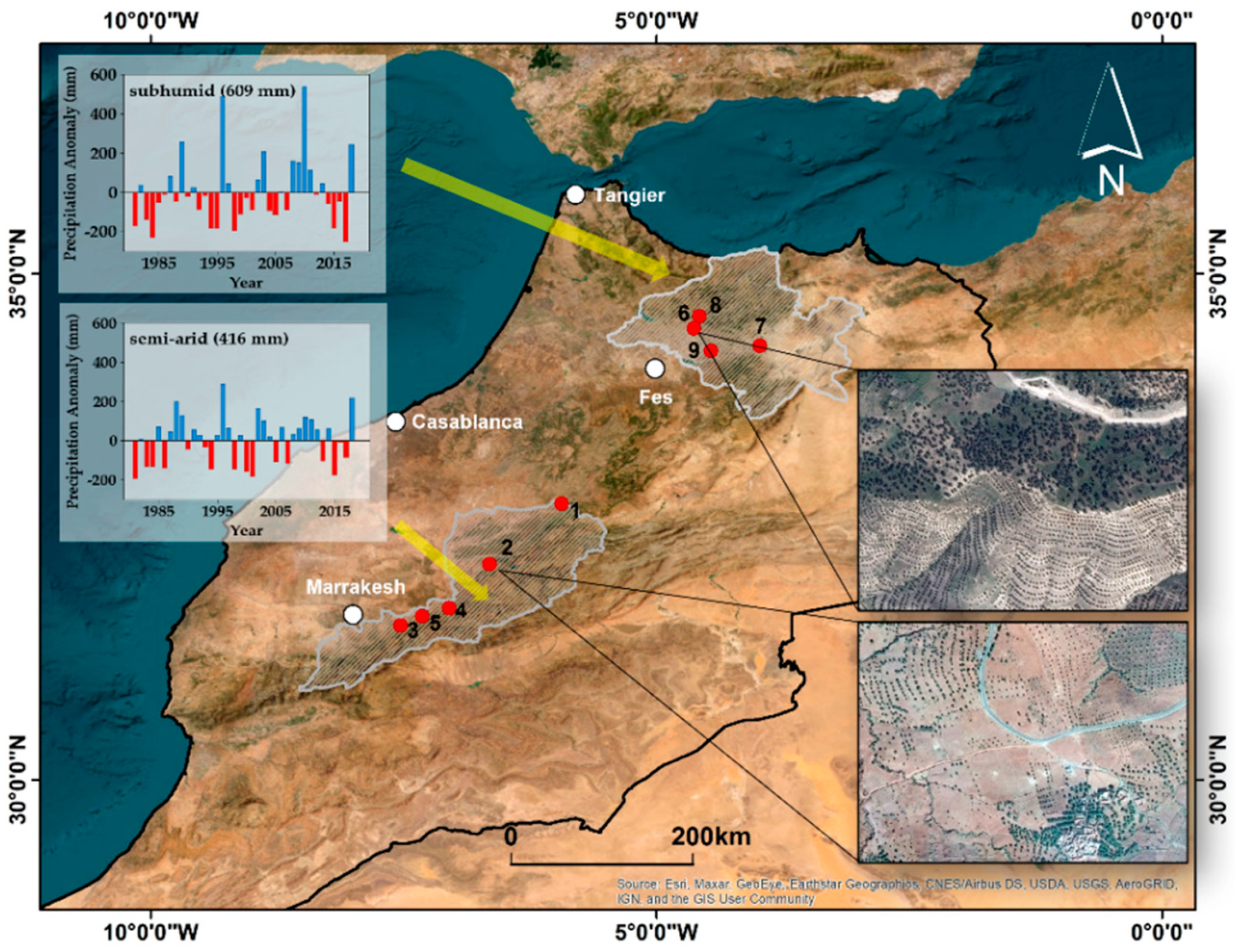
Olive orchards in Morocco are planted in diverse landscapes, varying from semi-arid to humid hilly areas from southwest to northeast. Such gradients result in differences in olive size and spacing both across and within different regions. To represent the spatial variability, we selected nine sites with areas ranging from 1100 to 2500 ha from two contrasting regions that have received investments for olive orchard plantings by the Green Morocco Plan (Figure 1). The sub-humid northern region, Taza-Al Hoceima-Taounate (hereafter, the sub-humid region), has a long history of olive cultivation and exhibits diversified production techniques. The southwestern region, crossing Al Haouz and Azilal, is drier and hillier (hereafter, the semi-arid region) where irrigation systems are more common than in the northern region. Based on the Climate Hazards Group InfraRed Precipitation with Station data (CHIRPS), mean annual precipitation (1980–2018) is approximately 609 mm and 416 mm in the sub-humid and semi-arid regions, respectively, but high inter-annual variability in precipitation has been observed in both regions. Among the nine sites, five are in the semi-arid region and four are in the sub-humid region. To capture the texture variations caused by olive age, the nine sites include both young olive orchards planted through the GMP between 2008 and 2013 and older and larger trees planted between the 1960s and 2000s. All olives were typically planted in systematic rows, either parallel or perpendicular to topographic contours or in rows and columns. Details of the nine sites are displayed in Table 1. Percentages of olive orchards reveal that olives are more widely planted in places where there is ample precipitation. Elevation information of each site is provided in Table S1. Overall, the four sub-humid sites have more topographical variation than the five semi-arid sites.
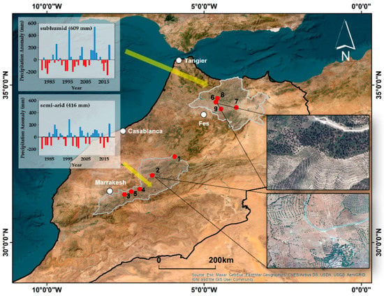
Figure 1.
Map of the Northern part of Morocco and study sites. Subfigures show representative precipitation relative to the average from 1980–2018 (CHIRPS) and example images from DigitalGlobe (spatial resolution of 0.5 m). Red dots show nine sites of olive orchards from paper-based maps available from the Green Morocco Plan.

Table 1.
Site-specific information. Non-olive includes all other land cover types except for olives, such as other vegetation, barren lands, and croplands etc. Olive percentages are derived from visual interpretation of DG imagery (see Section 3.1.2).
2.2. Satellite Data
2.2.1. DigitalGlobe Imagery
DigitalGlobe (DG) is the owner and operator of several VHR commercial satellites, including WorldView (1–3), QuickBird, and IKONOS etc., [45]. In this study, nine analysis-ready images consisting of WorldView-2 and WorldView-3 acquired between 2018 and 2019, were obtained through DG. These products embody a high level of image preprocessing, including radiation correction, inter-sensor calibration and orthorectification, and finally, generation of 8-bit Top of Atmosphere (TOA) radiance with Universal Transverse Mercator (UTM) projection coordinates [46]. All images were pan-sharpened, with 3 bands in nature colors (RGB) and 0.5/0.3-m resolution for WorldView−2/3. To match the spatial resolution, imagery from WorldView-3 was resampled to 0.5 m using the bilinear resampling technique in ArcGIS. The DG imagery of nine study sites is displayed in Figure S1.
2.2.2. Planet Imagery
Planet Lab’s PlanetScope constellation operates more than 135 CubeSats in 2020, which provides consistent global observation daily at a 3-m resolution [47]. In this study, one Planet image was obtained for each site in each month (hereafter as the “time step”) from September 2018 to August 2019 and was cropped to the study area [48]. All images are at level 3B, meaning products with radiation correction, atmospheric correction and orthorectification, and projection to the UTM coordinate system. We used the 16-bit, four-band (Red, Green, Blue and NIR) surface reflectance (SR) data for all image analysis. Note that the original ground sample distance (GSD) of Planet imagery is about 3.7 m and the pixel size is resampled to 3 m after orthorectification [49,50].
To match imagery from DG and Planet, image registration was performed and all three bands of DG imagery (i.e., RGB) and all four bands of Planet imagery (i.e., RGB + NIR) were normalized to −1 and 1 before applying deep learning models. Details of imagery characteristics can be found in Table 2 and acquisition dates of all imagery are shown in Table S2.

Table 2.
Remote sensing imagery characteristics
2.3. Methodology Overview
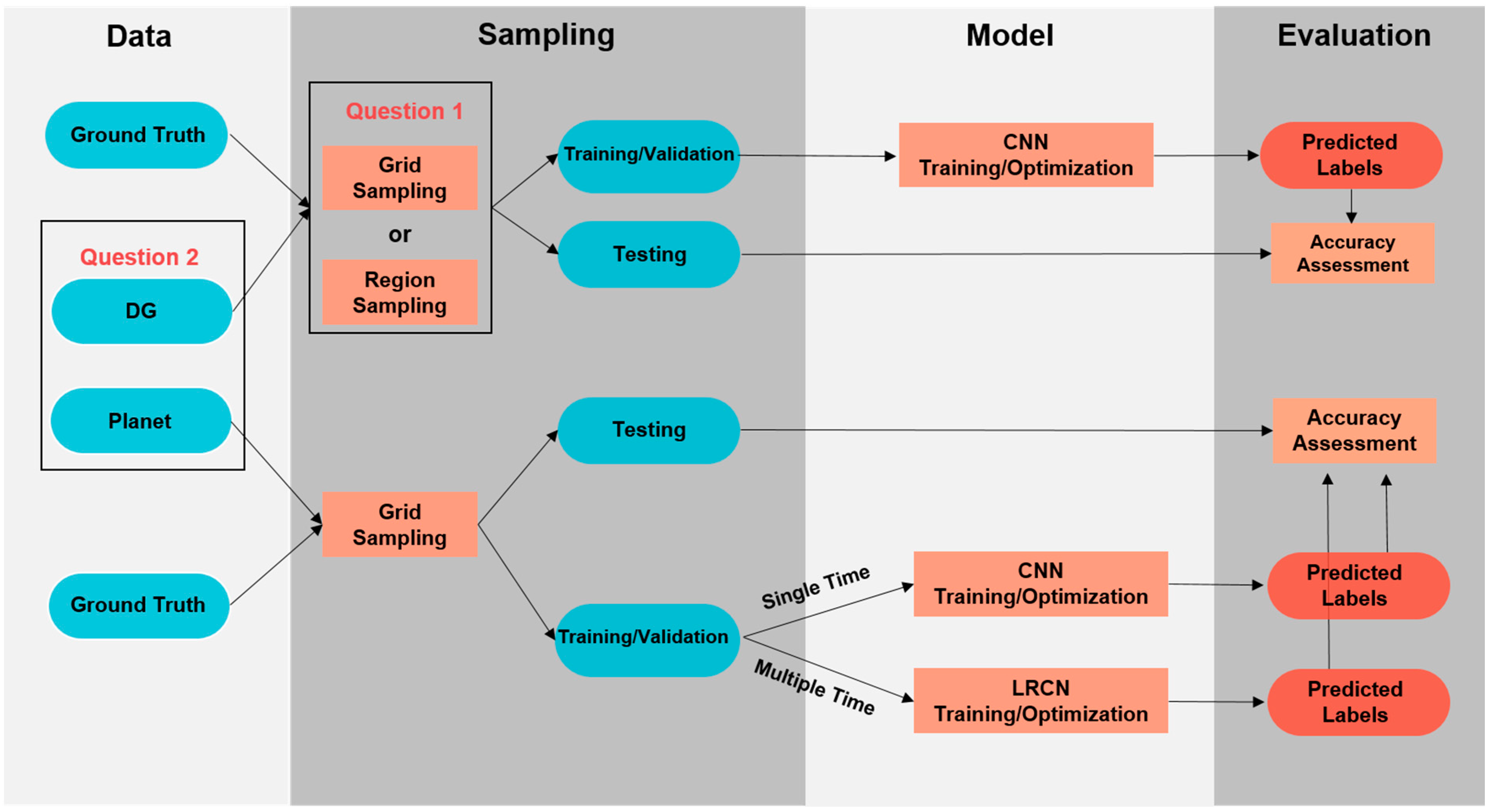
Before diving deep into the details, we briefly overview our methodology in Figure 2. For DG imagery, satellite imagery and ground truth were first divided into training, validation, and testing using different sampling approaches. Next, for each sampling approach, CNN models were trained and optimized using training and validation datasets and evaluated using a testing dataset. These experiments aim to explore the question that how transferable is the model under different levels of spatial variability. For Planet imagery, two different ways of leveraging its multi-temporal information were used. First, CNN models were applied to single time imagery of each time step to find the time step with the best mapping performance for each site. Second, a long-term recurrent convolutional network (LRCN) model was applied to the multi-temporal imagery to utilize the spatiotemporal information simultaneously. The comparison between results of DG and Planet imagery will answer the question that how effective multi-temporal HR imagery is compared to VHR imagery?
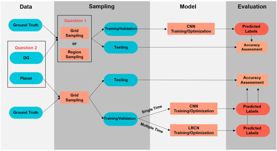
Figure 2.
A flowchart overview of methods used in this study.
2.4. Data Preparation and Pre-Processing
2.4.1. The Logic Behind Patch-Based Classification
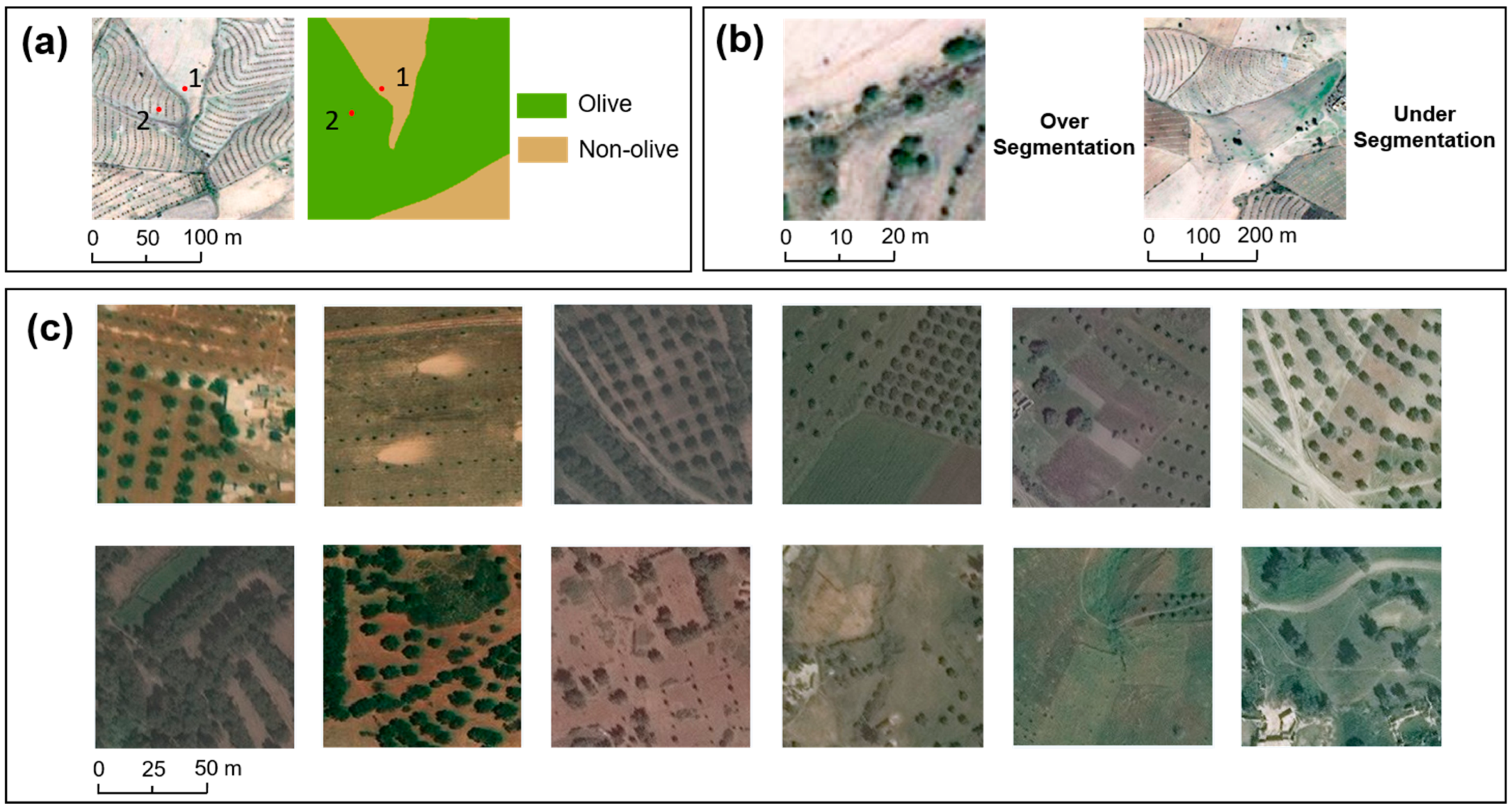
Pixel-based and patch-based classification are two mainstream strategies in image classification tasks [51,52]. Pixel-based classification focuses on labelling individual pixels, which is popular in applications with coarse resolution satellite imagery but shows limitations with VHR images [53,54,55,56]. Specifically, in VHR images, target objects are bigger than the spatial resolution and are thus composed of many pixels [55]. In this case, pixel-based classification becomes problematic because all pixels composing the target collectively contribute to the spatial and spectral characteristics of the object and single pixels lack interpretability for the object. Figure 3a illustrates how pixel-based classification loses efficiency in the high-resolution case. The class “olive” contains olive trees and soil and the uniformly distributed olive trees and soil between each tree together form the unique texture feature of olive orchards. When pixel-based classification is performed, it is challenging to distinguish two soil pixels (i.e., point 1 and 2) belonging to two classes as the two pixels have similar spectral features and possibly similar spatial feature because point 1 is close to the olive orchard. In contrast, patch-based classifications circumvent this issue by assigning labels based on features of an image patch instead of a single pixel, in which case all pixels in the patch together represent the target object. For example, olive orchards can present stronger texture features at the patch level, e.g., they are typically planted in systematic rows. Therefore, we use a patch-based classification in this study. Considering that a good patch size should balance the tradeoff between over-segmentation (i.e., with too limited spatial information to represent the target object) and under-segmentation (i.e., with too much information that will obscure the target object) (Figure 3b) [57], we used (9216 m2) and (9216 m2) pixels as the input image size for DG and Planet after testing different sizes, respectively. The two patch sizes also make DG and Planet patches have the same area, increasing the fairness and effectiveness of the comparison between the two.
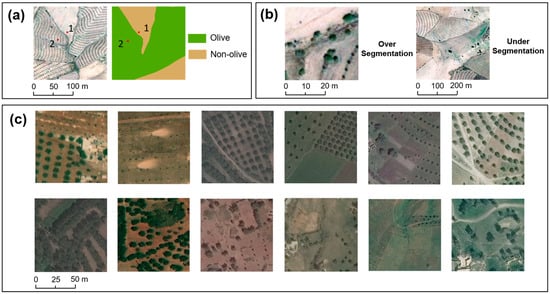
Figure 3.
(a) Pixel-based classification can be problematic in VHR imagery. For example, points 1 and 2 are two soil pixels having similar features but belong to two classes, which make it challenging for pixel-based classification to distinguish the two; (b) over-segmentation (i.e., with too limited spatial information to represent the target object) and under-segmentation (i.e., with too much information that will obscure the target object); (c) olive patches and non-olive patches of varying morphology (first row: olive, second row: non-olive).
2.4.2. Ground Truthing and Labelling
To label olives at the patch level, we used paper-based planning maps of GMP that show locations planted to olive orchards (personal communication, David Mulla) as ground truth. Based on the paper map, electronic ground truth maps for all sites were produced by visual interpretation of DG imagery, which is binary and indicates olive and non-olive pixels. Subsequently, for each site, the DG-derived ground truth map along with the DG imagery were split into non-overlapped pixel patches. Thus, each DG image patch has its corresponding ground truth patch.
As the patch-based classification requires only one label for the entire patch whereas the ground truth patch provides pixel-wise labels, to meet this requirement, one unique label was then determined for the DG image patch based on its corresponding ground truth patch. Specifically, for each DG image patch, if the fraction of olive pixels in the ground truth patch was larger than 30%, the image patch was labelled as olive. A threshold of 30% was used because we wanted to keep more patches located at the edge of olive orchards and maintain sufficient texture features at the same time.
Afterwards, a double visual check was performed for all labelled image patches in the previous step. In a few cases, changes were made if there was a conflict between the label generated from the previous step and the human visual check. For example, a patch with very few or even no olives may be labelled as olives based on the 30% threshold, due to the difficulty of excluding all regions with only sparsely planted olives inside an extensive olive orchard during the visual interpretation. Some examples of olive patches and non-olive patches are shown in Figure 3c. Because each pixel DG patch and pixel Planet patch are geographically registered, the label for each DG image patch was assigned for the corresponding Planet image patch.
2.4.3. Sampling Approach: Different Ways of Allocating Training, Validation, and Testing Dataset
For image classification, training and validation datasets work together to optimize the model and the testing set evaluates the performance of it [58]. The rule of thumb for dataset partitioning is to keep datasets coming from identical distributions [59]. However, due to the spatial variability, ground objects at different geographical locations are prone to have distribution shifts. Consequently, spatial variability has long been concerned to impair model generalizability [60,61,62]. In our case, spatial variability is two-fold: interregional variability and intraregional variability. The former indicates the variability between the sub-humid region and semi-arid region and the latter represents the variability within the sub-humid region or semi-arid region. Ref [61] argued that interregional variability was the main cause for poor model generalizability, and suggested building separate models for regions that are homogenous in certain features. Following this, we built models for two climatic regions separately. However, the impact of intraregional variability remains underexplored. This is largely due to the wide use of the simple random sampling approach that draws samples with equal opportunity regardless of their spatial locations. This complete randomness can significantly reduce the spatial variability. For example, a training sample can be exactly next to a testing sample and the two samples can have high spatial autocorrelation. As spatial variability is not quantitatively measurable, the challenge of evaluating the influence of intraregional spatial variability is how to control the degree of it. To address that, we employed two variants of the random sampling approach with different spatial constraints, i.e., grid random sampling (hereafter as the “grid sampling”) and region random sampling (hereafter as the “region sampling”). The underlying assumption is that the degree of spatial variability should be proportional to the distance, i.e., the first law of geography [63].
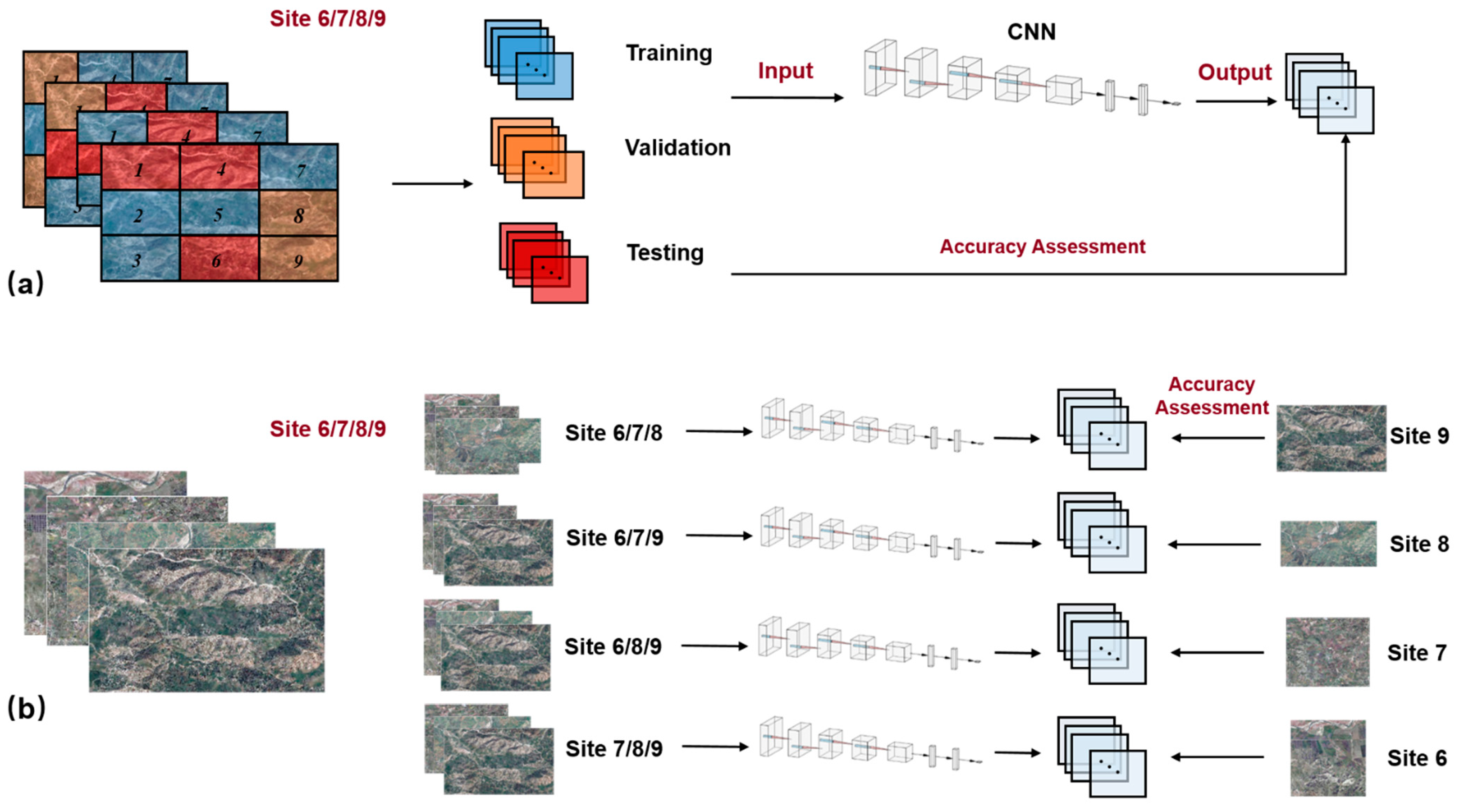
Figure 4a illustrates how grid sampling works using the four sub-humid sites as an example. We split each of the four sites into nine equal-sized grids from the upper left corner to the lower right corner. Among the nine, four are used for training (blue grids), two for validation (orange grids) and three for testing (red grids). Compared to the simple random sampling approach that draws samples with equal opportunity regardless of their spatial locations, using separated grids as the spatial constraint helps reduced adjacency and preserves spatial variability among training, validation, and testing dataset. However, even though we confine the sampling using grids, grids inevitably will have adjacencies. For example, testing grids 1, 4, 6 in Figure 4 have connections with training grids 2, 3, 5, and 7. Therefore, the grid sampling approach will only retain weak spatial variability because it helps reduce spatial autocorrelation among samples compared to the simple random sampling but cannot eliminate all spatial autocorrelation.
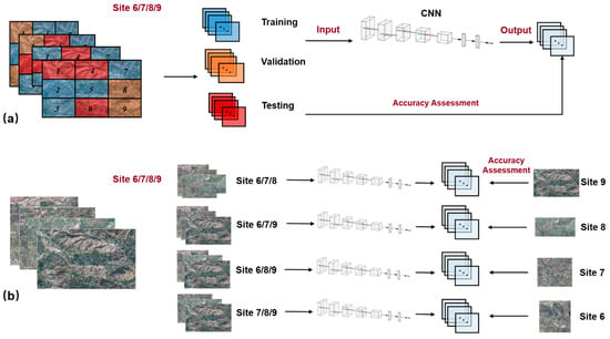
Figure 4.
Frameworks of two sampling approaches (see Figure 7 for details of the CNN architecture). (a) Grid sampling; (b) region sampling.
Detailed information about grid-sampling partitioning is shown in Table 3. Note that grids assigned for training, validation, and testing have comparable olive and non-olive ratios.

Table 3.
Index of training, validation, and testing grids in each site.
For the region sampling (Figure 4b), all but one of the four sites were used as training and validation every time, while the excluded site was used for testing. Thus, each site has its individual model. This is different from the grid-sampling approach where all sites in each climate region contribute to training one model. As different sites are isolated from each other (Figure 1), the spatial autocorrelation becomes negligible. Thus, the region sampling approach can generate training, validation, and testing dataset with stronger spatial variability compared to the grid-sampling approach.
2.5. Olive Orchard Mapping with Deep Learning
2.5.1. Difference between Olive Orchards in DG and Planet Imagery
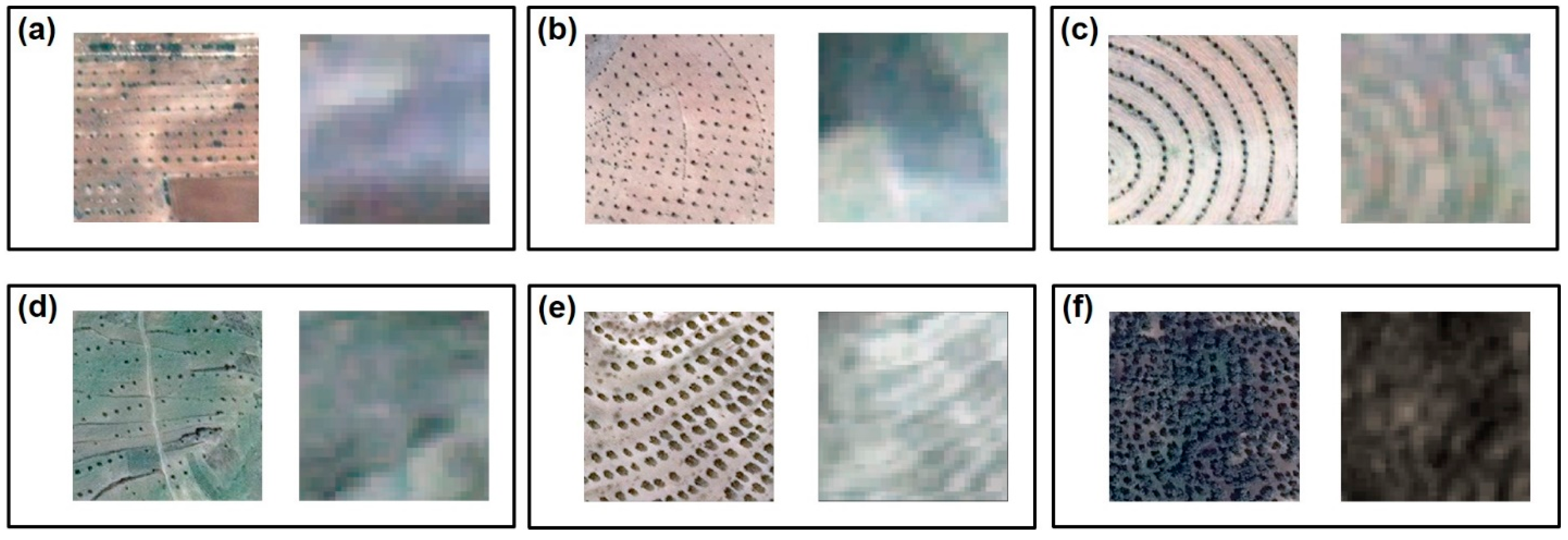
As illustrated by Figure 5, the gap in the spatial resolution (0.5 m for DG versus 3 m for Planet) leads to a large difference in spatial information contained in the image. All six DG patches show sufficient information to distinguish between olives and non-olives whereas Planet patches have limited capacity to accurately represent the two categories due to the reduction of spatial resolution. The first row of Figure 5 is selected from the semi-arid region where most olives become invisible on Planet imagery because of the small canopy size relative to the spacing between adjacent olive trees. In some cases, Planet imagery shows detectable features of olives (Figure 5c) and in others, it does not (Figure 5a,b). The second row is from the sub-humid region. While small size olives remain a challenge (Figure 5d), a larger portion of olives in this area have larger sizes and can be captured by the Planet imagery (Figure 5e). Additionally, due to sufficient precipitation, lush natural vegetation occasionally presents features similar to olives (Figure 5f).
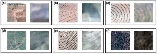
Figure 5.
The difference in olive orchards with DG (left) and Planet imagery (right). (a–c) are from the semi-arid region, (d–f) are from the sub-humid region. (a,b) show areas where olives are visible on DG imagery but not on Planet imagery due to small crown sizes; (c) shows the case where olives are visible both on DG imagery and on Planet imagery; (d) shows the case where olives are visible on DG imagery, but not on Planet imagery due to small crown sizes; (e) shows the case where olives are visible both on DG imagery and on Planet imagery; (f) shows the case where non-olive vegetation shows similar features as olives on Planet imagery.
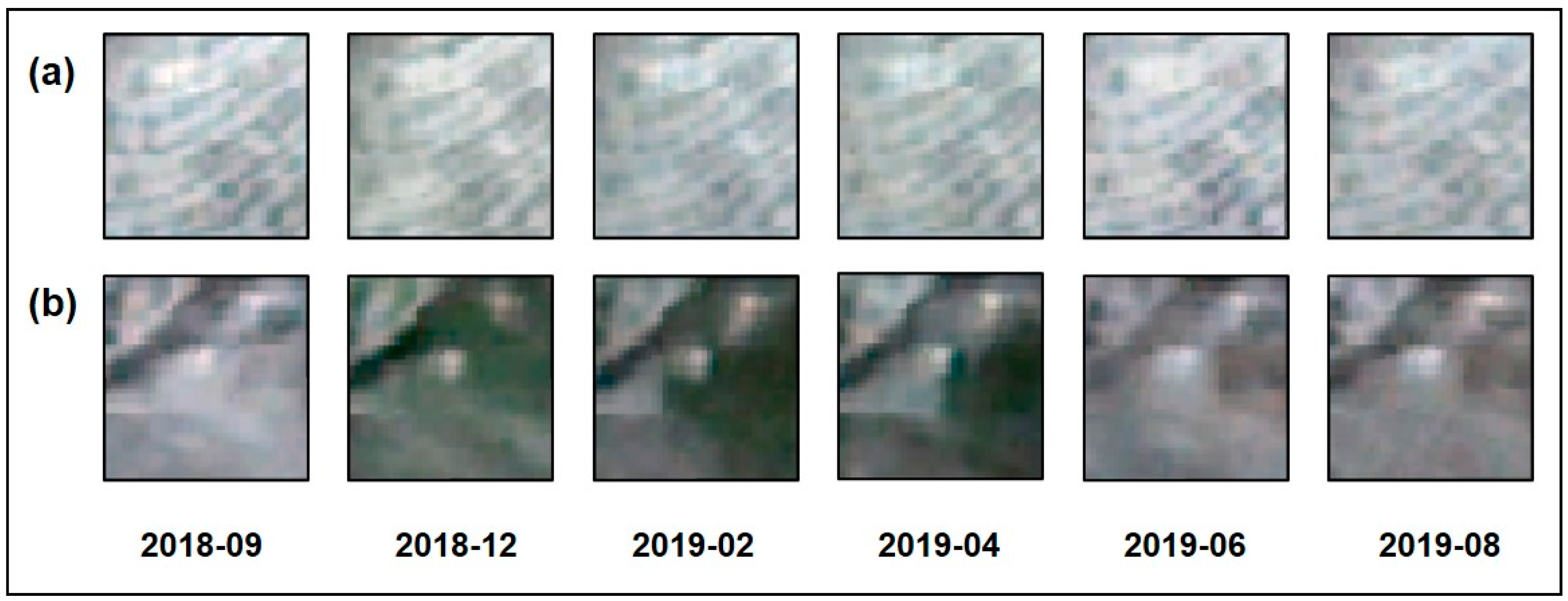
Comparison in Figure 5 indicates that DG imagery contains sufficient spatial features to detect olive orchards whereas Planet imagery show varying capacities in different cases. However, benefiting from the high temporal resolution of Planet imagery, one image was obtained for each site in each month of the growing season of 2019, i.e., from September 2018 to August 2019. Figure 6 displays temporal changes of an olive and a non-olive patch. Olives do not show significant temporal variation (Figure 6a) but some non-olives, such as annual plants, shows periodical changes over time (Figure 6b). The difference between Figure 6a,b suggests that introducing temporal information can potentially help differentiate annual plants from olives and offset the loss of spatial information of Planet imagery.
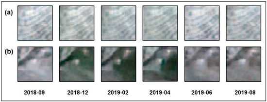
Figure 6.
Temporal change of olives and non-olives on Planet imagery. (a) Olives have stable features over time; (b) some non-olives show intra-annual phenological change.
Due to the different characteristics of DG and Planet imagery, the experiment-designing is different for the two data. For DG imagery, only CNN models were used to take advantage of its high spatial resolution. For Planet imagery, not only were CNN models trained for each time step to find the time step with the best performance for each site, but also the LRCN models were applied using multi-temporal imagery to utilize the spatiotemporal information at the same time.
Note that since developing more advanced algorithms is not a focus of this study, we selected existing CNN and LRCN models for the mapping the tasks as those types of architecture have proven to be powerful tools in discriminating spatial and temporal features for land classification and avoid huge feature engineering work required by traditional algorithms such as random forest and support vector machine.
2.5.2. CNN Model
CNN is a group of deep learning architectures that are quite popular in image classification and segmentation due to its powerful capacity for learning features with a series of operations like convolution and pooling. Since the appearance of the first CNN in 1998 [34], CNN has been undergoing drastic changes in terms of the layer depth, width, and addition of functional components [35,64,65,66] and has progressively substituted for traditional machine learning algorithms, e.g., random forest, to be the main tool for remote sensing image classification.
Although CNN models with increasingly deeper and ingenious architectures have been proposed for addressing more complex classification, segmentation, or identification problems, they may not necessarily perform better [19]. After testing different CNN architectures from simple to complex, we built a VGG-alike network for the relatively simple binary classification task (i.e., olive versus non-olive) in this study [64]. The reasons are two-fold. First, compared to simpler architectures, e.g., LeNet and AlexNet, this VGG-alike network showed more powerful capacity in mapping olive orchards. Second, it is computationally efficient in terms of the number of parameters, e.g., 30,591 vs. 11,177,025 (ResNet-18 [66]) and employing complex architectures (ResNet and DenseNet [67]) did not show any improvement to the result. Hyperparameters, e.g., learning rate and batch size etc., were adjusted continuously until they achieved the best performance (Table S3). The detailed architecture of the CNN model is given in Figure 7. Components 1 to 5 indicate two convolutional blocks with each containing a BatchNorm-Conv-LeakyRelu sequence. The filter size of the convolutional layer is . Component 6 and 7 are two fully connected layers. For components 1 to 5, a MaxPooling layer is used between any of the two components and an AveragePooling layer is used between component 5 and 6.

Figure 7.
CNN architecture (taking DG patches as input). Each convolution block contains two BN-Conv-LR sequences. A max pooling is used between any two of the convolutional blocks. A global average pooling is added between component 5 and 6. Two fully connected layers and one sigmoid layer are followed after convolutional layers.
2.5.3. LRCN Model
To fully take advantage of the temporal information provided by Planet imagery, a LRCN model was applied to the multi-temporal data [68]. LRCN is a variant of the long short-term memory (LSTM) network, which is a widely used recurrent neural network (RNN) to address sequence learning problems and existing studies have already shown its outperformance in processing time-series imagery over CNN and traditional machine learning algorithms [69,70,71].
A LRCN consists of a CNN component and a LSTM component. A CNN encoder is applied to extract the spatial information before inputting to the LSTM. Therefore, a LRCN model can capture spatiotemporal information of Planet imagery simultaneously. To make a fair comparison with results using CNN and single time step Planet imagery, the same VGG13-alike model was used as the CNN encoder. A LSTM component was inserted between components 5 and 6 in Figure 7 to extract temporal information of the input vector that contains spatial information of multi-temporal Planet imagery.
Note that due to the number of olive patches being unequal to that of non-olives, different weights were assigned to the loss function during training. Minority class thus has a higher weight, indicating a higher penalty when misclassifying it. When training the network, we applied the Adam optimizer to minimize the weighted binary cross-entropy loss [72,73], the equation of which is defined as:
where , , , and were the loss, label, model output, and weight for the batch . The average loss of all batches was finally used to optimize the model:
where is the number of batches, is the total loss for all batches.
All experiments were conducted with PyTorch on a Dell workstation with 64 GiB Intel(R) Xeon(R) W-3250 CPU @ 4.00 GHz, 11 GiB RTX 2080 Ti GPU, and 64-bit Windows 10 OS.
2.6. Accuracy Assessment
Accuracy evaluation was performed using three metrics, precision, recall, F1 score, and overall accuracy (OA) [74,75,76]. The definitions are:
where , , , and indicate true positive, false positive, true negative, and false negative, respectively. In this study, true positive represents the case where both the prediction and label are olives, false positive represents the case where the prediction is olive but the label is non-olive. The same logic can apply to true negative and false negative.
Among the four metrics, precision and recall reflect the portion of correctly identified olives and the portion of actual olives that are correctly identified; F1 score is the harmonic mean of precision and recall; OA indicates an overall performance of the classification result.
3. Results
3.1. Mapping Olive Orchards Using 0.5 m DG Imagery
3.1.1. Results Using DG Imagery and Grid Sampling
Table 4 shows the accuracy evaluation for the grid sampling approach. In the semi-arid region, the mean precision, recall, and F1 score are 0.87, 0.89, and 0.88. In the sub-humid region, both mean precision and recall have higher values than the semi-arid region and correspondingly, higher F1 score. In terms of the OA, the semi-arid region has a higher mean OA than the sub-humid region because non-olives account for a larger percentage. Therefore, the OA can reach a high value when most non-olives are correctly identified.

Table 4.
Evaluation metrics for olive orchard mapping using grid sampling with DG imagery (TP: true positive, FP: false positive, TN: true negative, FN: false negative).
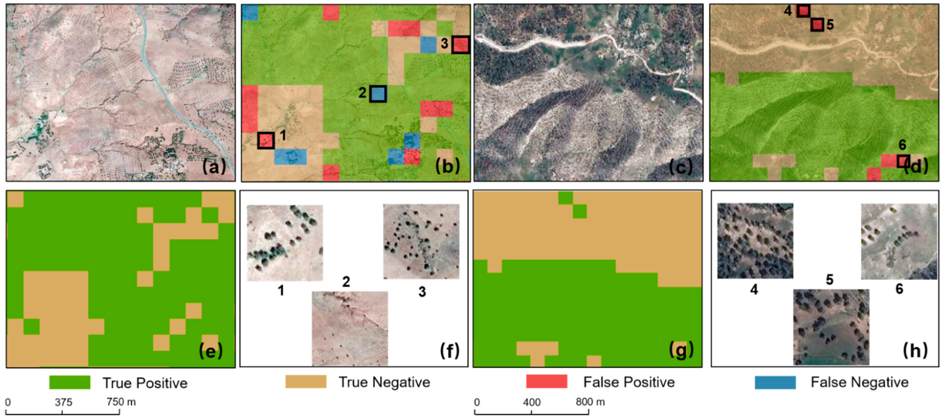
Figure 8 gives a visualization of misclassifications between olives and non-olives. Figure 8e,g displays the raw classification map without pointing out the locations with false positive/negative and true positive/negative. Patches 1 and 3 in Figure 8f show cases where non-olives with similar texture features as olives in the semi-arid region were classified as olives. Patch 2 in Figure 8f indicates that olives located at the edge are more likely to be omitted and be classified as non-olives. Patches 4, 5, and 6 in the sub-humid region (Figure 8h) present the same problem shown in patches 1 and 3, which is misclassification caused by other vegetation that presents olive-like texture features.
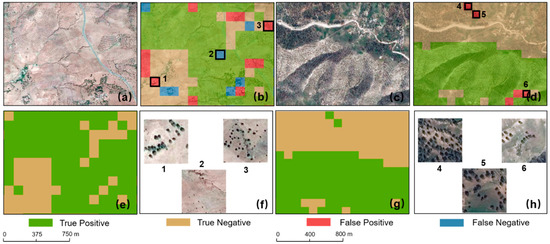
Figure 8.
Olive mapping results using the grid sampling approach and DG imagery. The legend only applies to (b,d). (a) RGB imagery in grid 5, semi-arid site 5; (b) classification map showing TP/TN/FP/FN in grid 5, semi-arid site 5; (c) RGB imagery in grid 4, sub-humid site 9; (d) classification map showing TP/TN/FP/FN in grid 4, sub-humid site 9; (e) classification map in grid 5, semi-arid site 5; (f) examples for false positive and false negative values in grid 5, semi-arid site 5; (g) classification map in grid 4, sub-humid site 9; (h) examples of false positive and false negative values in grid 4, sub-humid site 9.
3.1.2. Results Using DG Imagery and Region Sampling
Two evaluations were used for models based on the region sampling approach. The first evaluation only used the three testing grids (displayed in Table 3) in each site to make a direct comparison with the result of grid-sampling (Table 4). Results in Table 5 show that models trained with grid-sampling outperform models trained with region-sampling. F1 scores and OA of two regions drop from 0.88 to 0.84, 0.90 to 0.88, 0.94 to 0.93, and 0.92 to 0.91, respectively. For the second evaluation, testing sets are enlarged from three grids to the entire site, which will introduce more spatial variability. Table 6 shows a further performance reduction compared to Table 5. F1 scores and OA of two regions change from 0.84 to 0.83, 0.88 to 0.85, 0.93 to 0.92, and 0.91 to 0.88.

Table 5.
Evaluation metrics for olive orchard mapping using region sampling with DG imagery (1st evaluation).

Table 6.
Evaluation metrics for olive orchard mapping using region sampling with DG imagery (2nd evaluation).
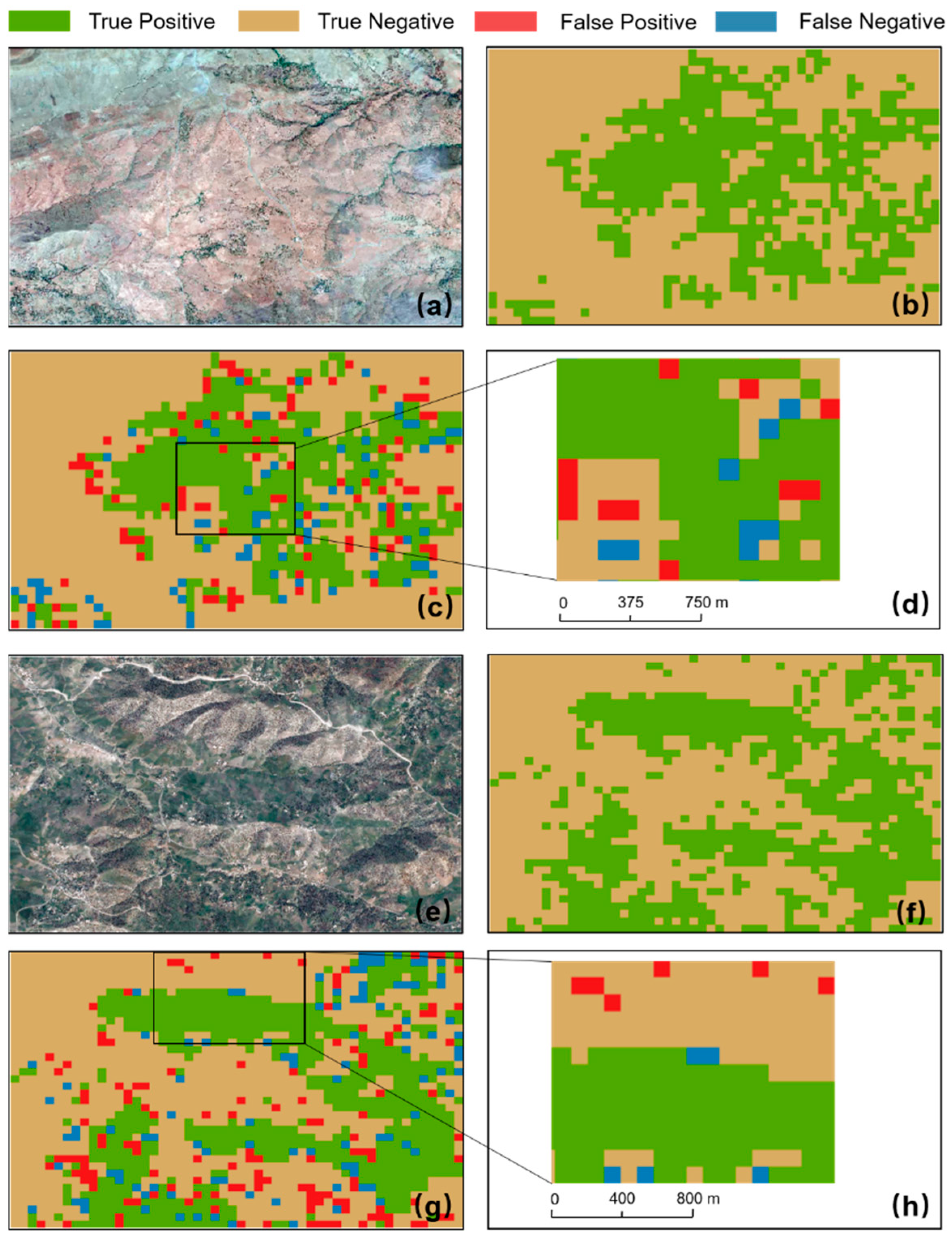
Figure 9 shows an example of olive orchard maps using the region sampling approach. Figure 9d,h shows the same grids as in Figure 8b,d that uses the grid-sampling approach. Compared with the results in Figure 8, Figure 9d,h shows more false positive (red) and more false negative (blue) values, which coincide with lower precision and recall values when using the region-sampling approach.
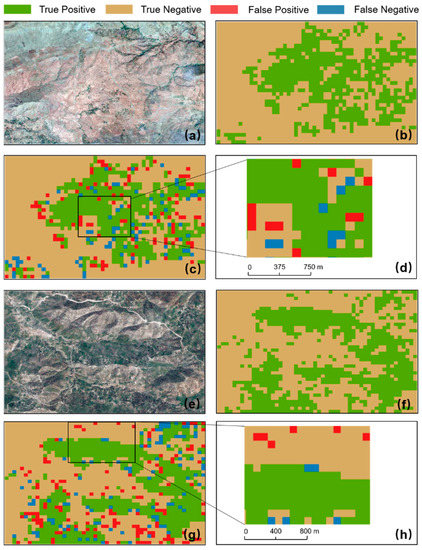
Figure 9.
Olive mapping results using the region sampling approach and DG imagery. The legend only applies to (c,d,g,h). (a) RGB imagery in semi-arid site 5; (b) classification map in semi-arid site 5; (c) classification map showing TP/TN/FP/FN in semi-arid site 5; (d) classification map showing TP/TN/FP/FN in grid 5, semi-arid site 5; (e) RGB imagery in sub-humid site 9; (f) classification map in sub-humid site 9; (g) classification map showing TP/TN/FP/FN in sub-humid site 9; (h) classification map showing TP/TN/FP/FN in grid 4, sub-humid site 9.
3.2. Mapping Olive Orchards Using 3-m Planet Imagery
3.2.1. Results Using Single Time Planet Imagery and CNN
Table 7 shows the best result that single time Planet imagery could achieve among the 12 time steps for each site, which has poorer performance compared to DG imagery. The five semi-arid sites consistently have low values of precision, recall, F1 score, and OA, which are on average 0.26, 0.42, 0.32, and 0.59, respectively. Since a larger portion of olives in the sub-humid region is with older ages, larger crowns, and wider spacings, the expectation for this region is higher values in all metrics than the semi-arid region. The result coincides with this and the average precision, recall, F1 score, and OA are 0.55, 0.56, 0.55, and 0.66, respectively.

Table 7.
Evaluation metrics of olive mapping using single time Planet imagery using CNN.
Compared to the result using DG imagery shown in Figure 8, Figure 10 further reveals the limitations of Planet imagery in olive orchard mapping visually. First, fewer olive trees with distinguishable features were correctly detected (patch 3 in Figure 10f, patch 6 in Figure 10h). Second, olive trees with no distinguishable features and non-olives were misclassified mutually (patch 1, 2 in Figure 10f, patch 4, 5 in Figure 10h). Third, trees in the shaded area were mostly obscured compared to the VHR DG imagery, e.g., patch 4 in Figure 10.
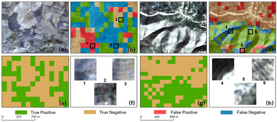
Figure 10.
Olive mapping results using the grid sampling approach and Planet imagery. The legend only applies to (b,d). (a) RGB imagery in grid 5, semi-arid site 5; (b) classification map showing TP/TN/FP/FN in grid 5, semi-arid site 5; (c) RGB imagery in grid 4, sub-humid site 9; (d) classification map showing TP/TN/FP/FN in grid 4, sub-humid site 9; (e) classification map in grid 5, semi-arid site 5; (f) examples for false positive and false negative values in grid 5, semi-arid site 5; (g) classification map in grid 4, sub-humid site 9; (h) examples of false positive and false negative values in grid 4, sub-humid site 9.
3.2.2. Results Using Multi-Temporal Planet Imagery and LRCN
The assumption for this experiment is that multi-temporal information can help improve misclassifications occurring when using single-time Planet imagery. However, results in Table 8 reveal that the detection of non-olives has improved whereas olives may or may not benefit from the multi-temporal information under different cases. In the semi-arid region, more olive patches were misclassified compared to Table 7 (lower TP and higher FN) but fewer non-olive patches were misclassified (higher TN and lower FP). Therefore, the average precision is higher (0.40 versus 0.26) but recall (0.27 versus 0.42) is lower. In the sub-humid region, as a positive case where multi-temporal information benefits detections of both olives and non-olives, higher values of precision (0.65 versus 0.55) and recall (0.64 versus 0.56) are observed.

Table 8.
Evaluation metrics of olive tree mapping for Planet imagery using LRCN and multiple time steps.
4. Discussion
4.1. Difference between Olive Orchard Mapping in Semi-Arid and Sub-Humid Regions
According to Table 4, the mean precision and recall in semi-arid region are 0.87 and 0.89, indicating that on average 13% of the identified olives are in reality non-olives, while 11% of olives were misclassified as non-olives. Albeit values of two metrics are comparable, considering the larger portion of non-olives in dry areas (i.e., 119 out of 2935 non-olive patches were misclassified whereas 100 out of 882 olive patches were misclassified), olive detection is more challenging than non-olives. This is consistent with the fact that olives in drier areas were mostly planted after 2008 with just a few olive groves having decades-old ages. Therefore, most olives with small crown sizes bring challenges for their detection. Meanwhile, the large spacing between olive trees relative to small tree sizes further increases the difficulty. Compared to olives, non-olives in drier sites are more detectable as landscapes have simple and consistent features. Therefore, fewer non-olives were misclassified.
Compared to the results in the semi-arid region, the sub-humid region has a higher mean recall, i.e., 0.92, suggesting that olives in the humid area can be more easily recognized. The reason is that the sub-humid region provides a more favorable environment for olive growth, including sufficient water supply and more fertile soil. As a result, olive planting has a long history in humid areas, and most olives have large enough crown sizes to be easily recognized from satellite imagery. However, the higher mean precision, i.e., 0.88, does not mean non-olives are also easily detectable in this area. Instead, the detection becomes more challenging due to more abundant backgrounds. For example, some natural forests and random trees can occasionally display features similar to olives, which leads to misclassification. Therefore, a higher ratio of misclassified non-olives is observed in the sub-humid region, i.e., 98 out of 1275 versus 119 out of 2935 in the drier area. However, since the absolute value of false positives is smaller (98 versus 119) as well as true positives are comparable (710 versus 782), the precision value becomes slightly higher according to Equation (3).
4.2. Model Generalizability under Different Levels of Spatial Variability
One of the goals is to explore the model generalizability under different levels of spatial variability. To achieve this goal, we employed two sampling approaches, i.e., grid sampling and region sampling, to generate training, validation, and testing dataset. The grid sampling approach represents a weaker spatial variability (Section 2.4.3) and the mean F1 score and OA for two climatic regions are 0.88 and 0.94, 0.90 and 0.92, respectively, based on the datasets generated from it.
As a comparison, the region sampling generates datasets with stronger spatial variability. Results in Table 5 show that when using the same three testing grids in each site, region-sampling is worse than grid-sampling. The loss in precision comes from more confusion between olives and non-olives, i.e., less true positives and more false positives. Simultaneously, as fewer true positives are equivalent to more false negatives, values of recall also drop from 0.89 to 0.85 in the semi-arid region and from 0.92 to 0.90 in the sub-humid region. The loss in precision and recall indicates that variability exists among different sites within the same climatic region. Due to this, for a given site, olives and non-olives with features that are not learned by the model from other sites are less likely to be correctly identified. When enlarging the testing set, more variability was involved and worsened the model performance.
Two experiments using grid and region-sampling together measure to what degree spatial variability will influence model generalizability. In our case, while still yielding satisfying performance, when generalizing models to new data with distribution shift (spatial variability), values of precision, recall, F1 score, and OA could have decreased by up to 0.05, 0.05, 0.05, and 0.04, respectively.
4.3. The Effectiveness of Planet Imagery Compared to DG Imagery
Another goal of this study is to explore the effectiveness of HR imagery compared to the VHR imagery. Results in Table 7 indicate that the single date Planet imagery, even with selecting the best result among 12 time steps, has much poorer performance than DG imagery. This can be attributed to the fact that most olives are invisible on Planet imagery due to the small canopy size relative to the spacing between adjacent olive trees. Patches labelled as olives but with no distinguishable features would likely bias the model, making it incapable of differentiating featureless olive patches from non-olive patches. Consequently, misclassifications occurred frequently between olives and non-olives, i.e., 1061 non-olive and 512 olive patches were misclassified into the opposite category. In the sub-humid region, more detectable features of olives mitigate the confusion between the two classes. Consequently, only 340 out of 768 olive patches and 357 out of 1285 non-olives were misclassified compared to 512 out of 882 and 1061 out of 2935 in the semi-arid region.
Incorporating multi-temporal information also does not necessarily improve the performance. In the semi-arid region, the improvement in non-olive detection can be attributed to the seasonality shown by some non-olives that helps to better recognize the non-olives misclassified as olives using single time imagery. Two reasons may explain the decreased capacity for olive detection. First, only a portion of non-olives in dry areas has annual changes and other portions are featured by more barren lands showing less intensive periodical variations. Since the temporal change for olives is also marginal, incorporating temporal information does not help distinguish olives without obvious texture features from similar barren lands. Additionally, due to the strong seasonal change of non-olives, the weak spatial feature of some olives can be obscured by it if those olives are grown with annual plants such as grasses.
Similarly, the improvement in non-olive detection in the sub-humid region is due to the seasonality of some non-olives. However, differences in the background environment and olive features in the sub-humid region also facilitate the detection of olives. First, there is a larger portion of non-olives in the humid region having seasonal changes, which can help reduce the misclassification from olives. For example, natural forests that display similar texture features. Second, older and larger olives in the humid region have stronger spatial features than younger and smaller ones in the arid region, thus will not be easily obscured by temporal features from surrounding annual plants.
The two experiments using single time and multi-temporal Planet imagery suggest that spatial information, e.g., texture feature, still plays a key role in olive detection. The multi-temporal information can be helpful as an auxiliary force for spatial information, e.g., in the sub-humid region where older trees have obvious texture features. However, if the spatial feature itself is weak, incorporating temporal information may not improve the performance.
4.4. Feature Representation for Olive Orchards
To explore how feature representations relate to the model performance, we visualized features of five convolutional layers of DG and Planet imagery, respectively. This has been proven to be an effective way to know representative features in different tasks, e.g., cropland mapping [58,77] and yield prediction [78].
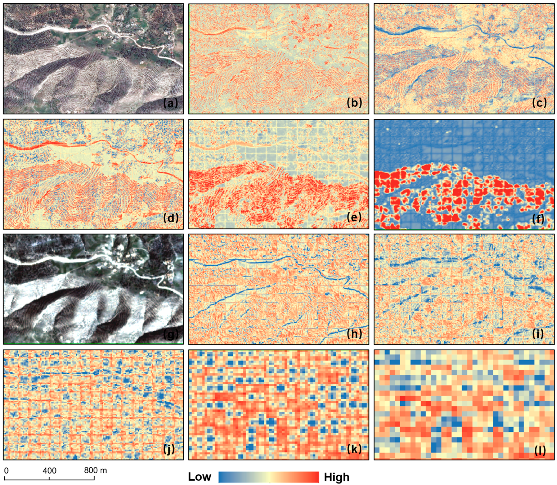
Figure 11 shows an example where the DG-based model learned well but the Planet-based model failed to learn representative features. For the DG-based model, the shape of trees is first learned, and every single tree stands out without differentiating between plantation and natural trees (Figure 11b). From Figure 11b–e, the texture feature of olive orchards is highlighted incrementally with the model forwarding to deeper layers. As a result, in the fifth convolutional layer (Figure 11f), areas with distinct texture features are distinguished from other areas. As a comparison, in Figure 11g, due to younger ages and smaller sizes, most olives show no spatial features on coarser Planet imagery and are confused with non-olives. Therefore, instead of learning some distinguishing features, what highlighted in each layer were common features to the two categories. Consequently, a large extent of misclassification was observed due to the unrepresentative features learned in previous layers (Figure 11I).
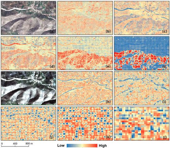
Figure 11.
Feature representations for the olive orchard in grid 5, semi-arid site 5. (a,g) RGB imagery from DG and Planet; (b–f) feature representations of convolutional layer one to five for DG imagery; (h–l) feature representations of convolutional layer one to five for Planet imagery.
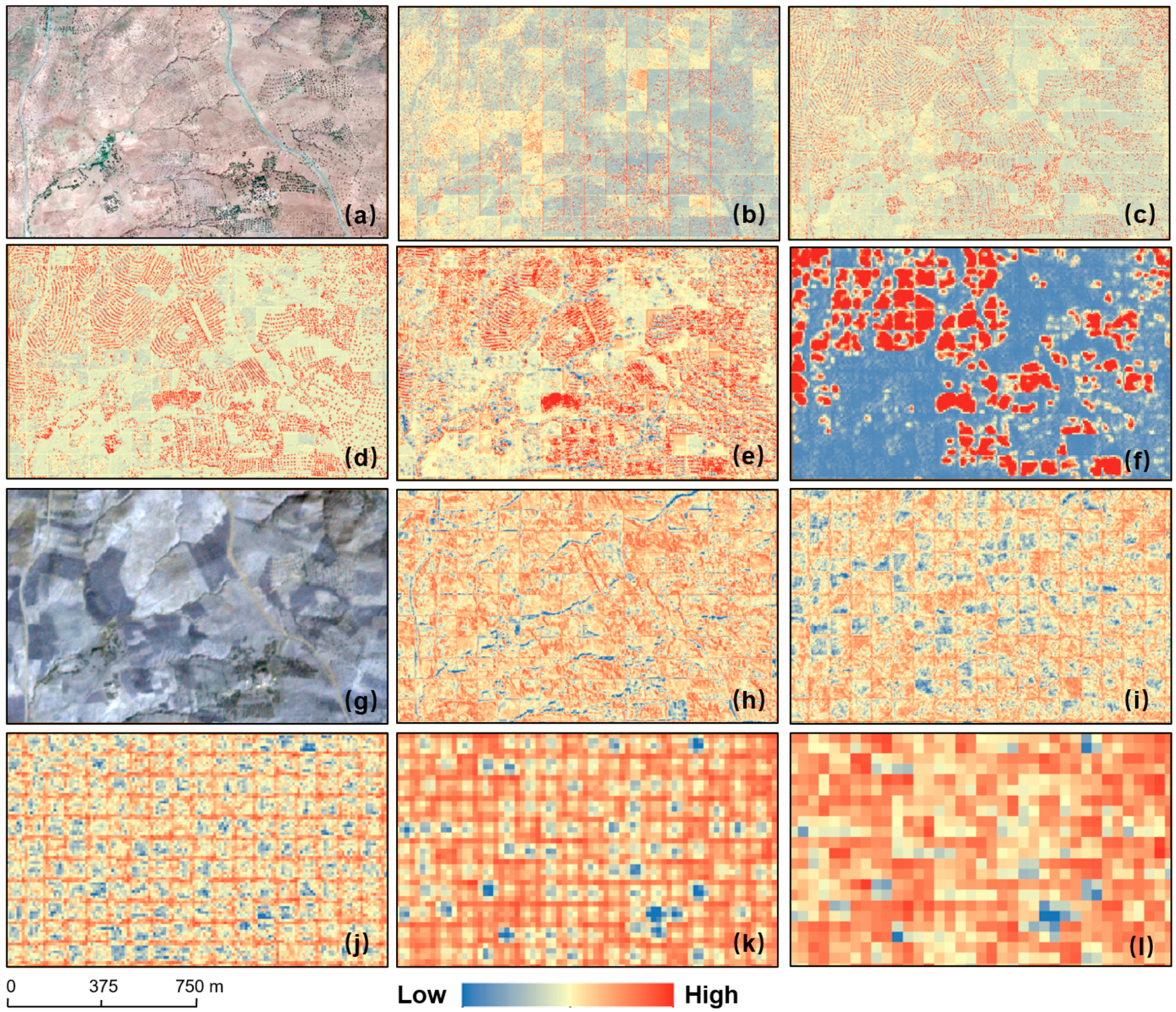
Similarly, in Figure 12a–f, feature representation of each layer of the DG-based model started from low-level features such as the shape of trees to high-level features such as the line texture. Finally, olives planted along the contour were correctly classified. However, in contrast to the unrepresentative features learned by the Planet-based model in Figure 11, the spatial feature of olives was gradually highlighted as the model proceeded to deeper layers. Although confusions were still observed in the upper region where natural forests were grown, the degree of this was reduced compared to Figure 11I. This example reveals that the Planet-based model also learned useful information when olives are older, bigger, and show more detectable spatial features on Planet imagery.
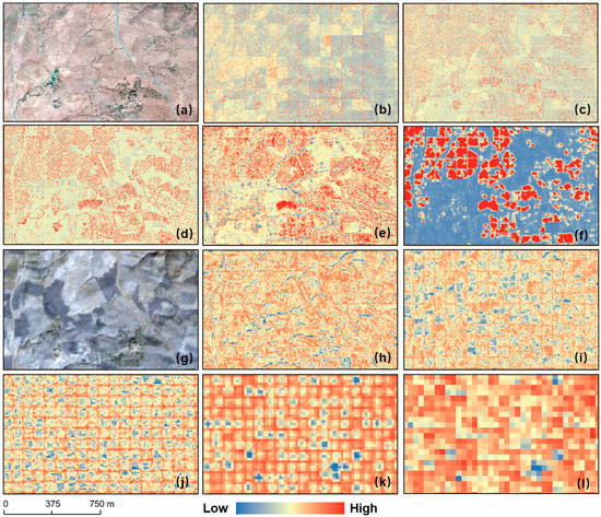
Figure 12.
Feature representations for the olive orchard in grid 4, sub-humid site 9. (a,g) RGB imagery from DG and Planet; (b–f) feature representations of convolutional layer one to five for DG imagery; (h–l) feature representations of convolutional layer one to five for Planet imagery.
4.5. When Is Planet-Alike HR Imagery Effective?
The spatial resolution has been considered as a key factor influencing the performance of remote sensing applications. For example, [79] discussed the effect of spatial resolution on the capacity of satellite imagery to monitor individual fields, [80] emphasized the importance of finer resolution imagery in global land cover mapping. VHR imagery is attractive due to the capability to capture features that are usually omitted by relatively coarser resolution imagery but at the cost of data acquisition and accessibility [28,81]. For example, to obtain single-date imagery covering the entire semi-arid region shown in Figure 1 (approximately 15,000 km2), the cost of commonly used VHR imagery with spatial resolution greater than 0.5 m ranges from ~$150,000 to ~$450,000. As a comparison, the cost of 3 m PlanetScope imagery is about $15,000 [82]. Therefore, although DG imagery has been proven to have consistent good performance in detecting less dense and relatively smaller olive orchards, it is still worthwhile to find out when we should use DG-alike VHR imagery only and when Planet-alike HR imagery can be effective.
A direct answer from previous experiments is that Planet imagery should be used in areas with most olive orchards being distinctly identifiable. Two main factors determine the identifiability of olive orchards on Planet imagery. The primary factor is crown size, which is linked with tree age. As shown in Figure 13a,b, either in the semi-arid or sub-humid region, olives with approximately a diameter of 5 meters have visible texture features on Planet imagery. The second factor, i.e., the spacing between individual olives, explains why olive orchards still show features when crown sizes are relatively small. When spacings between olives are narrow relative to their crown size, the feature of an olive row is more likely to be obvious. For example, the crown size is about 3.5 m while the spacing is less than 3 m in Figure 13c,d, otherwise, it becomes blurry (Figure 13e). Another effect of tree spacing is that olives are generally more densely planted in one direction than in the perpendicular direction. Equidistant tree spacings in all directions for trees with large crowns would cause this texture feature to disappear (Figure 13f). Consequently, a more general answer to the question is that Planet imagery is of acceptable effectiveness to identify the olive orchards in areas where trees are with large crown sizes or other texture features that are visible at its pixel sizes; whereas it is not of sufficient accuracy to identify recently planted olive orchards that have smaller crown sizes, e.g., less than 2.5 to 3 m, and with wide spacings between trees, e.g., larger than 3 to 3.5 m.

Figure 13.
Cases when olive orchards are visible and invisible on Planet imagery (DG: left, Planet: right); (a,b) olives with large crowns are visible on Planet imagery; (c,d) olives with small crowns but narrow spacing are visible on Planet imagery; (e) olives with small crowns with large spacing are invisible on Planet imagery; (f) olives with large crowns and close spacing within and across rows are invisible on Planet imagery.
4.6. Extension to Larger Scales: When to Consider Spatial Variability in Sampling?
In previous experiments with DG imagery, we employed two sampling approaches, i.e., grid random sampling and region random sampling, which introduced different levels of spatial variability in generating training, validation, and testing sets. The original goal of this experiment is to evaluate how the model generalizability under different levels of spatial variability is, but not to evaluate the goodness or badness of each sampling approach. However, as spatial variability is an inherent issue for most remote sensing applications, considering spatial variability in sampling approach selections is critical but often less discussed. Note that the grid sampling and region sampling approaches are not concrete methods but just representations of the sampling approaches that introduce different levels of spatial variability in generating datasets. For a given study, its ultimate goal determines the necessity of encompassing spatial variability and hence the choice of appropriate sampling approaches.
Based on their goals, studies can fall into two categories. The first category aims at generating one-time products at the scale from local to global, such as thematic maps. Such studies prioritize the product accuracy instead of model generalizability and ground truth and labels are usually available for new regions to train the local models. Thus, a sampling approach that guarantees the identical distribution among datasets is appropriate. As an example at the local scale, ref [51] produced flooding maps in two different cities of the United States. With available local labels, they used a simple random sampling to erase spatial variability among datasets and reached OAs of 0.94 and 0.99 for the two sites, respectively. For research at the global scale, ref [80] pointed out that sample representativeness and homogeneity are necessary considerations for developing global land cover products and they randomly collected samples from neighboring image scenes to ensure that. Typical examples of the second category include studies aiming at developing universal algorithms but only evaluating local sites due to various reasons [62,83]. In such cases, model generalization is required to extend to other areas and spatial variability should be introduced in model construction. This helps to test the robustness of the model for new data coming from a spatially different region. Otherwise, model performance will remain unpredictable.
5. Conclusions
In this study, we used olives as the representation of less densely planted and relatively smaller tree crops and attempted to answer several fundamental questions regarding mapping such tree crops at a larger scale. First, how will spatial variability influence the model generalizability? In this experiment, two sampling approaches representing different levels of spatial variability were used to generate datasets for DG imagery. Results showed that spatial variability could lead to a decrease in F1 score up to 5% and OA to 4% when generalizing the model to new regions. Second, how effective is HR imagery compared to VHR imagery? We conducted experiments for DG’s 0.5 m-resolution imagery and multi-temporal Planet’s 3 m-resolution imagery respectively. Results showed that DG imagery had consistent good performances in capturing the texture feature of olive orchards in both semi-arid and sub-humid regions. In contrast, Planet imagery was only capable of detecting olive orchards with larger crown size and smaller tree spacings even with temporal information. Spatial information served as a key factor in olive orchard mapping and temporal information only helps when enough spatial features can be captured. Therefore, in the semi-arid region where olives are younger and have a smaller size and larger spacing, the usability of Planet imagery is impaired. In the sub-humid region with a long history of olive cultivation, more olives can be recognized using Planet imagery. These findings can serve as a practical reference for subsequent upscaling work and many other similar mapping tasks in other places. Future efforts focusing on similar topics may be expected from addressing the shortage of labels with self-representation learning or meta-learning.
Supplementary Materials
The following are available online at https://www.mdpi.com/article/10.3390/rs13091740/s1, Figure S1: DG imagery of nine study sites, Table S1: Elevation information of study areas (unit: m), Table S2: Acquisition dates of satellite imagery, Table S3: Hyperparameters of different models.
Author Contributions
Conceptualization, C.L. and Z.J.; Data curation, C.L., Z.J., D.M. and Y.C.; Formal analysis, C.L.; Funding acquisition, Z.J.; Methodology, C.L., Z.J. and R.G.; Supervision, Z.J.; Visualization, C.L.; Writing—original draft, C.L. and Z.J.; Writing—review & editing, Z.J., D.M., K.G. and V.K. All authors have read and agreed to the published version of the manuscript.
Funding
This research was funded by the National Aeronautics and Space Administration (NASA) Land Cover Land Use Change program, grant number 80NSSC20K1485.
Institutional Review Board Statement
Not applicable.
Informed Consent Statement
Not applicable.
Data Availability Statement
Not Applicable.
Acknowledgments
The authors are grateful to the Planet Explorer Team for providing freely PlanetScope under their Education and Research program. We also thank the journal editors and three anonymous reviewers for their efforts, time and insights.
Conflicts of Interest
The authors declare no conflict of interest.
References
- Asubonteng, K.; Pfeffer, K.; Ros-Tonen, M.; Verbesselt, J.; Baud, I. Effects of Tree-crop Farming on Land-cover Transitions in a Mosaic Landscape in the Eastern Region of Ghana. Environ. Manag. 2018, 62, 529–547. [Google Scholar] [CrossRef] [PubMed]
- Garrity, D.P.; Akinnifesi, F.K.; Ajayi, O.C.; Weldesemayat, S.G.; Mowo, J.G.; Kalinganire, A.; Larwanou, M.; Bayala, J. Evergreen Agriculture: A robust approach to sustainable food security in Africa. Food Secur. 2010, 2, 197–214. [Google Scholar] [CrossRef]
- Luedeling, E.; Smethurst, P.J.; Baudron, F.; Bayala, J.; Huth, N.I.; van Noordwijk, M.; Ong, C.K.; Mulia, R.; Lusiana, B.; Muthuri, C.; et al. Field-scale modeling of tree-crop interactions: Challenges and development needs. Agric. Syst. 2016, 142, 51–69. [Google Scholar] [CrossRef]
- Palma, J.; Graves, A.R.; Burgess, P.J.; van der Werf, W.; Herzog, F. Integrating environmental and economic performance to assess modern silvoarable agroforestry in Europe. Ecol. Econ. 2007, 63, 759–767. [Google Scholar] [CrossRef]
- Barrett, C.B. The Economics of Agricultural Development: An Overview. Orig. Essay 2011, 1, 1–63. [Google Scholar]
- Timmer, C.P. Agriculture and economic development. In Handbook of Agricultural Economics 2; Elsevier: Amsterdam, The Netherlands, 2002; pp. 1487–1546. [Google Scholar]
- Dixon, J.; Garrity, D. Perennial Crops and Trees: Targeting the Opporunties within a Farming System Context Introduction: The Search for Sustainability. Available online: https://landinstitute.org/wp-content/uploads/2014/11/PF_FAO14_ch23.pdf (accessed on 30 April 2021).
- Molnar, T.; Kahn, P.; Ford, T.; Funk, C.; Funk, C. Tree Crops, a Permanent Agriculture: Concepts from the Past for a Sustainable Future. Resources 2013, 2, 457–488. [Google Scholar] [CrossRef]
- Smith, J.R. Tree Crops: A Permanent Agriculture; Island Press: Washington, DC, USA, 2013. [Google Scholar]
- The Permaculture Research Institute Seed Banking and Its Benefits. Available online: https://permaculturenews.org/2017/02/28/seed-banking-benefits/ (accessed on 22 April 2020).
- FAO Forestry and Food Security. Available online: http://www.fao.org/3/T0178E/T0178E00.htm#Contents (accessed on 21 April 2020).
- Bates, R. Open-Economy Politics: The Political Economy of the World Coffee Trade; Princeton University Press: Princeton, NJ, USA, 1999. [Google Scholar]
- Rebuilding West Africa’s Food Potential: Policies and Market Incentives for Smallholder-Inclusive Food Value Chains. Available online: http://www.fao.org/3/i3222e/i3222e.pdf (accessed on 29 April 2021).
- Basiron, Y. Palm oil production through sustainable plantations. Eur. J. Lipid Sci. Technol. 2007, 109, 289–295. [Google Scholar] [CrossRef]
- D’Adamo, I.; Falcone, P.M.; Gastaldi, M.; Morone, P. A Social Analysis of the Olive Oil Sector: The Role of Family Business. Resources 2019, 8, 151. [Google Scholar] [CrossRef]
- Xiong, J.; Thenkabail, P.S.; Gumma, M.K.; Teluguntla, P.; Poehnelt, J.; Congalton, R.G.; Yadav, K.; Thau, D. Automated cropland mapping of continental Africa using Google Earth Engine cloud computing. ISPRS J. Photogramm. Remote Sens. 2017, 126, 225–244. [Google Scholar] [CrossRef]
- Jia, X.; Khandelwal, A.; Carlson, K.M.; Gerber, J.S.; West, P.C.; Samberg, L.H.; Kumar, V. Automated Plantation Mapping in Southeast Asia Using MODIS Data and Imperfect Visual Annotations. Remote Sens. 2020, 12, 636. [Google Scholar] [CrossRef]
- Li, W.; Fu, H.; Yu, L.; Cracknell, A. Deep Learning Based Oil Palm Tree Detection and Counting for High-Resolution Remote Sensing Images. Remote Sens. 2016, 9, 22. [Google Scholar] [CrossRef]
- Li, W.; Dong, R.; Fu, H.; Yu, L. Large-Scale Oil Palm Tree Detection from High-Resolution Satellite Images Using Two-Stage Convolutional Neural Networks. Remote Sens. 2018, 11, 11. [Google Scholar] [CrossRef]
- Mubin, N.A.; Nadarajoo, E.; Shafri, H.Z.M.; Hamedianfar, A. Young and mature oil palm tree detection and counting using convolutional neural network deep learning method. Int. J. Remote Sens. 2019, 40, 7500–7515. [Google Scholar] [CrossRef]
- Xu, Y.; Yu, L.; Li, W.; Ciais, P.; Cheng, Y.; Gong, P. Annual oil palm plantation maps in Malaysia and Indonesia from 2001 to 2016. Earth Syst. Sci. Data 2020, 12, 847–867. [Google Scholar] [CrossRef]
- Jia, X.; Khandelwal, A.; Gerber, J.; Carlson, K.; West, P.; Kumar, V. Learning large-scale plantation mapping from imperfect annotators. In Proceedings of the 2016 IEEE International Conference on Big Data, (Big Data), Washington, DC, USA, 5–8 December 2016; pp. 1192–1201. [Google Scholar]
- Dong, J.; Xiao, X.; Chen, B.; Torbick, N.; Jin, C.; Zhang, G.; Biradar, C. Mapping deciduous rubber plantations through integration of PALSAR and multi-temporal Landsat imagery. Remote Sens. Environ. 2013, 134, 392–402. [Google Scholar] [CrossRef]
- Dong, J.; Xiao, X.; Sheldon, S.; Biradar, C.; Xie, G. Mapping tropical forests and rubber plantations in complex landscapes by integrating PALSAR and MODIS imagery. ISPRS J. Photogramm. Remote Sens. 2012, 74, 20–33. [Google Scholar] [CrossRef]
- Li, Z.; Fox, J.M. Integrating Mahalanobis typicalities with a neural network for rubber distribution mapping. Remote Sens. Lett. 2011, 2, 157–166. [Google Scholar] [CrossRef]
- Cordero-Sancho, S.; Sader, S.A. Spectral analysis and classification accuracy of coffee crops using Landsat and a topographic-environmental model. Int. J. Remote Sens. 2007, 28, 1577–1593. [Google Scholar] [CrossRef]
- Gomez, C.; Mangeas, M.; Petit, M.; Corbane, C.; Hamon, P.; Hamon, S.; De Kochko, A.; Le Pierres, D.; Poncet, V.; Despinoy, M. Use of high-resolution satellite imagery in an integrated model to predict the distribution of shade coffee tree hybrid zones. Remote Sens. Environ. 2010, 114, 2731–2744. [Google Scholar] [CrossRef]
- Kelley, L.C.; Pitcher, L.; Bacon, C. Using Google Earth Engine to Map Complex Shade-Grown Coffee Landscapes in Northern Nicaragua. Remote Sens. 2018, 10, 952. [Google Scholar] [CrossRef]
- Ortega-Huerta, M.A.; Komar, O.; Price, K.P.; Ventura, H.J. Mapping coffee plantations with Landsat imagery: An example from El Salvador. Int. J. Remote Sens. 2012, 33, 220–242. [Google Scholar] [CrossRef]
- Gallardo-Salazar, J.L.; Pompa-García, M. Detecting Individual Tree Attributes and Multispectral Indices Using Unmanned Aerial Vehicles: Applications in a Pine Clonal Orchard. Remote Sens. 2020, 12, 4144. [Google Scholar] [CrossRef]
- Cheng, Z.; Qi, L.; Cheng, Y.; Wu, Y.; Zhang, H. Interlacing Orchard Canopy Separation and Assessment using UAV Images. Remote Sens. 2020, 12, 767. [Google Scholar] [CrossRef]
- Dong, X.; Zhang, Z.; Yu, R.; Tian, Q.; Zhu, X. Extraction of Information about Individual Trees from High-Spatial-Resolution UAV-Acquired Images of an Orchard. Remote Sens. 2020, 12, 133. [Google Scholar] [CrossRef]
- Chen, Y.; Hou, C.; Tang, Y.; Zhuang, J.; Lin, J.; He, Y.; Guo, Q.; Zhong, Z.; Lei, H.; Luo, S. Citrus Tree Segmentation from UAV Images Based on Monocular Machine Vision in a Natural Orchard Environment. Sensors 2019, 19, 5558. [Google Scholar] [CrossRef] [PubMed]
- LeCun, Y.; Bottou, L.; Bengio, Y.; Haffner, P. Gradient-based learning applied to document recognition. Proc. IEEE 1998, 86, 2278–2323. [Google Scholar] [CrossRef]
- Krizhevsky, A.; Sutskever, I.; Hinton, G.E. ImageNet Classification with Deep Convolutional Neural Networks. In Advances in Neural Information Processing Systems; The MIT Press: Cambridge, MA, USA, 2012; pp. 1097–1105. [Google Scholar]
- Díaz-Varela, R.; de la Rosa, R.; León, L.; Zarco-Tejada, P. High-Resolution Airborne UAV Imagery to Assess Olive Tree Crown Parameters Using 3D Photo Reconstruction: Application in Breeding Trials. Remote Sens. 2015, 7, 4213–4232. [Google Scholar] [CrossRef]
- Kefi, M.; Pham, T.D.; Kashiwagi, K.; Yoshino, K. Identification of irrigated olive growing farms using remote sensing techniques. Euro-Mediterr. J. Environ. Integr. 2016, 1. [Google Scholar] [CrossRef]
- Khan, A.; Khan, U.; Waleed, M.; Khan, A.; Kamal, T.; Marwat, S.N.K.; Maqsood, M.; Aadil, F. Remote Sensing: An Automated Methodology for Olive Tree Detection and Counting in Satellite Images. IEEE Access 2018, 6, 77816–77828. [Google Scholar] [CrossRef]
- Bégué, A.; Arvor, D.; Bellon, B.; Betbeder, J.; de Abelleyra, D.; Ferraz, R.; Lebourgeois, V.; Lelong, C.; Simões, M.; Verón, S.R. Remote Sensing and Cropping Practices: A Review. Remote Sens. 2018, 10, 99. [Google Scholar] [CrossRef]
- The International Olive Council Official Jounral of the International Olive Council. Available online: www.internationaloliveoil.org (accessed on 10 June 2020).
- Maurer, G. Agriculture in the Rif and Tell Mountains of North Africa. Mt. Res. Dev. 1992, 12, 337–347. [Google Scholar] [CrossRef]
- Boujrouf, S. La montagne dans la politique d’aménagement du territoire du Maroc/The place of mountain areas in Morocco’s national planning and development policies. Rev. Géographie Alp. 1996, 84, 37–50. [Google Scholar] [CrossRef]
- Borkum, E.; Sivasankaran, A.; Fortson, J.; Velyvis, K.; Ksoll, C.; Moroz, E.; Sloan, M. Evaluation of the Fruit Tree Productivity Project in Morocco: Design Report; Mathematica Policy Research: Washington, DC, USA, 2016. [Google Scholar]
- USDA Production, Supply and Distribution Online. Available online: https://apps.fas.usda.gov/psdonline/app/index.html#/app/home (accessed on 10 April 2020).
- DigitalGlobe Leader in Satellite Imagery. Available online: https://www.digitalglobe.com/company/about-us (accessed on 11 May 2020).
- DigitalGlobe DigitalGlobe Map-Ready Imagery. Available online: https://www.maxar.com/products/analysis-ready-data (accessed on 10 May 2020).
- Poursanidis, D.; Traganos, D.; Chrysoulakis, N.; Reinartz, P. Cubesats Allow High Spatiotemporal Estimates of Satellite-Derived Bathymetry. Remote Sens. 2019, 11, 1299. [Google Scholar] [CrossRef]
- Planet Planet Education and Research Program. Available online: https://www.planet.com/markets/education-and-research/ (accessed on 10 May 2020).
- Planet—Satellite Missions—eoPortal Directory. Available online: https://directory.eoportal.org/web/eoportal/satellite-missions/p/planet (accessed on 14 April 2021).
- Planet Imagery: Product Specification. Available online: https://www.planet.com/products/planet-imagery/ (accessed on 29 April 2021).
- Peng, B.; Meng, Z.; Huang, Q.; Wang, C. Patch Similarity Convolutional Neural Network for Urban Flood Extent Mapping Using Bi-Temporal Satellite Multispectral Imagery. Remote Sens. 2019, 11, 2492. [Google Scholar] [CrossRef]
- Zhang, W.; Tang, P.; Zhao, L. Remote sensing image scene classification using CNN-CapsNet. Remote Sens. 2019, 11, 494. [Google Scholar] [CrossRef]
- Zou, Q.; Ni, L.; Zhang, T.; Wang, Q. Deep Learning Based Feature Selection for Remote Sensing Scene Classification. IEEE Geosci. Remote Sens. Lett. 2015, 12, 2321–2325. [Google Scholar] [CrossRef]
- Zhang, C.; Yue, P.; Tapete, D.; Shangguan, B.; Wang, M.; Wu, Z. A multi-level context-guided classification method with object-based convolutional neural network for land cover classification using very high resolution remote sensing images. Int. J. Appl. Earth Obs. Geoinf. 2020, 88, 102086. [Google Scholar] [CrossRef]
- Cheng, G.; Han, J.; Lu, X. Remote Sensing Image Scene Classification: Benchmark and State of the Art. Proc. IEEE 2017, 105, 1865–1883. [Google Scholar] [CrossRef]
- Cheng, G.; Xie, X.; Han, J.; Guo, L.; Xia, G.S. Remote Sensing Image Scene Classification Meets Deep Learning: Challenges, Methods, Benchmarks, and Opportunities. IEEE J. Sel. Top. Appl. Earth Obs. Remote Sens. 2020, 13, 3735–3756. [Google Scholar] [CrossRef]
- Liu, D.; Xia, F. Assessing object-based classification: Advantages and limitations. Remote Sens. Lett. 2010, 1, 187–194. [Google Scholar] [CrossRef]
- Zhong, L.; Hu, L.; Zhou, H. Deep learning based multi-temporal crop classification. Remote Sens. Environ. 2019, 221, 430–443. [Google Scholar] [CrossRef]
- Rubwurm, M.; Korner, M. Temporal Vegetation Modelling Using Long Short-Term Memory Networks for Crop Identification from Medium-Resolution Multi-spectral Satellite Images. In Proceedings of the IEEE Computer Society Conference on Computer Vision and Pattern Recognition Workshops, Honolulu, HI, USA, 21–26 July 2017; IEEE: New York, NY, USA, 2017; Volume 2017, pp. 1496–1504. [Google Scholar] [CrossRef]
- Ji, S.; Wei, S.; Lu, M. A scale robust convolutional neural network for automatic building extraction from aerial and satellite imagery. Int. J. Remote Sens. 2019, 40, 3308–3322. [Google Scholar] [CrossRef]
- Maggiori, E.; Tarabalka, Y.; Charpiat, G.; Alliez, P. Can semantic labeling methods generalize to any city? The inria aerial image labeling benchmark. In Proceedings of the International Geoscience and Remote Sensing Symposium (IGARSS), Fort Worth, TX, USA, 23–28 July 2017; IEEE: New York, NY, USA, 2017; Volume 2017, pp. 3226–3229. [Google Scholar] [CrossRef]
- Zhu, Z.; Woodcock, C.E. Continuous change detection and classification of land cover using all available Landsat data. Remote Sens. Environ. 2014, 144, 152–171. [Google Scholar] [CrossRef]
- Tobler, W.R. A Computer Movie Simulating Urban Growth in the Detroit Region. Econ. Geogr. 1970, 46, 234. [Google Scholar] [CrossRef]
- Simonyan, K.; Zisserman, A. Very deep convolutional networks for large-scale image recognition. In Proceedings of the 3rd International Conference on Learning Representations, ICLR 2015, San Diego, CA, USA, 7–9 May 2015; International Conference on Learning Representations; ICLR: San Diego, CA, USA, 2015. [Google Scholar]
- Szegedy, C.; Liu, W.; Jia, Y.; Sermanet, P.; Reed, S.; Anguelov, D.; Erhan, D.; Vanhoucke, V.; Rabinovich, A. Going Deeper with Convolutions. In Proceedings of the 2015 IEEE Conference on Computer Vision and Pattern Recognition; IEEE: New York, NY, USA, 2015; pp. 1–9. [Google Scholar]
- He, K.; Zhang, X.; Ren, S.; Sun, J. Deep residual learning for image recognition. In Proceedings of the IEEE Computer Society Conference on Computer Vision and Pattern Recognition, Las Vegas, NV, USA, 27–30 June 2016; IEEE: New York, NY, USA, 2016; Volume 2016, pp. 770–778. [Google Scholar] [CrossRef]
- Huang, G.; Liu, Z.; van der Maaten, L.; Weinberger, K.Q. Densely Connected Convolutional Networks. In Proceedings of the 30th IEEE Conference on Computer Vision and Pattern Recognition, CVPR 2017, Honolulu, HI, USA, 21–26 July 2017; IEEE: New York, NY, USA, 2017; pp. 2261–2269. [Google Scholar]
- Donahue, J.; Hendricks, L.A.; Rohrbach, M.; Venugopalan, S.; Guadarrama, S.; Saenko, K.; Darrell, T. Long-term Recurrent Convolutional Networks for Visual Recognition and Description. IEEE Trans. Pattern Anal. Mach. Intell. 2014, 39, 677–691. [Google Scholar] [CrossRef] [PubMed]
- Hochreiter, S.; Schmidhuber, J. Long Short-Term Memory. Neural Comput. 1997, 9, 1735–1780. [Google Scholar] [CrossRef] [PubMed]
- Liu, Q.; Zhou, F.; Hang, R.; Yuan, X. Bidirectional-Convolutional LSTM Based Spectral-Spatial Feature Learning for Hyperspectral Image Classification. Remote Sens. 2017, 9, 1330. [Google Scholar] [CrossRef]
- Wang, H.; Zhao, X.; Zhang, X.; Wu, D.; Du, X. Long Time Series Land Cover Classification in China from 1982 to 2015 Based on Bi-LSTM Deep Learning. Remote Sens. 2019, 11, 1639. [Google Scholar] [CrossRef]
- Murphy, K.P. Machine Learning A Probabilistic Perspective; MIT Press: Cambridge, CA, USA, 2012; ISBN 9780262018029. [Google Scholar]
- Kingma, D.P.; Ba, J.L. Adam: A method for stochastic optimization. In Proceedings of the 3rd International Conference on Learning Representations, ICLR 2015—Conference Track Proceedings, San Diego, CA, USA, 7–9 May 2015; International Conference on Learning Representations; ICLR: San Diego, CA, USA, 2015. [Google Scholar]
- Ceri, S.; Bozzon, A.; Brambilla, M.; Della Valle, E.; Fraternali, P.; Quarteroni, S.; Ceri, S.; Bozzon, A.; Brambilla, M.; Della Valle, E.; et al. An Introduction to Information Retrieval. In Web Information Retrieval; Springer: Berlin/Heidelberg, Germany, 2013; pp. 3–11. [Google Scholar] [CrossRef]
- Raghavan, V.; Bollmann, P.; Jung, G.S. A Critical Investigation of Recall and Precision as Measures of Retrieval System Performance. ACM Trans. Inf. Syst. 1989, 7, 205–229. [Google Scholar] [CrossRef]
- Manning, C.; Schutze, H. Foundations of Statistical Natural Language Processing; MIT Press: Cambridge, CA, USA, 1999. [Google Scholar]
- Zhang, D.; Pan, Y.; Zhang, J.; Hu, T.; Zhao, J.; Li, N.; Chen, Q. A generalized approach based on convolutional neural networks for large area cropland mapping at very high resolution. Remote Sens. Environ. 2020, 247, 111912. [Google Scholar] [CrossRef]
- Zhong, L.; Hu, L.; Zhou, H.; Tao, X. Deep learning based winter wheat mapping using statistical data as ground references in Kansas and northern Texas, US. Remote Sens. Environ. 2019, 233, 111411. [Google Scholar] [CrossRef]
- Lobell, D.B. The use of satellite data for crop yield gap analysis. Field Crop. Res. 2013, 143, 56–64. [Google Scholar] [CrossRef]
- Gong, P.; Wang, J.; Yu, L.; Zhao, Y.; Zhao, Y.; Liang, L.; Niu, Z.; Huang, X.; Fu, H.; Liu, S.; et al. Finer resolution observation and monitoring of global land cover: First mapping results with Landsat TM and ETM+ data. Int. J. Remote Sens. 2013, 34, 2607–2654. [Google Scholar] [CrossRef]
- McCarty, J.L.; Neigh, C.S.R.; Carroll, M.L.; Wooten, M.R. Extracting smallholder cropped area in Tigray, Ethiopia with wall-to-wall sub-meter WorldView and moderate resolution Landsat 8 imagery. Remote Sens. Environ. 2017, 202, 142–151. [Google Scholar] [CrossRef]
- Apollo Mapping Apollo Mapping Price List. Available online: https://apollomapping.com/image_downloads/Apollo_Mapping_Imagery_Price_List.pdf (accessed on 10 April 2020).
- Hu, T.; Huang, X.; Li, J.; Zhang, L. A novel co-training approach for urban land cover mapping with unclear Landsat time series imagery. Remote Sens. Environ. 2018, 217, 144–157. [Google Scholar] [CrossRef]
Publisher’s Note: MDPI stays neutral with regard to jurisdictional claims in published maps and institutional affiliations. |
© 2021 by the authors. Licensee MDPI, Basel, Switzerland. This article is an open access article distributed under the terms and conditions of the Creative Commons Attribution (CC BY) license (https://creativecommons.org/licenses/by/4.0/).

