Abstract
The aim of this research is to explore the analysis of methods allowing a synergetic use of information exchange between Earth Observation (EO) data and growth models in order to provide high spatial and temporal resolution actual evapotranspiration predictions. An assimilation method based on the Ensemble Kalman Filter algorithm allows for combining Sentinel-2 data with a new version of Simple Algorithm For Yield (SAFY_swb) that considers the effect of the water balance on yield and estimates the daily trend of evapotranspiration (ET). Our study is relevant in the context of demonstrating the effectiveness and necessity of satellite missions such as Land Surface Temperature Monitoring (LSTM), to provide high spatial and temporal resolution data for agriculture. The proposed method addresses the problem both from a spatial point of view, providing maps of the areas of interest of the main biophysical quantities of vegetation (LAI, biomass, yield and actual Evapotranspiration), and from a temporal point of view, providing a simulation on a daily basis of the aforementioned variables. The assimilation efficiency was initially evaluated with a synthetic, large and heterogeneous dataset, reaching values of 70% even for high measurement errors of the assimilated variable. Subsequently, the method was tested in a case study in central Italy, allowing estimates of the daily Actual Evapotranspiration with a relative RMSE of 18%. The novelty of this research is in proposing a solution that partially solves the main problems related to the synergistic use of EO data with crop growth models, such as the difficult calibration of initial parameters, the lack of frequent high-resolution data or the high computational cost of data assimilation methods. It opens the way to future developments, such as the use of simultaneous assimilation of multiple variables, to deeper investigations using more specific datasets and exploiting the advanced tools.
1. Introduction
It is increasingly necessary to develop new methods that allow, in a simple and non-invasive way, the monitoring of large agricultural areas at sufficiently high spatial resolution to improve crop management at field scale, over the full crop cycle and even with a daily frequency of crop growth status observation, e.g., for irrigation management [1]. In order to improve production efficiency by developing data-driven management practices in agricultural areas, it is necessary to approach the problem from two different points of view—one that considers as much as possible the variation in space of the main biophysical characteristics of the crop and the soil, and another one that considers the temporal patterns at frequent intervals, i.e., to satisfy the necessity to frequently monitor over time these characteristics.
It is widely demonstrated in literature that the first objective can be achieved through the use of high resolution Earth Observation (EO) data, e.g., refs. [2,3,4,5], which, thanks to the use of increasingly advanced and accessible satellites, allow monitoring over large areas at increasingly higher spatial resolutions and ever smaller time intervals. An example of this kind of satellites are the constellations of satellites made available by the Copernicus programme [6].
Temporal monitoring on a daily scale, not yet possible at reasonably affordable costs through EO data with high spatial resolution, can instead be obtained by using crop growth models, as proven by the vast literature available on this subject, e.g., refs. [7,8,9,10]. The use of crop growth models also allows the estimation of variables that are not directly observable through sensors, thus offering a more complete and efficient monitoring of crops. The two tools are increasingly used in combination through data assimilation (DA) methods [2,11,12,13,14,15], of which particularly the authors in [2] provide an excellent overview of the methodologies developed so far. This review analysed over 40 studies carried out in the last 15 years, verifying a preference in the use of variational approaches. It also highlighted the fundamental points that characterize the good application of EO data assimilation methods into crop growth models, including the importance of correctly calibrating the model parameters, the need to estimate crop variables to be assimilated (using EO data) with high accuracy, high spatial resolution and high temporal frequency. Furthermore, this review identified some critical issues, such as the lack of correlation of observations from different sensors and accurate estimations of parameter uncertainty. The analysis of [2] concludes by stating that the use of crop models and EO data through data assimilation methodologies are the basis of future crop monitoring systems because they are able to reciprocally remedy the corresponding limitations of each.
The literature is full of examples that deal with combining crop growth models with EO data through assimilation techniques, in particular aimed at estimating crop yield. A difficulty highlighted in several studies (e.g., refs. [13,14,16,17,18,19]) is the possibility to obtain spatialized in situ measurements and simultaneously high-resolution data, essential for proper validation at field scale.
Awad et al. [19], for example, solved the problem of insufficient EO data with high spatial and temporal resolution by combining the few available high resolution data with lower resolution images that have a considerably higher temporal resolution. The authors assimilated crop variables (such as LAI, biomass and evaporative fraction) estimated by EO data in a mathematical model developed especially for that study based on the equation of Monteith [20].
Kang et al. [14] proposed a two spatial scale level approach—a first level at county scale, in which a Markov Chain Monte Carlo algorithm is used to recalibrate uncertain and sensitive model parameters. In addition, there is a second level at the field scale, in which the information retrieved from the first level is used to set the model in which the LAI retrieved from Landsat-8 data is assimilated using an Ensemble Kalman filter DA method.
This study also highlighted the importance of using models that, besides allowing the estimation of yield as a function of the LAI, also consider multiple aspects that influence the development of crops. It focuses on the importance of knowing water consumption, and in particular of quantifying the phenomena of soil evaporation and transpiration of vegetation in agricultural areas. For this aim, the authors propose a modified version of the Simple Algorithm For Yield (SAFY), a simple crop growth model developed by [21] specifically for applications with EO data to which a soil water balance is added. This allows for simulating variables that influence the crop growth both in a direct way (such as LAI and biomass), and in a less direct way (such as the evapotranspiration).
The importance of estimating evapotranspiration (ET) is confirmed by many studies, such as [22,23,24,25,26,27] because its monitoring allows for implementing irrigation reducing water waste, optimizing the yield and preventing the risks of droughts. In response to these observational requirements, ESA, NASA and CNES/ISRO [28,29,30] plan the development of missions that can estimate the Land Surface Temperature (LST) at high spatial resolution and at high temporal frequency, through which it is possible to indirectly estimate the ET [28].
Research has been conducted for evapotranspiration monitoring using EO data for several decades, such as [31,32,33,34], increasing the accuracy of the estimates with the improvement of available technologies. For these methods, the temporal frequency of the production of evapotranspiration maps is linked to the satellite revisit time. More and more studies are proposing alternatives to support the use of EO data to obtain daily estimates of actual ET [25].
Stancalie et al. [24], for example, proposed a method for the estimation of actual ET maps using data acquired by NOAA–AVHRR and validating the results with the value of ET estimated by models, noting the difficulty of obtaining real spatial data measured in situ. Another study presented by [26] proposed the use of EO data acquired through Deimos-1 and Landsat-8 in synergy with a Penman–Monteith equation [35] based model, obtaining encouraging results. The validation was carried out based on 18 sites for an analysis at regional scale. The study concludes by encouraging the use of similar methodologies also for higher spatial resolution, using modern sensors such as those aboard Sentinel-2.
A detailed review of the studies that are focused on estimating ET using EO data is provided by [25]. The authors divided the studies carried out so far into four main methodologies: “(1) methods that involve the use of statistically-derived relationships between ET and vegetation indices such as the Normalized Difference Vegetation Index (NDVI) or the Fractional Vegetation Cover (FVC); (2) physical models that calculate ET as the residual of Surface Energy Balance (SEB) through remotely sensed thermal infrared data; (3) other physical models that involve the application of the combination of Penman–Monteith and Priestley–Taylor types of equations and (4) data assimilation methods adjoined to the heat diffusion equation (and through the radiometric surface temperature sequences).” [25].
The main purpose of our study is to improve daily crop evapotranspiration estimates, by exploiting the assimilation of EO data into crop growth models. The proposed methodology attempts to address the current limitations of the EO capacities.
The main difficulties that emerged from the literature in this area were:
- providing information on the growth state of crops with high spatial resolution and high temporal frequency to encourage practical applications,
- the complex calibration of model parameters,
- the high computational cost of DA methodologies,
- the scarce availability of spatialized ground data and at the same time frequently collected during the crop cycle.
This paper proposes a methodology that addresses these problems, offers a solution to reduce the encountered limitations and sets the foundations for possible future developments. The model proposed here was designed to be easily adapted to the monitoring of other biophysical quantities of crops, such as biomass or yield. Although it is mainly focused on ET estimation, preliminary results obtained from synthetic data are also presented for the estimation of yield.
An assimilation method based on an updating algorithm was used [36] in combination with a simple crop growth model that allowed the daily monitoring of the main biophysical variables of vegetation: leaf area index, biomass, yield and actual evapotranspiration. The crop growth model chosen for this work is a version of the Simple Algorithm For Yield [21] to which a simple model for calculating the soil water balance has been added [14]. The assimilation method Ensemble Kalman Filter (EnKF) [37] was used in combination with a modified version of the Simple Algorithm For Yield simple crop growth model that allowed the daily monitoring of the main biophysical variables of vegetation: leaf area index, biomass, yield and actual evapotranspiration. The EO data used for the assimilation were acquired by Sentinel-2.
The method developed in this work (which will hereinafter be referred to as EnKF-SAFY_swb) was initially analysed through a set of synthetic data in order to evaluate its assimilation efficiency, according to the methodology proposed by [38]. Subsequently, the methodology was validated in a study area located in central Italy (Grosseto, Tuscany), using daily actual evapotranspiration as reference variable.
2. Materials and Methods
2.1. SAFY_swb and the Ensemble Kalman Filter Data Assimilation Method
2.1.1. SAFY_swb
Simple Algorithm For Yield (SAFY) [21] is a crop growth model mainly driven by the photosynthetically active solar radiation absorbed by plants (APAR). It is an application of the Monteith’s concept [20], which describes the daily growth of dry aboveground biomass (DAM) as a function of the incoming global radiation (Rg) and Leaf Area Index (LAI). Previous studies [13,14,39,40,41] have proved the efficiency of this model in estimating the production of different crops, especially when implemented with estimated LAI measurements obtained from EO data. This is due to the simplicity of the model, a feature that makes it particularly suitable for use in synergy with EO data.
SAFY has been modified by [14]. The authors introduced a soil water balance to simulate root water uptake and crop water stress dynamics. In that version, the soil profile is represented as a five-layer soil, with a depth for each soil (from top to bottom) respectively of: 10 cm, 25 cm, 50 cm, 100 cm and 150 cm. For each soil layer, the water balance is calculated for each day of the crop cycle. In the SAFY version proposed by [14], the daily growth of dry aboveground biomass is expressed as follows:
where Rg is the incoming global radiation, R2P is the incoming photosintetically active radiation, εI is the light interception efficiency, ELUE (expressed in [g·MJ−1]) is the light use efficiency, and FT is a temperature stress function [21]. is a daily function expressed as the ratio of actual and potential plant transpiration, which proportionally affects (decreases) the daily biomass accumulation. WST represents the daily water stress to which the crop is exposed, and it is a function of the water balance, in turn a function of precipitation, runoff, drainage, and evapotranspiration. The changes made by [14] ensure that the daily biomass increase (1) is strictly linked to two biophysical variables that can be measured by EO data: LAI and ET (further details were provided by [14] and in the Supplement Materials). In the present study, we used a version of SAFY based on the Equation (1). Respecting the SAFY version proposed by [14], we changed some details to calculate WST, in particular:
- -
- to calculate soil water content, in addition to considering the effects due to precipitation, evaporation and transpiration, we also considered the effects due to irrigation:
- -
- to simplify the algorithm and avoid repeated calculations, we considered the potential evapotranspiration (PET) proportional to reference evapotranspiration (ET0) through an appropriate specific crop coefficient, as suggested by [42].
We calculated PET using the Penman–Monteith equation [42], instead of the Priestley–Taylor equation used by [14].
We also considered the amount of water supplied by irrigation, adding daily irrigation to the daily precipitation. The reference evapotranspiration (ET0) was calculated using ET0 Calculator, a software developed by FAO [43].
Hereafter, we will refer to the SAFY model used in this study (based on the version proposed by Kang and modified as previously described) as SAFY_swb. Further information on SAFY_swb is provided in the Supplementary Materials.
2.1.2. Ensemble Kalman Filter Method Assimilation
The DA scheme used in this work for SAFY_swb, hereafter called EnKF-SAFY_swb, is based on the method developed by [13]. The biophysical variable assimilated is the LAI. In a first evaluation step, LAI was calculated from synthetic data to evaluate the assimilation efficiency of the method (see Section 2.2). Subsequently, it was estimated from EO data acquired by MSI (the multispectral instrument on board of Sentinel-2) and processed using the SNAP module for LAI assessment [44] (more details in Section 2.3). Further information about the Ensemble Kalman Filter method assimilation proposed in this study are provided in the Supplementary Materials.
The number of elements for each ensemble was set to 200. As reported in literature [13,45], 100 elements are a good compromise between the minimization of the random component typical of EnKF and the computational cost of the algorithm. The computational cost of the algorithm was improved, and it was possible to double the number of ensembles to further minimize the random component.
Two other important parameters of EnKF scheme are the error on the model simulations (ε) and the error on the measurements τ [46], the first was adjusted as suggested by [13], the second was calibrated according to the validation of the LAI estimates retrieved from Sentinel-2 data using the SNAP S2Toolbox module made by [44].
2.2. Assimilation Efficiency Assessment
In order to evaluate the assimilation efficiency of EnKF-SAFY_swb, a procedure based on synthetic data, proposed by [38], was applied. This allowed for rigorously quantifying the advantage of LAI assimilation in SAFY_swb using the EnKF method, compared to the simple use (called open loop) of the model.
Due to the computational limitations of the used computers, to limit the running time of the algorithm we have divided the assimilation efficiency assessment into two phases. In the first phase, which we refer to as “general case”, we generated a dataset, suitable to highlight mainly the minimum number of observations to be assimilated and the limit error of measurement of the LAI for which it is convenient to apply the EnKF DA method. In the second phase, which we refer as “specific case”, the dataset was generated by setting the number of observations to be assimilated and the error on the LAI. This made it possible to generate a large database that simulated a wider spectrum of scenarios.
The idea of the synthetic data procedure is to simulate the crop cycle in many hypothetic scenarios using SAFY_swb and assuming the combination of inputs and the consequent outputs represent “true” values. We define as “true” input values the value assigned to the input parameters in the initial scenarios. Consequently, we define as “true” outputs the values of the biophysical variables obtained by running the model with “true” inputs. The “true” outputs are the reference measurements used for validation. The model is also run using a standard calibration, either using or not the assimilation of the “observed” LAI. The latter is obtained using the “true” value plus an error. It simulates an LAI measurement obtained by EO data, and the added error is the typical error on the measurements. The results obtained using or not the assimilation are compared, in order to obtain an index that quantifies the assimilation efficiency.
The procedure is composed of five phases (summarized in Figure 1). In phase 1, the input dataset, composed of observed meteorological data, independent parameters, and environmental-dependant parameters, is set. A more detailed description of the initial scenarios is provided in the Supplementary Materials.
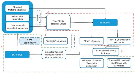
Figure 1.
Scheme for the analysis of the assimilation efficiency of the EnKF-SAFY_swb method. (1) Phase 1: Input setting. (2) Phase 2: “True” values evaluation. (3) Phase 3: “Synthetic” LAI values elaboration. (4) Phase 4: Model running. (5) Phase 5: Calculation of AE indicators.
In phase 2 (upper part of Figure 1), the SAFY_swb model is run using the “true” inputs and the meteorological data in order to obtain the “true” outputs, i.e., the values of LAI, ET, biomass and yield used as reference for the validation.
In Phase 3, the algorithm generates the “synthetic” LAI values, a simulation of LAI measurements estimated by EO data. They are generated adding an error to the “true” LAI.
During phase 4, the SAFY_swb model was run twice for each field, with and without assimilation, in order to obtain the biophysical variables for both cases and to compare them with the “true” values. The independent parameters to run the model are initially set in both cases using a generic calibration retrieved from the literature [13,21,47,48,49,50]. The initial values of parameters are reported in Supplementary Materials.
In phase 5 the simulated values of biophysical variables, in the presence of assimilation, and simulated values of biophysical variables without the assimilation are compared with the “true” values following the method proposed by [38] for calculating the Assimilation Efficiency Index (AE), as detailed here below.
First of all, the relative mean absolute errors (RMAE) were calculated, both for the method with assimilation () and for the method without assimilation (, as indicated in Equations (2) and (3), respectively:
where:
: number of fields (i.e., number of hypothetic scenarios);
: “true” value of Reference Biophysical variable (e.g., yield);
: simulated value of Reference Biophysical variable calculated using the assimilation method;
: simulated value of Reference Biophysical variable calculated running the crop model without the assimilation method.
Subsequently, the AE was calculated following Equation (4):
Equations (2)–(4) were proposed by [38].
2.2.1. General Case
We have defined the General Case as the application of the methodology proposed by [38] which aims to evaluate how the variation in the number of observations assimilated and the measurement error of the variable to be assimilated (in this case the LAI) affect the assimilation efficiency of EnKF-SAFY_swb.
The LAI to be assimilated ( is obtained by adding an error proportional to the same value to the “true” value of LAI, as shown in Equation (5):
where:
: day of assimilation;
: “true” value of LAI;
: coefficient of LAI error on the measurements;
considered in the general case are: 0.05, 0.1, 0.15, 0.2, 0.25, 0.3.
In this case, the number of assimilated observations was also varied. A set of 5, 10, 15 and 20 observations (and corresponding assimilations) were considered. In this way, 600 simulations were finally carried out. For the general case, the yield was used as a reference variable to calculate , and, consequently, the assimilation efficiency index (Equations (2)–(4)).
2.2.2. Specific Case
The specific case was analysed to obtain the assimilation efficiency for conditions very similar to the real case of study used to validate the EnKF-SAFY_swb method. The number of assimilated observations is fixed to 6 because this is the minimum number of Sentinel-2 images available for the area of interest during the crop growth cycle. The error of LAI measurement is fixed to 20%, as indicated in literature [44] for LAI derived from Sentinel-2 data using the SNAP software. Since the number of observations and the error on LAI are fixed, the number of simulations is equal to the number of fields, so it was possible to increase the number of fields in order to obtain a wider variety of potential scenarios. In this case, the number of fields has been set to 1000 for each initial scenario, for a total of 5000 simulations.
2.3. Grosseto Case Study (Central Italy)
All data acquired in situ used for the validation of this study were collected during the 2018 SurfSense campaign funded by ESA [51]. The field campaign was part of a larger activity in the context of future EO programmes promoted by Copernicus, the European Union’s Earth Observation Programme [6]. Specifically, the campaign described by [51] aims to demonstrate the validity of the Copernicus Candidate mission High Spatio-Temporal Resolution Land Surface Temperature Monitoring (LSTM). The LSTM mission aims to address water, agriculture and food security issues by monitoring the variability in LST (and hence evapotranspiration) at the European field scale enabling more robust estimates of field-scale water productivity [51]. LST is closely linked to ET, the reference variable chosen in this study to demonstrate the effectiveness of the EnKF-SAFY_swb method. Although the field campaign was not specifically designed for the presented study, the recorded data are very useful for the presented analysis.
2.3.1. Study Area and In Situ Data
The study area is in a farm (Le Rogaie) located in central Italy, in the province of Grosseto, in the coastal zone of Southern Tuscany (Figure 2). It is characterized by a Mediterranean climate, with very mild and wet winters and very hot summers. During winter, minimum temperatures during the night under 0 °C are common as well as maximum temperatures over 30 °C during the days of summer. Detailed climatic data of 2018 are shown in Figure 3. Consorzio Lamma, Laboratory of Meteorology and Environmental Modelling have provided temperatures, precipitation and daily solar radiation data. The meteorological station was located at 42.769 N and 11.016 E.
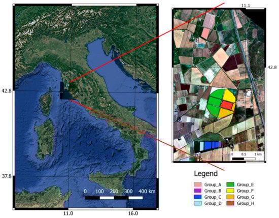
Figure 2.
Study area: Le Rogaie, Grosseto, Tuscany (Italy). The base map used for the image on the left was downloaded from the Google catalogue made available for the QGIS plugin QuickMapService. The base map used for the image on the right is a true color composite based on HyPlant raw data recorded on 20 July 2018 during SurfSense 2018 [51].
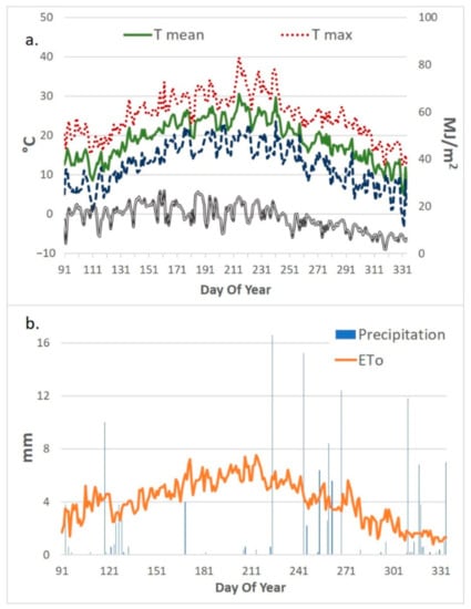
Figure 3.
Climatic data for Grosseto2018. (a) temperature and daily solar radiation; (b) precipitation and reference evapotranspiration. Data provided by Consorzio Lamma, Laboratory for Meteorology and Environmental Modelling.
Since data of daily solar radiation were not available for some days, the RadEst model [52] was applied to estimate the parameter for the missing days and fill the gaps. The reference evapotranspiration has been calculated using the FAO software ET0 Calculator [43].
The study area was limited to 13 fields, with a total area of 105 ha, all cultivated with maize in the period between April and September 2018. These fields were classified into 8 groups (from A to H) according to similar characteristics such as sowing date, management of irrigation and average trend of the LAI (Figure 2). The fields belonging to the groups A (in the northern part), B, C and D (in the southern part) were managed using fixed sprinkler irrigation systems during the maize growth period. The fields belonging to the groups D, E, F, G, H located within a circular area with a diameter of about one km were irrigated by a rotating pivot system, which is normally operated 24 h a day in the period June–August.
Details of the soil properties, obtained from an intensive sampling campaign carried out during summer 2018 in the study area are reported in Table 1.

Table 1.
Summary of soil property statistics of the study site (Grosseto, Central Italy).
A full irrigation cycle is completed within four days. A malfunction of the system did not allow proper irrigation between the 16th and 22nd of July.
Turbulent flux data were acquired using an Eddy-covariance (EC) system installed inside the pivot area (11.07073, 42.83203) in accordance to the EuroFlux methodology [53] the EC system was operational between the 143rd and 241st day of the year 2018 (23 May–29 August). The fluxes, including the latent heat flux data in W/m−2 used in this study, were calculated on half hourly intervals using the ECpack software [54]. The duration of the in situ measurement campaign coincides with the acquisition period of the EC system, while the meteorological data were acquired between September 2017 and September 2018.
2.3.2. Airborne Measurements
The airborne data used in this study were gathered as part of the Surfsense2018 ESA campaign and used to evaluate the ET [51]. The sensor used was the Thermal Airborne Spectrographic Imager (TASI-600), a push broom hyperspectral thermal sensor system specifically designed for airborne data acquisition. It is sensitive to wavelengths in the long wave infrared (LWIR) and measures the intensity of emitted radiance from the imaged target across 32 spectral bands in the range of 8 to 11.5 µm. The data were acquired on the 199th and 201st day of the year (18 and 20 July), between 12:00 p.m. and 4:00 p.m. (local time), following the flight plan shown in Figure 4. The data acquired with the TASI were used to estimate the Surface Temperature ().
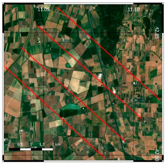
Figure 4.
Airborne flight plan used to record airborne data with the TASI-600 and HyPlant DUAL sensor. Airborne raw data were recorded during the 2018 Surfsense campaign [51]. The basemap was elaborated from Sentinel-2A data acquired on 8 July 2018.
Simultaneously, optically reflective data were acquired using the HyPlant DUAL airborne imaging spectrometer. HyPlant DUAL consists of two push-broom hyperspectral line scanners, which provide contiguous spectral information from 370 nm to 2500 nm with 3 nm spectral resolution in the VIS/NIR and 10 nm spectral resolution in the SWIR spectral range.
Both the data acquired with the TASI and HyPlant were processed during the Surfsense2018 campaign [51] to obtain the estimations of the instantaneous Latent Heat Flux (LE). These estimations were carried out using the Simplified Surface Energy Balance Index (S-SEBI) model described in [32,33].
All the details about the airborne acquired data and their processing to obtain the instantaneous LE are explained in detail in [51]. Further details are also provided in Supplementary Materials.
2.3.3. From Instantaneous LE to Daily Actual ET
In this study, we used two information sources for the ET estimation since the in situ estimates allowed a good monitoring over time, but, in a limited number of points on the ground, while the estimates made through airborne allowed a good spatial monitoring but for only two dates. In order to compare the daily ET simulated by the EnKF-SAFY_swb with the in situ and airborne estimates, it was necessary to convert the instantaneous LE () to daily actual Evapotranspiration (. For the EC data, the daily latent heat flux () was calculated by simply integrating the half hourly latent heat flux ( during the period of daylight using as time interval dt = 30 min. For the estimates of obtained from the airborne data, it was necessary to use a model that related to .
With a view to developing a methodology that can be adapted in the future to the use of daily land surface temperature data acquired via satellite (for example LSTM), it was decided to use a single estimate of to derive the daily ET. The methodology used to obtain this conversion is the one proposed by [55,56]. Further details are provided in Supplementary Materials.
2.3.4. Satellite Data
A set of nine Level 2 cloud free Sentinel 2 images covering the study area was selected for the analysis. The level 2 images were processed with the SNAP module S2toolbox [44] to estimate the LAI (Table 2).
Table 2.
List of Sentinel-2 Level 2 images used for this study and their day of acquisition (column 2). In the column called Validation, the images classified as “no” were used for the assimilation, while the images classified with capital letters were used to validate the results of the group of fields corresponding to the latter.
The trend of average LAI for each group of fields (defined as described in Section 2.3.1) and the corresponding standard deviation were calculated and are shown in Figure 5. For each trend, the images were used for the assimilation, except the last image of the trend, which was used to validate the simulations generated with the EnKF-SAFY_swb.
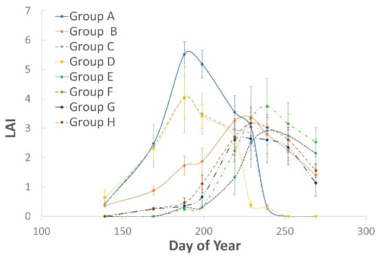
Figure 5.
Average LAI Trend estimated from Sentinel-2 data. The error bars represent the standard deviation for each group of fields.
The study area analysis was conducted for each group of fields, which are characterized by different LAI trends. Therefore, the number of observations monitoring the trend of LAI varies for each group. It is composed of the number of assimilated images (specified in Table 3), plus one image (the last available for each cultural cycle that characterizes the group) used for validation. The number of images used in the proposed assimilation method varies from a minimum of 6 to a maximum of 8, depending on the group of fields under examination. On the other hand, a single image was used to validate the performance of the model in simulating the LAI trend. Some previous studies, e.g., refs. [13,57], have shown that it is possible to improve the performance of a crop growth model by using an assimilation method for updating, even using a small number of images. Therefore, the number of assimilations used in this study is sufficient to allow the application of the proposed assimilation method.
Table 3.
List of groups of fields. Each group has the same sowing date, harvest date and number of available LAI observations.
2.3.5. EnKF-SAFY_swb Method Pre-Processing
As mentioned in Section 2.1.2, the majority of parameters of the model are kept constant during the run of EnKF-SAFY_swb (Table 4 and Table 5), while 5 parameters are varied during the model runs (Table 6).
Table 4.
List of model fixed parameters and their calibration values.
Table 5.
Soil parameters, calibrated by crossing [51,50]. They were kept constant during EnKF-SAFY_swb run.
Table 6.
List of parameters that vary in EnKF-SAFY_swb.
The parameters of the model kept constant during the run of SAFY_swb are shown in Table 4 and Table 5. They are calibrated using information obtained in situ, from airborne data and EO data [51] and information retrieved by literature [21,47,49,50,58]. The calibration is intentionally generic because the idea is to test the efficiency of the EnKF-SAFY_swb methodology in the absence of a specific calibration for each field which is generally a great difficulty in using crop growth models.
The parameters to be changed during the execution of EnKF-SAFY_swb were chosen based on the sensitivity analysis made by [59]. To simplify the computational process of the algorithm, only the five parameters that most affect the model were selected to be varied.
As suggested by literature [13,45,60,61], the size N of the ensemble used in the EnKF DA method (N corresponds to the number of simulations for each pixel) has to be big enough to ensure the convergence of the model [46]. For this study, N was set to 200 [13]. The error of the model is considered as a percentage of the mean simulated LAI and is set to 20% [13], as suggested by the results obtained evaluating the assimilation efficiency of the developed methodology (Section 2.2). The error of the measurement was set at 20% as described by [51].
3. Results
3.1. Assimilation Efficiency
The assimilation efficiency analysis studied in the “Generic Case” (Section 2.2.1) is summarized in Figure 6 and Figure 7. In particular, Figure 6a shows the comparison between the LAI considered “true” with the LAI simulated by the model without using the assimilation. The LAI considered “true” is the value of LAI obtained in the first run of the model with the synthetic dataset and the “real” parameters (for details, see Section 2.2). The LAI simulated is the LAI obtained in the second run of the model, using a generic calibration of the parameters, the same synthetic data previously used to obtain the “true value”. In this case, the RMSE (between “true” and “simulated values) is 0.70, the RRMSE is around 41% and the coefficient of determination (R2) is 0.9. The comparison with the LAI simulated coupling SAFY_swb with the EnKF DA method (Figure 6b) shows a clear improvement brought about by the assimilation. The resulting RMSE is 0.48, the RRMSE is around 28% and R2 is of 0.94.
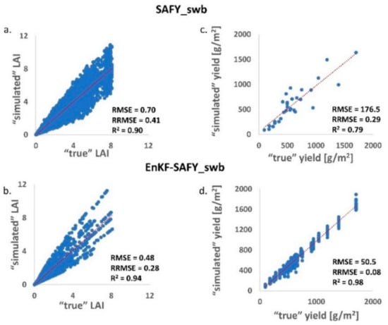
Figure 6.
Comparison between “true” and “simulated” variables (generated with and without assimilation) for a synthetic dataset (generated following the procedure described in Section 2.2. (a) Comparison and linear regression between “true” LAI and “simulated” LAI generated without assimilation (using the SAFY_swb crop growth model); (b) comparison and linear regression between “true” LAI and “simulated” LAI generated with assimilation (using the methodology EnKF-SAFY_swb); (c) comparison and linear regression between “true” yield and “simulated” yield generated without assimilation (SAFY_swb); (d) comparison and linear regression between “true” yield and “simulated” yield generated with assimilation (EnKF-SAFY_swb). For each case RMSE, relative RMSE (RRMSE) and coefficient of determination (R2) are shown.
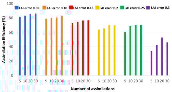
Figure 7.
Assimilation efficiency index calculated with synthetic data as described in Section 2.2. Each column represents a different number of assimilations (the value is reported on the x-axis) while each colour represents a different error on “measured” LAI. For simplicity of calculation, AE is valued against yield.
A comparison between “true” and “simulated” value is shown also for the yield. In Figure 6c, the “true” yield (estimated similarly to the LAI) is compared with the “yield” simulated by SAFY_swb open loop. The RMSE is of 176.5 , the RRMSE is estimated around the 29% and the R2 is of 0.79. Applying the assimilation (Figure 6d), the RMSE was distinctly reduced to 50.5 , with an RRMSE of around 8% and an R2 of 0.98.
In Figure 7, the assimilation efficiency index calculated for each combination (number of assimilated observations and error of LAI) is shown. Each column represents a different number of assimilated observations (indicated on the horizontal axis) while each colour represents a different value of error on the “measurement” of LAI. As the error increases, the assimilation efficiency decreases markedly. The increase in the number of assimilated observations determines an improvement, albeit small and, in some cases, negligible in terms of efficiency.
In Figure 8, the results of assimilation efficiency analysis for the specific case (the characteristics of this case are detailed in Section 2.2.2) are shown. Figure shows the comparison between the simulated LAI using EnKF-SAFY_swb and the “true” value of LAI obtained from synthetic data. For the LAI, the RMSE is 0.50 (which corresponds to an RRMSE of about 21%). In Figure 8B, the results for actual evapotranspiration (expressed in mm) are shown. In this case, the RRMSE is of around 18%. In Figure 8C, the comparison between the simulated biomass using EnKF-SAFY_swb and the “true” biomass obtained from synthetic data is shown. For the biomass, the RRMSE turned out to be around of 16%. Finally, in Figure 8D, the effect of assimilation on yield estimation is presented. This analysis shows that the EnKF assimilation method combined with the SAFY_swb model is able to estimate (for a synthetic dataset) the yield with an error of about 11%.
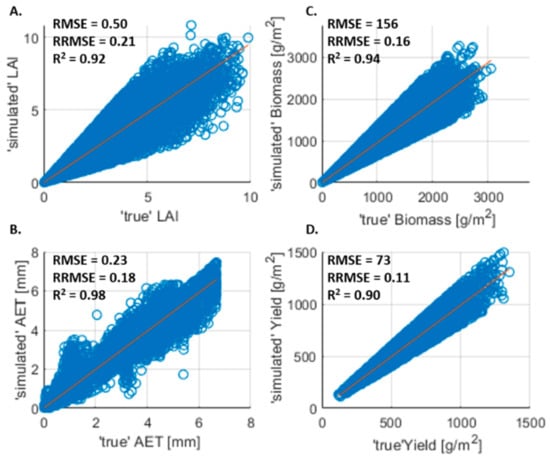
Figure 8.
Comparison of “true” and “simulated” variable obtained using the EnKF-SAFY_swb data assimilation method for a synthetic dataset (6 assimilated observations). A set of 5000 simulations is used. For each variable RMSE, relative RMSE and R2 are shown. In detail: (A) comparison and linear regression between “true” and “simulated” LAI; (B) comparison and linear regression between “true” and “simulated” actual evapotranspiration; (C) comparison and linear regression between “true” and “simulated” biomass (expressed in ; (D) comparison and linear regression between “true” and “simulated” yield (expressed in ).
In the specific case, the AE index (as described in Section 2.2) was calculated with respect to yield and actual ET (AET). The AE with respect to yield was estimated at around 63%. This value is consistent with the result achieved in the generic case when the error on LAI was 20%, and the number of assimilations was set to 5. The AE with respect to AET was estimated at around 67%.
3.2. Grosseto Case Study (Central Italy)
To evaluate the agreement between the latent heat flux measurements acquired in situ from Eddy Covariance measurements (Section 2.3.1) and the estimates derived by combining the airborne data recorded by TASI and HyPlant (Section 2.3.2), data acquired on the same date (days of year 199th and 201st) have been compared (Figure 9). A polynomial regression of 6th degree was calculated for the EC data. Then, the values of the polynomial regression at the time of airborne data acquisition were compared with the LE estimated from the airborne data. The resulting overall (for both dates) RMSE was 20.06 and the RRMSE had a value of about 9%.
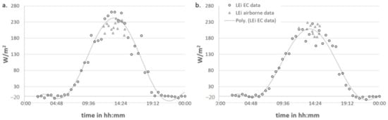
Figure 9.
Comparison of latent heat flux (LEi) measured with Eddy Covariance (circle) and calculated from airborne data (triangle), for the 199th (a) and 201st DOY (b). The line represents a polynomial regression function (6 degree) fitted through the LEi measurements from the EC station.
Starting from the LEi measured in situ and the LE estimated from airborne data, the daily AET was calculated as described in Section 2.3.3 and compared with the AET simulated by EnKF-SAFY_swb (Figure 10). The measurements estimated from airborne data were available only in two dates, i.e., not enough for an accurate representation of the temporal trend of AET. In fact, these data were used for a spatial representation of the AET (which is not possible with the EC measurements). In Figure 10, the airborne data were plotted only to have a qualitative comparison. The RMSE between the daily actual evapotranspiration observed in situ from EC and that one simulated by ENKF-SAFY_swb is of 0.8 mm, the RRMSE is around 27% and the coefficient of determination is of 0.46.
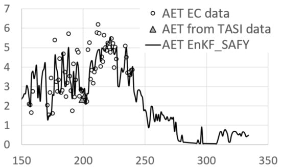
Figure 10.
Comparison between dailyactual evapotranspiration (AET) measured with EC (circles), calculated from airborne data (triangles) and simulated with EnKF-SAFY_swb (continuous line).
Subsequently, the method EnKF-SAFY_SWB was applied to generate AET maps for the 199th and 201st day of the year. Those maps were subsequently compared with the AET maps obtained from the airborne data. Figure 11 shows the scatter plot of the comparison of both maps. In this case, the RMSE is 0.55 mm, the RRMSE is around 27% and the coefficient of determination (R2) is 0.76.
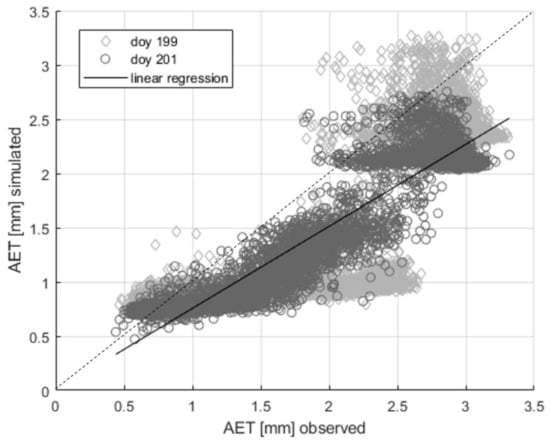
Figure 11.
Comparison between AET calculated using airborne data (horizontal axis) and simulated using EnKF-SAFYswb (vertical axis), for the day of year (DOY) 199 (diamonds) and 201 (circles). The dashed line is the 1:1 simulated vs. the observed line.
In Figure 11, a clear 2 clusters separation can be noted. This is the result of differences in fractional cover between the fields forming the various groups (for those dates) as it can be deducted from the differences in S2 derived LAI (Figure 5) from the DOY 200 (19th of July). This shows the model’s capability to estimate AET sufficiently reliable for various vegetation fractional covers.
In Table 7, the RMSE and RRMSE of each group of fields are shown. The RRMSE varies between a minimum of 20% to a maximum of 43%.
Table 7.
Root Mean Square Error (RMSE) and Relative RMSE (RRMSE) calculated for each group of fields (as defined in Section 2.3.1) comparing the actual evapotranspiration (AET) calculated from airborne data (both images) and AET simulated by EnKF-SAFY_swb.
By comparing the daily AET maps obtained from airborne data (upper part of Figure 12) with those simulated by the EnKF-SAFY_swb method (lower part of Figure 12), it can be seen that the simulations tend to be underestimated, especially in the pivot zones classified as Group G and Group H (lower right of the pivot).
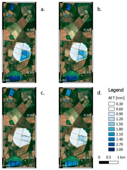
Figure 12.
(a) Map of daily Actual ET (mm) for the DOY 199 estimated using airborne data. (b) map of Actual ET (in mm) for the DOY 201 estimated using airborne data; (c) map of Actual ET for the DOY 199simulated using EnKF-SAFY_swb; (d) map of Actual ET for the DOY 201simulated using EnKF-SAFY_swb.
This underestimation effect is even clearer when looking at the histograms of the ET calculated from airborne data and that estimated with EnKF-SAFY_swb (Figure 13). In fact, comparing the bins of the two histograms, it is possible to note that for the images simulated by EnKF-SAFY_swb. The bins of the points between 0.7 and 0.9 mm are double the corresponding bins of the images elaborated from airborne data, while the bins between 1.5 and 2 mm are almost zero in the case of data simulated by the model. Furthermore, the point peak between 2.7 and 3 mm in the case of the elaborations made by airborne data is shifted to the interval 2–2.5 mm in the case of the ET simulated by EnKF-SAFY_swb.
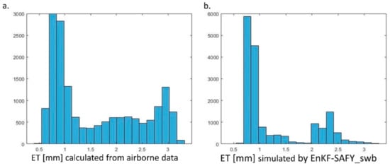
Figure 13.
(a) Histogram of daily ET (expressed in mm) calculated from airborne data; (b) histogram of daily ET (expressed in mm) simulated by EnKF-SAFY_swb.
We also validated the LAI simulations generated with EnKF-SAFY_swb. In this case, the observed data were estimated from Sentinel-2 data. In Figure 14, the comparison for each group is shown, while Table 8 provides the corresponding RMSE and RRMSE values.
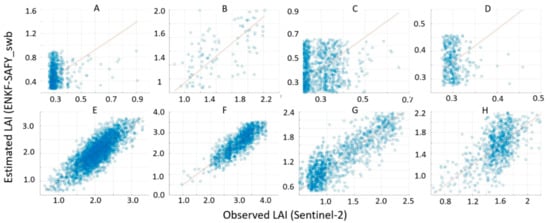
Figure 14.
Comparison and linear regression between LAI estimated from Sentinel-2 data (horizontal axes) and LAI simulated by EnKF-SAFY_swb (vertical axis) for each group of fields (as classified in Section 2.3.1, each letter corresponds to a group of fields). (A) Group A; (B) Group B; (C) Group C; (D) Group D; (E) Group E; (F) Group F; (G) Group G; (H) Group H.
Table 8.
Root Square Mean Error (RMSE) and Relative RMSE (RRMSE) calculated for each group of fields (as defined in Section 2.3.1) comparing the Leaf Area Index (LAI) calculated from Sentinel-2 data and LAI simulated by EnKF-SAFY_swb.
The LAI simulated with EnKF-SAFY and estimated by Sentinel-2 data for the entire area covered by the studied fieldswere compared in Figure 15, obtaining an RMSE of 0.27, an RRMSE of around 18% and a R2 of 0.9.
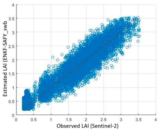
Figure 15.
Comparison and linear regression between LAI estimated from Sentinel-2 data (horizontal axes, denominated as obs) and LAI simulated by EnKF-SAFY_swb (vertical axis, denominated as sim) for the whole area of study.
4. Discussion
One of the aims of this paper was to study the validity of the proposed DA method based on the EnKF coupled with the new model SAFY_swb. More specifically, we aimed at evaluating if the EnKF-SAFY_swb method would be more effective than the simple SAFY_swb model in simulating the crop growth. Furthermore, we wanted to understand how much the assimilation efficiency depends on the number of assimilations and on the error on the variable to be assimilated.
The “general case” (Section 2.2.1) was useful in defining the relationship between the number of assimilations and the efficiency of the method, and it also made it possible to establish the LAI error limit value for which the use of this assimilation method is convenient. For this case, the AE is evaluated only with respect to yield, since it is the variable of greatest interest in a crop growth model. The “specific case” (Section 2.2.2), on the other hand, made it possible to quantify in a more decisive way (allows to use a large number of input scenarios) the usefulness of using the EnKF assimilation method with the SAFY_swb model.
The results of the AE analysis for the “general case” highlight that the use of the EnKF DA method on SAFY_swb led to an improvement in accuracy both in estimating LAI and yield (Figure 6). Particularly surprising is the reduction in RMSE for yield, which is estimated using the EnKF. RMSE distinctly decreased from 176.5 to 50.5 . This result, although encouraging, cannot be considered fully reliable, as the dataset is generated with a small number of “true” cases. The number of scenarios considered is not sufficient to unequivocally define the AE of the EnKF-SAFY_swb method.
The analysis for the general case is, on the other hand, very useful to quantify the influence of the number of observations to be assimilated and of the acceptable error of the observed variable (i.e., the LAI) on the AE of the method. From this analysis, it resulted in the fact that the error on the LAI measurements greatly influences the AE (Figure 7). In particular, the use of the assimilation method is very suitable for LAI errors between 0.05 and 0.1, suitable for estimation errors on the LAI of 0.15, sufficiently suitable for errors between 0.2 and 0.25. For measurement errors exceeding 0.25, the assimilation method, compared to the use of the simple model, is no longer beneficial. It is therefore possible to establish an estimation error in LAI of 0.25 as a threshold value obtaining better results when using the DA technique. The number of assimilated observations, therefore, does not significantly affect the AE, especially for low LAI errors. The influence of the LAI starts to become relevant for errors higher than 0.2. In the case of LAI estimations from Sentinel-2 data, the error on the LAI is around 0.2, and thus the use of EnKF-SAFY_swb has proven to be useful to improve the crop variable estimations. The AE relative to the yield evaluated for five assimilation dates and for an LAI error of 0.2 (i.e., a case similar to the “specific case” and to the real case study) is slightly above 60%.
Once the estimation error limit of the LAI and the minimum number of assimilations had been established, it was possible to analyse the assimilation efficiency of the EnKF-SAFY_swb method. The database generated in the specific case adopted a number of assimilated observations and error on LAI observations similar to those found in the case study. In this way, it was possible to generate a dataset large enough to rigorously establish the assimilation efficiency of the proposed method. In this case, the comparisons between “true” and “simulated” variables were shown not only for LAI and production but also for biomass and actual evapotranspiration (Figure 8). Both parameters give an idea of the model’s potential (useful to inspire future studies) and, in the real case analysed, the focus was mainly on the estimation of AET. This is why the AE was calculated both for yield and AET.
The error on the yield is slightly higher than in the general case, albeit with a value that justifies the use of the assimilation method. We can therefore state that, for a number of assimilated observations higher than 5 and an LAI error lower than 0.2, the yield estimation error is at least 11% (value obtained using a synthetic dataset), and the AE with respect to the yield of using the EnKF-SAFY_swb method is estimated at around 63%. This value agrees with the value of AE evaluated in the “general case” for five assimilated observations and an LAI error of 0.2.
For the AET, the estimation error (RMSE) is about 0.23 mm (equal to the 18% of the average measurement). In this case, the AE is approximately 67%, a value that indicates how sufficiently useful it is to increase the estimates made by the SAFY_swb crop growth model with the EnKF assimilation method. It should be noted that this cannot be considered a proper validation, but it is rather the step prior to a use “on-the-field”. On the one hand, it proves the correctness of the theoretical principles on which the method is based on (and its correct application). On the other hand, it provides a reference system that any “real” case study can be compared with.
The validation of the assimilation method based on the Kalman Filter Ensemble applied to the SAFY_swb crop growth model proposed in this study was applied to a data set recorded in central Italy in 2018 (case study, Section 2.3).
We extrapolated from the images acquired via airborne the points corresponding to the geographical position of the EC footprint. We compared the daily trend of LEi in the days of acquisition via airborne in the interval of time in which the flight took place. This is a purely qualitative comparison because of the relatively small data set. This comparison (Figure 9) shows that there is correspondence between the data with an average error of 9% (between the airborne and the EC measurements). In this specific case, we are interested in analysing the ET, which, according to the method suggested by [55] and described in Section 2.3.3, is calculated using a single measure of daily LEi. The comparison in Figure 9 therefore allowed to select the time in which the estimation of LEi derived from the airborne data is closer to the maximum of the polynomial regression function calculated from the LEi estimations measured by the EC sensor.
Concerning the validation of the method’s ability to simulate the ET trend, the comparison with the data measured in situ shows a low correspondence (a R2 of around 0.46 and an RRMSE of around 27%), especially in the period between the days 195th (14 July) and 207th (5 August) (Figure 10).This error could be attributed to the inaccuracy of the climatic input data. The weather station was not exactly located in the study area, but a few kilometres south of it. For a field-scale study, this distance can introduce a non-negligible error. Another reason could be an incorrect calibration of the parameters of the SAFY_swb model, and further experiments are needed to confirm or disprove these hypotheses.
Regarding the application of the EnKF-SAFY_swb method for the simulation of daily ET maps for a predetermined date, the validation showed a fair correspondence. The relative RMSE between the ET processing obtained from the airborne data and the ET simulated by the model is approximately 27%. Considering that the error on the initial LAI was set at 20%, the relative RMSE obtained can be considered a satisfactory result. However, it highlights that the assimilation of remotely sensed data brings an improvement to the model. Analysing the individual groups of fields in detail, it is noted that the RRMSE is around 20% for six groups out of eight and around 40% for the remaining 2. Both groups of fields with a relatively high RRMSE are part of the pivot, the area for which a malfunction of the irrigation system was reported (preventing the precise knowledge of the quantity of water administered). This drawback has forced approximations on some input parameters considered fixed during the assimilation (such as the amount of water used for irrigation), which could be partly caused due to errors on the initial calibration of the parameters. This is very evident by observing the daily ET maps proposed in Figure 12. The histograms of those images (Figure 13) highlight a difficulty of the method in simulating the variations of ET, tending to assume the most frequent values. They also confirm a tendency of the model to underestimate the ET, particularly in some fields within the pivot.
However, even if the expectations given by the results obtained using the synthetic dataset (an RRMSE of about 18%) were higher, the results obtained from real data are sufficiently valid, even if they leave many possibilities for improvement of the proposed methodology.
For the sake of completeness, a validation was also carried out on the LAI, using as reference measures the LAI values processed starting from Sentinel-2 data, not used in assimilation. It was decided to always use the latest available date of the crop cycle of each group of fields. Analysing the RRMSE group-by-group (Figure 14 and Table 8), the method is very accurate in 6 out of 8 cases and not valid in the remaining 2. Both groups of fields for which the RRMSE is very high have LAI values on average lower than 1, and this suggests a difficulty of the methodology in simulating the LAI for low values in the final phase of the cultural cycle. The absolute RMSE in fact is not discordant with that of the other fields; the relative one, however, referring to small values of LAI, is very high. Analysing instead the entire area covered by the studied fields, the results are consistent with what was found using synthetic data.
Analysing the literature, some common problems emerged in the synergistic use of EO data with crop models through DA methods. The problem of parameter calibration was solved with in situ measurements, in order to reduce the number of parameters with high uncertainty to 5 (parameters varied in the application of the DA method). This solution is not optimal for the use of low cost and low environmental impact methods; it is therefore necessary to implement tools capable of acquiring data remotely. The difficulty in having high spatial resolution and high temporal frequency for the method validation data has been circumvented by using synthetic datasets. This is a preliminary check, to be confirmed by field applications, but, in any case, allows highlighting the strengths and weaknesses of the methodology, thus suggesting possible improvements. The choice of two synthetic datasets (above defined as “general case” and “specific case”) was necessary to solve the problem of too high computation time (already found in other previous studies, such as [13,62,63]). Dividing it into two steps, the processing times were reduced and an analysis on some EnKF DA typical parameters was also provided: the number of assimilations and the threshold error on the assimilated data. In the real case, however, the problem of having high spatial resolution data for validation was addressed using images acquired from aircraft, while daily (punctual) data were used to solve the problem related to the high temporal frequency. This strategy allows for a preliminary validation with real data, which further confirm the benefits that satellite missions such as LSTM, which aims to provide high-resolution, high-frequency ET maps.
5. Conclusions
The method proposed in this study, which uses the LAI retrieved from Sentinel-2 data with a modified version of SAFY that considers the soil water balance as an input, through a DA method based on the EnKF, sought to address some of the most common problems found in the literature. We studied the problem both from a spatial and temporal point of view. It is part of the scientific field of DA methods for a synergistic use of EO data with crop growth model that uses a filtering approach, according to the classification proposed by [2].
The study aims to propose a methodology that allows future practical applications at field scale, thus providing information that in addition to detailing the growth of crops is also useful to optimize water resources. Precisely for this reason, we have chosen to use a model such as SAFY_swb, capable of simulating the evolution of ET over time and its implications for the development of the crop.
The main limitations of this study are:
- -
- Few acquisitions of satellite images from which to obtain the LAI for the updating of the model.
- -
- Few images acquired via airborne for validation
- -
- Single Eddy Covariance tower on the ground
- -
- Lack of an active in situ weather station for the entire crop cycle.
The proposed methodology was developed considering these limitations and trying, as far as possible, to reduce their effects on the results.
In conclusion, it can be stated that the EnKF-based DA method has been shown to be valid for the SAFY_swb crop growth model, confirming good results in the simulation of biomass and yield (to be validated also in real cases) and equally good ability in monitoring LAI and ET. The first can be improved by increasing the number of assimilations, the second, albeit valid in providing an overall trend of the data, to be improved especially in the accuracy of the daily data. In addition, the model has proven to address ET’s daily requirements by efficiently assimilating the EO data.
A good calibration continues to be essential to use crop models, which cannot always be solved efficiently with in situ measurements. It has further been shown, through the use of synthetic data, that the lack of good calibration could be partially avoided by increasing the number of assimilations. However, results improved in a much more significant way by increasing the accuracy of the assimilated variable. The studies conducted so far suggest that assimilating multiple variables simultaneously (with the highest temporal frequency and spatial resolution possible) could further compensate for the impossibility of calibrating the parameters that can be measured mainly in situ. Another possible improvement for future studies would be the use of specific meteorological data recorded in a study site, so that the elaborated maps can further consider the variability on the area under study.
Supplementary Materials
The following are available online at https://www.mdpi.com/article/10.3390/rs13112138/s1, Document S1: Supplementary material.docx.
Author Contributions
Conceptualization, P.C.S. and R.C.; methodology, P.C.S. and R.C.; software, P.C.S.; validation, P.C.S., D.S. (Drazen Skokovic) and J.S.; formal analysis, P.C.S.; investigation, P.C.S.; resources, P.C.S., J.H., B.K., U.R. and D.S. (Dirk Schuettemeyer), B.S., D.S. (Drazen Skokovic), J.S. and M.T.; data curation, P.C.S., J.H., B.K., U.R. and D.S. (Dirk Schuettemeyer), B.S., D.S. (Drazen Skokovic), J.S. and M.T.; writing—original draft preparation, P.C.S.; writing—review and editing, P.C.S., R.C., B.K., B.S. and M.T.; visualization, P.C.S. and B.S.; supervision, B.K.; project administration, P.C.S. All authors have read and agreed to the published version of the manuscript.
Funding
This research received no external funding.
Institutional Review Board Statement
Not applicable.
Informed Consent Statement
Not applicable.
Data Availability Statement
The satellite data used in this study (Sentinel-2 data) are freely accessible via the Copernicus Open Access Hub (https://scihub.copernicus.eu/, accessed on 1 June 2020). The data concerning the climatic conditions are accessible on request at the Lamma Consortium, Laboratory of Meteorology and Environmental Modelling (info@lamma.toscana.it, provided on 12 May 2020). The data relating to the SurfSense 2018 measurement campaign are stored in ESA servers and available on request. All the above data used in this study are available upon request to the authors (paolo.cosmo.silvestro@esa.int).
Acknowledgments
The authors would like to express its gratitude to all the scientists, professionals, and participants at the SurfSense 2018, technical assistance for airborne and ground measurements during the high spatio-temporal resolution Land Surface Temperature Experiment, and the measurement campaign that provided almost all of the data used to validate the methodology proposed in this study. Thanks are also due to Consorzio Lamma, Laboratory of Meteorology and Environmental Modelling, which provided meteorological data used in this study. The authors would also like to thank to Emma Segovia for her help in correcting the spelling and grammar of the text.
Conflicts of Interest
The authors declare no conflict of interest.
References
- FAO. The Future of Food and Agriculture–Trends and Challenges; FAO: Rome, Italy, 2017; Available online: http://www.fao.org/3/i6583e/i6583e.pdf (accessed on 28 May 2021).
- Huang, J.; Gómez-dans, J.L.; Huang, H.; Ma, H.; Wu, Q.; Lewis, P.E.; Liang, S.; Chen, Z.; Xue, J.; Wu, Y.; et al. Agricultural and Forest Meteorology Assimilation of remote sensing into crop growth models: Current status and perspectives. Agric. For. Meteorol. 2019, 276–277, 107609. [Google Scholar] [CrossRef]
- Weiss, M.; Jacob, F.; Duveiller, G. Remote Sensing of Environment Remote sensing for agricultural applications: A meta-review. Remote Sens. Environ. 2020, 236, 111402. [Google Scholar] [CrossRef]
- Sishodia, R.P.; Ray, R.L. Applications of Remote Sensing in Precision Agriculture: A Review. Remote Sens. 2020, 12, 3136. [Google Scholar] [CrossRef]
- Huang, Y.; Chen, Z.; Yu, T.; Huang, X.; Gu, X. Agricultural remote sensing big data: Management and applications. J. Integr. Agric. 2018, 17, 1915–1931. [Google Scholar] [CrossRef]
- Jutz, S.; Milagro Perez, M.P. Copernicus space component: Status and evolution. In EGU General Assembly Conference Abstracts; EGU General Assembly Conference Abstracts; EGU: Wien, Austria, 2017; p. 18668. Available online: https://ui.adsabs.harvard.edu/abs/2017EGUGA..1918668J/abstract (accessed on 28 May 2021).
- Siad, S.M.; Iacobellis, V.; Zdruli, P.; Gioia, A.; Stavi, I.; Hoogenboom, G. A review of coupled hydrologic and crop growth models. Agric. Water Manag. 2019, 224, 105746. [Google Scholar] [CrossRef]
- Beveridge, L.; Whitfield, S.; Challinor, A. Crop modelling: Towards locally relevant and climate-informed adaptation. Clim. Chang. 2018, 147, 475–489. [Google Scholar] [CrossRef]
- Challinor, A.J.; Müller, C.; Asseng, S.; Deva, C.; Nicklin, K.J.; Wallach, D.; Vanuytrecht, E.; Whitfield, S.; Ramirez-Villegas, J.; Koehler, A.-K. Improving the use of crop models for risk assessment and climate change adaptation. Agric. Syst. 2018, 159, 296–306. [Google Scholar] [CrossRef]
- Biswal, A.; Chakraborty, A.; Murthy, C.S. Spatialization of Crop Growth Simulation Model Using Remote Sensing BT-Geospatial Technologies for Crops and Soils; Mitran, T., Meena, R.S., Chakraborty, A., Eds.; Springer: Singapore, 2021; pp. 153–199. [Google Scholar]
- Hoefsloot, P.; Ines, A.; van Dam, J.; Duveiller, G.; Kayitakire, N.F.; Hanse, J. Combining Crop Models and Remote Sensing for Yield Prediction: Concepts, Applications and Challenges for Heterogeneous, Smallholder Environments; European Union: Luxembourg, 2012; p. 52. [Google Scholar]
- Kasampalis, D.A.; Alexandridis, T.K.; Deva, C.; Challinor, A.; Moshou, D.; Zalidis, G. Contribution of Remote Sensing on Crop Models: A Review. J. Imaging 2018, 4, 52. [Google Scholar] [CrossRef]
- Silvestro, P.C.; Pignatti, S.; Pascucci, S.; Yang, H.; Li, Z.; Yang, G.; Huang, W.; Casa, R. Estimating Wheat Yield in China at the Field and District Scale from the Assimilation of Satellite Data into the Aquacrop and Simple Algorithm for Yield (SAFY) Models. Remote Sens. 2017, 9, 509. [Google Scholar] [CrossRef]
- Kang, Y.; Özdoğan, M. Field-level crop yield mapping with Landsat using a hierarchical data assimilation approach. Remote Sens. Environ. 2019, 228, 144–163. [Google Scholar] [CrossRef]
- Tewes, A.; Hoffmann, H.; Krauss, G.; Schäfer, F.; Kerkhoff, C.; Gaiser, T. New Approaches for the Assimilation of LAI Measurements into a Crop Model Ensemble to Improve Wheat Biomass Estimations. Agronomy 2020, 10, 446. [Google Scholar] [CrossRef]
- Li, Z.; Wang, J.; Xu, X.; Zhao, C.; Jin, X.; Yang, G.; Feng, H. Assimilation of Two Variables Derived from Hyperspectral Data into the DSSAT-CERES Model for Grain Yield and Quality Estimation. Remote Sens. 2015, 7, 12400–12418. [Google Scholar] [CrossRef]
- Jin, X.; Li, Z.; Yang, G.; Yang, H.; Feng, H.; Xu, X.; Wang, J. Winter wheat yield estimation based on multi-source medium resolution optical and radar imaging data and the AquaCrop model using the particle swarm optimization algorithm. ISPRS J. Photogramm. Remote Sens. 2017, 126, 24–37. [Google Scholar] [CrossRef]
- He, L.; Mostovoy, G. Cotton Yield Estimate Using Sentinel-2 Data and an Ecosystem Model over the Southern US. Remote Sens. 2019, 11, 2000. [Google Scholar] [CrossRef]
- Awad, M.M. An innovative intelligent system based on remote sensing and mathematical models for improving crop yield estimation. Inf. Process. Agric. 2019, 6, 316–325. [Google Scholar] [CrossRef]
- Monteith, J.L.; Moss, C.J. Climate and the Efficiency of Crop Production in Britain [and Discussion]. Philos. Trans. R. Soc. B Biol. Sci. 1977, 281, 277–294. [Google Scholar]
- Duchemin, B.; Maisongrande, P.; Boulet, G.; Benhadj, I. A simple algorithm for yield estimates: Evaluation for semi-arid irrigated winter wheat monitored with green leaf area index. Environ. Model. Softw. 2008, 23, 876–892. [Google Scholar] [CrossRef]
- Papadavid, G.; Toulios, L. The use of earth observation methods for estimating regional crop evapotranspiration and yield for water footprint accounting. J. Agric. Sci. 2018, 156, 599–617. [Google Scholar] [CrossRef]
- Tewes, A.; Hoffmann, H.; Nolte, M.; Krauss, G.; Schäfer, F.; Kerkhoff, C.; Gaiser, T. How Do Methods Assimilating Sentinel-2-Derived LAI Combined with Two Different Sources of Soil Input Data Affect the Crop Model-Based Estimation of Wheat Biomass at Sub-Field Level? Remote Sens. 2020, 12, 925. [Google Scholar] [CrossRef]
- Stancalie, G.; Marica, A.; Toulios, L. Using earth observation data and CROPWAT model to estimate the actual crop evapotranspiration. Phys. Chem. Earth Parts A/B/C 2010, 35, 25–30. [Google Scholar] [CrossRef]
- Petropoulos, G.P.; Srivastava, P.K.; Piles, M.; Pearson, S. Earth Observation-Based Operational Estimation of Soil Moisture and Evapotranspiration for Agricultural Crops in Support of Sustainable Water Management. Sustainability 2018, 10, 181. [Google Scholar] [CrossRef]
- Pelosi, A.; Villani, P.; Falanga Bolognesi, S.; Chirico, G.B.; D’Urso, G. Predicting Crop Evapotranspiration by Integrating Ground and Remote Sensors with Air Temperature Forecasts. Sensors 2020, 20, 1740. [Google Scholar] [CrossRef] [PubMed]
- Hartanto, I.M.; Van Der Kwast, J.; Alexandridis, T.K.; Almeida, W.; Song, Y. Data assimilation of satellite-based actual evapotranspiration in a distributed hydrological model of a controlled water system. Int. J. Appl. Earth Obs. Geoinf. 2017, 57, 123–135. [Google Scholar] [CrossRef]
- Koetz, B.; Bastiaanssen, W.; Berger, M.; Defourney, P.; Del Bello, U.; Drusch, M.; Drinkwater, M.; Duca, R.; Fernandez, V.; Ghent, D.; et al. High Spatio- Temporal Resolution Land Surface Temperature Mission—A Copernicus Candidate Mission in Support of Agricultural Monitoring. In Proceedings of the IGARSS 2018—2018 IEEE International Geoscience and Remote Sensing Symposium, Valencia, Spain, 22–27 July 2018; pp. 8160–8162. [Google Scholar]
- Mission Science Division. Copernicus High Spatio-Temporal Resolution Land Surface Temperature Mission: Mission Requirements Document; ESA: Noordwijk, The Netherlands, 2019; pp. 1–89. [Google Scholar]
- Lagouarde, J.-P.; Bhattacharya, B.K.; Crébassol, P.; Gamet, P.; Adlakha, D.; Murthy, C.S.; Singh, S.K.; Mishra, M.; Nigam, R.; Raju, P.V.; et al. Indo-french high-resolution thermal infrared space mission for earth natural resources assessment and monitoring–concept and definition of trishna. ISPRS-Int. Arch. Photogramm. Remote Sens. Spat. Inf. Sci. 2019, XLII-3/W6, 403–407. Available online: https://hal-normandie-univ.archives-ouvertes.fr/hal-02420462/document (accessed on 28 May 2021).
- Bastiaanssen, W.G.M.; Menenti, M.; Feddes, R.A.; Holtslag, A.A.M. A remote sensing surface energy balance algorithm for land (SEBAL). 1. Formulation. J. Hydrol. 1998, 212–213, 198–212. [Google Scholar] [CrossRef]
- Roerink, G.J.; Su, Z.; Menenti, M. S-SEBI: A simple remote sensing algorithm to estimate the surface energy balance. Phys. Chem. Earth Part B Hydrol. Ocean. Atmos. 2000, 25, 147–157. [Google Scholar] [CrossRef]
- Sobrino, J.A.; Gómez, M.; Jiménez-Muñoz, J.C.; Olioso, A. Application of a simple algorithm to estimate daily evapotranspiration from NOAA–AVHRR images for the Iberian Peninsula. Remote Sens. Environ. 2007, 110, 139–148. [Google Scholar] [CrossRef]
- Guzinski, R.; Nieto, H. Remote Sensing of Environment Evaluating the feasibility of using Sentinel-2 and Sentinel-3 satellites for high-resolution evapotranspiration estimations. Remote Sens. Environ. 2019, 221, 157–172. [Google Scholar] [CrossRef]
- Gunston, H.; Batchelor, C.H. A Comparison of The Priestley-Taylor And Penman Methods for Estimating Reference Crop Evapotranspiration in Tropical Countries. Agric. Water Manag. 1983, 6, 65–77. [Google Scholar] [CrossRef]
- Delécolle, R.; Maas, S.J.; Guérif, M.; Baret, F. Remote sensing and crop production models: Present trends. ISPRS J. Photogramm. Remote Sens. 1992, 47, 145–161. [Google Scholar] [CrossRef]
- Evensen, G. The Ensemble Kalman Filter: Theoretical formulation and practical implementation. Ocean Dyn. 2003, 53, 343–367. [Google Scholar] [CrossRef]
- Curnel, Y.; de Wit, A.J.W.; Duveiller, G.; Defourny, P. Potential performances of remotely sensed LAI assimilation in WOFOST model based on an OSS Experiment. Agric. For. Meteorol. 2011, 151, 1843–1855. [Google Scholar] [CrossRef]
- Claverie, M.; Demarez, V.; Duchemin, B.; Hagolle, O.; Ducrot, D.; Marais-Sicre, C.; Dejoux, J.F.; Huc, M.; Keravec, P.; Béziat, P.; et al. Maize and sunflower biomass estimation in southwest France using high spatial and temporal resolution remote sensing data. Remote Sens. Environ. 2012, 124, 844–857. [Google Scholar] [CrossRef]
- Battude, M.; Al Bitar, A.; Morin, D.; Cros, J.; Huc, M.; Marais Sicre, C.; Le Dantec, V.; Demarez, V. Estimating maize biomass and yield over large areas using high spatial and temporal resolution Sentinel-2 like remote sensing data. Remote Sens. Environ. 2016, 184, 668–681. [Google Scholar] [CrossRef]
- Song, Y.; Wang, J.; Shang, J.; Liao, C. Using UAV-Based SOPC Derived LAI and SAFY Model for Biomass and Yield Estimation of Winter Wheat. Remote Sens. 2020, 12, 2378. [Google Scholar] [CrossRef]
- Allen, R.G.; Pereira, L.S.; Raes, D.; Smith, M. Crop Evapotranspiration—Guidelines for Computing Crop Water Requirements—FAO Irrigation and Drainage Paper 56; FAO—Food and Agriculture Organization of the United Nations: Rome, Italy, 1998. [Google Scholar]
- Delobel, F. Review of ETo Calculation Methods and Software. 2009. Available online: http://www.fao.org/3/X0490E/X0490E00.htm (accessed on 28 May 2021).
- Weiss, M.; Baret, F. S2ToolBox Level 2 Products: LAI, FAPAR, FCOVER. 2016. Available online: https://step.esa.int/docs/extra/ATBD_S2ToolBox_L2B_V1.1.pdf (accessed on 28 May 2021).
- Burgers, G.; van Leeuwen, P.J.; Evensen, G. Analysis Scheme in the Ensemble Kalman Filter. Mon. Weather Rev. 1998, 126, 1719–1724. [Google Scholar] [CrossRef]
- Makowski, D.; Guérif, M.; Jones, J.W.; Graham, W. Data assimilation with crop models. In Working with Dynamic Crop Models; Wallach, D., Makowski, D., Jones, J.W., Eds.; Elsevier: Amsterdam, The Netherlands, 2006; pp. 151–170. [Google Scholar]
- Benton Jones, J. Agronimic Handbook Management of Crops, Soils, and Their Fertility; ESA CRC Press: Boca Raton, FL, USA, 2003. [Google Scholar]
- Hillel, D. Water Harvesting; Elsevier: Oxford, UK, 2005; pp. 264–270. Available online: https://pubs.giss.nasa.gov/docs/2005/2005_Hillel_hi09000a.pdf (accessed on 28 May 2021).
- Tang, R.; Zhao, X.; Zhou, T.; Jiang, B.; Wu, D.; Tang, B. Assessing the impacts of urbanization on albedo in Jing-Jin-Ji Region of China. Remote Sens. 2018, 10, 1096. [Google Scholar] [CrossRef]
- Saxton, K.E.; Rawls, W.J.; Romberger, J.S.; Papendick, R.I. Estimating Generalized Soil-water Characteristics from Texture. Soil Sci. Soc. Am. J. 1986, 50, 1031–1036. [Google Scholar] [CrossRef]
- Rascher, U.; Sobrino, J.A.; Skokovic, D.; Hanus, J.; Siegmann, B. SurfSense Technical Assistance for Airborne and Ground Measurements during the High Spatio-Temporal Resolution Land Surface Temperature Experiment Final Report; 2019. [Google Scholar]
- Rivington, M.; Bellocchi, G.; Matthews, K.B.; Buchan, K. Evaluation of three model estimations of solar radiation at 24 UK stations. Agric. For. Meteorol. 2005, 132, 228–243. [Google Scholar] [CrossRef]
- Aubinet, M.; Vesala, T.; Papale, D. Eddy Covariance. A Practical Guide to Measurement and Data Analysis; Aubinet, M., Vesala, T., Papale, D., Eds.; Springer: Amsterdam, The Netherlands, 2012. [Google Scholar]
- Van Dijk, A.; Moene, A.F.; De Bruin, H.A.R. The Principles of Surface Flux Physics: Theory, Practice and Description of the ECPACK Library; Meteorology and Air Quality Group, Wageningen University: Wageningen, The Netherlands, 2004. [Google Scholar]
- Jackson, R.D.; Hatfield, J.L.; Reginato, R.J.; Idso, S.B.; Pinter, P.J. Estimation of Daily Evapotranspiration from one Time-of-Day Measurements. In Plant Production and Management under Drought Conditions; Stone, J.F., Willis, W.O., Eds.; Elsevier: Amsterdam, The Netherlands, 1983; Volume 12, pp. 351–362. [Google Scholar]
- Zhang, L.; Lemeur, R. Evaluation of daily evapotranspiration estimates from instantaneous measurements. Agric. For. Meteorol. 1995, 74, 139–154. [Google Scholar] [CrossRef]
- Huang, Y.; Zhu, Y.; Li, W.; Cao, W.; Tian, Y. Assimilating Remotely Sensed Information with the WheatGrow Model Based on the Ensemble Square Root Filter for Improving Regional Wheat Yield Forecasts. Plant Prod. Sci. 2013, 16, 352–364. [Google Scholar] [CrossRef]
- Hillel, D. Water harvesting. In Encyclopedia of Soils in the Environment; Hillel, D., Hatfield, J.H., Powlson, D.S., Rosenzweig, C., Scow, K.M., Singer, M.J., Sparks, D.L., Eds.; Elsevier: Amsterdam, The Netherlands, 2005; pp. 264–270. [Google Scholar]
- Silvestro, P.C.; Pignatti, S.; Yang, H.; Yang, G.; Pascucci, S.; Castaldi, F.; Casa, R. Sensitivity analysis of the Aquacrop and SAFYE crop models for the assessment of water limited winter wheat yield in regional scale applications. PLoS ONE 2017, 12, e0187485. [Google Scholar] [CrossRef] [PubMed]
- Jensen, J.P. Ensemble Kalman Filtering for State and Parameter Estimation on a Reservoir Model. Master’s Thesis, Norwegian University of Science and Technology, Trondheim, Norway, 2007. [Google Scholar]
- De Wit, A.D.; Van Diepen, C.A. Crop model data assimilation with the Ensemble Kalman filter for improving regional crop yield forecasts. Agric. For. Meteorol. 2007, 146, 38–56. [Google Scholar] [CrossRef]
- Silvestro, P.C.; Casa, R.; Pignatti, S.; Castaldi, F.; Yang, H.; Yang, G. Development of an assimilation scheme for the estimation of drought-induced yield losses based on multi-source Remote Sensing and the Aquacrop model. In Proceedings of the Dragon 3Mid Term Results, Chengdu, China, 26–29 May 2014. [Google Scholar]
- Lowe, D.G. Object recognition from local scale-invariant features. In Proceedings of the Seventh IEEE International Conference on Computer Vision, Kerkyra, Greece, 20–27 September 1999; Volume 2, pp. 1150–1157. [Google Scholar]
Publisher’s Note: MDPI stays neutral with regard to jurisdictional claims in published maps and institutional affiliations. |
© 2021 by the authors. Licensee MDPI, Basel, Switzerland. This article is an open access article distributed under the terms and conditions of the Creative Commons Attribution (CC BY) license (https://creativecommons.org/licenses/by/4.0/).