Article

Using Small Unmanned Aircraft Systems for Measuring Post-Flood High-Water Marks and Streambed Elevations

by
Brandon T. Forbes
1,*,
Geoffrey P. DeBenedetto
2,
Jesse E. Dickinson
1,
Claire E. Bunch
1 and
Faith A. Fitzpatrick
3
1
U.S. Geological Survey Tucson, Tucson, AZ 85719, USA
2
U.S. Geological Survey Flagstaff, Flagstaff, AZ 86001, USA
3
U.S. Geological Survey Middleton, Middleton, WI 53562, USA
*
Author to whom correspondence should be addressed.
Remote Sens. 2020, 12(9), 1437; https://doi.org/10.3390/rs12091437
Submission received: 14 February 2020 / Revised: 4 April 2020 / Accepted: 29 April 2020 / Published: 1 May 2020

Abstract

:
Floods affected approximately two billion people around the world from 1998–2017, causing over 142,000 fatalities and over 656 billion U.S. dollars in economic losses. Flood data, such as the extent of inundation and peak flood stage, are needed to define the environmental, economic, and social impacts of significant flood events. Ground-based global positioning system (GPS) surveys of post-flood high-water marks (HWMs) and topography are commonly used to define flood inundation and stage, but can be time-consuming, difficult, and expensive to conduct. Here, we demonstrate and test the use of small unmanned aircraft systems (sUAS) and close-range remote sensing techniques to collect high-accuracy flood data to define peak flood stage elevations and river cross-sections. We evaluate the elevation accuracy of the HWMs from sUAS surveys by comparison with traditional GPS surveys, which have acceptable accuracy for many post-flood assessments, at two flood sites on two small streams in the U.S. Mean elevation errors for the sUAS surveys were 0.07 m and 0.14 m for the semiarid and temperate sites, respectively; those values are similar to typical errors when measuring HWM elevations with GPS surveys. Results demonstrate that sUAS surveys of HWMs and cross-sections can be an accurate and efficient alternative to GPS surveys; we provide insights that can be used to decide whether sUAS or GPS techniques will be most efficient for post-flood surveying.

1. Introduction

Floods are largely uncontrollable phenomena that threaten infrastructure, property, and human life around the globe. Floods affected approximately two billion people from 1998–2017, causing over 142,000 fatalities and over 656 billion U.S. dollars in economic losses [1]. In Houston, Texas, for example, widespread inundation over large urban areas caused by Hurricane Harvey in 2017 resulted in damage totaling 130 billion U.S. dollars [2]. As large floods have become more frequent and damaging over the past century in the U.S. and around the globe [3,4], flood-magnitude data are critical for future flood prediction, understanding the risks to human health and safety, design of flood protection and critical infrastructure, and planning efforts to reduce the magnitude of losses due to flooding.
Flood magnitudes can be characterized by the peak flood discharge, peak stage (maximum water elevation during the flood), and by the extent of inundation (the margin of the inundated area). Widespread flood extents are commonly assessed from high-water marks (HWMs) that indicate the highest elevation reached by the water surface during a flood and measurements of the terrain surface that had been inundated [
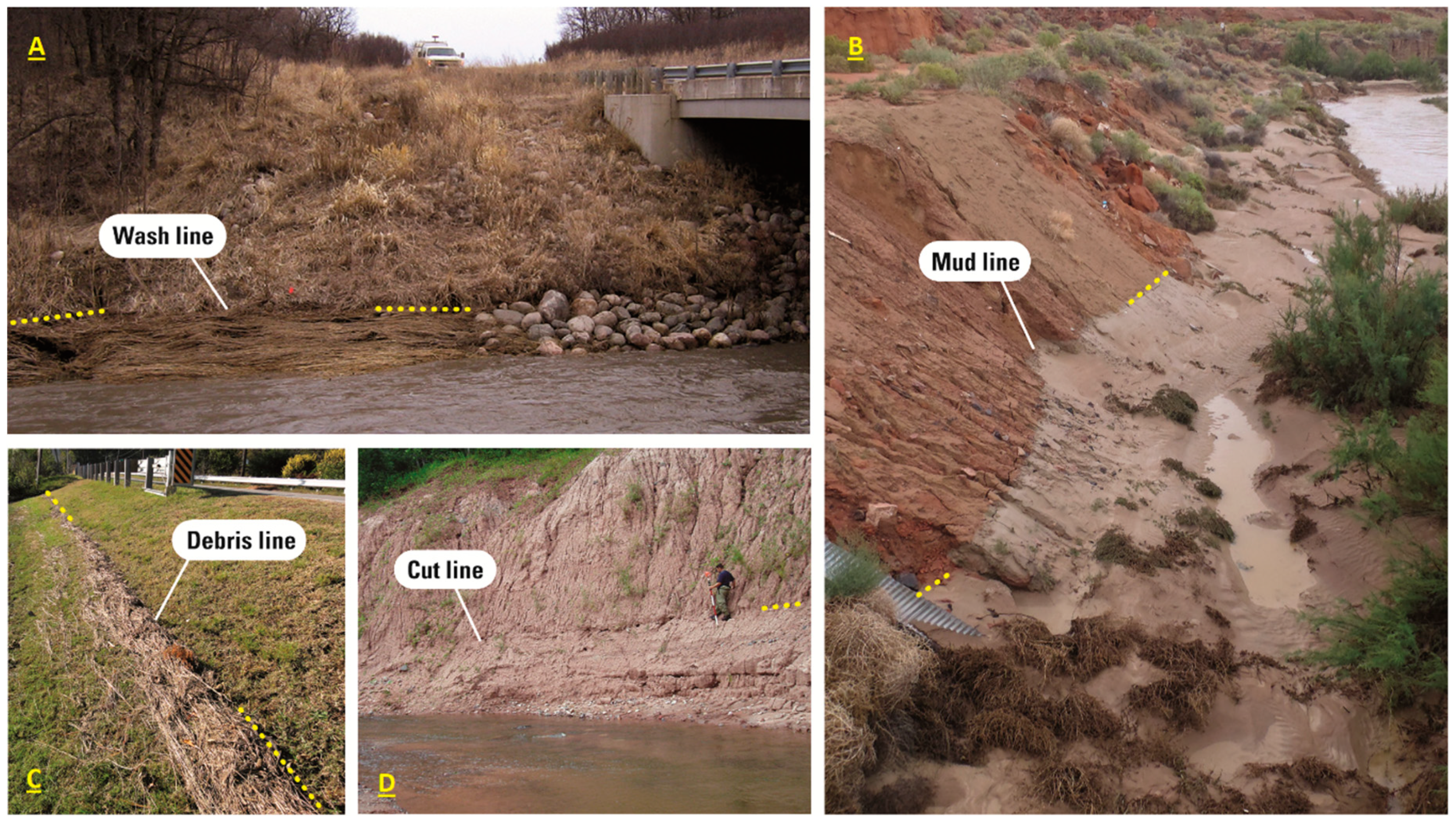
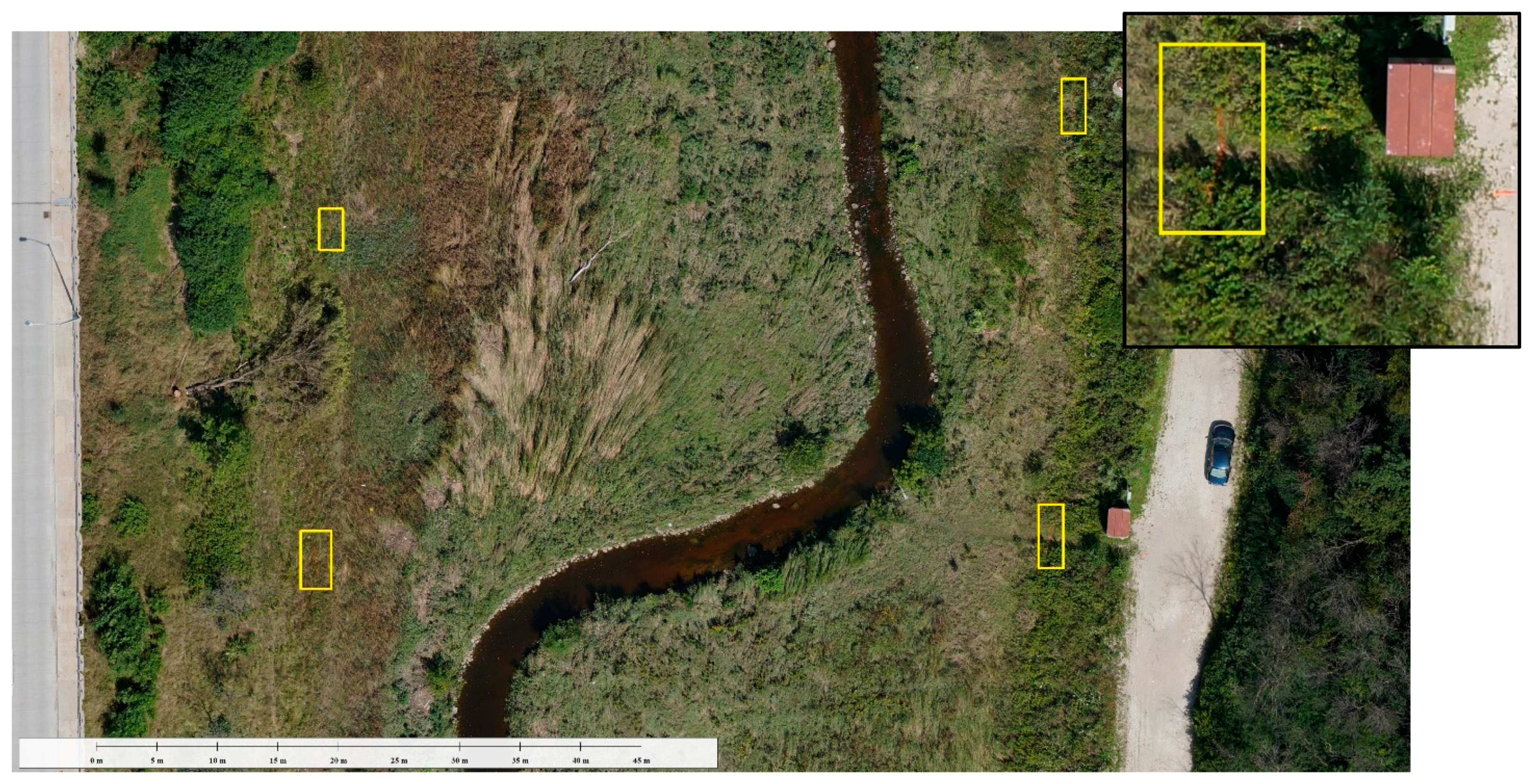
5]. HWMs are commonly the primary evidence of peak-flood stage and are left by many different types of floods in river channels, floodplains, and coastlines. Common types of HWMs left by floods are debris lines, wash lines, cut lines, and mud lines (Figure 1) [6]. Once HWMs have been measured, their elevations and locations are combined with terrain data, commonly cross-sectional surveys or digital terrain models (DTMs), and provide measures of the depth, extent, and cross-sectional area of floods.
Elevations and locations of HWMs can be identified and measured by various approaches, the most common being field reconnaissance and ground-based surveying. Typically, ground-based measurements are collected by survey-grade global positioning system (GPS) equipment soon after the floods recede. The inundation extent is often inferred by assuming that the HWMs represent the peak flood stage over the affected area [6]. This is done by overlaying the HWMs onto DTMs using geographic information system (GIS) software to produce maps of flood extent. However, point measurements of HWMs do not always provide sufficient resolution to accurately define a continuous inundation surface throughout the flooded area. Similarly, the horizontal and vertical resolutions of existing DTMs are generally too coarse, commonly greater than 1 m, and may not appropriately represent terrain features.
Alternatively, surveys using small unmanned aircraft systems (sUAS) conducted after floods have occurred can quickly collect data across relatively large affected areas (hundreds of square meters to multiple square kilometers) and provide orthophotographs (mosaicked images that have a spatial reference) with sufficient resolution to allow visual identification of HWMs [7]. Imagery data collected in a specific manner employing photogrammetric techniques using sUAS can be post-processed to generate accurate DTMs which can be used to map the location and elevation of the visually identified HWMs and the terrain features that were inundated. Post-flood HWMs and terrain data can be collected quickly and efficiently soon after a flood and before the HWMs naturally deteriorate. The sUAS provides the mobility to rapidly cover areas from more than one operating location in a short time, which can dramatically increase HWM data collection efficiency, the number of HWMs surveyed, and the safety of field personnel [8,9]. A further benefit of the sUAS surveys, relative to ground-based survey methods, is that high-spatial density data are generated to represent flood peak stages within sUAS data, which can then be used for flood mapping and calibration of hydraulic and inundation models.
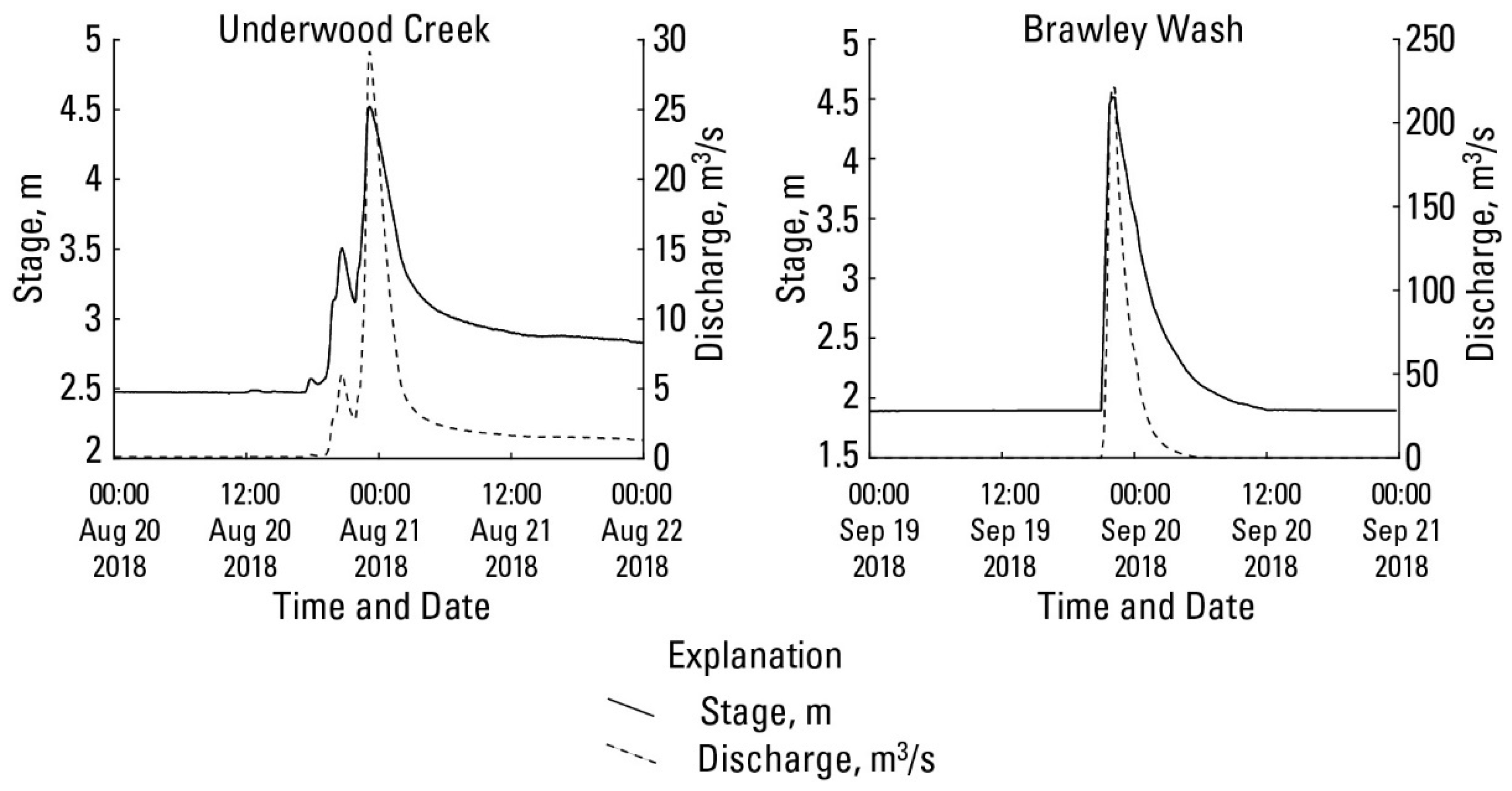
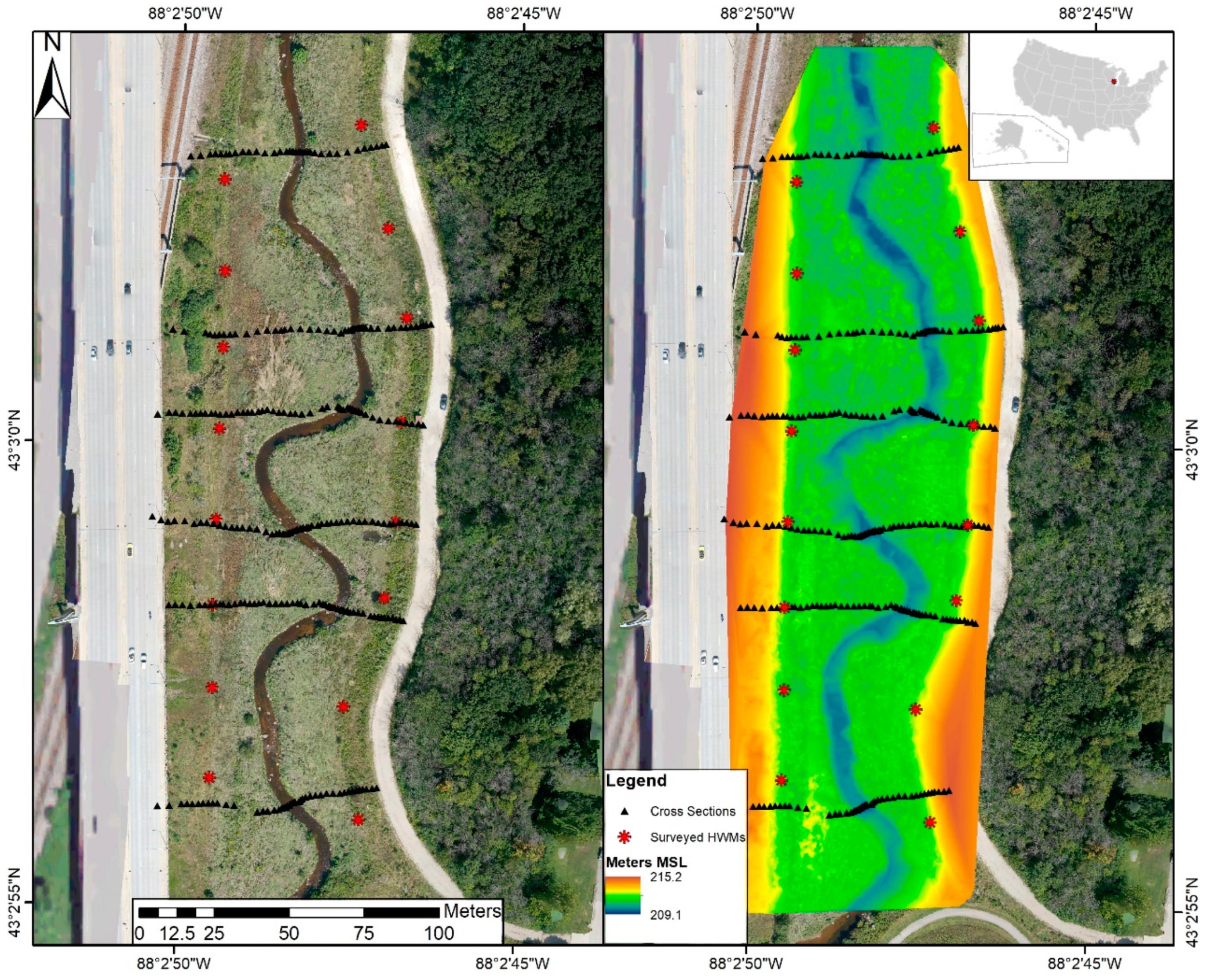
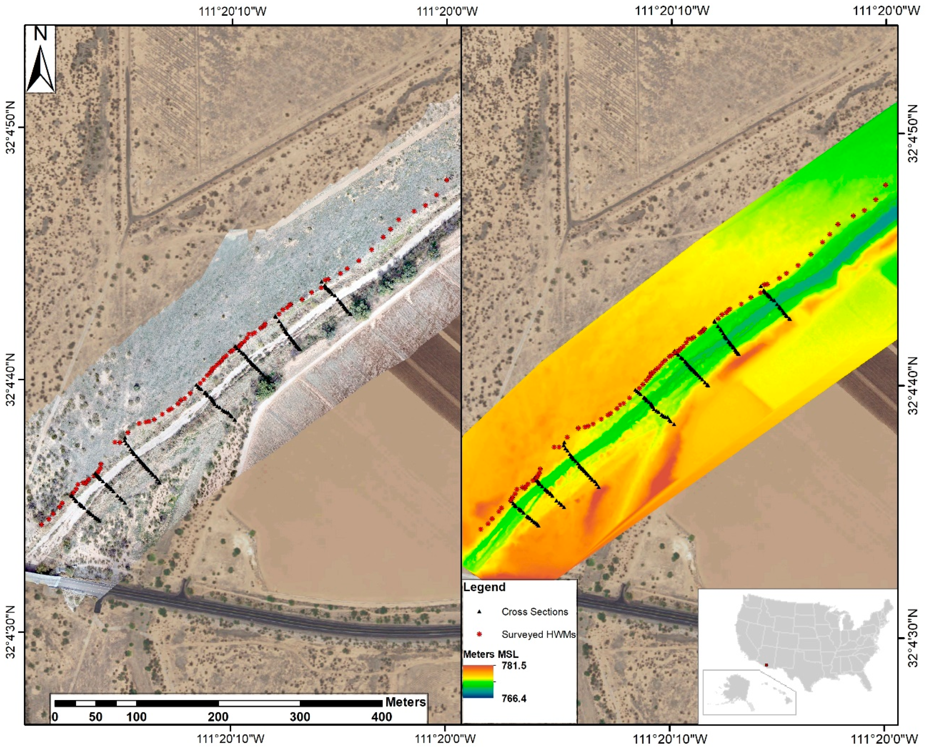
Here, we demonstrate and test the use of sUAS to characterize flood events on two small stream channels in the United States. The primary objectives are to demonstrate the sUAS survey techniques for locating and obtaining HWM elevations and inundated area to evaluate the accuracy of (1) DTM elevations derived from photogrammetric techniques and (2) HWM locations and elevations that were visually identified from orthophotographs and mapped using the DTM generated from the sUAS survey. The sUAS HWM elevations are evaluated by comparing them to ground-truth elevation data collected using GPS methods at the HWM locations and inundated terrain within the same stream channel. The orthophotographs generated from the sUAS are produced at fine enough resolution that individual HWMs can be identified at a specific pixel in the photograph, which then represents the location of the HWM. Elevations and coordinates of HWMs at those pixels are compared against GPS data to determine the accuracy and repeatability of this technique.
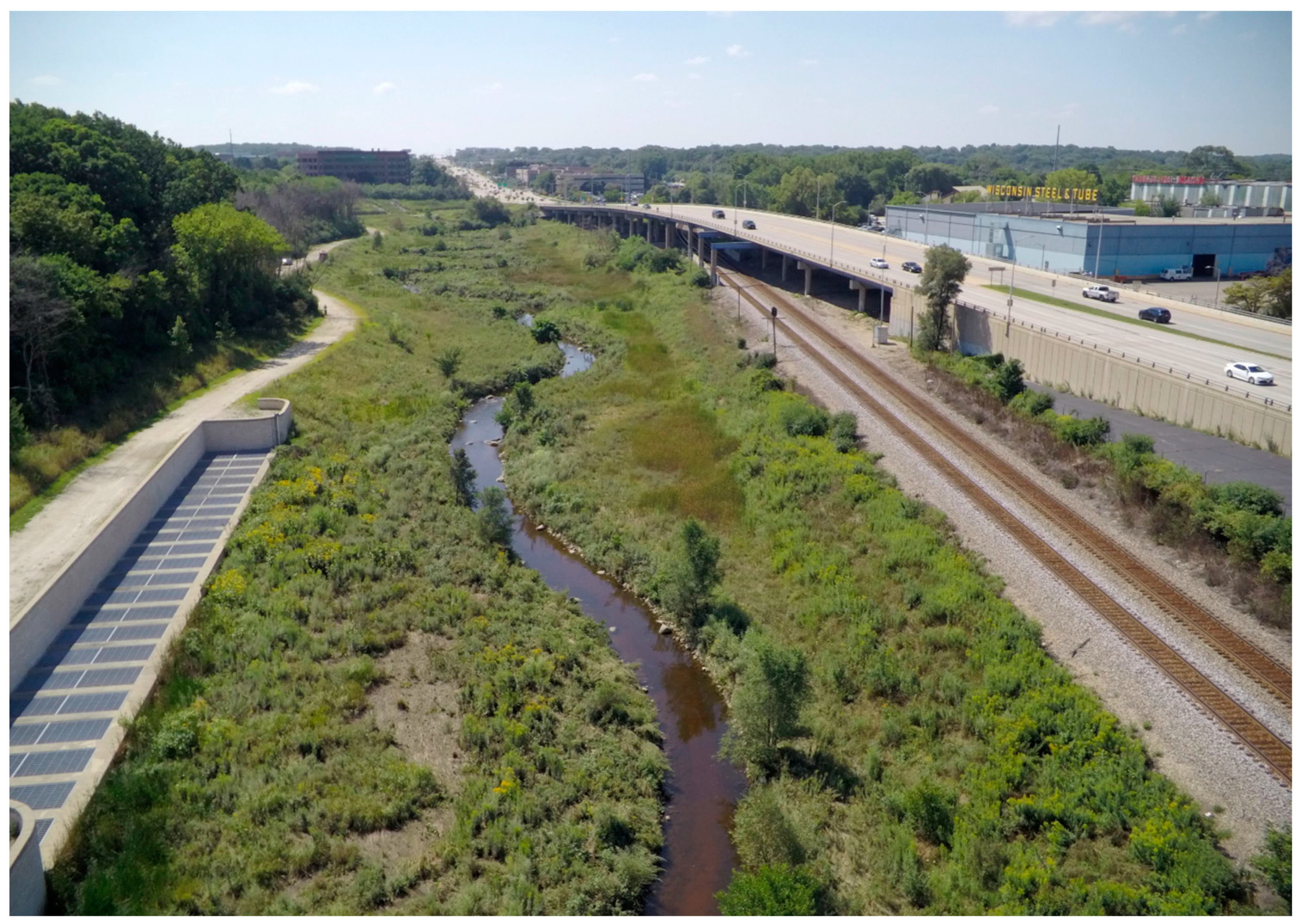
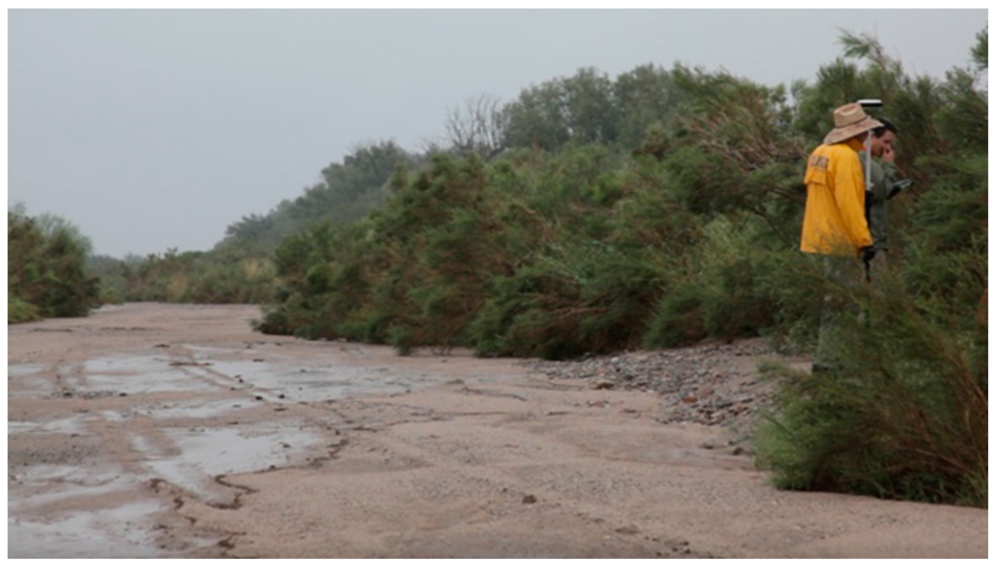
First, we describe the two field sites, Underwood Creek in Wisconsin, USA, and Brawley Wash in Arizona, USA. Then the GPS survey and sUAS survey methods, and the methods and results of the comparison of the HWM elevations from the GPS and sUAS methods are described. Finally, we describe field conditions that could limit the success of these techniques and discuss best practices and lessons learned for future post-flood sUAS HWM data collection. Our focus on examining the accuracy of using sUAS for post-flood data collection builds upon the work by Diakakis et al. [10]. Our assessment of increasing data collection efficiency in a post-flood environment complements the work of Smith et al. [11].

2. Materials and Methods

2.1. Site Descriptions

In this paper, we discuss the analysis of two small river reaches, Underwood Creek in Wisconsin, and Brawley Wash in Arizona, USA, to demonstrate and test the application of sUAS HWM survey techniques. Both sites experienced flooding in 2018 and have the requisite datasets: HWMs surveyed by GPS and high-resolution aerial photographs collected by sUAS using photogrammetric techniques in which HWMs were visible. Although these rivers and flood events are relatively small, the techniques demonstrated here can be scaled up and deployed to quantify the extent of HWMs typically found in much larger magnitude floods.
Our first study area was Underwood Creek, U.S. Geological Survey (USGS) gage 04087088, near the town of Wauwatosa in southeastern Wisconsin. This perennial stream drains a suburban area of 46.9 km2 and flows are influenced by local urban runoff from impervious surfaces [12]. The channel gradient is low (approximately 0.0025), and the main channel is incised and meanders through the floodplain. Tall grasses, cattails, and shrubs are prevalent in the channel and floodplain as seen in Figure 2. The flood being analyzed occurred on August 20 and 21, 2018 (Figure 3), inundating a heavily vegetated and terraced floodplain. Sixteen HWMs were surveyed using GPS surveying equipment on September 14, 2018 [13], explained in detail below, all of which were used for comparison with the sUAS survey. The sUAS survey was completed on August 23, 2018 [14], and cross-sections in support of hydraulic modeling were surveyed on July 17, 2019 [15] (Figure 4). Channel change is not suspected in the time between the surveys due to the well-established vegetation at the site persisting throughout the year. The peak discharge for the flood event on August 20, 2018, was 29.2 m3/s, derived from the stage-discharge rating [12].
Our second study area was Brawley Wash, USGS gage 09487000, near the town of Three Points, Arizona. The site has a drainage area of 2010 km2 [16] and is a sand-bedded ephemeral wash that flows only in response to heavy rain events that cause flash floods (Figure 5). The channel gradient is low, about 0.005, and the gage site often requires indirect measurements to quantify peak flows because of the flashy flows commonly observed in the region. Dense shrub and tree vegetation are present on the right lower and mid-overbank areas of this straight continuous channel, with intermittent shrub vegetation on the left lower overbank. The flow event studied was contained in the primary floodplain of the main channel and occurred on September 19, 2018 (Figure 3). The peak discharge of 220 m3/s [16] was calculated using traditional indirect discharge measurement techniques, which has a 5 to 10-year peak flood recurrence interval [17] (Figure 3). 78 HWMs were surveyed on the left bank of the stream in adittion to seven cross-sections using GPS equipment on October 1, 2018 [18], all of which were used for comparison with the sUAS survey (Figure 6). High-water marks were not found on the right bank during the field campaign. The reach was surveyed with sUAS on January 31, 2019 [19].

2.2. Ground-Based GPS Data Collection

The GPS surveys at both sites were conducted following USGS data collection standards [20]. The survey at Underwood Creek utilized a cellular-enabled Real-Time Network where the Leica GS14 GPS unit accessed multiple base stations in the region to find the absolute position of points during the survey. The GPS survey conducted at Brawley Wash was done using a static solution with the base station setup over a single point during the entire data collection. The data collected by the base station was sent to the Online Positioning User Service (OPUS) to tie in the position of the survey to NAD83 and NAVD88 datums [21]. The GPS-surveyed points have two different types of uncertainty associated with them, absolute position and model composition. Absolute position is associated with the accuracy of the base location, cell towers or GPS base station with OPUS correction, and generally are 0.02 m horizontal and 0.04 m vertical. This accuracy addresses how a model will plot on a map or in GIS and does not affect the relative positions between points. The accuracy of surveyed points in relation to each other, composition, is more important for generating a comparative model and establishing representative geometries and is what is important in this research. The uncertainty of composition for these models is generally 0.015 m both horizontally and vertically [20].
Uncertainty about the flood stage and extent is influenced by the equipment and survey techniques, as well as the conditions that form and represent the HWMs in the field. In addition to the minimal uncertainty caused by the GPS survey equipment, HWMs do not always represent a perfect measure of the water surface at its peak and HWMs rarely exhibit a smooth surface in situ. HWMs are formed by the interaction and deposition of material at the interface between the flowing water surface and the river’s bank, bridges or other structures, or stable vegetation, such as large trees. At this interface, the elevation of the HWMs can be affected by turbulence, surging flow, local influence from vegetation and channel-bed material, drawdown effects, pileup, among other factors which all commonly cause noise in the water-surface elevation. The HWMs can also degrade soon after the water recedes due to wind, rain, gravity, and cleanup efforts. Depending on where and when the HWM is measured, the survey data can show variability in the elevation of the measured surface in the reach. Under standard USGS HWM procedures, HWMs are assigned an uncertainty value to represent the vertical range of peak water surface that could be described by the HWM in the field [6]. The HWMs at both study locations are considered to be of excellent or good quality with a vertical uncertainty of 0.015 to 0.03 m [6].
Interpreting a continuous representation of the peak water surface elevation using the GPS HWM data is performed throughout the reaches at both study locations to properly compare data collected from the sUAS. This is done by using all the GPS point data collected in the field, coupled with survey uncertainty and HWM quality, to define a smoothed water surface elevation across the entire length of the reaches. In the two test cases here, the HWMs were of good to excellent quality, so all HWMs were weighted equally when establishing the spatial trend of the water surface. For each test site, a Locally Weighted Scatterplot Smoothing (LOWESS) curve [22] was fit to the GPS surveyed HWM data as a function of downstream distance to act as the measured water surface trend along each reach. Establishing a trend in the water surface that best fits HWM point data is common practice when conducting this type of data collection, where outliers are commonly ignored [5,6]. The water-surface trend is used in many different modeling approaches, many of which are sensitive to the overall slope of the water surface and are critical to categorize correctly [23]. HWM elevation data collected from the sUAS were compared to the LOWESS curves drawn at each study site.

2.3. sUAS Photogrammetric Data Collection and Processing

Overlapping color images of sharp focus and appropriate exposure were collected using the sUAS at both of the study locations. At Underwood Creek, data were collected with a DJI Inspire quadcopter and a Sony NEX5 camera. At Brawley Wash, data collection was done using a 3DR Solo micro-quadcopter and a fixed custom-mounted Ricoh GRII camera. Basic flight planning and command-and-control software were used to plan and execute area coverage, manage flight lines, and acquire photos with 60% photographic overlap, ensuring good stereo-photograph geometry for photogrammetric processing. Underwood Creek was flown at approximately 75 m above ground level under partially cloudy skies; the 0.163 km2 area was captured with 289 images. Brawley Wash was flown at approximately 90 m above ground level on a clear sunny day; the 0.278 km2 area was captured with 317 images.
Photographs at both sites that were collected by sUAS were processed in Agisoft Metashape [24] to develop a three-dimensional point cloud model, a DTM, and an orthorectified mosaicked image. Processing techniques and objectives may be referenced from the USGS National UAS Projects Office publication, Unmanned Aircraft Systems Data Post-Processing, Structure-From-Motion Photogrammetry [25]. Gradual selection techniques to statistically reduce model errors were used to establish tie-points that had a base-to-height ratio of 1:2.3 (reconstruction uncertainty = 10), a standard deviation of between 3-4 (projection accuracy 3-4), and a compositional pixel accuracy of better than 0.2 pixels (reprojection error 0.2–0.14). When the models are developed, ground control points are heavily weighted the ground targets that were surveyed by the GPS equipment with 0.02 m positional accuracy). Camera positions measured with GPS sensors onboard the sUAS were processed with looser tolerance (~10–30 m) as forward motion, capture and write times, and collection in ellipsoid height all negatively affect image position data compared to the GPS data. Once acceptable common imagery tie-points were established, data were processed to generate products including a three-dimensional point cloud model, a DTM, and an orthorectified mosaicked image.
The next step in the photogrammetric data processing procedure was the development of bare-earth DTMs. Raw, point-cloud data generated by prior steps include vegetation due to the capture of photographic pixels on vegetated surfaces visible from the sUAS’s bird’s-eye view. By contrast, GPS surveys of HWMs measure the position of the HWM on the bank’s bare-earth surface, beneath any vegetation. In order to obtain comparable data sets, near bare-earth DTMs needed to be processed and produced for both study sites. Classification tools within Agisoft Metashape [24] and Global Mapper [26] were used to build the bare-earth DTMs. Classification steps included removing outlier data, noise filtering, color identification, and geometric classification tools to remove or classify points that represent features that are not ground. Challenges in vegetation classification include plant material that has a similar color to ground surfaces (dormant grasses), vegetation that obscures all view of the ground surface when viewed from above, and oversimplification of vertical surfaces below dense vegetation in the channels in areas where banks are steep and undercut. Ultimately, a combination of automated and hand-editing techniques was used to produce the bare-earth DTMs used in the subsequent analyses.

2.4. Evaluating sUAS Surveys for Collection of Post-Flood Data

The data collected by sUAS were first examined to determine if HWMs were clearly visible in the orthophotographs, as some HWMs can be faint, small, and difficult to distinguish. To accurately map HWM elevations, HWMs must be clearly identifiable within the orthophotograph, making crisp and clear imagery imperative. The orthophotographs were examined to determine if HWMs were visible in both stream reaches when zooming in to the photographs using GIS software.

2.4.1. Comparing GPS Surveyed HWM Elevations to DTM Elevations

The accuracy of the sUAS surveys for obtaining flood peak-stage and channel elevation was evaluated first by comparing sUAS elevations with those measured by GPS surveys. The elevations from the GPS surveys were treated as the control or “true” values for the comparisons. The first comparison evaluated the DTM elevations generated by the sUAS survey and photogrammetric data at the exact locations where the GPS points were collected. Using Global Mapper GIS software [26], the orthophotograph was draped over the DTM, and the GPS points were rendered onto the orthophotograph and DTM. The positions of the GPS surveyed HWMs and channel topography were duplicated in the GIS software by creating point features. The point locations were then assigned the underlying sUAS generated DTM elevation values and corresponding elevations were compared.

2.4.2. Comparing GPS Surveyed Cross Sections to DTM Elevations at Surveyed Points

The next comparison evaluated the elevations of cross-sections surveyed in each channel. This comparison took the same approach when evaluating the HWMs compared to the DTM elevations described in the previous section but was done using the surveyed cross-section points. This analysis is particularly important because an accurate cross-sectional area is important in hydraulic analysis, such as multiplying the area by the mean velocity in meters per second to obtain a discharge in cubic meters per second. Additionally, when cross-sections are surveyed in situ, field staff make informed decisions about what points to survey at critical inflections in the channel that best characterize the overall shape of the channel, ignoring vegetation and objects that are perceived to be mobile, like floating vegetation debris or trash litter accumulated by flood inflow. When comparing cross-sections in the GIS environment, points were picked directly under the surveyed points just like the prior HWM analysis, benefitting from the field staff’s decision making. GIS also allows an analyst to pull points under a line by a set number or regular interval, or inflection points, but these methods may over-generalize the channel, dramatically changing the true cross-sectional area. These techniques do not account for the influence of objects that should not be included such as vegetation artifacts or debris mats or litter.

2.4.3. “Blind” Hydrologist Selected HWMs from sUAS-based GIS Products

The next comparison assessed error associated with visual identification of HWMs using the orthophotograph and the measurement of HWM elevations obtained from the DTMs, all of which were done using the remotely-sensed data products through GIS. For this comparison, GPS survey elevations were not available at every location along the reach to serve as “true” elevation comparisons. Instead, the HWM elevations were compared to an estimated flood-peak surface profile using a LOWESS fit [22] of the GPS elevations in the downstream direction. In this evaluation, three separate hydrologists identified HWMs from the sUAS data along the river reach to test repeatability and the variability of different interpretations of HWM locations from orthophotographs. The three trials were done without access to the control data set, so all HWMs and elevations were identified directly from the sUAS data. The selected HWMs were plotted in a downstream distance along the river’s thalweg, and the results of the three trials were compared to the LOWESS curves generated from GPS survey point data that describe average water surface slopes at each study location.

2.4.4. LOWESS Curve Fit to Hydrologist Selected HWMs compared to GPS LOWESS Curve Fit

The final comparison assessed the difference between a LOWESS curve of the visually selected HWM elevations and the LOWESS curve of the GPS-measured, or true, HWM elevations. Hydraulic modeling often requires a best-fit line to represent the slope of the water’s surface during a flood event commonly profiled through the collection of HWM point data. HWM data are typically noisy and contain outliers, as the water surface is rarely a smooth linear plane at the peak of floods, requiring a smoothed curve to be developed to represent the overall trend in the water’s surface. Traditional GPS field surveys often generate points that are used to profile the continuous water surface, averaging a line between points with weighting dependent upon point quality, with inflections at the different cross-section locations. This study used a LOWESS curve that fits a curve to the HWMs, creating a continuous water surface that may better represent the dynamic conditions in the reaches. A locally weighted and smoothed line or curve better represents data used in hydraulic modeling when compared to the likely noisy point data collected by surveyed HWMs. LOWESS curves were compared for the two data sets, the “true” GPS field survey data compared to the “blind” sUAS-based GIS selected data by the three hydrologists which represent the final comparison.
For each comparison discussed above, the mean error (ME) and mean absolute error (MAE) of the residual differences of the two separate measures were calculated. The ME statistic was used to assess the potential vertical bias in the sUAS survey that may result from the effects of vegetation. Vegetation in the photogrammetric data collected using sUAS could result in higher measurements of elevation in the DTM, relative to bare-earth elevations. The MAE statistic was used to compare the variability between the measured and true values to gauge the differences between the control and sUAS data. The assumption was that the lower the MAE or magnitude of error, the higher the confidence in the water surface profile established along the river’s banks.

3. Results

3.1. HWM Identification in the sUAS Orthophotographs

At Underwood Creek, HWMs were identified along the margin of the flood on both banks by the color change caused by vegetation that had been laid down during the event and in some locations, by debris lines. To aid identification at Underwood Creek, high-visibility paint was applied by the GPS survey team at multiple locations to identify HWM locations along the river’s banks (Figure 7). This technique proved valuable to aid HWM identification in the orthophotograph collected using sUAS. At Brawley Wash, HWMs were identified as flattened vegetation coupled with almost continuous debris and wash line along the left bank (Figure 8). The HWMs were easily identifiable in the sUAS generated orthophotographs at both study sites.

3.2. Terrain Modeling Results

Point cloud data were classified into ground and vegetation classes, hand edited to best represent a near bare-earth model, and then used to render a triangulated irregular network (TIN) surface for each study site. The TIN model creates a continuous surface and interpolates to fill in areas of sparse data because vegetation has been removed. A DTM was constructed from the TIN models with a 3-cm pixel resolution to create an elevation background data set at the averaged positional accuracy of the survey-grade GPS data collected at ground targets. While the compositional accuracies of the GPS data and the sUAS derived models were around 1.5 cm or better, the positional (absolute) accuracies of base points and each respective survey point was 2 cm horizontal and 4 cm vertical. High compositional accuracy is important for individual models as the goal is the best representation of the natural environment, especially when those models are driving further analysis such as hydraulic modeling. Though the models are generally more accurate in composition than the positional accuracy of the GPS, using the GPS accuracy for resolution ensures appropriate confidence is given to any individual part of the model.
Holes in the terrain data caused by the removal of vegetation were interpolated and filled by converting sUAS collected points to a TIN and then to a DTM. This is a common occurrence when doing vegetation removal using photogrammetric data because the model only contains data from what is visible from above. The Underwood Creek DTM had a noisy overbank surface on the floodplain due to the dense, partly laid-over vegetation present on the banks. These conditions effectively created a DTM that was slightly higher than the actual ground surface by approximately 0.4 m. The DTM for Brawley Wash characterized the upper overbank conditions well, based on comparison with GPS survey data in that area where vegetation was mostly grasses, but the steep primary channel banks and mid-height vegetation at the overbank transitions proved problematic, causing both oversimplifications of the bank transitions and residual vegetative noise. The model containing vegetation compared to the resultant near bare-earth DTM from Underwood Creek and Brawley Wash can be seen in Figure 9 below.

3.3. Evaluating the DTM and sUAS Elevations

The first comparison between GPS surveyed points and data derived from sUAS compares the GPS surveyed HWMs to the elevations of the DTM at the same location on the river’s banks as described in Section 2.4.1. In theory, the elevation of the GPS collected points and the elevation of the DTM at that location should be very close, within the compositional error of the surface model and GPS equipment, about 0.01 to 0.04 m since they are collocated in the same position. The horizontal position of the GPS points was plotted on top of the DTM elevation sampled at that same location, and elevations from the GPS survey and the sampled DTM location are compared. The ME and the MAE were calculated to compare the control data to the sUAS data. The relative ME and the relative MAE were calculated to compare the overall trend in the water surface in the reach, a critical parameter when conducting the hydraulic analysis. The results of this comparison can be seen in Figure 10. Some variability between the control and sUAS datasets that can be seen in Table 1.
This comparison shows the difference in performance between a fully vegetated site, (Underwood Creek) and a site with little vegetation (Brawley Wash) when using sUAS mapping techniques. Underwood Creek showed an overall ME of 0.26 m, whereas Brawley Wash showed a ME of only 0.02 m. This positive bias between the true and sUAS measured elevations is assumed to be attributed to the vegetation located in the reach that caused the DTM to be erroneously high in elevation. In contrast, Brawley Wash, with little to no vegetation on the banks near the HWMs, showed an overall ME much closer to the true elevation measured by the GPS. This trend can also be seen in the relative ME of the overall trend in the water surface being 46.7% at Underwood Creek and just 1.0% at Brawley Wash.
A LOWESS curve was fit to describe both the GPS and sUAS elevations at each surveyed HWM, and the results of their comparisons are similar to the point data comparison discussed above. Underwood Creek sUAS data ME was 0.28 m higher than the GPS survey, which is assumed to be due to the effects of vegetation, but had a similar downstream trend of water-surface slope as the GPS data, and Brawley Wash sUAS data ME was just 0.01 m (Table 1). Using point data to interpret the water surface profile along the river reaches is important for hydraulic modeling and inundation mapping. The downstream slope is an important component in these applications and can have a large effect on the modeling result, especially in low-gradient river systems.
The second comparison between GPS surveyed points and data derived from sUAS compared GPS surveyed cross-section elevations with elevations of the DTM at the same locations as described in Section 2.4.2. This was done in the same manner as the HWM comparison described above, where the position of the GPS surveyed point was used to compare the ground measurement against the DTM elevation at the same location. The results of this analysis can be seen in Figure 11. Some sections compare well, for example, sections 1–3 at Brawley Wash are all less than 0.2 m ME (Table 2). Sections 1 and 3 are less than 0.29 m ME at Underwood Creek (Table 2) even though the banks are covered with dense vegetation which in many places obscures the ground.
Other sections have fair results when streambed elevations collected from GPS and sUAS are compared. Sections 4 and 7 at Brawley Wash compare within 0.41 m ME and sections 5 and 6 at Underwood Creek were within 0.46 m ME. This is again believed to be an artifact of the dense vegetation present on the channel banks, which limits the ability of the sUAS to photograph the ground surface. As mentioned above, water can cause issues for photogrammetric data processing techniques, and in this case, the actual bottom elevation of the channel was not measured at some locations in the sUAS terrain data, although the difference is quite small, about 0.20 m ME.

3.4. Evaluating the sUAS Surveys for Identification and Mapping of HWMs

The third and final comparison assesses differences in the HWM water surface trend based on blindly selected HWMs with the GPS measured HWMs as described in Section 2.4.3 and Section 2.4.4. The HWMs were chosen using the orthophotograph and mapped using the DTM by three different hydrologists at both sites. Because this is a subjective process that may include operator error, the exact same analysis was performed independently by each of the three hydrologists. Hydrologists were instructed to use only the orthophotograph and hydraulic judgment to select HWMs that they felt best represented the HWM profile in the reach. Hydrologist #1 chose 18 HWMs at Underwood Creek and 25 HWMs at Brawley Wash, Hydrologist #2 chose 19 and 20, respectively, and Hydrologist #3 chose 28 and 42, respectively. The results of these trials compared with the 16 and 78 HWMs surveyed using GPS are shown in Figure 12.
The first evaluation of these trials assesses differences between the LOWESS fits of the GPS and the sUAS-derived HWM point data as described in Section 2.4.3 and Section 2.4.4. At Underwood Creek, the three hydrologist-chosen HWM elevations had ME = 0.05 m or less and MAE = 0.20 m or less (Table 3) compared to the LOWESS fit of the control data. The relative ME compares the overall trend in the water surface in the reach to the control data; results for Hydrologist #1 and #3 show low bias with relative ME of 2.2% and 0.3% respectively. Results for Hydrologist #2 show a larger bias of -8.1% in the water surface trend comparison. The relative MAE shows a range of 22.6% to 35.7%.
The next evaluation at Underwood Creek compares the LOWESS fits of both the GPS and sUAS measured HWM data as described in Section 2.4.4. The ME of the three hydrologist-chosen data set compared to the control data were -0.04 m to 0.01 m. The MAE comparing the data sets was 0.03 to 0.09 m. Promising results were also found when comparing the relative error between the hydrologist-chosen HWMs and the control data. Trials had relative ME of −7.9 to 1.1% and had relative MAE of 4.5 to 16.1% Table 3.
At Brawley Wash, the three hydrologist-chosen HWM elevations had less than ME = -0.06 m and MAE = 0.09 m error compared to the LOWESS fit of the control data as described in Section 2.4.3 (Table 4). This shows that the sUAS-measured data compared well to the control and that the data had minimal scatter because the MAE was low. The relative ME compares the overall trend in the water surface in the reach to the control data, results show an ME of −2.4 to −0.6% and had MAE of 2.3 to 3.6% (Table 4).
The next evaluation at Brawley Wash compared the LOWESS fits of both the GPS and sUAS-measured HWM data as described in Section 2.4.4. The ME of the three hydrologist-chosen data set compared to the control data were −0.07 to −0.03 m. The MAE comparing the data sets was within 0.04 to 0.07 m. Promising results were also found when comparing the relative error between the hydrologist chosen HWMs and the control data. Trials had relative ME of −3.1 to −1.2% and relative MAE of 1.6 to 3.1% (Table 4). This result shows that the data measured using only sUAS fits the control data well with minimal scatter and provided an accurate measure of the peak water surface slope in the reach.

4. Discussion

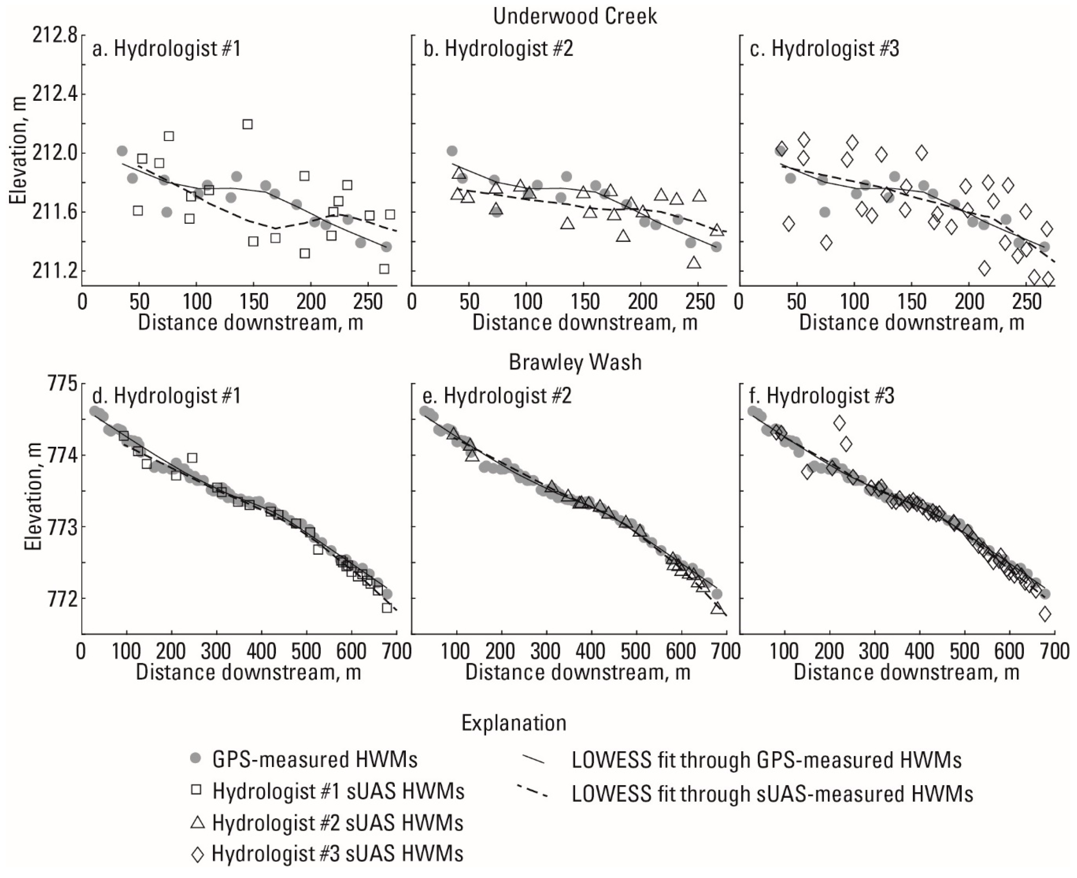
The results presented here show that locating and measuring HWMs using sUAS and photogrammetric techniques is possible, and for the cases examined, proved accurate compared to data obtained using traditional GPS survey methods. The noteworthy finding in this research was the results of three comparisons at both study sites demonstrated the ability of flood hydrologists to successfully locate and measure HWMs accurately using only the products collected by the sUAS. The results from the three trials performed independently by three hydrologists also showed that skilled identification and interpretation of HWMs within the sUAS data resulted in the best comparison to the control data.
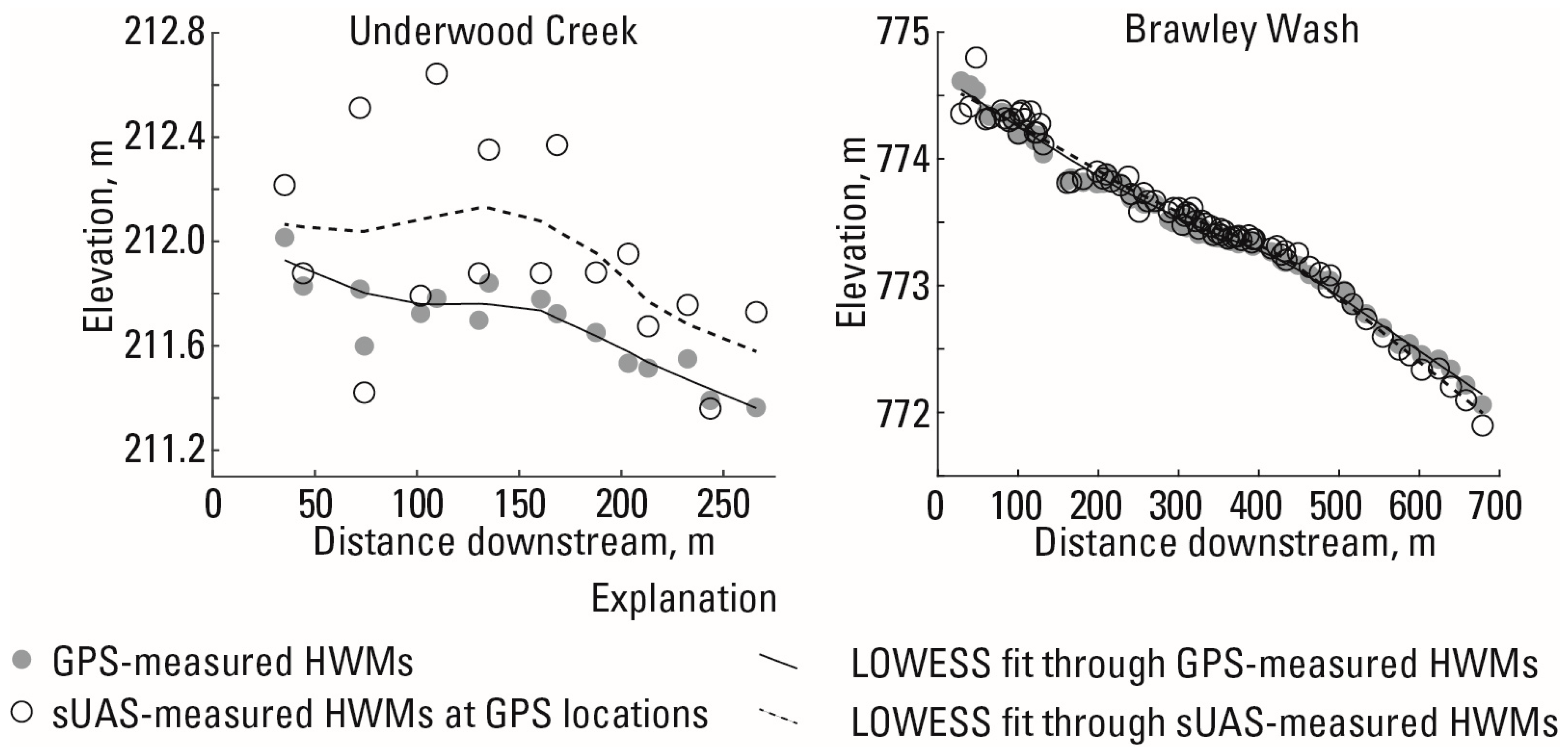
The most important findings were that the hydrologist-selected marks provided the best results in this analysis. The information presented in Figure 10 and Table 1 shows the results of the HWM location surveyed with the GPS and compares it to the elevation of the DTM at that same location. The results of this analysis at Underwood Creek were fair, ME = 0.26 m and MAE = 0.33 m (Table 1), but that amount of uncertainty would not be considered highly accurate for hydraulic modeling applications. However, the results of the hydrologist-selected HWMs at Underwood Creek showed better results, ME = −0.05 and MAE = 0.20 (Table 3). This shows that the style in which HWMs are surveyed using ground-based methods compared to sUAS identification might be different. When field teams collect HWMs, they have the opportunity to survey HWMs using the GPS in locations that may not be visible from above, which was the case at Underwood Creek. The HWMs selected by the three hydrologists were only HWMs that were visible from above and were likely HWMs that were located in areas free of vegetation and on the ground, not located underneath vegetation. This produced a better result in all cases and shows that even sites with heavy vegetation can be analyzed to produce accurate measurements of HWM using sUAS techniques.
Because the study plots at Underwood Creek and Brawley Wash had such different conditions, particularly the type of HWMs left by the flood and the amount of vegetation present in the channel, this study has shown conditions where techniques using sUAS would be promising, and conditions where photogrammetric data collection might not yield adequate results. As discussed, vegetation is a limitation for this type of data collection because it obstructs the view of the ground surface from the camera. An inconsistent bare-earth model results in areas within the DTM being artificially elevated. Targeting areas away from vegetation where the HWMs reside at or near the ground surface will produce the most defensible results when using these techniques, as was shown in comparison three where the hydrologists selected marks that were visible from above and likely on the ground.
Our results provide guidance for planning sUAS photograph collection campaigns to document flooding extent. Important factors to consider when planning sUAS flights include coverage area, flight altitude, resolution of the camera, and desired accuracy of the resulting HWM survey. Data collection and ideal pixel resolution can be guided by the resolution necessary to positively identify HWMs. Whether the flood evidence is a debris line, sediment color change, laid-down vegetation, or a cut-line in a bank, 4–6 pixels are needed to discretely identify that object or change in surface representing the HWM. For this study, the derived orthophotograph for each project area provided a single measurable photographic product at 2.33 cm2 pixel size or smaller which provided the resolution required to positively identify the HWMs at both study locations, despite their geographic and geomorphic differences. If the HWMs investigated are less apparent than discussed in this research, then higher resolution orthophotographs would be needed and could be achieved with better camera sensors or by flying closer to the surface (lower altitude). In the case of fine seed lines, positive results might not be possible from sUAS collection if the HWM cannot be clearly identified in the orthophotograph.
Sound close-range photogrammetry techniques and a strong understanding of digital camera setup are critical for collecting accurate DTMs using sUAS. The near-nadir view used for data collection provides the most accurate compositional data but is limited in profiling complex vertical features. In areas of obscuring or overhanging vegetation, data collection at 10–15 degrees oblique in addition to nadir may help fill in ground surfaces and help with point classification, reducing data gap sizes. Shutter speeds too slow for the flight height or speed will create motion blur. Inappropriate aperture settings can over or under-expose imagery and potentially sacrifice depth of field. ISO settings too high (over 800) reduce crispness and clarity in the pixels and may create difficulties identifying features. These and other camera-specific settings need to be considered together to create clear and crisp photographs to feed photogrammetry analysis and produce accurate DTMs.
Point cloud processing algorithms are constantly advancing in modeling and GIS software, including the software packages used for this study, Metashape [24] and Global Mapper [26]. As photogrammetric data sets become increasingly common, the software packages are improving, furthering the ability to classify and edit photogrammetric data. Additional research is needed to establish more robust techniques for creating bare-earth models from photogrammetric data sets. Ultimately, the more accurate the bare-earth model, the more accurate measurements of HWMs in vegetated areas will be when using the sUAS techniques presented here.
Though out of reach for most potential users due to cost, commercial sUAS size aerial light detection and ranging (lidar) sensors are increasing in availability while decreasing in price. Lidar is the industry standard for generating point cloud models that can penetrate vegetation. This allows for not only a bare-earth model by only using the lowest or last returns, but also models of vegetation that can be analyzed, potentially providing useful information when looking for changes in channel roughness. Additionally, scanning sensors that mount to sUAS do not rely on rotating mirrors, motorized parts, and are generally lighter weight are becoming available and will lead to more accurate terrain data. Though these sensors currently are lacking in data density and point accuracy, this advancement represents progress in the field. The increasing availability of lidar means the subjective and possibly inaccurate process of classifying photogrammetric point clouds in order to make a bare-earth DTM could become unnecessary. Available aerial lidar models will also create comparative data sets to further determine utilities and deficiencies of photogrammetric data and is an opportunity for further research.
Identifying and measuring HWMs using sUAS has implications for data collection efficiency and personnel safety. To document widespread flooding, such as storm surge or inundation due to extreme precipitation, runoff, and surge events, survey teams must travel to many different locations to document HWMs with traditional methods. If operated from an area with a clear and safe viewshed, sUAS can access large areas and are not inhibited by localized ground conditions or hazards. This allows for imagery and topographic data collection over a much larger area and with more complete spatial coverage compared to traditional data collection methods. Additionally, sUAS can collect data in areas that are inaccessible after natural disasters due to inundated roads, closed bridges, or other obstacles, while the range of sUAS surveys reduces the number of locations and time spent traveling. sUAS data collection after floods can be completed in less time, with less physical exertion by personnel, and with less exposure to hazards.
Traditional surveys often require extensive hiking over rugged terrain with dense vegetation and difficult stream crossings to locate HWMs and survey cross-sections. Complete topographic data throughout a reach can be collected efficiently using sUAS, whereas traditional surveys provide limited cross-section data that are time-consuming and often challenging to collect. When collecting flood data with field crews and GPS survey equipment, the data collected are limited to the conditions seen on the ground at the time of the survey. Additionally, cross-sectional data is collected in parallel strips at a distance sufficient to characterize slope and fall between locations. This type of data collection benefits from significant field experience and might be limited by access, time, topography, and equipment requirements. sUAS collection can survey a complete inundation area rapidly without the need for complete physical access. Additionally, the models generated might be used for countless analyses with a wide variety of hydraulic software packages to best fit the complex conditions seen during flood events. Cross-sections may be rendered from DTMs at any interval or distance and are not limited to access. Further, complete DTMs may be used in two-dimensional hydraulic models to represent the complex terrain inundated, not limited by the uncertainty and assumptions between individual cross-sections. A more complete understanding of the natural environment and the complex interactions occurring during floods may be gained from more complete and holistic models.

5. Conclusions

We demonstrate that post-flood HWMs can be reasonably (within acceptable error) identified and mapped using sUAS-collected imagery processed using photogrammetric techniques. These techniques can increase data collection efficiency after natural disasters and major flooding while also keeping field personnel in potentially safer positions. The first important finding is that when the photogrammetric data sets are collected with appropriate ground control, the DTMs allow HWMs to be identified with low positional bias compared to the GPS-surveyed HWMs. Secondly, for the two cases presented, HWMs are clearly visible in orthophotographs with a typical resolution for sUAS-derived products. HWMs that were clearly visible include wash lines, debris lines, and mud lines, as well as HWMs depicted by vegetation that has been laid over by the flood.
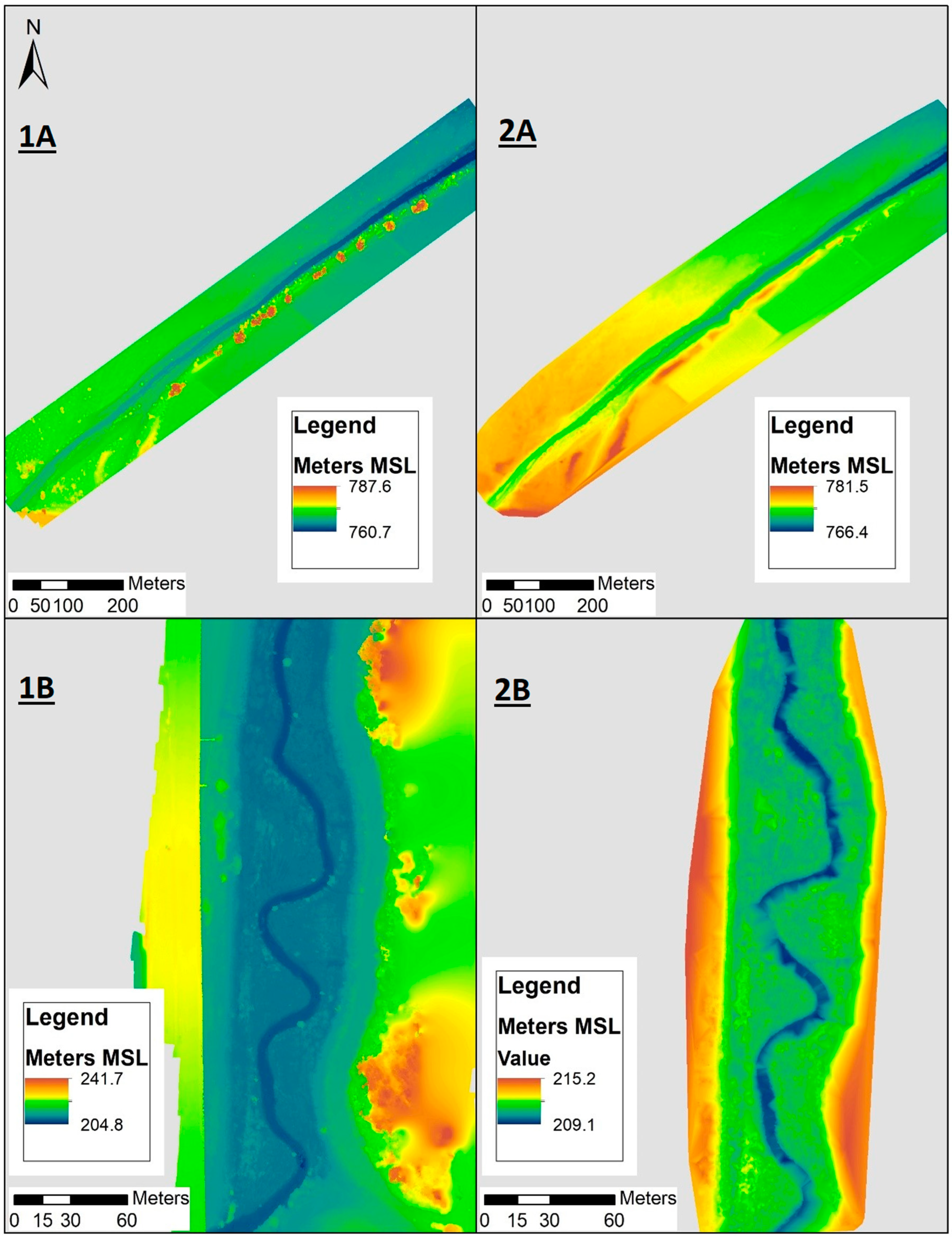
Vegetation is an important factor to consider when deciding whether to apply these sUAS-based HWM survey techniques. To accurately identify HWMs and map terrain elevation, images collected by the sUAS must contain pixels that represent the ground surface. In areas where tree canopy and thick vegetation dominate, aerial images may only capture pixels of the vegetation and therefore the terrain products that are produced do not accurately represent the elevation of the land surface in those areas. This can be seen in the results when comparing the two study sites investigated here with points collected with GPS surveying equipment. The results show Brawley Wash was mainly free of vegetation at the HWMs and closely reproduced the GPS surveyed data, within 0.02 m ME, compared to Underwood Creek where vegetation affected the accuracy of the bare-earth model at the HWMs and produced a 0.26 m ME.
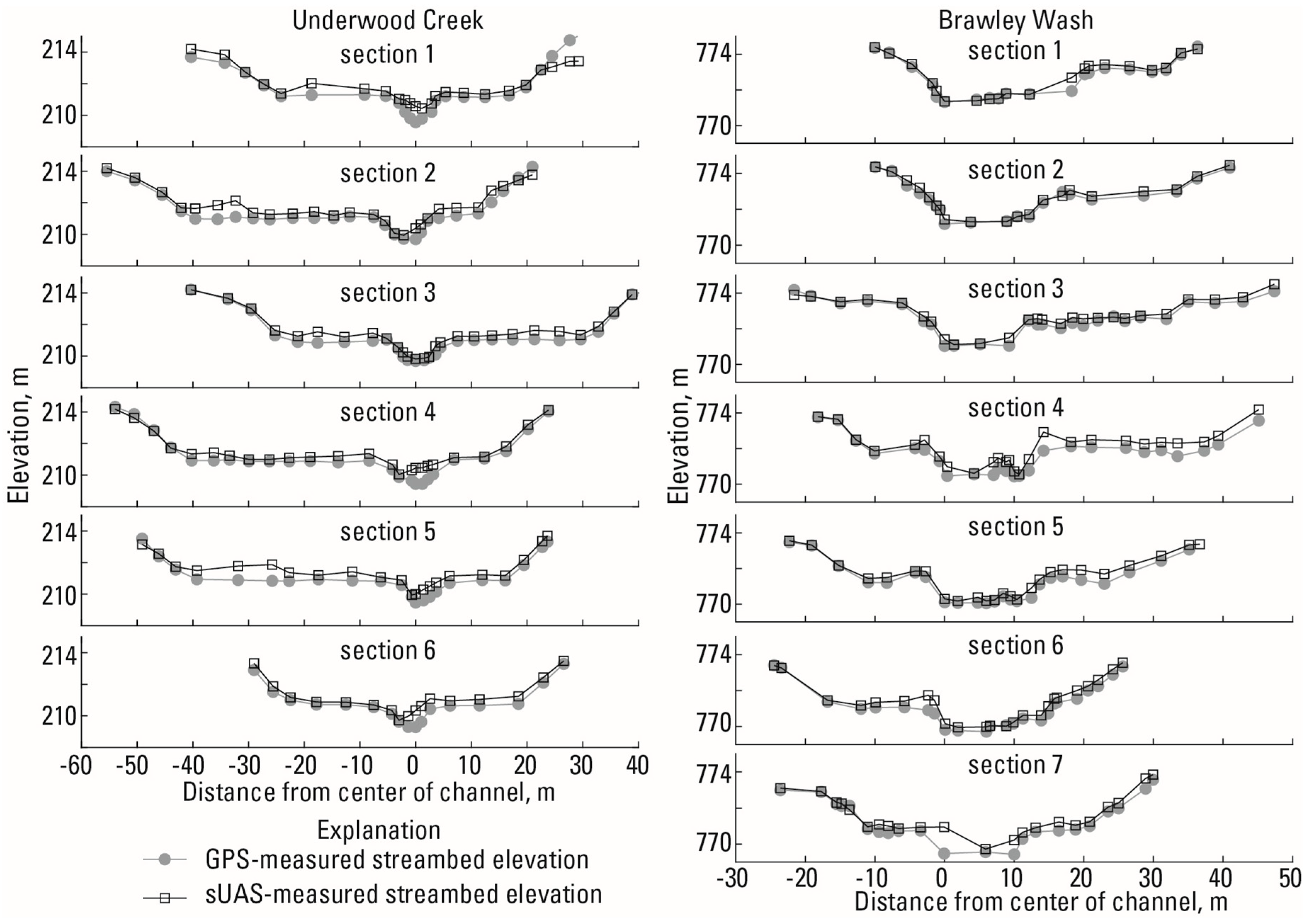
Vegetation has similar effects on the bare-earth model when comparing measurements of the cross-sections in both of the study locations. Both of the reaches contained dense stands of vegetation in places that limited the ability of the sUAS to photograph the ground surface at these locations. This caused varying success when comparing GPS measured cross-sections to sUAS-measured sections. Cross-sections 1 and 3 at Underwood Creek and 1–3 at Brawley Wash compare well to the GPS-collected data. However, cross-sections 5 and 6 at Underwood Creek and 7 at Brawley Wash show deviation from the actual ground-surface measurements. Cross-section data collection for hydraulic modeling requires specific locations of sections based upon channel slope and width. If sections cannot be located in areas free of vegetation where the DTM is proven accurate, field measurements might still be required to achieve accurate measures of the land surface.
sUAS-based surveying is proving to be a promising tool in post-flood data collection. Advancements in flight time and lift capabilities, coupled with the miniaturization of sensors such as high-resolution cameras and aerial lidar sensors, could increase sUAS collection in this field. Further analysis is needed to compare lidar data to photogrammetrically derived models, but ultimately a combination of lidar and stereo photography might provide the best representation of the natural environment with and without vegetation for complete hydraulic models. Still, depending on the absolute accuracy needed and the implications of the resultant data (i.e., flood inundation mapping for legal designation) ground-truthed data might be most appropriate. With an understanding of the available tools, their benefits and limitations, managers are empowered to tailor a response effort to the known field conditions, the legal implications of the data collected, and need for field personnel efficiency and safety.

Author Contributions

Project conceptualization: B.T.F., G.P.D. Methodology: B.T.F., G.P.D. Validation: B.T.F., G.P.D., C.E.B.; Analysis: B.T.F., G.P.D., J.E.D., C.E.B. Investigation: B.T.F., G.P.D., J.E.D., C.E.B. Data curation: B.T.F., G.P.D., F.A.F. Writing—original draft: B.T.F., G.P.D., J.E.D., C.E.B.; Writing—review and editing: B.T.F., G.P.D., J.E.D., C.E.B., F.A.F.; Visualization: B.T.F., G.P.D., J.E.D., C.E.B.; Funding acquisition: B.T.F., G.P.D. All authors have read and agreed to the published version of the manuscript.

Funding

The data collection an Underwood Creek was funded with support from the Great Lakes Restoration Initiative with support from the U.S. Army Corp of Engineers. The data collection at Brawley Wash was funded by the Arizona Department of Transportation and Pima County Flood Control. Analysis and publication costs were funded with support from the U.S. Geological Survey Hydrologic Remote Sensing Branch.

Acknowledgments

The authors would like to thank the Arizona Department of Transportation and Pima County Flood Control District for supporting this, and many other data collection efforts around Arizona. The authors would also like to thank the U.S. Geological Survey Hydrologic Remote Sensing Branch, the U.S. Geological Survey National Unmanned Aircraft Systems Project Office, and the U.S. Geological Survey Extreme Hydrologic Events Team for their ongoing support. Any use of trade, firm, or product names id for descriptive purposes only and does not imply endorsement by the U.S. Government.

Conflicts of Interest

The authors declare no conflict of interest.

References

  1. Wallemacq, P.; UNISDR; CRED. Economic Losses, Poverty and Disasters 1998–2017; UNISDR: Brussels, Belgium, 2018. [Google Scholar] [CrossRef]
  2. NOAA National Centers for Environmental Information (NCEI). U.S. Billion-Dollar Weather and Climate Disasters. Available online: https://www.ncdc.noaa.gov/billions/ (accessed on 28 January 2020).
  3. Pielke, J.; Downton, M.W. Precipitation and Damaging Floods: Trends in the United States, 1932–97. J. Clim. 2000, 13, 3625–3637. [Google Scholar] [CrossRef] [Green Version]
  4. Milly, P.C.D.; Wetherald, R.T.; Dunne, K.A.; Delworth, T.L. Increasing Risk of Great Floods in a Changing Climate. Nature 2002, 415, 514–517. [Google Scholar] [CrossRef] [PubMed]
  5. Benson, M.A.; Dalrymple, T. General Field and Office Procedures for Indirect Measurements: U.S. Geological Survey Techniques of Water-Resources Investigations, Book 3, Chap. Al, 30. 1967. Available online: http://pubs.er.usgs.gov/publication/twri03A1 (accessed on 28 January 2020).
  6. Koenig, T.A.; Bruce, J.L.; O’Connor, J.; McGee, B.D.; Holmes, R.R.; Hollins, R.J.; Forbes, B.T.; Kohn, M.S.; Schellekens, M.F.; Martin, Z.W.; et al. Identifying and Preserving High-Water Mark Data. In U.S. Geological Survey Techniques and Methods, Book 3, Chap. A24; U.S. Geological Survey: Reston, VA, USA, 2016. [Google Scholar] [CrossRef]
  7. Murphy, R.R. Use of Small Unmanned Aerial Systems for Emergency Management of Flooding. Federal Highway Administration Tech Brief. 2019. Available online: https://www.fhwa.dot.gov/uas/resources/hif19019.pdf (accessed on 24 March 2020).
  8. Whitehead, K.; Hugenholtz, C. Remote sensing of the environment with small unmanned aircraft systems (UASs), part 1: A review of progress and challenges. J. Unmanned Veh. Syst. 2014, 2, 69–85. [Google Scholar] [CrossRef]
  9. Whitehead, K.; Hugenholtz, C.H.; Myshak, S.; Brown, O.; LeClair, A.; Tamminga, A.; Barchyn, T.E.; Moorman, B.; Eaton, B. Remote Sensing of the Environment with Small Unmanned Aircraft Systems (UASs), part 2: Scientific and Commercial Applications. J. Unmanned Veh. Syst. 2014, 2, 86–102. [Google Scholar] [CrossRef] [Green Version]
  10. Diakakis, M.; Andreadakis, E.; Nikolopoulos, E.I.; Spyrou, N.I.; Gogou, M.E.; Deligiannakis, G.; Katsetsiadou, N.K.; Antoniadis, Z.; Melaki, M.; Georgakopoulos, A.; et al. An Integrated Approach of Ground and Aerial Observations in Flash Flood Disaster Investigations. The Case of the 2017 Mandra Flash Flood in Greece. Int. J. Disaster Risk Reduct. 2019, 33, 290–309. [Google Scholar] [CrossRef]
  11. Smith, M.W.; Carrivick, J.L.; Hooke, J.; Kirkby, M.J. Reconstructing Flash Flood Magnitudes Using “Structure-from-Motion”: A Rapid Assessment Tool. J. Hydrol. 2014, 519, 1914–1927. [Google Scholar] [CrossRef]
  12. U.S. Geological Survey. 04087088 Underwood Creek at Wauwatosa, WI. Available online: https://waterdata.usgs.gov/wi/nwis/inventory/?site_no=04087088&agency_cd=USGS (accessed on 28 January 2020).
  13. Haserodt, M.J. 04087088-Underwood Creek at Wauwatosa, WI–2018/09/14 GPS Survey. In U.S. Geological Survey Data Release; U.S. Geological Survey: Reston, VA, USA, 2020. [Google Scholar] [CrossRef]
  14. EarthExplorer. Available online: https://earthexplorer.usgs.gov/ (accessed on 19 March 2020).
  15. Prokopec, J.G.; Lund, J.W. 04087088–Underwood Creek at Wauwatosa, WI–2019/07/17 GPS Survey. In U.S. Geological Survey Data Release; U.S. Geological Survey: Reston, VA, USA, 2020. [Google Scholar] [CrossRef]
  16. U.S. Geological Survey. 09487000 Brawley Wash near Three Points, AZ. Available online: https://waterdata.usgs.gov/az/nwis/inventory/?site_no=09487000&agency_cd=USGS (accessed on 28 January 2020).
  17. Paretti, N.V.; Kennedy, J.R.; Turney, L.A.; Veilleux, A.G. Methods for Estimating Magnitude and Frequency of Floods in Arizona, Developed with Unregulated and Rural Peak-Flow Data through Water Year 2010. In U.S. Geological Survey Scientific Investigations Report 2014-5211; U.S. Geological Survey: Reston, VA, USA, 2014. [Google Scholar] [CrossRef] [Green Version]
  18. Bunch, C.E.; Forbes, B.T.; DeBenedetto, G.P. 09487000–Brawley Wash near Three Points, AZ–2018/09/19 GPS Survey. In U.S. Geological Survey Data Release; U.S. Geological Survey: Reston, VA, USA, 2019. [Google Scholar] [CrossRef]
  19. U.S. Geological Survey. 09487000–Brawley Wash near Three Points, AZ–2019/01/31 UAS Data. Available online: https://www.sciencebase.gov/catalog/item/5d3f3216e4b01d82ce8d91f6 (accessed on 12 February 2020).
  20. Rydlund, P.H.; Densmore, B.K. Methods of Practice and Guidelines for Using Survey-Grade Global Navigation Satellite Systems (GNSS) to Establish Vertical Datum in the United States Geological Survey. In U.S. Geological Survey Techniques and Methods, Book 11, Chap. D1; U.S. Geological Survey: Reston, VA, USA, 2012. [Google Scholar] [CrossRef] [Green Version]
  21. National Geodetic Survey. OPUS: Online Positioning User Service. Available online: https://www.ngs.noaa.gov/OPUS/about.jsp (accessed on 28 January 2020).
  22. Burkey, J. LOWESS, Locally Weighted Scatterplot Smoothing for Linear and Non-Linear Data (Enhanced). Available online: https://www.mathworks.com/matlabcentral/fileexchange/22470-lowess-locally-weighted-scatterplot-smoothing-for-linear-and-non-linear-data-enhanced (accessed on 28 January 2020).
  23. Dalrymple, T.; Benson, M.A. Measurement of Peak Discharge by the Slope-Area Method. In U.S. Geological Survey Techniques of Water-Resources Investigations, Book 3, Chap. A2; U.S. Geological Survey: Reston, VA, USA, 1967. [Google Scholar] [CrossRef]
  24. Agisoft Metashape, version 1.5.2; Agisoft LLC: St. Petersburg, Russia, 2019.
  25. U.S. Geological Survey National Unmanned Aircraft Systems Office. Unmanned Aircraft Systems Data Post-Processing: Structure-from-Motion Photogrammetry. Available online: https://uas.usgs.gov/nupo/pdf/PhotoScanProcessingDSLRMar2017.pdf (accessed on 28 January 2020).
  26. Global Mapper, version 20.0; Blue Marble Geographics: Hallowell, MA, USA, 2018.
Figure 1. Examples of different types of high-water marks (HWMs) that have the potential to be identified within high-resolution orthophotographs collected using unmanned aircraft systems (sUAS). Panel (A) shows a wash line formed when material is washed down the bank and/or laid over, panel (B) shows a mud line deposited by the flood, panel (C) shows a debris line deposited by the flood, panel (D) shows a cut line caused by erosion. [6].
Remotesensing 12 01437 g001
Figure 2. Photograph of Underwood Creek collected by the sUAS on August 23, 2018 [14]. Notice the meandering channel, tall grass, cattail, and shrubs on the floodplain. The direction of flow is from the bottom of the image to the top.
Remotesensing 12 01437 g002
Figure 3. Stage and discharge hydrograph of the flood event at Underwood Creek on August 20 and 21, 2018 [12] (left), and Brawley Wash, Arizona, on September 19, 2018 [16] (right).
Remotesensing 12 01437 g003
Figure 4. HWMs [13] and cross-sectional terrain data [15] collected by GPS (left) and the digital terrain model (DTM) generated from sUAS data [14] (right) at Underwood Creek. Flow direction is from bottom to top of the graphic (south to north).
Remotesensing 12 01437 g004
Figure 5. Photograph of Brawley Wash, a sandy ephemeral channel with dense shrub vegetation, primarily mesquite, palo verde, and desert broom on the banks.
Remotesensing 12 01437 g005
Figure 6. HWMs and cross-sectional terrain data collected by GPS [18] and the orthophotograph collected by sUAS [19] (left) and the DTM generated from sUAS data [19] (right) at Brawley Wash. Flow direction is from the bottom left to the top right of the graphic (southwest to northeast).
Remotesensing 12 01437 g006
Figure 7. Clipped orthophotograph showing Underwood Creek with zoomed inlay (upper right); notice vegetation along the sides of the channel, and two roads (light gray) on both sides of the channel. The yellow boxes indicate the extent of the HWMs indicated by high visibility paint marks but also flattened vegetation and debris lines. The downstream direction is toward the top of the photograph.
Remotesensing 12 01437 g007
Figure 8. Clipped orthophotograph with a zoomed inlay of HWM (upper right) showing the Brawley Wash stream channel (light tan) and vegetation along the sides of the channel. The channel is dry in the imagery. The box brackets a portion of the debris line indicated by the HWM left by the flooding event. The stream flows from the lower left to the upper right of the frame.
Remotesensing 12 01437 g008
Figure 9. Full (1A and 1B) and near bare-earth (2A and 2B) DTMs at Brawley Wash (1A and 2A) and Underwood Creek (1B and 2B). Notice the absence of vegetation on the river’s banks in the near bare-earth models on the right. This can also be seen in the total elevation ranges for all the maps, the near bare-earth DTM is a smaller range in both cases.
Remotesensing 12 01437 g009
Figure 10. Figure comparing the DTM elevations from the sUAS and the GPS elevations at identical locations of all the HWMs in Underwood Creek (left) and Brawley Wash (right) as described in Section 2.4.1. LOWESS fits through the DTM and GPS elevations show the overall change in water-surface slopes in the stream reaches and how they compare.
Remotesensing 12 01437 g010
Figure 11. Figure comparing DTM elevations from the sUAS and GPS elevations along channel sections at identical locations at Underwood Creek (left) and Brawley Wash (right) as described in Section 2.4.2.
Remotesensing 12 01437 g011
Figure 12. Comparison of HWM elevations from the GPS survey and the sUAS derived DTM as described in Section 2.4.3 and Section 2.4.4. Three hydrologists independently identified HWM locations and derived elevations from the sUAS orthophotos and DTMs. The GPS elevations at the same HWM locations were estimated from a LOWESS fit to the GPS data. LOWESS fits through the sUAS HWM elevations (dashed line) and GPS HWM elevations (solid line) show estimated water-surface slopes at times of high water.
Remotesensing 12 01437 g012
Table 1. Errors of the HWM elevations from the sUAS compared to elevations estimated by a LOWESS fit through GPS HWM elevations along downstream transects in Underwood Creek. Elevations are compared at identical horizontal locations. ME is the mean error of elevations in each transect, MAE is the mean absolute error, and n is the number of elevations used to compute the error. The relative errors are the ME and MAE divided by the upstream and downstream elevation drop in the LOWESS elevations.
Point ErrorCurve Error
SiteME (m)MAE (m)Relative ME (-)Relative MAE (-)nME (m)MAE (m)Relative ME (-)Relative MAE (-)n
Underwood0.260.3346.7%58.7%140.280.2849.8%49.8%14
Brawley0.020.071.0%2.8%780.010.050.3%2.1%78
Table 2. Errors of the DTM elevations from the sUAS in comparison with GPS-measured elevations at identical streambed locations along cross-sections in Underwood Creek and Brawley Wash. ME is the mean error of elevations in each transect, MAE is the mean absolute error, and n is the number of elevations used to compute the error.
Underwood CreekBrawley Wash
SectionME (m)MAE (m)nME (m)MAE (m)n
10.260.45220.140.1718
20.370.39250.110.1418
30.290.29250.180.1924
40.340.37230.410.4124
50.460.46200.250.2522
60.410.41150.280.2822
7------0.320.3420
Table 3. Error in sUAS-derived HWM elevations, relative to ground-truth elevations estimated by a LOWESS fit through GPS-surveyed HWM elevations, for Underwood Creek. Elevations are compared at identical horizontal locations. The relative errors are the ME and MAE divided by difference between the most upstream and downstream elevations of the LOWESS curve. (ME, mean error, MAE, mean absolute error; n, sample size).
Point ErrorCurve Error
Underwood CreekME (m)MAE (m)Relative ME (-)Relative MAE (-)nME (m)MAE (m)Relative ME (-)Relative MAE (-)n
Hydrologist #10.010.202.2%35.7%18−0.020.09−3.4%16.1%18
Hydrologist #2−0.050.13−8.1%22.6%19−0.040.09−7.9%15.9%19
Hydrologist #30.0020.180.3%32.4%280.010.031.1%4.5%28
Table 4. Error in sUAS-derived HWM elevations, relative to ground-truth elevations estimated by a LOWESS fit through GPS-surveyed HWM elevations, for Brawley Wash. Elevations are compared at identical horizontal locations. The relative errors are the ME and MAE divided by the difference between the most upstream and downstream elevations of the LOWESS curve. (ME, mean error; MAE, mean absolute error; n, sample size).
Point ErrorCurve Error
Brawley WashME (m)MAE (m)Relative ME (-)Relative MAE (-)nME (m)MAE (m)Relative ME (-)Relative MAE (-)n
Hydrologist #1−0.060.09−2.4%3.6%25−0.070.07−3.1%3.1%25
Hydrologist #2−0.030.05−1.4%2.3%20−0.040.05−1.7%2.0%20
Hydrologist #3−0.010.09−0.6%3.6%42−0.030.04−1.2%1.6%42

