Comparison of Remotely Sensed Evapotranspiration Models Over Two Typical Sites in an Arid Riparian Ecosystem of Northwestern China

Abstract

Accurate estimates of evapotranspiration (ET) are essential for the conservation of ecosystems and sustainable management of water resources in arid and semiarid regions. Over the last two decades, several empirical remotely sensed ET models (ERSETMs) had been developed and extensively used for regional-scale ET estimation in arid and semiarid ecosystems. These ERSETMs were constructed by combining datasets from different sites and relating measured daily ET to corresponding meteorological data and vegetation indices at the site scale. Then, regional-scale ET on a pixel basis can be estimated, using the established ERSETMs. The estimation accuracy of these ERSETMs at the site scale plays a fundamental and crucial role in regional-scale ET estimation. Recent studies have revealed that ET estimates from some of these models have significant uncertainties at different spatiotemporal scales. However, little information is available on the performance of these ERSETMs at the site scale. In this study, we compared eight ERSETMs, using ET measurements from 2013 to 2018 for two typical eddy covariance sites (Tamarix site and Populus site) in an arid riparian ecosystem of Northwestern China, intending to provide a guide for the selection of these models. Results showed that the Nagler-2013 model and the Yuan-2016 model outperformed the other models. There were substantial differences in the ET estimation of the eight ERSETMs at daily, monthly, and seasonal scales. The mean ET of the growing season from 2013 to 2018 ranged from 465.93 to 519.65 mm for the Tamarix site and from 386.22 to 437.05 mm for the Populus site, respectively. The differences in model structures and characterization of both meteorological conditions and vegetation factors were the primary sources of different model performance. Our findings provide useful information for choosing models and obtaining accurate ET estimation in arid regions.

1. Introduction

Evapotranspiration (ET) refers to water transferring from the ground surfaces into the atmosphere, through soil evaporation (E) and plant transpiration (T) [1,2]. As an essential element of water use in arid and semiarid regions, ET plays a crucial role in the hydrological cycle. Water shortages and increasing human water demand frequently lead to fierce competition for water between humans and ecosystems in these regions [3,4]. As a result, the river flow decreases or even cuts off, and the structure and function of these ecosystems are deteriorated [5,6]. Therefore, accurate ET estimation is requisite for the conservation of ecosystems and sustainable management of water resources in these regions.

Over the last two decades, the integration of the eddy covariance approach and the remote-sensing technique has been perceived as a feasible and effective way of estimating regional-scale ET [7,8,9]. Based on these techniques, several empirical remotely sensed ET models (ERSETMs) have been developed for ET estimation in arid and semiarid ecosystems. Most of these ERSETMs were constructed for riparian ecosystems under two simplified assumptions: (1) Plant transpiration predominates over ET with relatively weak soil evaporation in riparian ecosystems [10,11,12]; and (2) phreatophytes, which are the dominant vegetation types in riparian ecosystems, obtain water mainly from capillary fringe and groundwater, through root uptake, and have a reasonably steady supply of water [13,14]. Therefore, ET is considered to be principally determined by meteorological conditions and vegetation factors in these ERSETMs.

Generally, these ERSETMs were constructed at the site scale, and the main steps include the following: (1) measuring daily ET of different sites, using the eddy covariance flux towers; (2) compiling corresponding remotely sensed data and meteorological data for each site; (3) combining daily datasets from different sites and different vegetation types; and (4) establishing ERSETMs that relate measured daily ET to corresponding remotely sensed data and meteorological data, and validating the established ERSETMs [12,15,16,17,18,19,20,21]. Once the construction process is completed successfully, regional-scale ET on a pixel basis can be estimated, using the established ERSETMs. Due to their reasonable estimation accuracy and the relatively low cost of input data acquisition, these ERSETMs have been extensively used for regional-scale ET estimation in arid and semiarid regions [22,23,24,25,26,27,28,29,30].

These ERSETMs differ significantly in model structures and characterization of both meteorological conditions and vegetation factors. Recently, studies have shown that ET estimates from some of these models are quite different from the estimating results of the traditional water balance method at different spatiotemporal scales. Nagler et al. [15] constructed an ERSETM based on the ET measurements from nine flux tower sites located in the Middle Rio Grande, Upper San Pedro River, and Lower Colorado River. They estimated ET over vast stretches of Western US riparian habitat, using the established ERSETM, and reported that the estimated annual ET rates were much lower compared with the values estimated from riparian water balance. Nouri et al. [31] compared ET estimation from an ERSETM [19] with a detailed soil water balance analysis in an urban parkland of Australia. They found that ET estimated by the ERSETM was not accurate at the monthly scale, but it provided good agreement on an annual time step due to the offset of errors. Moreover, Du et al. [32] employed the ERSETM presented in [19] and investigated the effects of distinguishing vegetation types on the ET estimates based on ET measurements from two eddy covariance sites. They noted that the ERSETM recalibrated based on the conventional method of combining vegetation types introduced more substantial uncertainties in ET estimation at different spatiotemporal scales. Undoubtedly, the estimation accuracy of these ERSETMs at the site scale plays a fundamental and crucial role in ET estimation at the regional scales and has a direct impact on the accuracy of regional-scale ET estimation. However, little information is available on the performance of these ERSETMs at the site scale.

In this study, we compared eight ERSETMs, using the ET measurements at two typical sites in an arid riparian ecosystem of Northwestern China. The primary purpose of this study was to (1) compare the performance of the eight ERSETMs at the site scale and (2) analyze the primary sources of different performance across these ERSETMs.

2. Materials and Methods

2.1. ERSETMs

In this study, we compared eight ERSETMs (

Table 1. ERSETMs constructed for ET estimation in arid and semiarid ecosystems.

Categories	Models	Equations	References
Temperature-based models	Nagler-2005a	$ET=a\left(1-e^{-b\times V{I}^{\ast }}\right)\left(T_{a,m}-c\right)+d$	[12]
	Nagler-2005b	$ET=a\left(1-e^{-b\times V{I}^{\ast }}\right)\left(\frac{c}{1+e^{-\left(T_{a,m}-d\right)/e}}\right)+f$	[15]
	Scott-2008	$ET=a\left(1-e^{-b\times VI}\right)+c{e}^{d\times T_{s,n}}+e$	[16]
	Bunting-2014	$ET=a\left(1-e^{-b\times V{I}^{\ast }}\right)\times \left(e^{c\times T_{s,n}}\right)+d$	[17]
ET0-based models	Nagler-2009	$ET=a\times V{I}^{\ast }\times E{T}_0$	[18]
	Nagler-2013	$ET=E{T}_0\left[a\left(1-e^{-b\times VI}\right)-c\right]$	[19]
	Glenn-2015	$ET=\frac{a}{1+e^{-(E{T}_0\times VI-b)/c}}$	[20]
	Yuan-2016	$ET=a\times LAI\times E{T}_0$	[21]

In these equations, the empirical coefficients a, b, c, d, e, and f are typically determined by the regression analysis. $T_{a,m}$ and $T_{s,n}$ are the daily maximum air temperature and the nighttime land-surface temperature, respectively. $VI$ represents the vegetation indices, and $V{I}^{\ast }$ is the scaled $VI$, using Equation (2). $LAI$ represents the leaf area index. $E{T}_0$ is the reference evapotranspiration. Notably, during the initial construction of these ET₀-based models, $E{T}_0$ in the Nagler-2009 model and the Glenn-2015 model was calculated by using the Blaney–Criddle formula [35] and derived from the Penman–Monteith equation [34] in the Nagler-2013 model and the Yuan-2016 model.

) constructed for ET estimation in arid and semiarid ecosystems. Substantially, all of these ERSETMs are modifications of the crop coefficient method [7,33], in which the crop evapotranspiration is determined by the following equation:

$$ET=K_c\times E{T}_0$$

(1)

where $E{T}_0$ is the reference evapotranspiration determined from the Penman–Monteith equation, using meteorological data [34], and $K_c$ is the crop coefficient that changes over a growth cycle, at different states of the crop development. In these ERSETMs, the modifications focused on the $E{T}_0$ (meteorological conditions) and $K_c$ (vegetation factors) in the crop coefficient method and the combination of the two items.

On the one hand, the meteorological conditions in these ERSETMs were usually characterized by the daily maximum air temperature (T_a,m), nighttime land-surface temperature (T_s,n), and the reference evapotranspiration (ET₀). According to the indicators used to characterize the meteorological conditions, these ERSETMs can be subdivided into two categories: temperature-based models and ET₀-based models (Table 1). In these temperature-based models, the relationship between ET and temperature was expressed by using different functional forms. The Nagler-2005a model used a linear function to express the relationship between ET and temperatures above the threshold for vegetation growth [12]. In the Nagler-2005b model, the response of ET to temperature was described by using a logistic equation, by assuming three different stages. ET approaches zero for the temperatures below a minimum temperature, remains relatively constant for the temperatures above a maximum temperature, owing to the increase of physiological resistance, and is proportional to the increase of vapor pressure deficit for the temperatures between them [15]. However, in the Scott-2008 model and the Bunting-2014 model, the relationship between ET and temperature was determined by an exponential function [16,17].

On the other hand, the vegetation factors are related to the changes in the fraction of light absorption by the vegetation canopies over a growth cycle [12]. To characterize it, most of these ERSETMs used the expression (1−e^−b×VI) or (1−e^−b×VI*), which is modified from the Beer–Lambert Law, while others used the VI, VI*, or the leaf area index (LAI) directly (Table 1). Among them, VI can use the Normalized Difference Vegetation Index (NDVI) or the Enhanced Vegetation Index (EVI) [19], and VI^* normalizes the VI dataset from different sites, using the following formula:

$$V{I}^{\ast }=1-\frac{V{I}_{max}-VI}{V{I}_{max}-V{I}_{min}}$$

(2)

where $V{I}_{min}$ and $V{I}_{max}$ are the VI values at bare soil area and full vegetation area, respectively. $V{I}^{\ast }$ converts the lowest and highest VI of each VI dataset to 0 and 1, respectively.

Additionally, the combination of meteorological conditions and vegetation factors is different in these ERSETMs. Generally, the combination of the two items usually includes two types: multiplication and addition. Most of these ERSETMs used the combination of multiplication, except for the Scott-2008 model, in which the addition approach was used (Table 1). Notably, the Glenn-2015 model is somewhat unique among these models, and it used a logistic equation to describe the behavior of ET concerning ET₀ × VI [20] (Table 1).

All the differences mentioned above among these ERSETMs highlight the necessity to examine the performance of these ERSETMs.

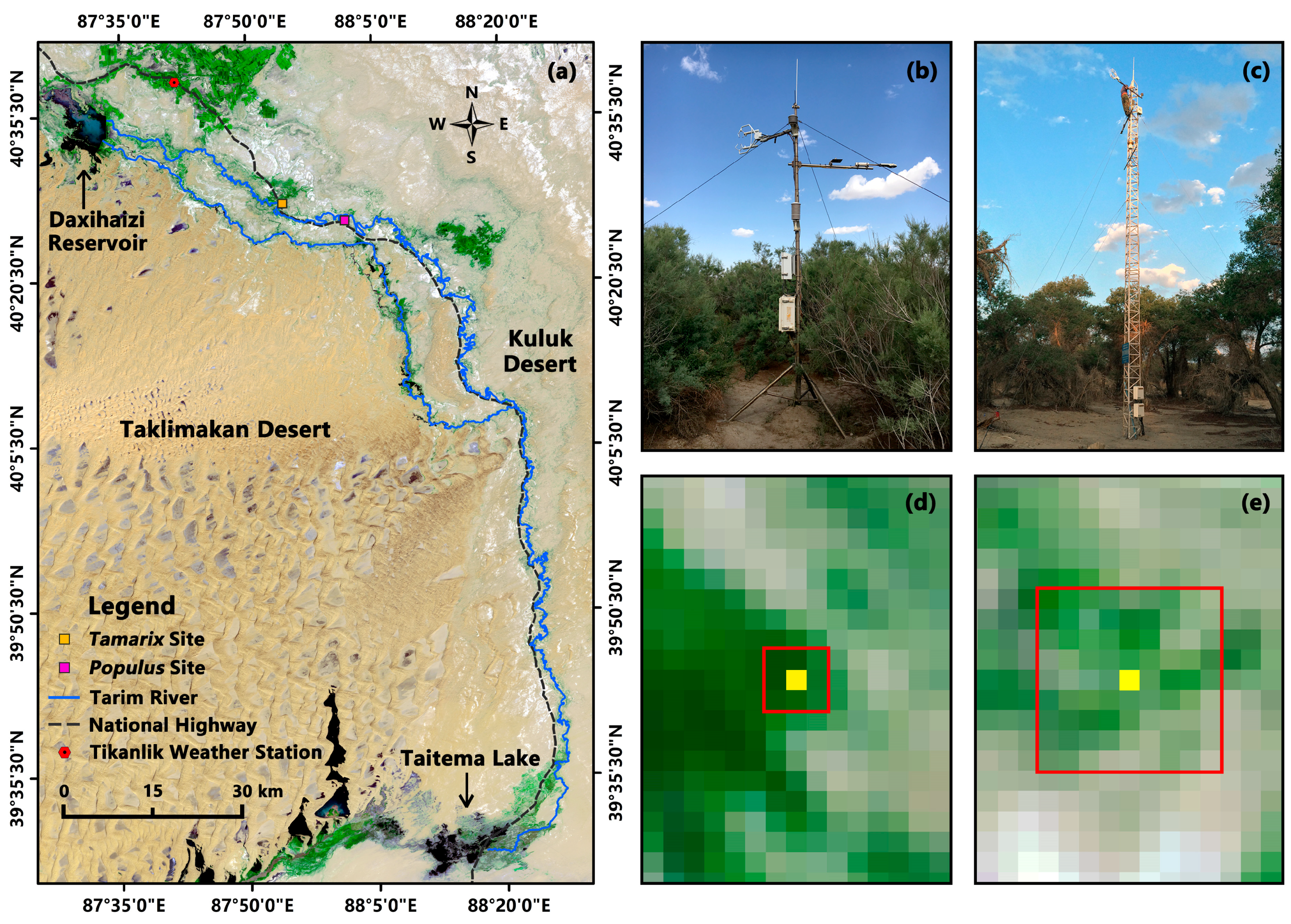
2.2. Site Description

The study area is in the lower reaches of the Tarim River, which flows between the Taklimakan Desert and the Kuluk Desert and stretches from the Daxihaizi Reservoir to the Taitema Lake (Figure 1). The study area has the characteristics of a relatively flat land surface [36] and a hyper-arid climate [37]. According to the meteorological observations from the Tikanlik Weather Station, the average annual temperature is 10.5 °C, the annual precipitation is between 17 and 40 mm, and the potential evaporation is approximately 3000 mm yr⁻¹ [6,37]. The vegetation is sparse and dominated by Tamarix ramosissima (T. ramosissima) and Populus euphratica (P. euphratica), which are typical phreatophytes, and belong to shrub and arbor forests, respectively [21,38]. Due to poor water conditions, the vegetation coverage and species richness of plant communities in the study area are relatively low [11].

According to the difference in vegetation types, we selected two typical sites to carry out this study. One site is dominated by T. ramosissima, and the other is dominated by P. euphratica. In this study, the former was called the Tamarix site, and the latter was called the Populus site.

The Tamarix site (87°54’E, 40°27’N) has a Simpson Diversity Index of 0.71, with a few herbs growing under the T. ramosissima. The height of the vegetation canopy is approximately 2 m, with a vegetation coverage index of 0.65. The LAI measured by the LAI-2250 Plant Canopy Analyzer was 1.15 in July 2013. The soil is generally silty loam, with an approximately 20 cm dry sand covering on the land surface. The groundwater table depth fluctuated between 4.4 and 5.9 m during the observation period.

The Populus site (88°01’E, 40°26’N) has the single vegetation species, with an average canopy height of about 10 m. At the Populus site, the LAI and the vegetation coverage index were 0.57 and 0.47, respectively. The soil from the land surface to a depth of 3 m is silty loam, and it is mainly sand below 3 m. The groundwater table depth ranged from 3.5 to 6.3 m during the observation period.

2.3. Data and Processing

2.3.1. ET Data

The eddy covariance (EC) system was deployed on the flux tower of the Tamarix site and on the flux tower of the Populus site, respectively, to measure the energy and H₂O/CO₂ fluxes. The instruments have been described in detail in [10,11]. The measurements started in June 2011 over the Tamarix site and in June 2013 over the Populus site.

For both EC flux towers, fluctuations in vapor density, virtual air temperature, and wind speed were sampled at a frequency of 10 Hz. In addition, soil heat flux and meteorological data were measured and recorded every 30 min.

We used EC data from the end of April 2013 to the end of October 2018 in this study. For the Tamarix site, data for an extended period (form 29 January 2018 to 31 October 2018) were missing due to the malfunction of instruments. We did not perform gap-filling during the data process.

Raw EC data (10 Hz) were corrected and processed, using the EdiRe software (School of Geosciences, University of Edinburgh). In EdiRe, the correction procedures applied to the raw EC data included spike removal, spectral correction, coordinate rotation correction, sonic virtual temperature correction, lag correction of H₂O/CO₂ relative to the vertical wind component, and WPL density correction. All of the raw EC data were processed to 30 min averages.

The energy balance was forced to close by augmenting both latent and sensible heat fluxes while retaining the observed Bowen ratio [39], and the corrected latent heat flux (LE, W m^–2) was used to calculate half-hourly ET (mm), using Equation (3):

$$ET=\frac{LE}{L\times {\rho }_w}$$

(3)

where $L$ is the latent heat of vaporization of water (2.45 kJ g⁻¹); and ${\rho }_w$ is water density (1 g cm⁻³). Daily ET (mm d⁻¹) was obtained by summing up all of the 48 half-hourly ET for one day. In the calculation process, when the half-hourly ET was negative, it was set to zero.

2.3.2. T_a,m and ET₀ Data

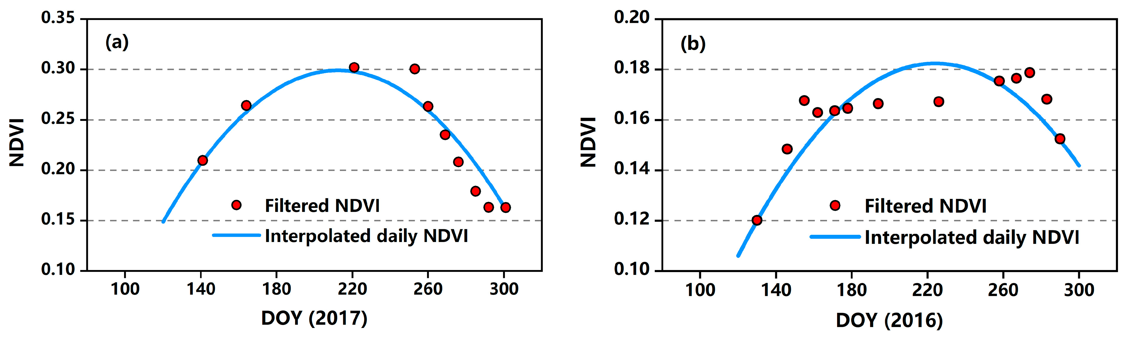
Due to the malfunction of instruments or other errors, the daily meteorological variables measured by both flux towers were missing for some periods. In this study, we used the daily meteorological variables recorded at the Tikanlik Weather Station, which has a distance of approximately 30−40 km from the two study sites (Figure 1). The meteorological variables include mean relative humidity, wind speed, pressure, the actual duration of sunshine, daily maximum air temperature, and daily minimum air temperature. These meteorological data were mainly used to calculate the reference evapotranspiration (ET₀) through the FAO Penman–Monteith approach (Equation (4)) [34]:

$$E{T}_0=\frac{0.408\Delta \left(R_n-G\right)+\mathsf{\gamma }\frac{900}{T+273}{u}_2\left(e_s-e_a\right)}{\Delta +\mathsf{\gamma }\left(1+0.34u_2\right)}$$

(4)

where, $E{T}_0$ is reference evapotranspiration (mm d⁻¹); $R_n$ is the net radiation at the crop surface (MJ m⁻² d⁻¹); $G$ is the soil heat flux density (MJ m⁻² d⁻¹), and it is assumed to be zero on daily time steps; $T$ is mean daily air temperature at 2 m height (°C); $u_2$ is the wind speed at 2 m height (m s⁻¹); $e_s$ is saturation vapor pressure (kPa); $e_a$ is actual vapor pressure (kPa); $e_s-e_a$ is saturation vapor pressure deficit (kPa); $\Delta$ is the slope of vapor pressure curve (kPa °C⁻¹); and $\mathsf{\gamma }$ is psychrometric constant (kPa °C⁻¹). Detailed calculations of the parameters in Equation (4) based on the above meteorological data were presented in [34].

We also calculated ET₀ by using the available daily meteorological variables observed by both flux towers during the study period, respectively, and compared them with the results calculated by using data from the Tikanlik Weather Station. For each site, the comparison results showed a high degree of correlation between ET₀ calculated from these two sets of data (R² = 0.927 for the Tamarix site and R² = 0.934 for the Populus site; data not shown here).

2.3.3. NDVI Data

In this study, we downloaded Landsat 8 L1T scenes covering the 2013–2018 growing season (the growing season of T. ramosissima and P. euphratica is from DOY 121 to DOY 300 in the study area [10,21]) from the USGS GloVis [40]. Although the two study sites are in an overlapping part of two adjacent scenes (paths 141 and 142, row 32), most of the images have a high cloud cover, and only 65 cloud-free images were used in our analysis. To convert the original digital number (DN) values into surface reflectance, we performed radiometric calibration first and then atmospheric correction for all images, using the FLAASH module embedded in ENVI 5.3.1 (Exelis Visual Information Solutions, Boulder, CO, USA). Detailed processing was introduced in [32]. Afterword, the NDVI for each image was determined by using Equation (5) [41]:

$$NDVI=\frac{{\rho }_{NIR}-{\rho }_{Red}}{{\rho }_{NIR}+{\rho }_{Red}}$$

(5)

where ${\rho }_{NIR}$ and ${\rho }_{Red}$ are the reflectance of the near-infrared band and red band, respectively. Finally, the NDVI time-series was constructed by stacking all the NDVI images.

Furthermore, we used the Savitzky–Golay filter technique [42,43] to smooth the NDVI time-series, in order to minimize the perturbations due to anisotropic bidirectional effects, atmospheric instability, and system failure [44,45,46]. This method was selected because it performs better than other methods for NDVI noise-reduction in the arid ecosystems of Northwestern China [45]. The half-width of the smoothing window and the degree of the smoothing polynomial must be determined according to the NDVI observations when using this approach to smooth NDVI time-series. A smoother filtered NDVI time-series is usually generated by a higher half-width value of the smoothing window. It is typically set to an integer between 2 to 4 for the degree of the smoothing polynomial [43]. In this study, both of them were set as three.

Subsequently, to compare these ERSETMs comprehensively, the NDVI for each day throughout the whole growing season was required. Therefore, we interpolated the filtered NDVI of the growing season from 2013 to 2018 for both sites. The interpolation was performed on a pixel basis and included the following steps primarily: (1) The filtered NDVI was fitted to DOY by using a quadratic parabola; and (2) daily NDVI was estimated by using the fitted quadratic parabola function. In particular, the quadratic function was forced to pass through the first and last data points during the fitting process, in order to achieve a better interpolated daily NDVI time-series.

Finally, for the interpolated and the filtered NDVI time-series, the NDVI values of the pixels covering the footprint area of each flux tower were extracted and spatially averaged for each day. The averaged NDVI values were used for the analyses of each site. As an example, Figure 2a shows the two NDVI time-series for the 2017 growing season of the Tamarix site, and Figure 2b displays both NDVI time-series for the 2016 growing season of the Populus site.

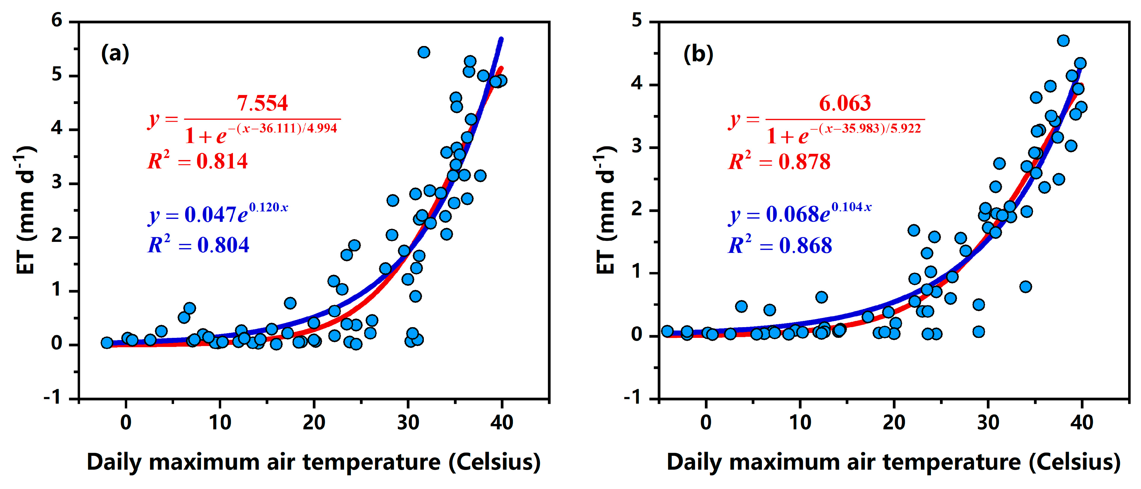
2.4. Calibration of ERSETMs

In this study, we calibrated these ERSETMs in Table 1 for the Tamarix site and the Populus site separately. There are a few things to note concerning the model calibration. Initially, due to the high degree of correlation between T_s,n and T_a,m [47,48], the T_s,n in the Scott-2008 model and the Bunting-2014 model was replaced with the T_a,m following [12]. Furthermore, because the comparison of these ERSETMs in this study was made for the two study sites separately, we used the VI dataset of each site directly and did not scale them in the calibration of the Nagler-2005a model, Nagler-2005b model, Bunting-2014 model, and the Nagler-2009 model, following [16]. Additionally, in the calibration of the Nagler-2009 model and the Glenn-2015 model, ET₀ computed using the Penman–Monteith equation was used rather than ET₀ calculated from the Blaney–Criddle formula, since the former is preferred and considers the meteorological factors influencing ET more comprehensively [49,50,51]. Finally, LAI in the Yuan-2016 model for the Tamarix site ($LA{I}_T$) and the Populus site ($LA{I}_P$) was estimated based on the relationship between LAI and NDVI in the lower Tarim River [52]:

$$LA{I}_T=0.216NDV{I}^2+5.744NDVI-0.356$$

(6)

$$LA{I}_P=9.295NDV{I}^2+1.124NDVI-0.115$$

(7)

Therefore, we used the daily ET, T_a,m, and ET₀ estimated by using the Penman–Monteith equation, and the NDVI data to calibrate these ERSETMs.

We partitioned the dataset into two parts for each site, with approximately 80% and 20% of the data. The former was used as the calibration dataset and the latter as the validation dataset. Taking into account the relative integrity of the observed daily ET and the filtered NDVI, we used the 2017 data of the Tamarix site (9 samples) and the 2016 data of the Populus site (11 samples) as the validation dataset for the Tamarix site and the Populus site, respectively, and data from the other years (41 samples for the Tamarix site and 38 samples for the Populus site) were used as their respective calibration dataset.

We calibrated the eight ERSETMs by using the calibration dataset of the Tamarix site and the Populus site, respectively. The calibration process was conducted by the regression analysis, using OriginPro 2020 (Learning Edition) (OriginLab Corporation, Northampton, MA, USA). A nonlinear curve fit program embedded in OriginPro 2020 was used to determine the empirical parameters of each model. However, the calibration steps of the temperature-based models and the ET₀-based models are different.

For the calibration of the temperature-based models, we referred to the method presented in [12,15]. Primarily, the parameter b in the relationship between ET and VI was determined for the Tamarix site and the Populus site, respectively. In this study, we used 0.221 and 9.598 for parameter b in the temperature-based models of the two study sites, respectively. These values were from [32], in which the Nagler-2013 model has been calibrated for the Tamarix site and the Populus site separately, using data from both the growing season and the non-growing season. Therefore, these values can better express the relationships between ET and VI for both sites. Moreover, the relevant parameters for describing the relationships between ET and T_a,m were determined by fitting ET with T_a,m using a logistic curve following [15] and using an exponential relationship following [16,17], respectively (Figure 3). Notably, data for the non-growing season were also included in Figure 3. In this study, the parameter c in the Nagler-2005a model was determined as 20 for both sites (parameter c represents the threshold temperature for vegetation growth, and temperatures below about c °C supported negligible ET [12]); parameters c, d, and e in the Nagler-2005b model were determined as 7.554, 36.111, and 4.994 for the Tamarix site and as 6.063, 35.983, and 5.922 for the Populus site; parameter d in the Scott-2008 model and parameter c in the Bunting-2014 model were determined as 0.120 for the Tamarix site and as 0.104 for the Populus site. Finally, the other parameters of the temperature-based models were determined by fitting the corresponding model equation to the calibration data while maintaining the above-determined parameters.

Nevertheless, the calibration of the ET₀-based models is relatively simple. For their calibrations, the corresponding model equation was directly fitted to the calibration data of the two study sites, respectively. Notably, parameter b in the Nagler-2013 model of the two study sites also used the values as mentioned above.

In the process of nonlinear curve fit, each equation was subjected to statistical verification through the coefficient of determination (R²), reduced chi-square values, and P-values for the regression coefficient.

Table 2. Calibration results of the eight ERSETMs for the two study sites.

Models	Tamarix Site						Populus Site
	a	b	c	d	e	f	a	b	c	d	e	f
Nagler-2005a	4.373	0.221	20.00	−0.046			0.236	9.598	20.00	0.092
Nagler-2005b	17.802	0.221	7.554	36.111	4.994	0.224	1.203	9.598	6.063	35.983	5.922	0.197
Scott-2008	67.234	0.221	0.038	0.120	−2.742		8.456	9.598	0.054	0.104	−6.076
Bunting-2014	0.856	0.221	0.120	0.198			0.080	9.598	0.104	0.212
Nagler-2009	2.354						2.999
Nagler-2013	16.774	0.221	0.306				2.309	9.598	1.334
Glenn-2015	4.941	1.086	0.335				3.675	0.594	0.245
Yuan-2016	0.543						1.512

shows the calibration results of these ERSETMs compared in this study.

2.5. Evaluation of Model Performance

The performance of these ERSETMs at each site was evaluated by using the following metrics: determination coefficient (R²); Nash–Sutcliffe efficiency (NSE); root mean square error (RMSE); mean absolute error (MAE); and maximum error (MaxError). Researchers commonly use these metrics in evaluating the reliability of ET models [53,54,55,56,57,58].

$$R^2=\frac{{\left[{{\displaystyle \sum }}_{i=1}^n\left(E{T}_{s,i}-{\phi }_0\right)\left(E{T}_{o,i}-{\mu }_0\right)\right]}^2}{{{\displaystyle \sum }}_{i=1}^n{\left(E{T}_{s,i}-{\phi }_0\right)}^2{{\displaystyle \sum }}_{i=1}^n{\left(E{T}_{o,i}-{\mu }_0\right)}^2}$$

(8)

$$NSE=1-\frac{{{\displaystyle \sum }}_{i=1}^n{\left(E{T}_{s,i}-E{T}_{o,i}\right)}^2}{{{\displaystyle \sum }}_{i=1}^n{\left(E{T}_{o,i}-{\mu }_0\right)}^2}$$

(9)

$$RMSE=\sqrt{\frac{{{\displaystyle \sum }}_{i=1}^n{\left(E{T}_{s,i}-E{T}_{o,i}\right)}^2}{n}}$$

(10)

$$MAE=\frac{1}{n}{\displaystyle \sum }_{i=1}^n\left|E{T}_{s,i}-E{T}_{o,i}\right|$$

(11)

$$MaxError=\max \left|E{T}_{s,i}-E{T}_{o,i}\right|$$

(12)

where $E{T}_{o,i}$ and $E{T}_{s,i}$ are observed and simulated ET, respectively, during day I; ${\mu }_0$ is the mean of observed ET values; ${\phi }_0$ is the mean of simulated ET values; and n is the total number of observation days.

3. Results

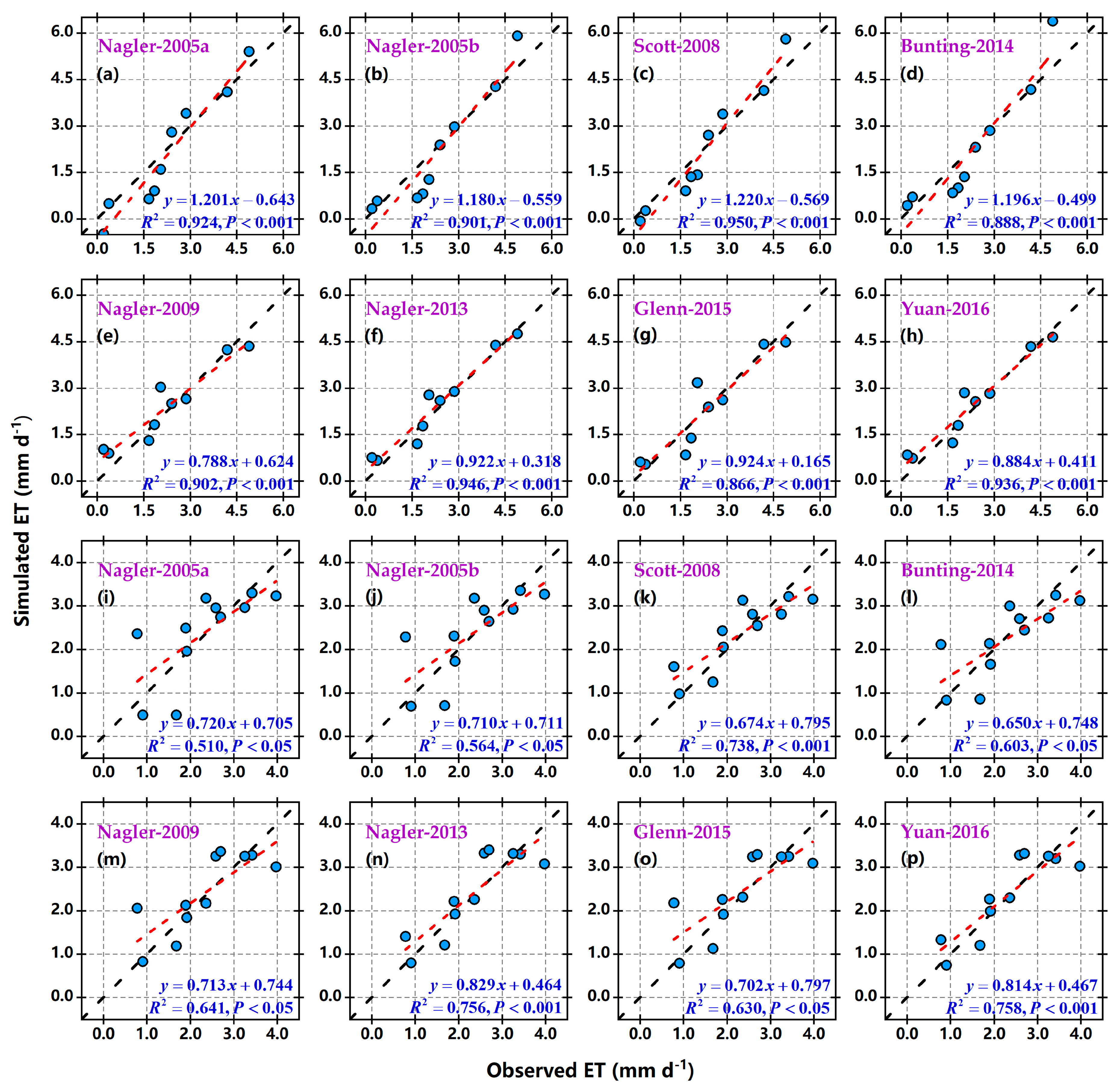
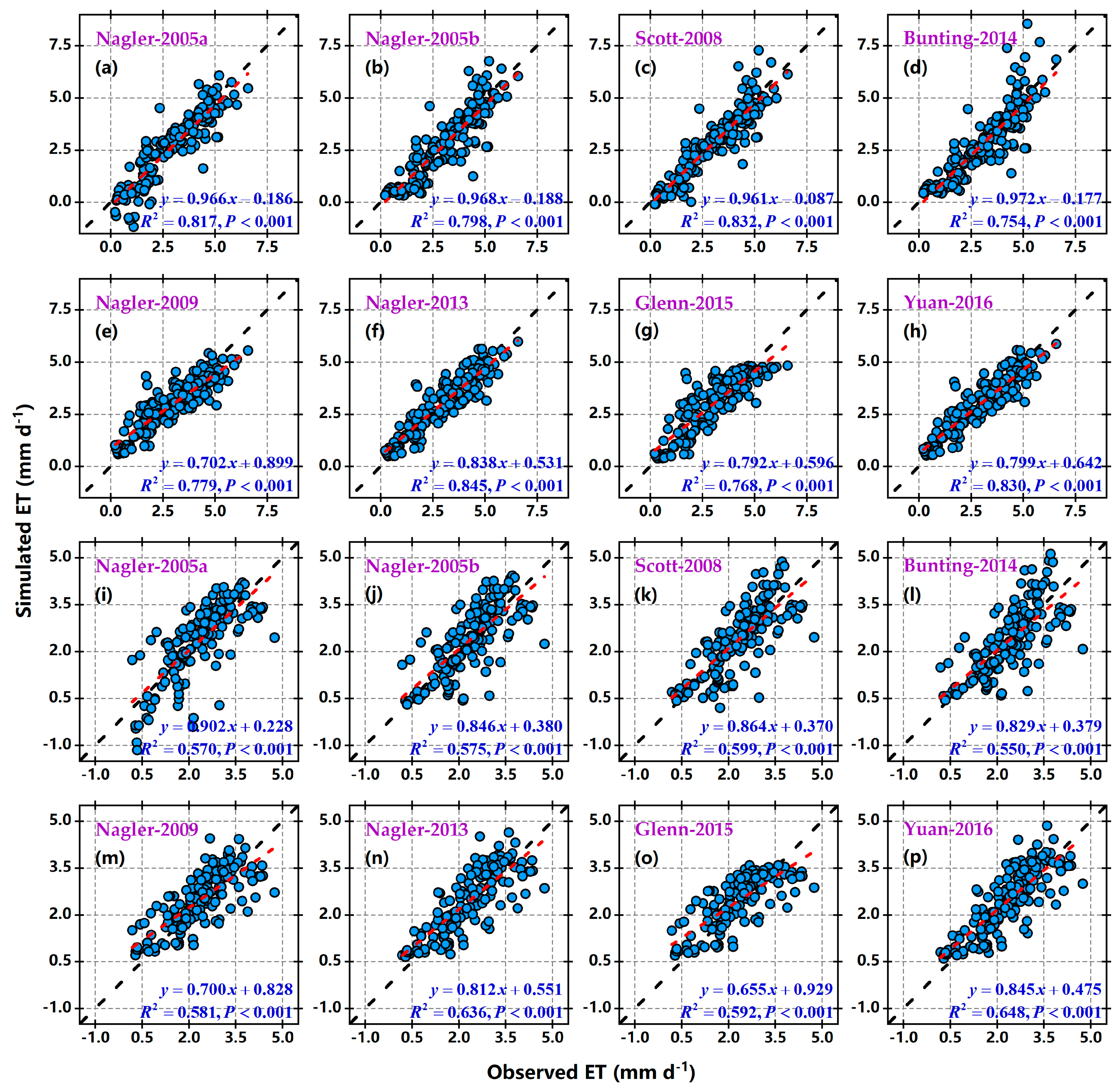
3.1. Validation of ERSETMs

Figure 4 shows the validation results of the eight ERSETMs for the Tamarix site (Figure 4a–h) and the Populus site (Figure 4i–p). Generally, the simulated ET agreed well with the observed ones for both sites. The eight ERSETMs explained 86.6%–95.0% and 51.0%–75.8% of ET variability over the validation dataset of the two study sites, respectively. However, the performance of the eight ERSETMs showed substantial differences between the two sites.

3.2. Comparison of Estimates from ERSETMs

3.2.1. Statistical Performance of ERSETMs

Primarily, the validation results of the eight ERSETMs for both sites (Figure 4) indicated appropriate agreements between the observed and simulated ET values. The Scott-2008 model produced the highest determination coefficient for the Tamarix site (R² = 0.950), followed by the Nagler-2013 model (R² = 0.946) and the Yuan-2016 model (R² = 0.936). Compared with the above three models, the other models presented relatively low R² values, varying from 0.866 to 0.924. Likewise, there was a better performance of the Yuan-2016 model, the Nagler-2013 model, and the Scott-2008 model for the Populus site, and the R² values of these three models were 0.758, 0.756, and 0.738 respectively. Notably, the eight ERSETMs performed significantly better at the Tamarix site than at the Populus site.

Moreover, Figure 5 depicts the comparison between the observed and simulated ET for each day throughout the 2017 growing season of the Tamarix site (Figure 5a–h) and each day throughout the 2016 growing season of the Populus site (Figure 5i–p). Overall, the data points were reasonably close to the 1:1 lines, with R² values varying from 0.754 to 0.845 for the Tamarix site and ranging from 0.550 to 0.648 for the Populus site. As with the comparison of validation results, better results were achieved for the Scott-2008 model, the Nagler-2013 model, and the Yuan-2016 model for both sites. The other models demonstrated poor performance, with relatively low R² values for both sites. In addition, all models showed better performance at the Tamarix site than that at the Populus site, and the Nagler-2005a model produced some negative daily ET values at both sites (Figure 5a,i).

Ultimately,

Table 3. Statistical performance of the eight ERSETMs for the validation dataset of the Tamarix site and the Populus site. The total number of observations was 9 for the Tamarix site and 11 for the Populus site. The Nash–Sutcliffe efficiency (NSE) is unitless. The root mean square error (RMSE), mean absolute error (MAE), and the maximum error (MaxError) are in millimeters per day. The greener the color of the cells, the better the model performs.

Models	NSE		RMSE		MAE		MaxError
	Tamarix	Populus	Tamarix	Populus	Tamarix	Populus	Tamarix	Populus
Nagler-2005a	0.826	0.421	0.611	0.730	0.529	0.562	1.034	1.574
Nagler-2005b	0.805	0.525	0.647	0.662	0.480	0.508	1.040	1.496
Scott-2008	0.871	0.731	0.525	0.498	0.449	0.417	0.904	0.820
Bunting-2014	0.780	0.595	0.687	0.611	0.502	0.482	1.482	1.327
Nagler-2009	0.878	0.626	0.511	0.587	0.399	0.435	0.975	1.271
Nagler-2013	0.936	0.744	0.371	0.486	0.295	0.377	0.727	0.901
Glenn-2015	0.862	0.609	0.543	0.600	0.431	0.436	1.131	1.390
Yuan-2016	0.923	0.752	0.407	0.478	0.322	0.380	0.805	0.950

and

Table 4. Statistical performance of the eight ERSETMs for daily ET throughout the 2017 growing season of the Tamarix site and daily ET throughout the 2016 growing season of the Populus site. The total number of observations was 170 for the Tamarix site and 150 for the Populus site. The NSE is unitless. The RMSE, MAE, and the MaxError are in millimeters per day. The greener the color of the cells, the better the model performs.

Models	NSE		RMSE		MAE		MaxError
	Tamarix	Populus	Tamarix	Populus	Tamarix	Populus	Tamarix	Populus
Nagler-2005a	0.753	0.376	0.755	0.776	0.552	0.593	2.818	2.696
Nagler-2005b	0.726	0.447	0.796	0.731	0.592	0.561	3.191	2.507
Scott-2008	0.792	0.480	0.692	0.709	0.504	0.551	2.608	2.449
Bunting-2014	0.661	0.408	0.885	0.756	0.644	0.582	3.346	2.669
Nagler-2009	0.770	0.543	0.728	0.665	0.576	0.514	2.622	2.035
Nagler-2013	0.845	0.576	0.599	0.640	0.453	0.504	2.228	1.900
Glenn-2015	0.765	0.573	0.737	0.642	0.569	0.499	2.764	1.881
Yuan-2016	0.829	0.576	0.628	0.640	0.481	0.508	2.351	1.754

present the statistical performance of the eight ERSETMs for the above two datasets, respectively. In general, for both sites, the ET₀-based models performed better than the temperature-based models, which had a relatively lower NSE and relatively higher RMSE, MAE, and MaxError values. In the ET₀-based models, the Nagler-2013 model and the Yuan-2016 model yielded better performance. Similarly, the eight ERSETMs showed relatively better performance at the Tamarix site than at the Populus site, and the higher NSE values were achieved at the Tamarix site.

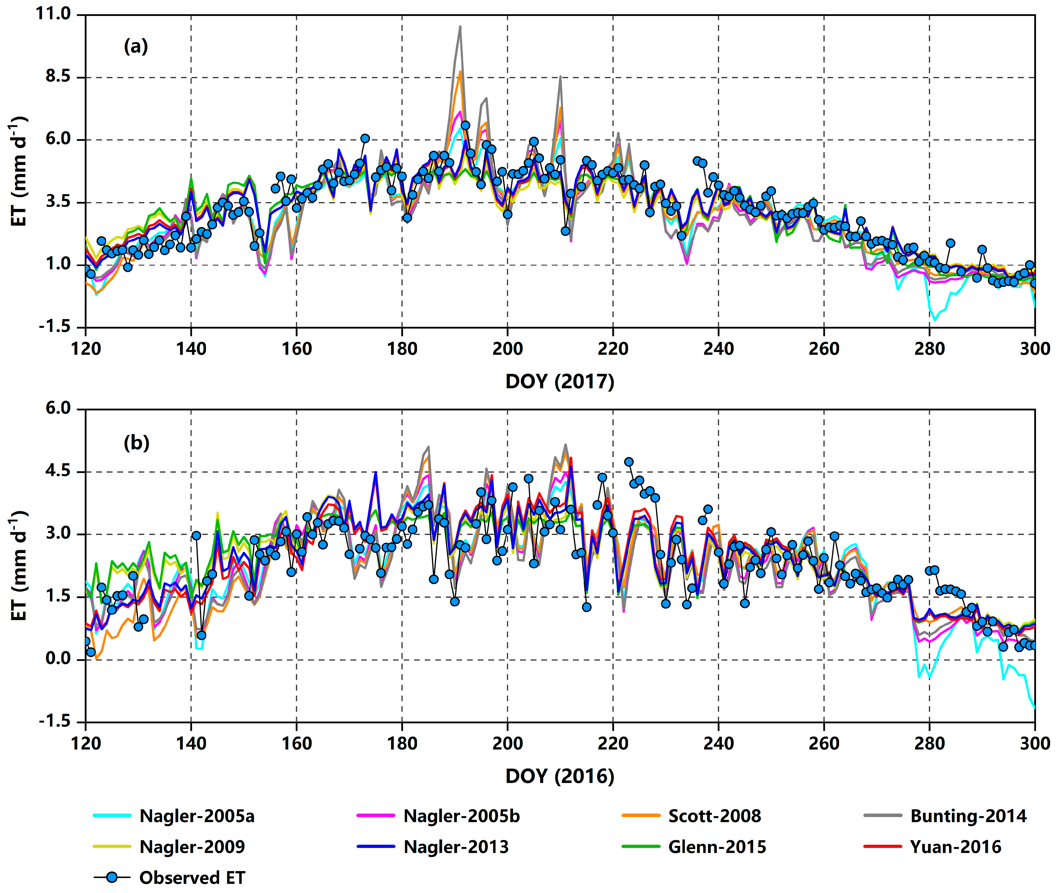
3.2.2. Performance in Daily Variations

Figure 6 displays the daily variations of the observed and simulated daily ET for the 2017 growing season of the Tamarix site and the 2016 growing season of the Populus site. All eight ERSETMs captured the variation process of daily ET, which increased continuously during the first half of the growing season and decreased gradually during the second half of the growing season. However, there were some differences between the models. Compared with the ET₀-based models, the temperature-based models showed a relatively worse performance. The Nagler-2005a model provided some negative daily ET values for both sites at the end of the growing season. In addition, the Scott-2008 model and the Bunting-2014 model produced some extreme values from DOY 180 to DOY 240, especially for the Tamarix site. As a whole, the Nagler-2013 model and the Yuan-2016 model had better performance and provided a very consistent variation process with the observed daily ET for both sites.

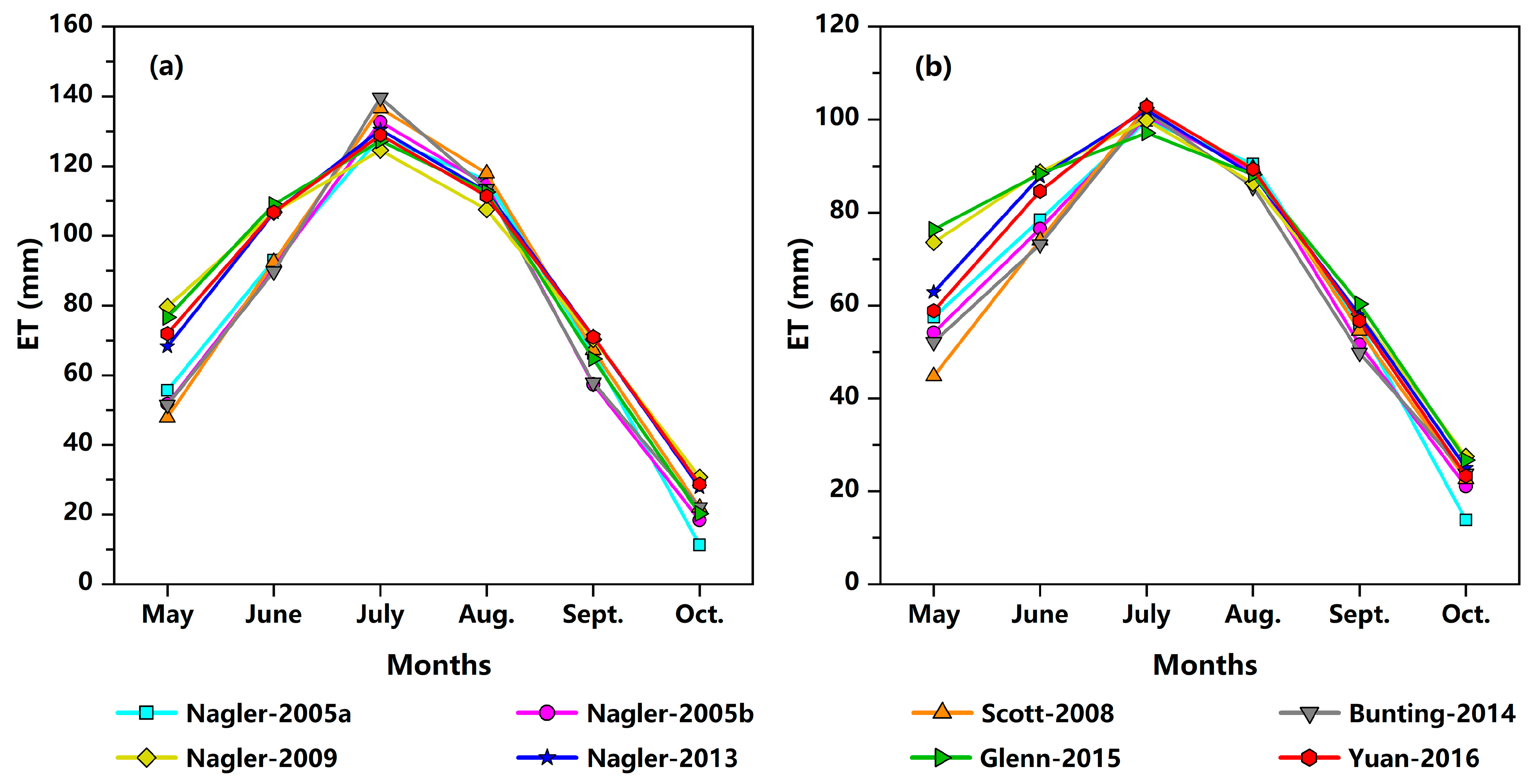
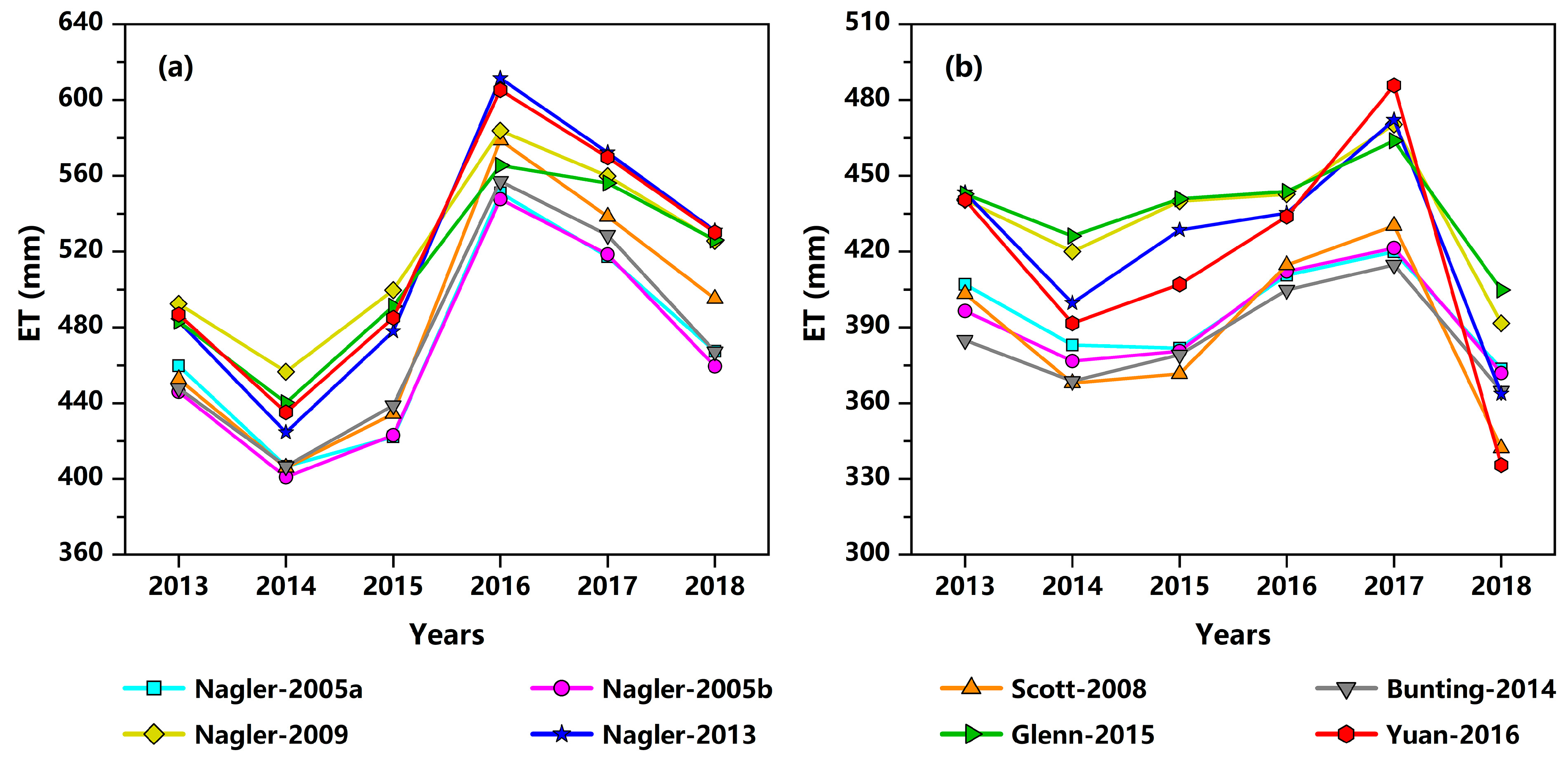
3.2.3. Differences in Monthly and Seasonal Scales

Figure 7 depicts the variability of the mean monthly ET for the growing season from 2013 to 2018 estimated by the eight ERSETMs. All of the eight ERSETMs captured the variation characteristics of the monthly ET and revealed a similar monthly variation, which presented a process of increasing first and then decreasing with the maximum value in July and minimum value in October. However, there were substantial differences in the monthly ET estimation among these models. On the whole, the differences were relatively significant in May, June, and October. Both sites showed that the ET₀-based models achieved larger mean monthly ET values than the temperature-based models in May and June. Notably, compared with the other models, the Nagler-2005a model presented the smallest mean monthly ET values for October because there were some negative daily ET values in October estimated by this model (Figure 5a,i and Figure 6).

The mean ET of the growing season from 2013 to 2018 revealed significant differences among the eight ERSETMs (Figure 8). The ET₀-based models showed the higher mean ET values of the growing season, which ranged from 510.41 to 519.65 mm for the Tamarix site and from 415.70 to 437.05 mm for the Populus site, respectively. However, the mean ET of the growing season estimated by the temperature-based models ranged from 465.93 to 484.23 mm for the Tamarix site and from 386.22 to 396.01 mm for the Populus site, respectively. Similarly, the interannual variability of the ET for the growing season from 2013 to 2018 also demonstrated considerable differences among the eight ERSETMs (Figure 9). The growing season ET for all years estimated by the ET₀-based models was generally higher than that estimated by the temperature-based models, and this result mainly due to the relatively sizeable monthly ET values achieved by the ET₀-based models in May and June (Figure 7).

4. Discussion

4.1. Primary Sources of Different Performance Across ERSETMs

4.1.1. Characterization of Meteorological Conditions

The eight ERSETMs compared in this study used T_a,m, T_s,n, and ET₀ to characterize the meteorological conditions. Generally, our results showed better performance of the ET₀-based models compared to the temperature-based models (Figure 4 and Figure 5; Table 3 and Table 4). ET is affected by a variety of meteorological factors, including wind speed, solar radiation, and air humidity [59]. Although air temperature is an indirect reflection of solar radiation, water molecules could not move into the atmosphere if the wind is absent or if the atmosphere has already been saturated with humidity [59]. Therefore, all meteorological factors affecting ET processes should be considered as comprehensively as possible in these ERSETMs. Similarly, Yuan et al. [11] found that ET was significantly correlated with ET₀ on an hourly scale in the study area, but was not significantly correlated with any of the main meteorological factors, including the air temperature. ET₀ computed using the Penman–Monteith equation [34] in this study takes all the main variables affecting ET into consideration. However, the Blaney–Criddle formula used in the initial construction of the Nagler-2009 model and the Glenn-2015 model is a temperature-dominated method. Studies indicated that the Penman–Monteith method outperformed other ET₀ models [60] and has been regarded as the standard model for ET₀ computation and the calibration of other empirical ET₀ models [61,62,63]. To sum up, ET₀ estimated using the Penman–Monteith equation is a better characterization for the meteorological conditions in these ERSETMs.

4.1.2. Effects of Vegetation Factors

By and large, all eight ERSETMs performed relatively better at the Tamarix site than at the Populus site for both the validation dataset and the daily estimates throughout the whole growing season (Figure 4 and Figure 5; Table 3 and Table 4). This result appears to be associated with the coverage of vegetation and the NDVI data quality. On the one hand, compared with the Tamarix site, the Populus site has lower vegetation coverage (Figure 1d,e). Studies also showed that MODIS ET presented relatively considerable uncertainty in sparse vegetation areas [1,64]. Similarly, Yang et al. [65] reported that the TSEB (Two-Source Energy Balance) model showed significant uncertainties for ET partitioning, particularly over sparse vegetation regions. On the other hand, the NDVI data quality of the Populus site was relatively more inferior than that of the Tamarix site (Figure 2). Similarly, studies showed that ET estimated from the SEBAL algorithm was most sensitive to the vegetation index (NDVI) [66], particularly in areas of sparse canopy cover [67]. In addition, the difference in monthly ET estimated from the eight ERSETMs for both sites was larger in May, June, and October; however, it was relatively smaller from July to September (Figure 7). Therefore, the characterizations of vegetation factors specifically affect the ET estimation from these ERSETMs, and the requisite attention may be needed for ET estimation in sparse vegetation areas using these ERSETMs.

Furthermore, the Nagler-2009 model and the Yuan-2016 model are substantially the same. The distinction between the two models is the characterization of the vegetation factors: The former used NDVI, while the latter used LAI (Table 1). Our results demonstrated that the Yuan-2016 model presented better performance than the Nagler-2009 model for both sites. This result suggests that LAI seems to be a better characterization of vegetation factors than NDVI for this specific model structure. LAI is directly correlated with the light absorbed by the vegetation foliage and has an essential effect on the photosynthetic activity and ET processes [68]. Similarly, studies also reported that LAI controlled the spatial variations of ET [11] and the seasonal variations of T/ET [69,70] in the arid ecosystems of Northwestern China.

4.1.3. Effects of Model Structures

In summary, the eight ERSETMs contain four types of model structures. The temperature-based models and ET₀-based models include two model structures, respectively (

Table 5. Model structures of the eight ERSETMs compared in this study.

Categories	Model Structures	Models
Temperature-based models	MS1: $ET=f\left(VI\right)+f\left(T\right)$	Scott-2008
	MS2: $ET=f\left(VI\right)\times f\left(T\right)$	Nagler-2005a; Nagler-2005b; Bunting-2014
ET0-based models	MS3: $ET=f\left(VI\right)\times E{T}_0$	Nagler-2009; Nagler-2013; Yuan-2016
	MS4: $ET=f\left(VI\times E{T}_0\right)$	Glenn-2015

In the model structures, the items $f\left(VI\right)$, $f\left(T\right)$, and $f\left(VI\times E{T}_0\right)$ represent a specific function regarding vegetation index, temperature, and $VI\times E{T}_0$, respectively. $E{T}_0$ is the reference evapotranspiration, and $T$ represents the daily maximum air temperature (T_a,m) or the nighttime land-surface temperature (T_s,n).

).

Although the expressions of meteorological conditions and vegetation factors are the same in the Scott-2008 model and the Bunting-2014 model (Table 1), they have different model structures (Table 5). In terms of the combination of meteorological conditions and vegetation factors, the Scott-2008 model used the additive approach, while the Bunting-2014 model adopted the multiplicative approach (Table 5). However, the performance of the Scott-2008 model was generally better than that of the other three temperature-based models (Figure 4 and Figure 5; Table 3 and Table 4). Similarly, in the original construction of the Scott-2008 model, they reported that the calibration results were improved by changing the model structure of the Nagler-2005b model (MS2) to the one they used (MS1) [16]. Thus, these results indicate that the MS1 seems to be relatively more appropriate for the temperature-based models.

Compared with the temperature-based models, the ET₀-based models achieved better estimating results. Overall, the Nagler-2013 model and the Yuan-2016 model were superior to the other six models. The structure of the two models (MS3) is similar to the crop coefficient method (Equation (1)). However, the $K_c$ in the crop coefficient method was substituted by using different functions of vegetation indices in the Nagler-2013 model and the Yuan-2016 model. The former used an exponential function of NDVI or EVI modified from the Beer–Lambert Law, while the latter used a linear function of LAI (Table 1). Therefore, these results imply that the MS3 may be a better model structure for the construction of ERSETMs in arid riparian ecosystems.

4.2. Considerations for the Applications of ERSETMs

From an application perspective, as reported by Karimi and Bastiaanssen [71], the absence of regional-scale validation of ET estimation is one of the drawbacks in defining the reliability of remotely sensed ET products. However, these ERSETMs extrapolate ET observed or estimated at the site scale to regional scales based on the empirical relationship constructed at the site scale, and they are different from the commonly used ET algorithms based on the energy-balance equation. For these ERSETMs, their estimation accuracy at the site scale is the basis for accurate ET estimation at the regional scales and has a direct influence on the regional-scale ET estimation [32]. Therefore, the comparison of model performance at the site scale is meaningful for their application for regional-scale ET estimation.

By comparing the performance of the eight ERSETMs, we found that the Nagler-2013 model and the Yuan-2016 model outperformed the other models. Furthermore, we provided model parameters of the Nagler-2013 model and the Yuan-2016 model for the main vegetation types (Tamarix ramosissima and Populus euphratica) in arid riparian ecosystems. Our findings are meritorious for the selection of ERSETMs and ET estimation of Tamarix ramosissima and Populus euphratica in similar ecosystems. Additionally, these results also have potential application value for weather and climate modeling [2], ecosystem and environmental assessment [23,72], and sustainable water resources management [73,74] in arid regions.

Notably, the Nagler-2013 model and the Yuan-2016 model have their advantages and disadvantages when applied to regional-scale ET estimation. The Nagler-2013 model uses readily available NDVI or EVI, but there are more model parameters, while the Yuan-2016 model has fewer model parameters, but the collection of measured LAI data is relatively tricky. However, the development of global LAI products [68,75,76,77] may provide a specific application foundation for the Yuan-2016 model. As mentioned in Section 4.1.2, characterization indicators of vegetation factors and their data quality also have an impact on the performance of ERSETMs. Therefore, in practical applications, the availability of remote-sensing data and their quality should be considered comprehensively in selecting an appropriate model between the two models.

5. Conclusions

In this study, we compared eight ERSETMs, using ET measurements of two typical sites in an arid riparian ecosystem of Northwestern China. The results showed that the Nagler-2013 model and the Yuan-2016 model outperformed the other models. The differences in model structures and characterization of both meteorological conditions and vegetation factors were the primary sources of different model performance. For the characterization of meteorological conditions in these ERSETMs, the reference evapotranspiration (ET₀) estimated by using the Penman–Monteith equation was more appropriate than the daily maximum air temperature. The characterization indicators of vegetation factors and their data quality have a specific influence on model performance. The better model structure for constructing ERSETMs in arid riparian ecosystems was to replace $K_c$ in the crop coefficient method, using an appropriate function of vegetation indices. Our findings provide useful information for choosing models and obtaining accurate ET estimation in arid regions.

References

1. Wang, S.; Pan, M.; Mu, Q.; Shi, X.; Mao, J.; Brümmer, C.; Jassal, R.S.; Krishnan, P.; Li, J.; Black, T.A. Comparing Evapotranspiration from Eddy Covariance Measurements, Water Budgets, Remote Sensing, and Land Surface Models over Canada. J. Hydrometeorol. 2015, 16, 1540–1560. [Google Scholar] [CrossRef] [Green Version]
2. Wang, K.; Dickinson, R.E. A review of global terrestrial evapotranspiration: Observation, modeling, climatology, and climatic variability. Rev. Geophys. 2012, 50, RG2005. [Google Scholar] [CrossRef]
3. Cleverly, J.R.; Dahm, C.N.; Thibault, J.R.; Mcdonnell, D.E.; Coonrod, J.E.A. Riparian ecohydrology: Regulation of water flux from the ground to the atmosphere in the Middle Rio Grande, New Mexico. Hydrol. Process. 2006, 20, 3207–3225. [Google Scholar] [CrossRef] [Green Version]
4. Falkenmark, M.; Rockström, J. Balancing Water for Humans and Nature: The New Approach in Ecohydrology; Earthscan: London and Sterling, UK, 2004; pp. 1–247. [Google Scholar]
5. Glenn, E.P.; Nagler, P.L.; Shafroth, P.B.; Jarchow, C.J. Effectiveness of environmental flows for riparian restoration in arid regions: A tale of four rivers. Ecol. Eng. 2017, 106, 695–703. [Google Scholar] [CrossRef]
6. Chen, Y.N.; Chen, Y.P.; Xu, C.C.; Ye, Z.X.; Li, Z.Q.; Zhu, C.G.; Ma, X.D. Effects of ecological water conveyance on groundwater dynamics and riparian vegetation in the lower reaches of Tarim River, China. Hydrol. Process. 2009, 24, 170–177. [Google Scholar] [CrossRef]
7. Glenn, E.P.; Nagler, P.L.; Huete, A.R. Vegetation index methods for estimating evapotranspiration by remote sensing. Surv. Geophys. 2010, 31, 531–555. [Google Scholar] [CrossRef]
8. Eamus, D.; Zolfaghar, S.; Villalobos-Vega, R.; Cleverly, J.; Huete, A. Groundwater-dependent ecosystems: Recent insights from satellite and field-based studies. Hydrol. Earth Syst. Sci. 2015, 19, 4229–4256. [Google Scholar] [CrossRef] [Green Version]
9. Nouri, H.; Beecham, S.; Anderson, S.; Hassanli, A.M.; Kazemi, F. Remote sensing techniques for predicting evapotranspiration from mixed vegetated surfaces. Urban Water J. 2014, 12, 380–393. [Google Scholar] [CrossRef]
10. Yuan, G.; Zhang, P.; Shao, M.; Luo, Y.; Zhu, X. Energy and water exchanges over a riparian Tamarix spp. stand in the lower Tarim River basin under a hyper-arid climate. Agric. For. Meteorol. 2014, 194, 144–154. [Google Scholar] [CrossRef] [Green Version]
11. Yuan, G.; Luo, Y.; Shao, M.; Zhang, P.; Zhu, X. Evapotranspiration and its main controlling mechanism over the desert riparian forests in the lower Tarim River Basin. Sci. China Earth Sci. 2015, 58, 1–11. [Google Scholar] [CrossRef]
12. Nagler, P.L.; Cleverly, J.; Glenn, E.; Lampkin, D.; Huete, A.; Wan, Z. Predicting riparian evapotranspiration from MODIS vegetation indices and meteorological data. Rem. Sens. Environ. 2005, 94, 17–30. [Google Scholar] [CrossRef]
13. Orellana, F.; Verma, P.; Loheide, S.P.; Daly, E. Monitoring and modeling water-vegetation interactions in groundwater-dependent ecosystems. Rev. Geophys. 2012, 50. [Google Scholar] [CrossRef]
14. Wang, P.; Niu, G.-Y.; Fang, Y.-H.; Wu, R.-J.; Yu, J.-J.; Yuan, G.-F.; Pozdniakov, S.P.; Scott, R.L. Implementing Dynamic Root Optimization in Noah-MP for Simulating Phreatophytic Root Water Uptake. Water Resour. Res. 2018, 54, 1560–1575. [Google Scholar] [CrossRef] [Green Version]
15. Nagler, P.L.; Scott, R.L.; Westenburg, C.; Cleverly, J.R.; Glenn, E.P.; Huete, A.R. Evapotranspiration on western US rivers estimated using the Enhanced Vegetation Index from MODIS and data from eddy covariance and Bowen ratio flux towers. Remote Sens. Environ. 2005, 97, 337–351. [Google Scholar] [CrossRef]
16. Scott, R.L.; Cable, W.L.; Huxman, T.E.; Nagler, P.L.; Hernandez, M.; Goodrich, D.C. Multiyear riparian evapotranspiration and groundwater use for a semiarid watershed. J. Arid Environ. 2008, 72, 1232–1246. [Google Scholar] [CrossRef]
17. Bunting, D.P.; Kurc, S.A.; Glenn, E.P.; Nagler, P.L.; Scott, R.L. Insights for empirically modeling evapotranspiration influenced by riparian and upland vegetation in semiarid regions. J. Arid Environ. 2014, 111, 42–52. [Google Scholar] [CrossRef]
18. Nagler, P.; Morino, K.; Murray, R.S.; Osterberg, J.; Glenn, E. An Empirical Algorithm for Estimating Agricultural and Riparian Evapotranspiration Using MODIS Enhanced Vegetation Index and Ground Measurements of ET. I. Description of Method. Remote Sens. 2009, 1, 1273–1297. [Google Scholar] [CrossRef] [Green Version]
19. Nagler, P.L.; Glenn, E.P.; Nguyen, U.; Scott, R.L.; Doody, T. Estimating riparian and agricultural actual evapotranspiration by reference evapotranspiration and MODIS enhanced vegetation index. Remote Sens. 2013, 5, 3849–3871. [Google Scholar] [CrossRef] [Green Version]
20. Glenn, E.P.; Scott, R.L.; Nguyen, U.; Nagler, P.L. Wide-area ratios of evapotranspiration to precipitation in monsoon-dependent semiarid vegetation communities. J. Arid Environ. 2015, 117, 84–95. [Google Scholar] [CrossRef]
21. Yuan, G.; Zhu, X.; Tang, X.; Du, T.; Yi, X. A Species-Specific and spatially-Explicit Model for Estimating Vegetation Water Requirements in Desert Riparian Forest Zones. Water Resour. Manag. 2016, 30, 1–19. [Google Scholar] [CrossRef]
22. Jarchow, C.J.; Nagler, P.L.; Glenn, E.P.; Ramírez-Hernández, J.; Rodríguez-Burgueño, J.E. Evapotranspiration by remote sensing: An analysis of the Colorado River Delta before and after the Minute 319 pulse flow to Mexico. Ecol. Eng. 2017, 106, 725–732. [Google Scholar] [CrossRef]
23. Shanafield, M.; Gutiérrez-Jurado, H.; Rodríguez-Burgueño, J.E.; Ramírez-Hernández, J.; Jarchow, C.J.; Nagler, P.L. Short- and long-term evapotranspiration rates at ecological restoration sites along a large river receiving rare flow events. Hydrol. Process. 2017, 31, 4328–4337. [Google Scholar] [CrossRef]
24. Nagler, P.L.; Doody, T.M.; Glenn, E.P.; Jarchow, C.J.; Barreto-Muñoz, A.; Didan, K. Wide-area estimates of evapotranspiration by red gum (Eucalyptus camaldulensis) and associated vegetation in the Murray–Darling River Basin, Australia. Hydrol. Process. 2016, 30, 1376–1387. [Google Scholar] [CrossRef]
25. Murray, R.S.; Nagler, P.; Morino, K.; Glenn, E. An Empirical Algorithm for Estimating Agricultural and Riparian Evapotranspiration Using MODIS Enhanced Vegetation Index and Ground Measurements of ET. II. Application to the Lower Colorado River, U.S. Remote Sens. 2009, 1, 1125–1138. [Google Scholar] [CrossRef] [Green Version]
26. Knipper, K.; Hogue, T.; Scott, R.; Franz, K. Evapotranspiration Estimates Derived Using Multi-Platform Remote Sensing in a Semiarid Region. Remote Sens. 2017, 9, 184. [Google Scholar] [CrossRef] [Green Version]
27. Tillman, F.D.; Callegary, J.B.; Nagler, P.L.; Glenn, E.P. A simple method for estimating basin-scale groundwater discharge by vegetation in the basin and range province of Arizona using remote sensing information and geographic information systems. J. Arid Environ. 2012, 82, 44–52. [Google Scholar] [CrossRef]
28. Tillman, F.D.; Wiele, S.M.; Pool, D.R. A comparison of estimates of basin-scale soil-moisture evapotranspiration and estimates of riparian groundwater evapotranspiration with implications for water budgets in the Verde Valley, Central Arizona, USA. J. Arid Environ. 2016, 124, 278–291. [Google Scholar] [CrossRef] [Green Version]
29. Nagler, P.L.; Pearlstein, S.; Glenn, E.P.; Brown, T.B.; Bateman, H.L.; Bean, D.W.; Hultine, K.R. Rapid dispersal of saltcedar (Tamarix spp.) biocontrol beetles (Diorhabda carinulata) on a desert river detected by phenocams, MODIS imagery and ground observations. Remote Sens. Environ. 2014, 140, 206–219. [Google Scholar] [CrossRef]
30. Bateman, H.L.; Nagler, P.L.; Glenn, E.P. Plot- and landscape-level changes in climate and vegetation following defoliation of exotic saltcedar (Tamarix sp.) from the biocontrol agent Diorhabda carinulata along a stream in the Mojave Desert (USA). J. Arid Environ. 2013, 89, 16–20. [Google Scholar] [CrossRef]
31. Nouri, H.; Glenn, E.P.; Beecham, S.; Boroujeni, S.C.; Sutton, P.; Alaghmand, S.; Noori, B.; Nagler, P. Comparing Three Approaches of Evapotranspiration Estimation in Mixed Urban Vegetation: Field-Based, Remote Sensing-Based and Observational-Based Methods. Remote Sens. 2016, 8, 492. [Google Scholar] [CrossRef] [Green Version]
32. Du, T.; Wang, L.; Yuan, G.; Sun, X.; Wang, S. Effects of Distinguishing Vegetation Types on the Estimates of Remotely Sensed Evapotranspiration in Arid Regions. Remote Sens. 2019, 11, 2856. [Google Scholar] [CrossRef] [Green Version]
33. Glenn, E.P.; Huete, A.R.; Nagler, P.L.; Hirschboeck, K.K.; Brown, P. Integrating Remote Sensing and Ground Methods to Estimate Evapotranspiration. Crit. Rev. in Plant Sci. 2007, 26, 139–168. [Google Scholar] [CrossRef]
34. Allen, R.G.; Pereira, L.S.; Raes, D.; Smith, M. Crop Evapotranspiration-Guidelines for Computing Crop Water Requirements-FAO Irrigation and Drainage Paper 56; Food and Agriculture Organization of the United Nations: Rome, Italy, 1998; pp. 1–300. [Google Scholar]
35. Brouwer, C.; Heibloem, M. Irrigation Water Management Training Manual No.3; Food and Agriculture Organization of the United Nations: Rome, Italy, 1986; Available online: http://www.fao.org/tempref/agl/AGLW/fwm/Manual3.pdf (accessed on 30 April 2020).
36. Chen, Y.N.; Pang, Z.H.; Chen, Y.P.; Li, W.H.; Xu, C.C.; Hao, X.M.; Huang, X.; Huang, T.M.; Ye, Z.X. Response of riparian vegetation to water-table changes in the lower reaches of Tarim River, Xinjiang Uygur, China. Hydrogeol. J. 2008, 16, 1371–1379. [Google Scholar] [CrossRef]
37. Huang, T.M.; Pang, Z.H. Changes in groundwater induced by water diversion in the Lower Tarim River, Xinjiang Uygur, NW China: Evidence from environmental isotopes and water chemistry. J. Hydrol. 2010, 387, 188–201. [Google Scholar] [CrossRef]
38. Zhu, X.; Yuan, G.; Yi, X.; Du, T. Quantifying the impacts of river hydrology on riparian vegetation spatial structure: Case study in the lower basin of the Tarim River, China. Ecohydrol. 2017, 10, e1887. [Google Scholar] [CrossRef]
39. Twine, T.E.; Kustas, W.P.; Norman, J.M.; Cook, D.R.; Houser, P.R.; Meyers, T.P.; Prueger, J.H.; Starks, P.J.; Wesely, M.L. Correcting eddy-covariance flux underestimates over a grassland. Agric. and For. Meteorol. 2000, 103, 279–300. [Google Scholar] [CrossRef] [Green Version]
40. USGS Global Visualization Viewer (GloVis). Available online: https://glovis.usgs.gov/ (accessed on 30 April 2020).
41. Rouse Jr, J.W.; Haas, R.; Schell, J.; Deering, D. Monitoring vegetation systems in the Great Plains with ERTS. In Proceedings of the Third Earth Resources Technology Satellite-1 Symposium, Washington, DC, USA, 10–14 December 1973; Nasa Special Publication: Washington, DC, USA, 1974; pp. 309–317. [Google Scholar]
42. Savitzky, A.; Golay, M.J. Smoothing and differentiation of data by simplified least squares procedures. Anal. Chem. 1964, 36, 1627–1639. [Google Scholar] [CrossRef]
43. Chen, J.; Jönsson, P.; Tamura, M.; Gu, Z.; Matsushita, B.; Eklundh, L. A simple method for reconstructing a high-quality NDVI time-series data set based on the Savitzky–Golay filter. Remote Sens. Environ. 2004, 91, 332–344. [Google Scholar] [CrossRef]
44. Hird, J.N.; McDermid, G.J. Noise reduction of NDVI time series: An empirical comparison of selected techniques. Remote Sens. Environ. 2009, 113, 248–258. [Google Scholar] [CrossRef]
45. Geng, L.; Ma, M.; Wang, X.; Yu, W.; Jia, S.; Wang, H. Comparison of eight techniques for reconstructing multi-satellite sensor time-series NDVI data sets in the Heihe river basin, China. Remote Sens. 2014, 6, 2024–2049. [Google Scholar] [CrossRef] [Green Version]
46. Liu, R.; Shang, R.; Liu, Y.; Lu, X. Global evaluation of gap-filling approaches for seasonal NDVI with considering vegetation growth trajectory, protection of key point, noise resistance and curve stability. Remote Sens. Environ. 2017, 189, 164–179. [Google Scholar] [CrossRef] [Green Version]
47. Vancutsem, C.; Ceccato, P.; Dinku, T.; Connor, S.J. Evaluation of MODIS land surface temperature data to estimate air temperature in different ecosystems over Africa. Remote Sens. Environ. 2010, 114, 449–465. [Google Scholar] [CrossRef]
48. Noi, T.P.; Kappas, M.; Degener, J. Estimating Daily Maximum and Minimum Land Air Surface Temperature Using MODIS Land Surface Temperature Data and Ground Truth Data in Northern Vietnam. Remote Sens. 2016, 8, 1002. [Google Scholar] [CrossRef] [Green Version]
49. Sentelhas, P.C.; Gillespie, T.J.; Santos, E.A. Evaluation of FAO Penman–Monteith and alternative methods for estimating reference evapotranspiration with missing data in Southern Ontario, Canada. Agric. Water Manag. 2010, 97, 635–644. [Google Scholar] [CrossRef]
50. Pereira, L.S.; Allen, R.G.; Smith, M.; Raes, D. Crop evapotranspiration estimation with FAO56: Past and future. Agric. Water Manag. 2015, 147, 4–20. [Google Scholar] [CrossRef]
51. Gavilán, P.; Berengena, J.; Allen, R.G. Measuring versus estimating net radiation and soil heat flux: Impact on Penman–Monteith reference ET estimates in semiarid regions. Agric. Water Manag. 2007, 89, 275–286. [Google Scholar] [CrossRef]
52. Zhu, X.; Yuan, G.; Yi, X.; Du, T. Leaf area index inversion of riparian forest in the lower basin of Tarim River based on Landsat 8 OLI images. Arid Land Geogr. 2014, 37, 1248–1256. (In Chinese) [Google Scholar]
53. Lian, J.; Huang, M. Comparison of three remote sensing based models to estimate evapotranspiration in an oasis-desert region. Agric. Water Manag. 2016, 165, 153–162. [Google Scholar] [CrossRef]
54. Majozi, N.; Mannaerts, C.; Ramoelo, A.; Mathieu, R.; Mudau, A.; Verhoef, W. An Intercomparison of Satellite-Based Daily Evapotranspiration Estimates under Different Eco-Climatic Regions in South Africa. Remote Sens. 2017, 9, 307. [Google Scholar] [CrossRef] [Green Version]
55. Gonzalez-Dugo, M.P.; Neale, C.M.U.; Mateos, L.; Kustas, W.P.; Prueger, J.H.; Anderson, M.C.; Li, F. A comparison of operational remote sensing-based models for estimating crop evapotranspiration. Agric. For. Meteorol. 2009, 149, 1843–1853. [Google Scholar] [CrossRef]
56. Galleguillos, M.; Jacob, F.; Prévot, L.; French, A.; Lagacherie, P. Comparison of two temperature differencing methods to estimate daily evapotranspiration over a Mediterranean vineyard watershed from ASTER data. Remote Sens. Environ. 2011, 115, 1326–1340. [Google Scholar] [CrossRef]
57. Abiodun, O.O.; Guan, H.; Post, V.E.A.; Batelaan, O. Comparison of MODIS and SWAT evapotranspiration over a complex terrain at different spatial scales. Hydrol. Earth Syst. Sci. 2018, 22, 2775–2794. [Google Scholar] [CrossRef] [Green Version]
58. Almorox, J.; Quej, V.H.; Martí, P. Global performance ranking of temperature-based approaches for evapotranspiration estimation considering Köppen climate classes. J. Hydrol. 2015, 528, 514–522. [Google Scholar] [CrossRef]
59. Fisher, J.B.; Whittaker, R.J.; Malhi, Y. ET come home: Potential evapotranspiration in geographical ecology. Glob. Ecol. and Biogeogr. 2011, 20, 1–18. [Google Scholar] [CrossRef]
60. DehghaniSanij, H.; Yamamoto, T.; Rasiah, V. Assessment of evapotranspiration estimation models for use in semi-arid environments. Agric. Water Manag. 2004, 64, 91–106. [Google Scholar] [CrossRef]
61. Farzanpour, H.; Shiri, J.; Sadraddini, A.A.; Trajkovic, S. Global comparison of 20 reference evapotranspiration equations in a semi-arid region of Iran. Hydrol. Res. 2019, 50, 282–300. [Google Scholar] [CrossRef]
62. Lang, D.; Zheng, J.; Shi, J.; Liao, F.; Ma, X.; Wang, W.; Chen, X.; Zhang, M. A Comparative Study of Potential Evapotranspiration Estimation by Eight Methods with FAO Penman–Monteith Method in Southwestern China. Water 2017, 9, 734. [Google Scholar] [CrossRef] [Green Version]
63. Gocic, M.; Petković, D.; Shamshirband, S.; Kamsin, A. Comparative analysis of reference evapotranspiration equations modelling by extreme learning machine. Comput. Electron. Agric. 2016, 127, 56–63. [Google Scholar] [CrossRef]
64. Biggs, T.W.; Marshall, M.; Messina, A. Mapping daily and seasonal evapotranspiration from irrigated crops using global climate grids and satellite imagery: Automation and methods comparison. Water Resour. Res. 2016, 52, 7311–7326. [Google Scholar] [CrossRef]
65. Yang, Y.; Long, D.; Guan, H.; Liang, W.; Simmons, C.; Batelaan, O. Comparison of three dual-source remote sensing evapotranspiration models during the MUSOEXE-12 campaign: Revisit of model physics. Water Resour. Res. 2015, 51, 3145–3165. [Google Scholar] [CrossRef]
66. Ruhoff, A.L.; Paz, A.R.; Collischonn, W.; Aragao, L.; Rocha, H.R.; Malhi, Y.S. A MODIS-Based Energy Balance to Estimate Evapotranspiration for Clear-Sky Days in Brazilian Tropical Savannas. Remote Sens. 2012, 4, 703–725. [Google Scholar] [CrossRef] [Green Version]
67. Wang, J.; Sammis, T.W.; Gutschick, V.P.; Gebremichael, M.; Miller, D.R. Sensitivity Analysis of the Surface Energy Balance Algorithm for Land (SEBAL). Trans. ASABE 2009, 52, 801–811. [Google Scholar] [CrossRef]
68. Fang, H.; Baret, F.; Plummer, S.; Schaepman-Strub, G. An Overview of Global Leaf Area Index (LAI): Methods, Products, Validation, and Applications. Rev. Geophys. 2019, 57, 739–799. [Google Scholar] [CrossRef]
69. Tong, Y.; Wang, P.; Li, X.-Y.; Wang, L.; Wu, X.; Shi, F.; Bai, Y.; Li, E.; Wang, J.; Wang, Y. Seasonality of the Transpiration Fraction and Its Controls across Typical Ecosystems Within the Heihe River Basin. J. Geophys. Res. Atmos. 2019, 124, 1277–1291. [Google Scholar] [CrossRef] [Green Version]
70. Zhou, S.; Yu, B.; Zhang, Y.; Huang, Y.; Wang, G. Water use efficiency and evapotranspiration partitioning for three typical ecosystems in the Heihe River Basin, northwestern China. Agric. For. Meteorol. 2018, 253-254, 261–273. [Google Scholar] [CrossRef]
71. Karimi, P.; Bastiaanssen, W.G. Spatial evapotranspiration, rainfall and land use data in water accounting--Part 1: Review of the accuracy of the remote sensing data. Hydrol. Earth Syst. Sci. 2015, 19. [Google Scholar] [CrossRef] [Green Version]
72. Glenn, E.P.; Mexicano, L.; Garcia-Hernandez, J.; Nagler, P.L.; Gomez-Sapiens, M.M.; Tang, D.; Lomeli, M.A.; Ramirez-Hernandez, J.; Zamora-Arroyo, F. Evapotranspiration and water balance of an anthropogenic coastal desert wetland: Responses to fire, inflows and salinities. Ecol. Eng. 2013, 59, 176–184. [Google Scholar] [CrossRef]
73. Karimi, P.; Bastiaanssen, W.G.; Sood, A.; Hoogeveen, J.; Peiser, L.; Bastidas-Obando, E.; Dost, R. Spatial evapotranspiration, rainfall and land use data in water accounting--Part 2: Reliability of water accounting results for policy decisions in the Awash Basin. Hydrol. Earth Syst. Sci. 2015, 19. [Google Scholar] [CrossRef] [Green Version]
74. Carrillo-Guerrero, Y.; Glenn, E.P.; Hinojosa-Huerta, O. Water budget for agricultural and aquatic ecosystems in the delta of the Colorado River, Mexico: Implications for obtaining water for the environment. Ecol. Eng. 2013, 59, 41–51. [Google Scholar] [CrossRef]
75. Gao, F.; Anderson, M.C.; Kustas, W.P.; Houborg, R. Retrieving Leaf Area Index From Landsat Using MODIS LAI Products and Field Measurements. IEEE Geosci. Remote Sens. Lett. 2014, 11, 773–777. [Google Scholar] [CrossRef]
76. Ganguly, S.; Nemani, R.R.; Zhang, G.; Hashimoto, H.; Milesi, C.; Michaelis, A.; Wang, W.; Votava, P.; Samanta, A.; Melton, F.; et al. Generating global Leaf Area Index from Landsat: Algorithm formulation and demonstration. Remote Sens. Environ. 2012, 122, 185–202. [Google Scholar] [CrossRef] [Green Version]
77. Wu, M.; Wu, C.; Huang, W.; Niu, Z.; Wang, C. High-resolution Leaf Area Index estimation from synthetic Landsat data generated by a spatial and temporal data fusion model. Comput. Electron. Agric. 2015, 115, 1–11. [Google Scholar] [CrossRef]
Figure 1. Locations of the two study sites (a); photos of the Tamarix site (b) and the Populus site (c); locations of the flux tower and its appropriate footprint area for the Tamarix site (d) and the Populus site (e) shown with a Landsat image. The yellow squares in (d,e) represent the pixels where the flux tower of the Tamarix site and the flux tower of the Populus site located, respectively. The red boxes in (d,e) denote the appropriate footprint area measured by the flux tower of the Tamarix site and by the flux tower of the Populus site, respectively.
Remotesensing 12 01434 g001
Figure 2. The filtered NDVI and the interpolated daily NDVI for the 2017 growing season of the Tamarix site (a) and the 2016 growing season of the Populus site (b). The performance of the interpolation was estimated by the determination coefficient (R2), Nash–Sutcliffe efficiency (NSE), and the root mean square error (RMSE). The R2, NSE, and RMSE were 0.921, 0.887, and 0.017 for the Tamarix site, respectively. The R2, NSE, and RMSE were 0.698, 0.582, and 0.010 for the Populus site, respectively.
Remotesensing 12 01434 g002
Figure 3. Regression of ET as a function of daily maximum air temperature for the Tamarix site (a) and the Populus site (b). The red and blue lines are the fitted lines, using a logistic function and an exponential function, respectively.
Remotesensing 12 01434 g003
Figure 4. Observed ET versus simulated ET for the validation dataset of the Tamarix site (ah) and the validation dataset of the Populus site (ip). The red and black dashed lines are the regression lines and the 1:1 lines, respectively.
Remotesensing 12 01434 g004
Figure 5. Scatter plots of the observed and simulated ET for each day throughout the 2017 growing season of the Tamarix site (ah) and each day throughout the 2016 growing season of the Populus site (ip). The red and black dashed lines are the regression lines and the 1:1 lines, respectively.
Remotesensing 12 01434 g005
Figure 6. Daily variation process of the observed and simulated daily ET for the 2017 growing season of the Tamarix site (a) and the 2016 growing season of the Populus site (b).
Remotesensing 12 01434 g006
Figure 7. Variability of the mean monthly ET for the growing season from 2013 to 2018, estimated by the eight ERSETMs for the Tamarix site (a) and the Populus site (b).
Remotesensing 12 01434 g007
Figure 8. Mean ET of the growing season from 2013 to 2018, estimated by the eight ERSETMs for the Tamarix site (a) and the Populus site (b).
Remotesensing 12 01434 g008
Figure 9. Interannual variability of ET for the growing season from 2013 to 2018, estimated by the eight ERSETMs for the Tamarix site (a) and the Populus site (b).
Remotesensing 12 01434 g009