Article

Crop Monitoring Using Satellite/UAV Data Fusion and Machine Learning

by
Maitiniyazi Maimaitijiang
1,2,
Vasit Sagan
1,2,*,
Paheding Sidike
2,3,
Ahmad M. Daloye
2,
Hasanjan Erkbol
1,2 and
Felix B. Fritschi
4
1
Geospatial Institute, Saint Louis University, St. Louis, MO 63108, USA
2
Department of Earth and Atmospheric Sciences, Saint Louis University, St. Louis, MO 63108, USA
3
Department of Electrical and Computer Engineering, Purdue University Northwest, Hammond, IN 46323, USA
4
Division of Plant Sciences, University of Missouri, Columbia, MO 65211, USA
*
Author to whom correspondence should be addressed.
Remote Sens. 2020, 12(9), 1357; https://doi.org/10.3390/rs12091357
Submission received: 8 March 2020 / Revised: 17 April 2020 / Accepted: 17 April 2020 / Published: 25 April 2020

Abstract

:
Non-destructive crop monitoring over large areas with high efficiency is of great significance in precision agriculture and plant phenotyping, as well as decision making with regards to grain policy and food security. The goal of this research was to assess the potential of combining canopy spectral information with canopy structure features for crop monitoring using satellite/unmanned aerial vehicle (UAV) data fusion and machine learning. Worldview-2/3 satellite data were tasked synchronized with high-resolution RGB image collection using an inexpensive unmanned aerial vehicle (UAV) at a heterogeneous soybean (Glycine max (L.) Merr.) field. Canopy spectral information (i.e., vegetation indices) was extracted from Worldview-2/3 data, and canopy structure information (i.e., canopy height and canopy cover) was derived from UAV RGB imagery. Canopy spectral and structure information and their combination were used to predict soybean leaf area index (LAI), aboveground biomass (AGB), and leaf nitrogen concentration (N) using partial least squares regression (PLSR), random forest regression (RFR), support vector regression (SVR), and extreme learning regression (ELR) with a newly proposed activation function. The results revealed that: (1) UAV imagery-derived high-resolution and detailed canopy structure features, canopy height, and canopy coverage were significant indicators for crop growth monitoring, (2) integration of satellite imagery-based rich canopy spectral information with UAV-derived canopy structural features using machine learning improved soybean AGB, LAI, and leaf N estimation on using satellite or UAV data alone, (3) adding canopy structure information to spectral features reduced background soil effect and asymptotic saturation issue to some extent and led to better model performance, (4) the ELR model with the newly proposed activated function slightly outperformed PLSR, RFR, and SVR in the prediction of AGB and LAI, while RFR provided the best result for N estimation. This study introduced opportunities and limitations of satellite/UAV data fusion using machine learning in the context of crop monitoring.

1. Introduction

Monitoring crop growth-related biochemical and biophysical traits, such as leaf nitrogen concentration (N), leaf area index (LAI), and aboveground biomass (AGB), at a fine-scale, is crucial for the field management in regards to irrigation, fertilization, and pesticides application [1]. Additionally, high-throughput plant phenotyping poses a great demand for cost-efficient and non-destructive crop monitoring with high-accuracy [2,3].
Traditionally, field-based surveying and sampling, along with laboratory-based analyses, have been employed for crop monitoring but are laborious, time-intensive, can be destructive, and not feasible for large-scale applications [4]. Alternatively, satellite remote sensing has been extensively applied for crop N, AGB, and LAI estimation [5,6]. However, inadequate spatial resolution, along with insufficient revisiting frequencies, impair the applications of satellite remote sensing at fine spatial and temporal scale [7]. Additionally, soil background effects [8] and atmospheric conditions [9] may also limit the optical satellite data. Moreover, lacking three-dimensional (3D) canopy structural information [10], along with asymptotic saturation phenomena inherent to optical spectral data [11,12,13], further hampers its application for crop monitoring, particularly among dense and diverse canopies at advanced development stages.
In order to overcome the saturation issue of spectral data, instead of using two broad bands- vegetation indices (VIs), a variety of VIs on the basis of three spectral bands, or narrow spectral bands, or red-edge spectral region have been proposed to estimate crop biomass [14], LAI [15,16], leaf chlorophyll content [17,18], and leaf N concentration [19]. Furthermore, microwave radar-derived metrics have also been examined in minimizing the saturation effects for dense vegetation coverage [20,21].
In recent years, to alleviate problems associated with the lack of canopy 3D information and saturation of satellite/airborne spectral data, the combination of Light Detection and Ranging (LiDAR) data, which provide 3D canopy structural features, with satellite spectral data has been broadly used for tree-related studies, such as tree species mapping [22,23,24], estimation of forest biomass [25,26,27], LAI [28,29,30], chlorophyll and carotenoid concentrations [31], as well as tree stand structure [32,33]. Additionally, the combination of satellite optical data with LiDAR has been applied for crop monitoring. Hütt, et al. [34] integrated Worldview-2 imagery with terrestrial LiDAR to improve maize biomass estimation. Li, et al. [35] combined Gaofen-1 satellite imagery with airborne LiDAR data and obtained improved accuracy in estimating maize’s LAI and AGB. LiDAR, especially airborne LiDAR, has not been implemented for crop studies to the same extent as for tree-related applications. This may be attributed to the inherent limitations of airborne LiDAR with respect to point density and canopy penetration capacity when applying to short and dense crop-type vegetation [35,36], as well as higher cost and complexity in LiDAR data collection and processing [37,38].
Due to enhanced spatial and temporal resolution compared to satellite/airborne remote sensing data, the emergence of the unmanned aerial vehicle (UAV)-based platforms has advanced the application of remote sensing at fine scales [39,40]. Particularly, light-weight and cost-efficient UAV integrated with RGB camera are operationally simple and flexible [41]. Additionally, detailed 3D canopy information has been derived by leveraging cost-efficient UAV-RGB data, along with the digital photogrammetric techniques using structure from motion method (SfM) [42]. Although impeded by the inadequate canopy penetration capacity compared to LiDAR [43], coupled UAV-RGB imagery and digital photogrammetric techniques are able to provide point clouds with high density and accuracy [44,45].
The synergy of satellite imagery with UAV data has been applied for forest/tree studies, such as growing stock volume estimation [13] and monitoring forest physiological stress [46]. Additionally, combining UAV data with satellite imagery can improve the accuracy of estimations of forest properties [13]. Satellite multispectral data often includes shortwave infrared (SWIR) bands, which are not available for most current UAV multispectral systems, and integration of satellite multispectral data with canopy structure information from UAV-RGB data would help to fully utilize and explore the potential of satellite imagery, particularly in agricultural applications. However, combing satellite and UAV for agricultural applications is considerably less explored [47], especially combining rich spectral information from satellite data with high-resolution canopy structural features from UAV imagery for crop monitoring.
In previous studies, based on remote sensing data, different machine learning (ML) methods, such as partial least squares regression (PLSR) [48], support vector regression (SVR) [49], and random forest regression (RFR) [50], have been utilized for crop monitoring. With efficient and rapid learning, extreme learning machine (ELM) [51] and its variants [52,53] have been employed for a variety of regression and classification analysis [54,55,56] and remote sensing-based plant trait estimations [4].
In this study, we aimed to (i) examine the potential of combing canopy spectral and structure information for crop monitoring of a heterogeneous soybean field using satellite/UAV data fusion and machine learning, (ii) investigate the contributions of UAV-derived structure information in accounting for background soil effects at the early developmental stage, and saturation issues late in crop development, (iii) evaluate the power of extreme learning regression (ELR) method with a newly proposed activation function for the prediction of crop AGB, LAI, and N.

2. Materials

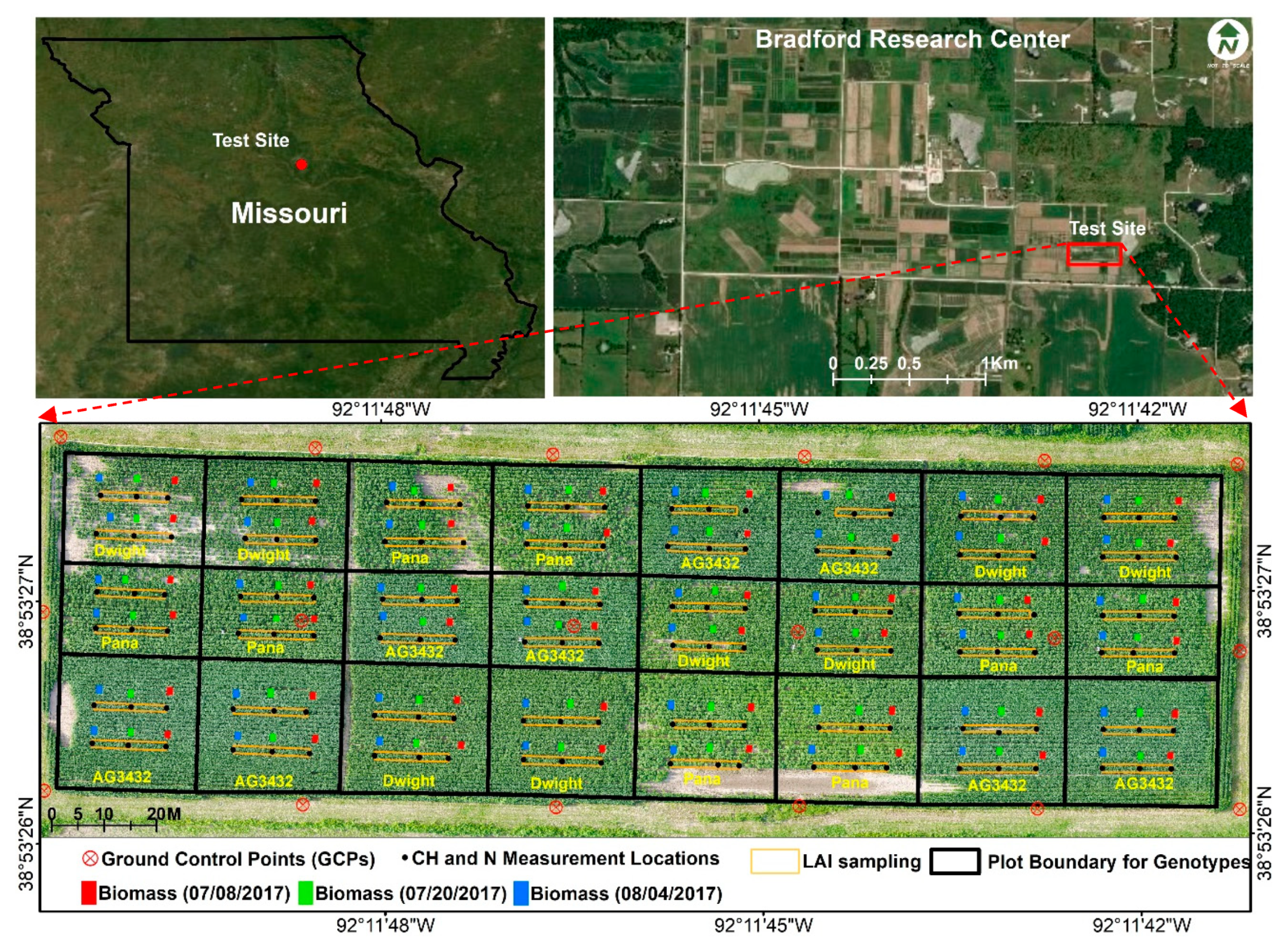
2.1. Test Site and Field Layout

The test site is located at the Bradford Research Center of the University of Missouri in Columbia, Missouri, USA (Figure 1). The average monthly temperature measured by a nearby on-farm weather station was 17.35 °C, 22.63 °C, 25.04 °C, 20.96 °C, 20.16 °C, and 13.75 °C, respectively, from May to October in 2017. The accumulated monthly precipitation was 114 mm, 82 mm, 116 mm, 77 mm, 20 mm, and 98 mm, respectively, from May to October.
As shown in Figure 1, the experiment field was divided into four replications, and each replication was split into rainfed and irrigated main plots, which were planted with three soybean cultivars—‘AG3432’, ‘Pana’, and ‘Dwight’—and sub-plots on May 19th of 2017. A pre- and post-emergence herbicide was applied, along with a manual weed removing to control the weeds. No fertilizers were applied during this experiment.

2.2. Data Acquisition

2.2.1. Field Data Collection

Each AGB sample was harvested from an area of 1 m length and 2 rows width (about 1.52 m2) at locations evenly distributed throughout the field (6 samples within each sub-plot) on 8 July, 20 July, and 4 August, respectively (Figure 1), and oven-dried at 60 °C immediately after harvesting. UAV RGB orthomosaics acquired before and after biomass harvesting were co-reregistered and overlapped to identify the precise sampling locations of AGB [42].
Soybean LAI measurements were carried out at 48 sampling spots throughout the field (two sampling spots within each sub-plot, and each sampling spot was about 21.3 m2 composed of two rows (1.52 m) with about 14 m length) (Figure 1) on 8 July, 20 July, and 4 August, respectively. LAI value was achieved nondestructively using the LAI-2200C Plant Canopy Analyzer (LI-COR Inc., Lincoln, NE, USA) along a diagonal transect between the two rows at each sampling spot. Leaf nitrogen concentration was estimated based on DUALEX 4 Scientific (Force-A, Orsay, France) hand-held device measurements from three leaves at each sampling spot [4], and a total of 144 samples (6 samples within each sub-plot) were collected on 8 July, 20 July, and 4 August, respectively. Field-based canopy height (CH) measurement was conducted using a measuring stick at the same 144 locations where the leaf nitrogen concentration measurements were taken during each sampling day to validate UAV-derived CH. A summary of the field-measured plant trait variables is shown in Table 1.

2.2.2. Remote Sensing Data

UAV-based image acquisition was conducted on the same dates as ground truth plant trait data collection (Table 2). WorldView-2/3 (WV-2/3) (Digital Globe Inc.) imagery was acquired on 10 July 2017, 22 July 2017, and 9 August 2017 as closely as possible to the dates of UAV flights and ground truth data collection. As demonstrated in Table 2, WV-2 data had one panchromatic band and eight visible near-infrared (VNIR) bands. WV-3 data included one panchromatic band, eight VNIR bands, along with eight short wave infrared (SWIR) bands. Due to the coarser resolution of SWIR bands of WV-3, only the VNIR bands were employed for analysis in this study.
UAV RGB imagery was acquired at an altitude of 30 m using a light-weight commercial platform DJI Mavic Pro quadcopter. The flight speed was set to 6 m s−1, and the side and front overlap was 85%. Equipped with a 12.4-Mpixel RGB camera and built-in GPS device, DJI Mavic Pro provides automatically geotagged and high-resolution RGB images [41].

2.3. Image Preprocessing

2.3.1. Worldview Data Preprocessing

Atmospheric correction and radiometric calibration were carried out for WV-2/3 imagery through the Fast Line-of-Sight Atmospheric Analysis of Spectral Hypercubes (FLAASH) method using ENVI 5.4.1 software (Harris Visual Information Solutions, Boulder, CO, USA) [57,58]. Pan-sharpened WV-2/3 imagery with 0.3 m spatial resolution was generated using the Gram–Schmidt Pan Sharpening tool of ENVI 5.4.1 software [23].

2.3.2. UAV Imagery Preprocessing
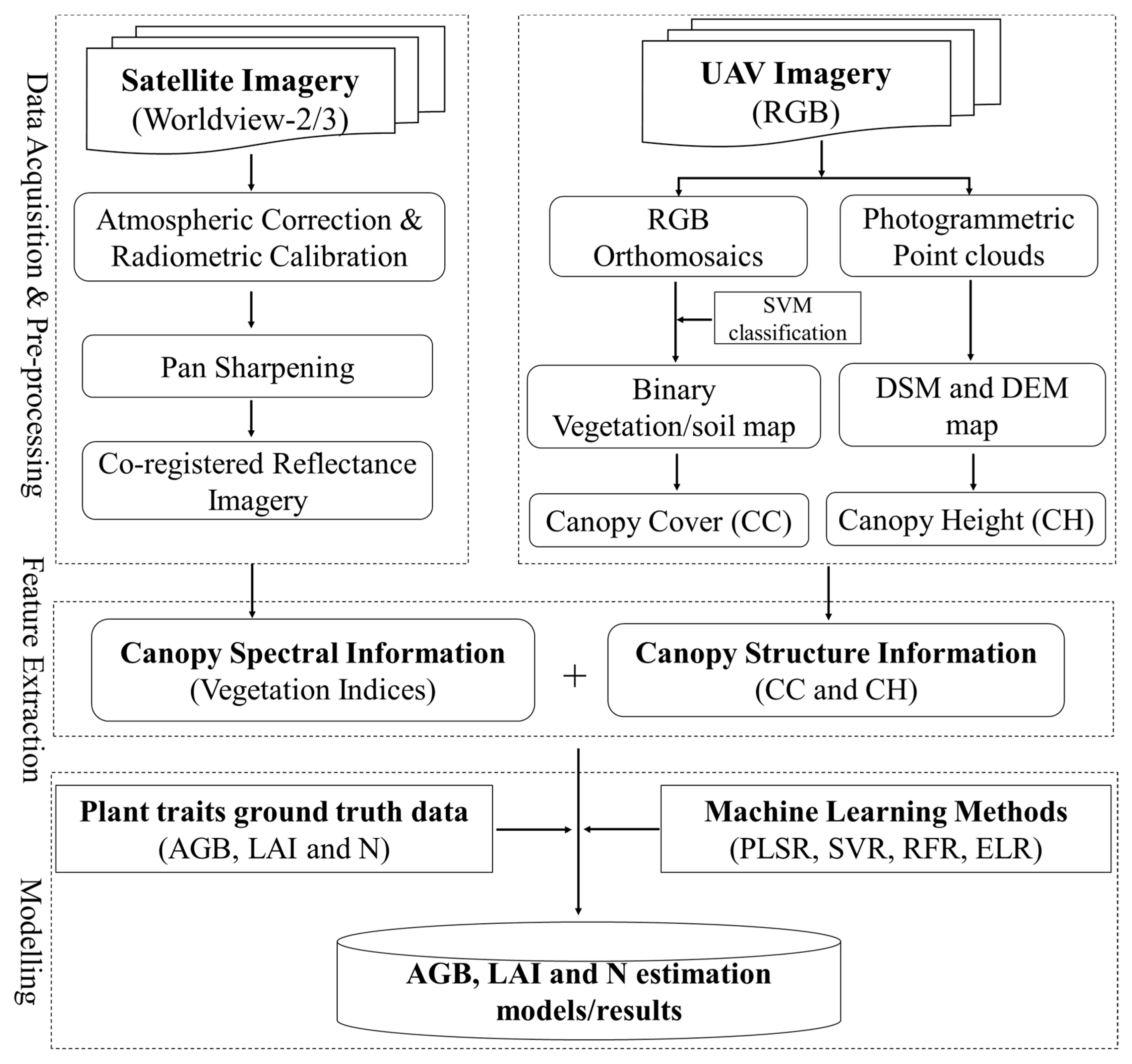
Orthorectification and mosaicking of UAV imagery collections from different sampling days were carried out using Pix4Dmapper software (Pix4D SA, Lausanne, Switzerland). Eighteen highly accurate ground control points (GCPs) (Figure 1) surveyed with a Trimble R8 GNSS Rover (10 mm and 20 mm accuracy at the horizontal and vertical direction, respectively) were leveraged through the processing workflow of Pix4Dmapper, to generate UAV RGB orthomosaics with precise scale and position [42]. Along with the SfM-based photogrammetric workflow embedded in Pix4Dmapper, high density and accurate point clouds were created.
Multitemporal multiscale WV-2/3 imagery and UAV orthomosaics were co-registered and georeferenced to the UAV orthomosaic of July 8, 2017, through a number of GCPs, along with selected ground feature points, such as road intersections, using ArcGIS 10.4 software. The georeferencing errors were less than one pixel (<0.3 m). Finally, a unified and overlapped imagery dataset was generated with WGS 1984 UTM Zone 15N geoinformation.

3. Methods

3.1. Feature Extraction

3.1.1. Satellite Imagery-Based Spectral Feature Extraction

As listed in Table 3, the eight VNIR bands of WV-2/3, as well as a series of VIs employed for crop monitoring in previous research, were selected.

3.1.2. UAV Imagery-Based Canopy Height Extraction

Digital elevation model (DEM) was retrieved using the photogrammetric point clouds from UAV imagery acquired before plant development on 25 May 2017. Additionally, the digital surface model (DSM) for the soybean field was generated on three dates (i.e., 8 July, 20 July, and 4 August 2017) that represent different developmental stages using the UAV imagery-derived point clouds. The subtraction of DEM from DSM was conducted at the pixel level, and the canopy height model (CHM) was created [40].

3.1.3. UAV Imagery-Based Canopy Cover Extraction

The weeds and soil pixels were identified and removed from the UAV RGB orthomosaics from 8 July, 20 July and 4 August, respectively, using the Support Vector Machine (SVM) classifier [74]. An overall accuracy higher than 99% and a Kappa coefficient over 0.99 were achieved from the SVM classifier [42].
Additionally, canopy cover (CC), which reflects the crop density and structure (i.e., LAI) information [75], was computed by dividing the area of soybean canopy pixels in each sampling spot by the total number of pixels within that spot [3]. The formula for CC is as follows:
C C = N u m b e r   o f   soybean   canopy     p i x e l s   i n   t h e   p l o t T o t a l   n u m b e r   o f   p l o t   p i x e l s  
The plot-level average of VIs and CH values were computed in order to relate them to the corresponding AGB, LAI, and N data. Binary masks were applied to remove soil/weed pixels from VIs and CH raster layers. The workflow including image preprocessing, feature extraction, model calibration and validation was demonstrated in Figure 2.

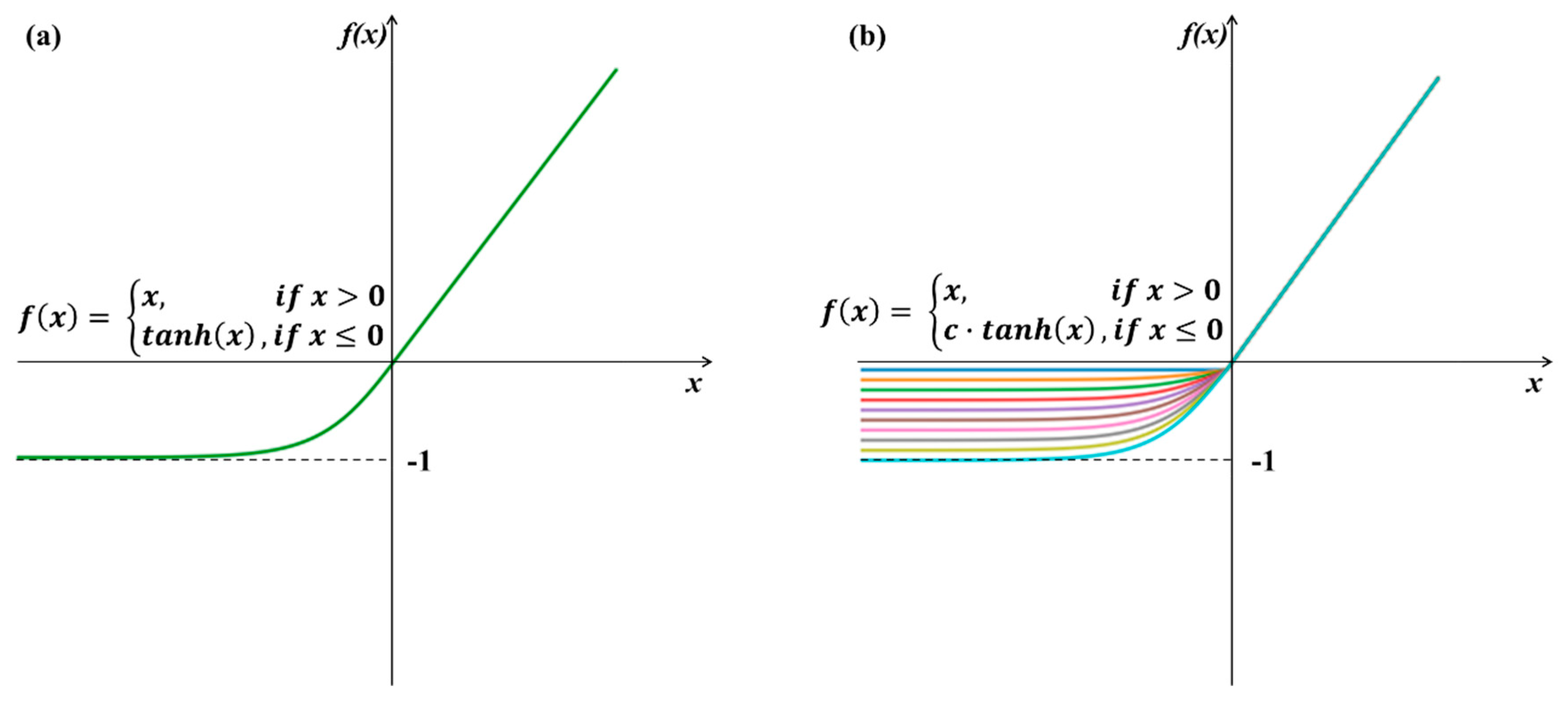
3.2. Modeling Methods
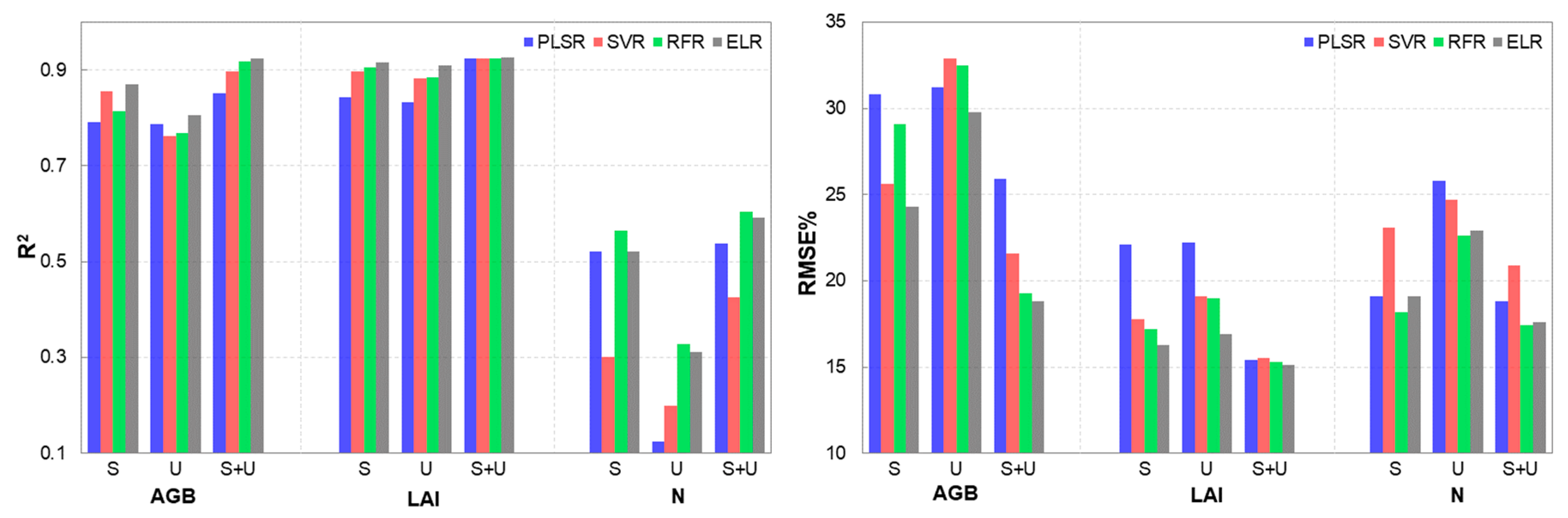
Several commonly used ML methods in remote sensing applications, particularly in crop monitoring and plant traits estimation, such as PLSR, RFR, and SVR [4,40,76], were implemented to estimate AGB, LAI, and N using satellite image-derived VIs and UAV image-based CH and CC (Table 3) as input features. PLSR is a widely-used multivariate statistical technique and is often used to construct predictive models when the number of explanatory variables is large and highly correlated/collinear. It reduces the dimension and noise and transforms the collinear input features to a few non-correlated latent variables by performing component projection [77]. PLSR is similar to principal component regression (PCR), but PLSR uses both the variation of the spectra and the response variable to construct new explanatory components/variables [78]. RFR is a non-parametric ensemble method, which has roots in classification and regression trees (CART); RFR consists of different trees that are trained by applying bagging and random variable selection process [79]. RFR has a better tolerance for outliers and noise [80]. SVR is the implementation of SVM [74] for regression and function approximation. SVR basically converts the nonlinear regression into a linear projection through different kernel functions and transforms the original feature space into a new data space and multidimensional hyperplanes [81]. ELR is the regression version of ELM; the classic ELM is a feedforward neural network, which has one input layer, one hidden layer, and one output layer. Instead of iterative tuning, the hidden node parameters in ELM are randomly generated, which provides high computational efficiency [51].
In this study, a dual activation function-based extreme learning machine (ELM), which has been proved to outperform regular ELM for crop monitoring application in previous research [82], was modified and implemented. In our previous study [82], the activation function, namely, TanhRe, that combines rectified linear unit (ReLU) [83] and hyperbolic tangent (Tanh) functions have shown superior performance for grapevine yield and berry quality prediction, compared to commonly used nonlinear functions, such as sigmoid, Tanh, and ReLU (Figure 3a). Inspired by leaky ReLU, we herein proposed a modified TanhRe by introducing a small coefficient to Tanh function, instead of using the fixed shape of Tanh, which allowed for a flexible functionality to better fit the input pattern. Accordingly, the proposed activation function was defined as:
f ( x ) = { x , i f   x > 0 c · tanh ( x ) ,     i f   x 0
where x is the input of the nonlinear activation f , and c is a small constant, such as 0.001. In this paper, the constant c was optimized using the value from 0 to 1 (Figure 3b).
For implementing different ML methods, 70% of input features were randomly selected and used together with corresponding AGB, LAI, and N data for model training, and the remaining 30% unseen data were used to test the model. All variables, including VIs, CH, and CC, were used as input features for the modeling, and no feature selection method was applied. A grid-search and k-fold cross-validation technique were applied to obtain optimal parameters for each method during the model calibration phase [84]. For the PLSR method, the number of principal components (PCs) was determined by the grid search. A radial basis kernel function (RBF) was used for SVR, and the kernel parameter gamma and regularization parameter C were determined by tuning. The number of trees for the RFR method was set at 500, and the max_features parameter, which decides how many features each tree in the RFR considers at each split, was determined through the grid search procedure. For the ELR method, the number of neurons in the hidden layer, the generalization parameter C, as well as the proposed activation function’s coefficient c, were optimized through the grid search. The assessment of model performance was conducted by adopting the root mean square error (RMSE), relative RMSE (RMSE%), along with the coefficients of determination (R2). The equations were as follows:
RMSE = i = 1 n ( y i y ^ i ) 2 n 1
RMSE %   = RMSE y ¯ 100
where y ^ i and yi represent the predicted and the measured AGB, LAI, and N data, respectively. y ¯ is the average of each measured variable, and n is the sample size used for model testing.

4. Results

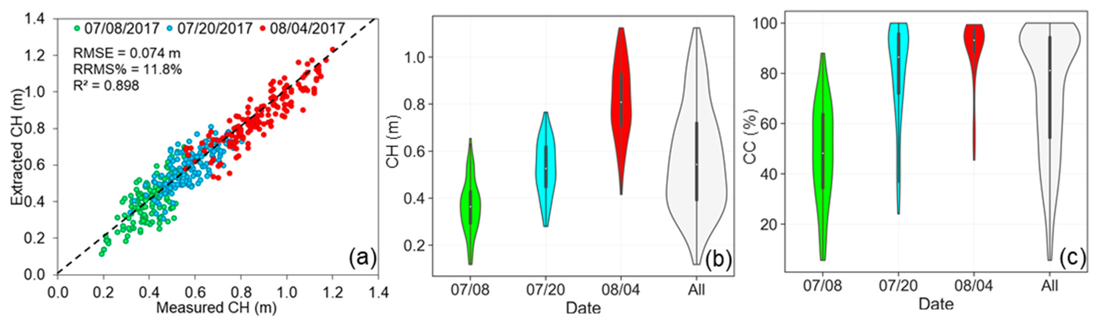
4.1. Distribution of Canopy Height and Canopy Cover

UAV imagery-derived CH was validated by comparing to the manual measurements made in the field (Figure 4a), which presented R2 of 0.898 and RMSE% of 11.8%. As documented in past studies [42,85], photogrammetric point cloud-based CH of smaller plants (i.e., 0.3 m in this case) were slightly underestimated, which might be due to missing points during the point cloud reconstruction and post-processing [86]. The distribution of UAV imagery-derived CH at different developmental stages and across all stages was displayed with violin plots (Figure 4b). CH ranged considerably within each developmental stage, especially on July 20 and August 4, which indicated a large spatial variability and heterogeneity of canopy structure in the vertical direction of soybean. This was likely due to a number of factors, including variation associated with soybean genotypes, soil conditions, and water availability. UAV imagery-extracted CC also demonstrated relatively wide data ranges (Figure 4c), especially at the early development stage (i.e., 08 July), which also implied spatial variety and heterogeneity of soybean canopy. However, due to the gradual closing of the soybean canopy from July 8 to August 4, the variation in CC became smaller, and the CC of the most area approached 100% (Figure 4c).

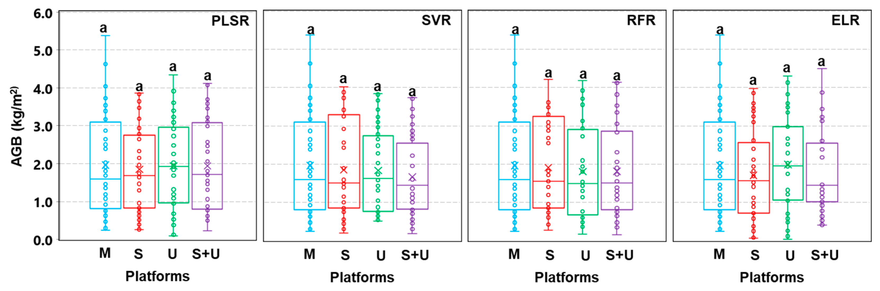
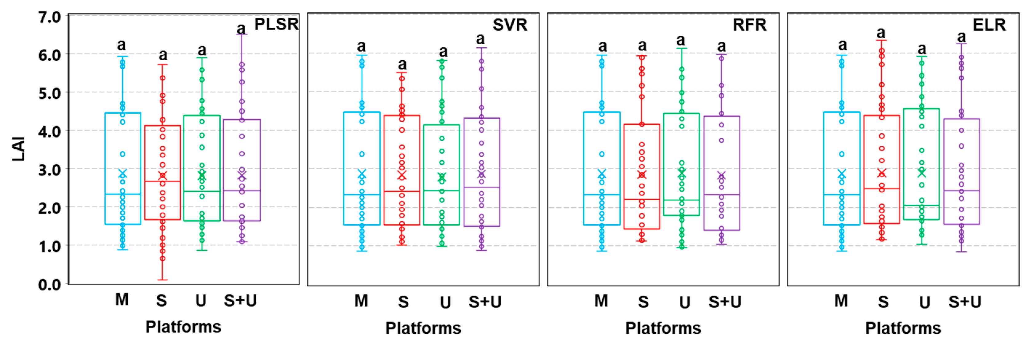
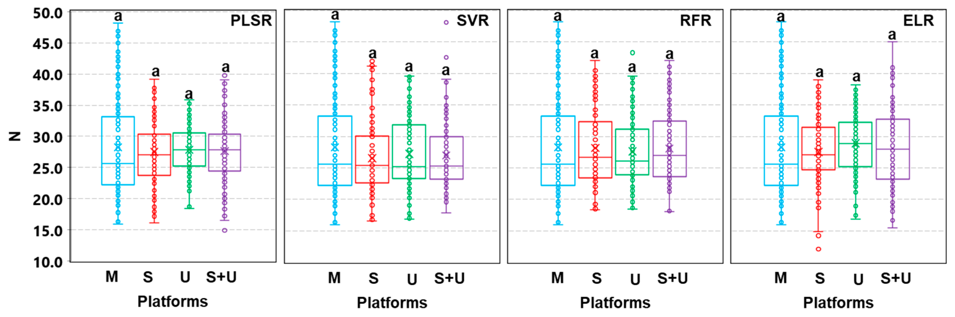
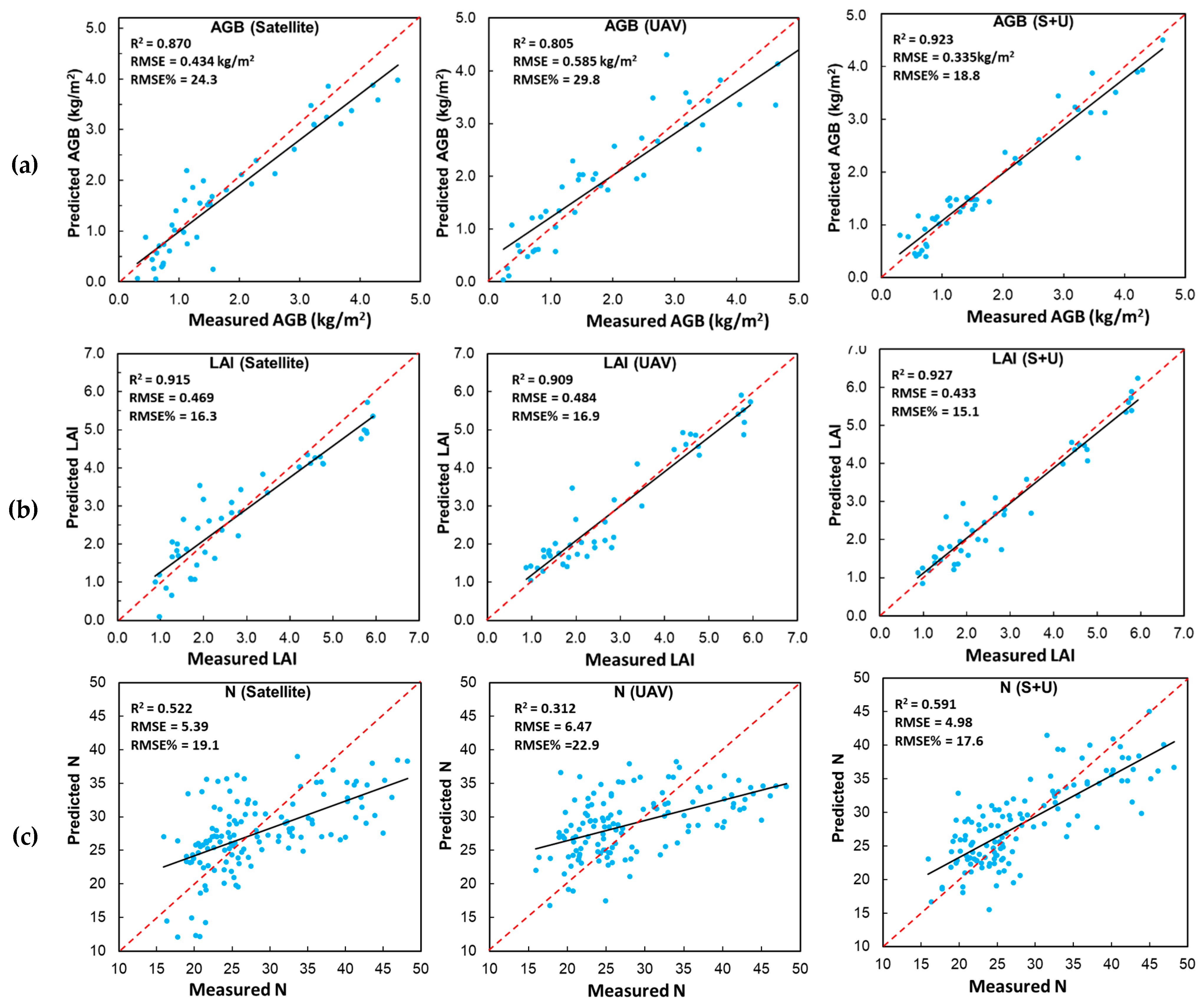
4.2. Estimation Results of AGB, LAI, and N

PLSR, SVR, RFR, and ELR were employed for AGB, LAI, and N prediction using satellite-based canopy spectral information, UAV-based canopy structure information, as well as the combination of spectral and structure information, respectively.
The validation metrics for AGB estimation are demonstrated in Table 4. Satellite-based spectral information yielded superior performance to UAV-based canopy structure information (i.e., CH and CC) regardless of regression models with R2 ranging from 0.792 to 0.870 and RMSE% from 30.8% to 24.3%. Structure information presented lesser, yet comparable performance with R2 from 0.763 to 0.805 and RMSE% from 32.9% to 29.8%. A combination of satellite/UAV spectral and structure information produced the best results with R2 varying from 0.852 to 0.923 and RMSE% from 25.9% to 18.8%.
Additionally, the predicted AGB values using satellite, UAV, and their combination, as well as measured AGB values, were compared using ANOVA with HSD Tukey tests (α = 0.05). The results showed that no significant differences were found between predicted AGB when using data from different platforms (Figure 5), as well as between measured and predicted AGB, demonstrating that data from different platforms was effective in predicting AGB regardless of the regression methods.
As shown in Table 5, satellite imagery-derived canopy spectral information slightly outperformed UAV-based canopy structure information for LAI estimation with R2 varying from 0.844 to 0.915 and RMSE% from 22.1% to 16.3%. UAV-derived canopy structure information provided decent and comparable results to satellite spectral information with R2 ranging from 0.832 to 0.909 and RMSE% from 22.2% to 16.9%. The integration of spectral information with structure features boosted the prediction accuracy with R2 varying from 0.923 to 0.927 and RMSE% from 15.5% to 15.1%.
In addition, the measured LAI, as well as the predicted LAI values, using data from satellite, UAV, and their combination were compared using ANOVA with HSD Tukey tests (α = 0.05). The results showed that no significant differences were found between measured and predicted LAI, as well as among predicted LAI using different platforms’ data regardless of the regression methods (Figure 6). This indicated that data from different platforms was effective in predicting LAI regardless of the regression methods.
Validation statistics of leaf N estimation are displayed in Table 6. Overall, whether based on satellite or UAV individually, as well as in combination, the estimation of leaf N was poor. However, satellite-based canopy spectral information yielded superior performance to UAV-based canopy structure information with R2 ranging from 0.301 to 0.565 and RMSE% from 23.1% to 18.2%. UAV-derived canopy structure features presented poorer performance with R2 varying from 0.125 to 0.328 and RMSE% from 25.8% to 22.6%. Although at a minor scale, the inclusion of canopy structure information with spectral features improved the estimation accuracy of N regardless of the regression models.
The estimated N values using data from satellite, UAV, and their combination were compared with each other and also against measured N using ANOVA with HSD Tukey tests (α = 0.05). The results showed that no significant differences were found between measured and predicted N, as well as among predicted N using different platforms’ data regardless of the regression methods (Figure 7). This indicated that data from different platforms was effective in predicting N regardless of the regression methods.

5. Discussion

5.1. Satellite/UAV Data Fusion and Its Impact on Model Performance

Canopy spectral features (i.e., VIs) have been extensively used in the realm of remote sensing-based crop monitoring and agricultural applications. As shown in Table 4, Table 5 and Table 6, regardless of the regression models, canopy spectral information outperformed structure features for AGB, LAI, and N estimation, which agreed with previous studies [4,87]. In detail, canopy structure features yielded slightly lesser, yet comparable performance to spectral features for AGB and LAI prediction. This indicated, to some extent, that canopy structure features are promising alternatives to spectral VIs for remote sensing-based crop monitoring. Many previous studies have noted the potential of canopy structure features in the estimation of AGB [42,88], LAI [4], and leaf N [89]. Due to the complementary information provided by satellite-based abundant spectral features and UAV-derived structure features, satellite/UAV data fusion boosted the model performance compared with the satellite or UAV data alone (Table 4, Table 5 and Table 6). Canopy structure features (i.e., CH and CC) contain independent information on canopy growth and architecture [12,90], which is supplementary for spectral information to some extent, and eventually improve model performance [4,91,92,93].
Compared with the estimation of AGB and LAI, canopy structure features have been rarely used for N estimation in remote sensing applications. In our case, canopy structure features produced a poor performance for N estimation; however, integrating canopy structure features with spectral features was able to improve model performance regardless of the regression methods (Table 6). It is worth noting that both improved model performance [94,95,96], as well as no improvement [89], have been documented for N estimation when the inclusion of canopy structure features to VIs in previous studies. Additionally, the hand-held sensor used for N estimation measured a small area (19.6 mm2) of a single leaf per measurement, and, even when 6 measurements were taken per plot, some error was expected to be associated with respect to the representativeness of these spot measurements for the canopy. Further research efforts are needed to investigate the potential of canopy structure features for the estimation of leaf biochemical traits, such as leaf N concentration over different environments and crop species. Additionally, the application of alternative ground-truth measurements should be investigated to improve the predictions of biochemical traits.

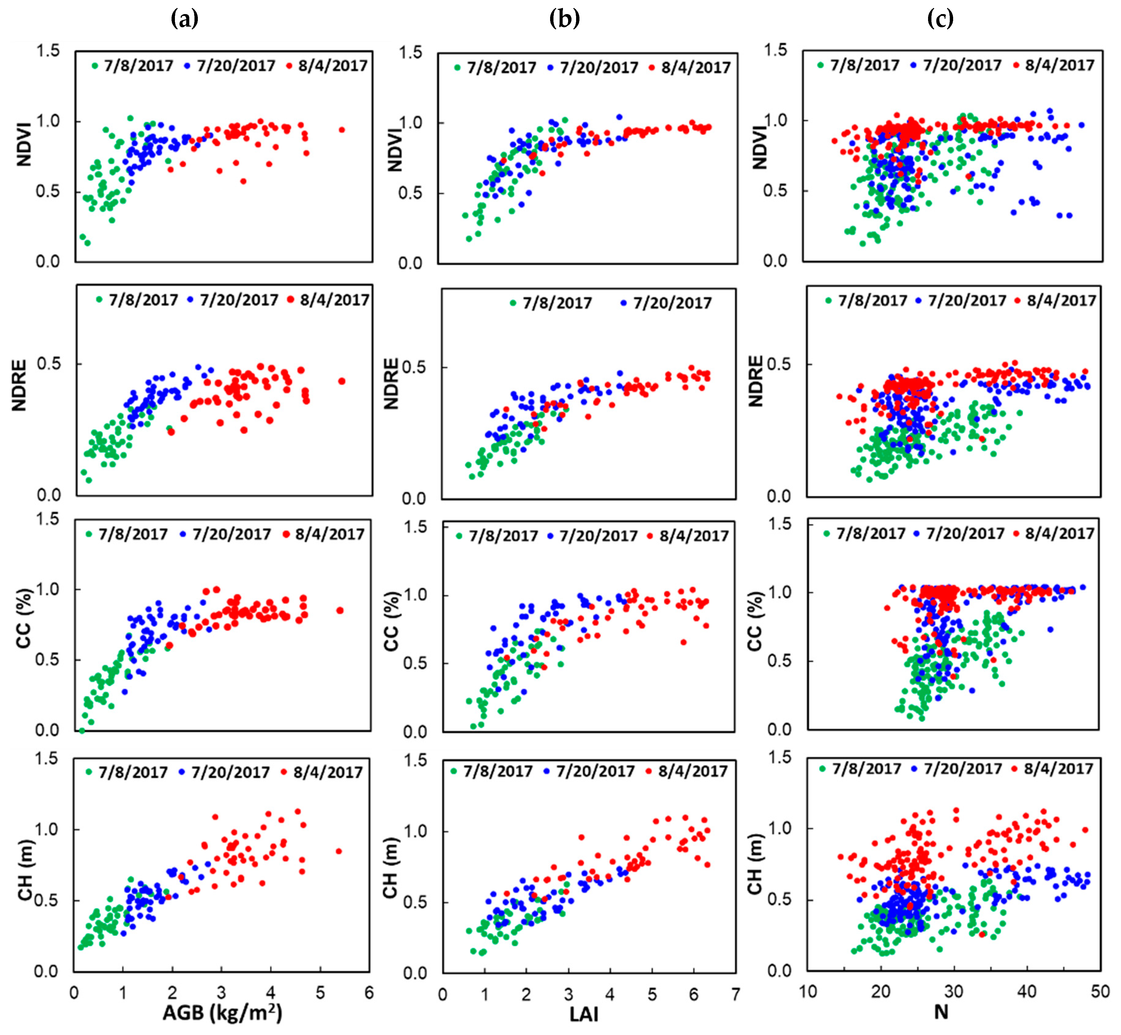
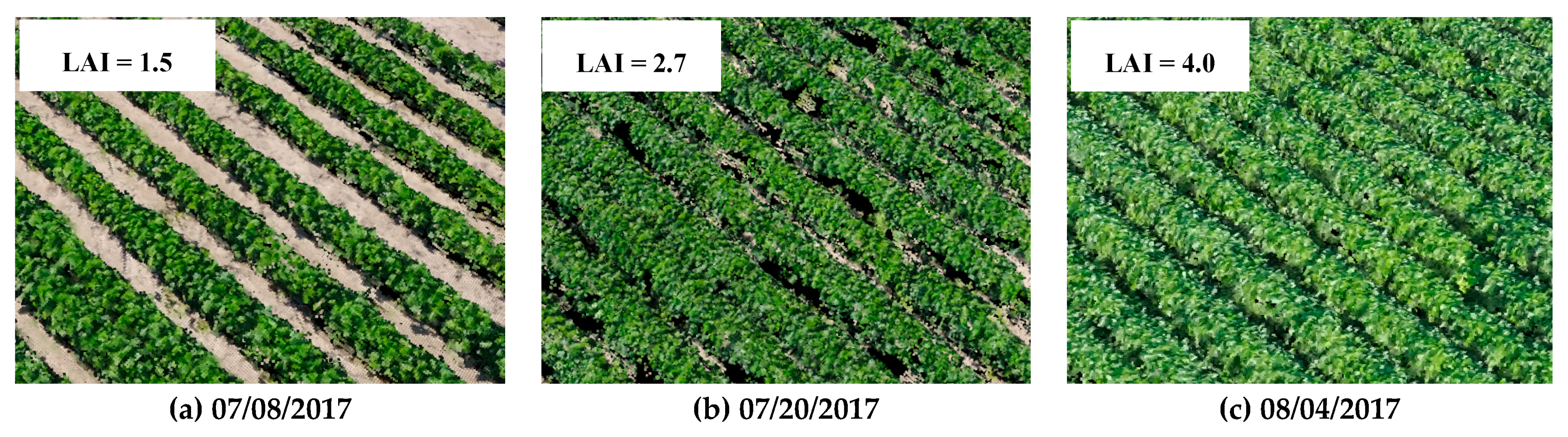
5.2. Canopy Structure Information and Spectral Saturation Issue

The asymptotic saturation phenomenon has been widely recognized as an issue for optical remote sensing-based crop monitoring (i.e., crop AGB, LAI, and N estimation). It characterizes one of the major limitations of optical remote sensing data, especially using such data collected from dense and heterogeneous canopies [11,12,40]. Canopy spectral features represented by commonly used VIs, such as Normalized Difference Vegetation Index (NDVI) and Normalized Difference Red Edge (NDRE), along with canopy structure features CH and CC, were plotted against AGB, LAI, and N (Figure 8). With the increase of AGB, LAI, and N (Figure 8) at the late developmental stage (i.e., August 4, represented by red dots in Figure 8), both NDVI and NDRE increased only slightly or did not increase accordingly, presenting gradual saturation patterns. Additionally, canopy structure feature CC also displayed the saturation pattern. Asymptotic saturation of canopy spectral features is a challenge for estimating plant traits of crops planted at high density and leads to lower accuracy [26]. However, CH demonstrated higher responsiveness to the increase of AGB, LAI, and N, which led to the weakening of saturation issue, and eventually improved the model accuracy to some extent [4].
Due to the superior performance of ELR compared to other models, estimates of AGB, LAI, and N achieved from ELR were plotted against their corresponding ground truth values (Figure 9). AGB, LAI, and N were underestimated for samples with higher values, particularly in the case of using spectral data alone, which is likely attributed to the saturation issue [97,98]. Consistent with the previous study by Moeckel, Safari, Reddersen, Fricke and Wachendorf [8], obvious improvement of fit was observed for all variables when combining canopy spectral and structure features. This was demonstrated by higher R2 and lower RMSE%, as well as the convergence of the linear fitting line (black solid line in Figure 9) and the bisector (red dash line), implying that the saturation effect was reduced to some extent when employing satellite/UAV data fusion for crop monitoring.

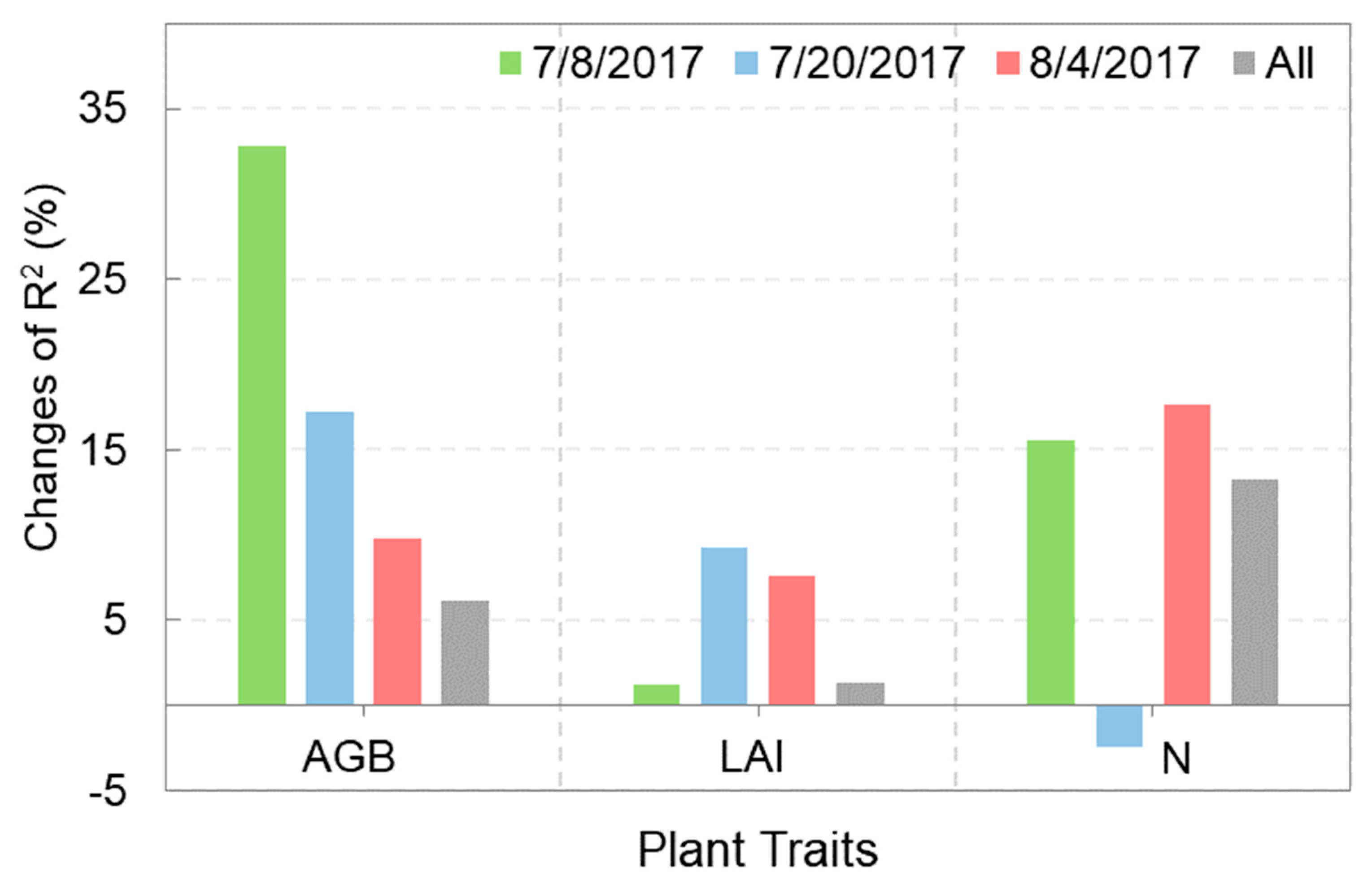
5.3. Contribution of Data Fusion at Different Crop Developmental Stages

ELR with the newly proposed activation function stably yielded the best performance for AGB, LAI, and N prediction compared to other ML methods in most of the cases (Table 4, Table 5 and Table 6). Thus, it was employed for generating prediction results at different development stages of soybean (Table 7).
Overall, the inclusion of UAV-derived canopy structure information to satellite-based spectral features improved the model performance of AGB, LAI, and N estimation at all developmental stages, except for N estimation on July 20 (Table 7 and Figure 10). Canopy structure features (i.e., CH and CC) provide independent information on canopy growth and architecture [12,90] and supplement canopy spectral features in terms of AGB, LAI, and N estimation [4,91,92,93], which likely contributes to improved model performance. Additionally, as evidenced in Figure 11, background soil reflectance, especially at early stages (i.e., July 8) [99,100,101], as well as saturation issue due to dense/closed canopy (Figure 11c) at a late stage (i.e., 4 August) [35,102], affected the performance of satellite data-based crop monitoring. Thus, the improvement of model performance when adding high-resolution canopy structure features to VIs indicated that canopy structure features likely weakened the effects of soil background and saturation issues.
It is worth noting that satellite/UAV data fusion was not able to improve the model performance of leaf N estimation on July 20. The unstable performance of CH at different developmental stages, when combined with spectral data in N estimation, has also been reported previously by Näsi, Viljanen, Kaivosoja, Alhonoja, Hakala, Markelin and Honkavaara [89]. This might be due to the inferior correlation between UAV-derived features and leaf N on July 20 compared with the other developmental stages (Table 7), as well as possible information homogeneity and redundancy between canopy spectral and structure features [103]. Further investigation should be conducted to examine the potential/possibility of canopy structure features for leaf N estimation at different development stages over different crop species and environments. In addition, alternative methods of ground-truthing N concentration should be examined to improve the predictions of biochemical traits.

5.4. Comparison of Different Modeling Methods

As evidenced by high R2 and low RMSE% (Figure 12), ELR produced the most accurate model in AGB and LAI estimation, which matched results obtained in previous studies [4,104]. This could be attributed to the nonlinear learning capability of integrated ReLU and tanh activation functions, along with the insensitivity to outliers of the adjusted ELR model [82]. Additionally, the newly introduced coefficient (Figure 3b and Equation (2)) to ELR’s dual activation function in this study possessed more robust and flexible functionality to better capture the input feature patterns and eventually led to the improvement of model performance. For N estimation, RFR yielded the best performance with the highest R2 and lowest RMSE% (Figure 12). RFR shows higher tolerance for data faults with a large sample decision tree for high dimensional data training [79]. SVR provided decent accuracies, which were comparable to RFR in most cases in this study. SVR also can cope with high data dimensionality but is less sensitive to sample size compared to RFR [105]. It is worth noting that RFR and SVR are the most extended ML algorithms in remote sensing-based crop monitoring applications, and their potential in handling nonlinear and noisy data, as well as dealing with overfitting issues, is well documented [106,107,108]. The PLSR model was outperformed by other models in most of the cases as it resulted in lower R2 and higher RMSE% (Figure 12). PLSR technique is able to tackle multiple collinearity problems through principal component analysis; however, its limitation, particularly in dealing with non-linear and complex relationships between plant traits and spectral features, has been noted in the literature [107].

6. Conclusions

The main merit of this research was the demonstration of a novel application for crop monitoring across a heterogeneous soybean field in the framework of satellite/UAV data fusion and machine learning. The main conclusions were:
1. With the capability of providing high-resolution and detailed 3-dimensional canopy structure information (i.e., canopy height and canopy cover), low-cost UAV integrated with RGB camera was a promising tool to supplement satellite-based crop monitoring.
2. UAV-derived high-resolution and detailed canopy structure features (i.e., canopy height and canopy cover) were significant indicators for crop monitoring. Combing satellite imagery-based rich canopy spectral information with UAV-derived canopy structural features using machine learning was able to improve crop AGB, LAI, leaf N concentration estimation. Additionally, the inclusion of canopy structure information to spectral features tended to reduce background soil effect and asymptotic saturation issues.
3. The ELR model with the proposed activation function slightly outperformed PLSR, RFR, and SVR methods in the prediction of AGB and LAI, while RFR yielded the best performance for leaf N concentration estimation.
The results of this study illustrated the tremendous potential of satellite/UAV synergy in the context of crop monitoring using machine learning. Nevertheless, the approach employed in this study should be tested across different field environments, as well as a variety of crop types.

Author Contributions

Conceptualization, M.M., V.S., and P.S.; methodology, M.M. and P.S.; software, M.M. and P.S.; validation, M.M., V.S., P.S., and F.B.F.; investigation, M.M., P.S., A.M.D., and H.E.; resources, V.S. and F.B.F.; writing—original draft preparation, M.M; writing—review and editing, M.M., V.S., P.S., and F.B.F.; supervision, V.S.; project administration, V.S.; funding acquisition, V.S. All authors have read and agreed to the published version of the manuscript.

Funding

This research was funded in part by the National Science Foundation (IIA-1355406 and IIA-1430427), and in part by the National Aeronautics and Space Administration (NNX15AK03H).

Acknowledgments

The authors thank the UAV data collection team from the Remote Sensing Lab at Saint Louis University and the assistance of the Crop Physiology Lab at the University of Missouri in Columbia in the field management and data collection.

Conflicts of Interest

The authors declare no conflict of interest.

References

  1. Schut, A.G.; Traore, P.C.S.; Blaes, X.; Rolf, A. Assessing yield and fertilizer response in heterogeneous smallholder fields with UAVs and satellites. Field Crop. Res. 2018, 221, 98–107. [Google Scholar] [CrossRef]
  2. Araus, J.L.; Cairns, J.E. Field high-throughput phenotyping: The new crop breeding frontier. Trends Plant Sci. 2014, 19, 52–61. [Google Scholar] [CrossRef]
  3. Yu, N.; Li, L.; Schmitz, N.; Tian, L.F.; Greenberg, J.A.; Diers, B.W. Development of methods to improve soybean yield estimation and predict plant maturity with an unmanned aerial vehicle based platform. Remote Sens. Environ. 2016, 187, 91–101. [Google Scholar] [CrossRef]
  4. Maimaitijiang, M.; Ghulam, A.; Sidike, P.; Hartling, S.; Maimaitiyiming, M.; Peterson, K.; Shavers, E.; Fishman, J.; Peterson, J.; Kadam, S. Unmanned Aerial System (UAS)-based phenotyping of soybean using multi-sensor data fusion and extreme learning machine. ISPRS J. Photogramm. Remote Sens. 2017, 134, 43–58. [Google Scholar] [CrossRef]
  5. Marshall, M.; Thenkabail, P. Advantage of hyperspectral EO-1 Hyperion over multispectral IKONOS, GeoEye-1, WorldView-2, Landsat ETM plus, and MODIS vegetation indices in crop biomass estimation. ISPRS J. Photogramm. Remote Sens. 2015, 108, 205–218. [Google Scholar] [CrossRef] [Green Version]
  6. Liu, J.G.; Pattey, E.; Jego, G. Assessment of vegetation indices for regional crop green LAI estimation from Landsat images over multiple growing seasons. Remote Sens. Environ. 2012, 123, 347–358. [Google Scholar] [CrossRef]
  7. Sagan, V.; Maimaitijiang, M.; Sidike, P.; Eblimit, K.; Peterson, K.T.; Hartling, S.; Esposito, F.; Khanal, K.; Newcomb, M.; Pauli, D. Uav-based high resolution thermal imaging for vegetation monitoring, and plant phenotyping using ici 8640 p, flir vue pro r 640, and thermomap cameras. Remote Sens. 2019, 11, 330. [Google Scholar] [CrossRef] [Green Version]
  8. Moeckel, T.; Safari, H.; Reddersen, B.; Fricke, T.; Wachendorf, M. Fusion of ultrasonic and spectral sensor data for improving the estimation of biomass in grasslands with heterogeneous sward structure. Remote Sens. 2017, 9, 98. [Google Scholar] [CrossRef] [Green Version]
  9. Jackson, R.D.; Huete, A.R. Interpreting vegetation indices. Prev. Vet. Med. 1991, 11, 185–200. [Google Scholar] [CrossRef]
  10. Wang, C.; Nie, S.; Xi, X.H.; Luo, S.Z.; Sun, X.F. Estimating the Biomass of Maize with Hyperspectral and LiDAR Data. Remote Sens. 2017, 9, 11. [Google Scholar] [CrossRef] [Green Version]
  11. Greaves, H.E.; Vierling, L.A.; Eitel, J.U.H.; Boelman, N.T.; Magney, T.S.; Prager, C.M.; Griffin, K.L. Estimating aboveground biomass and leaf area of low-stature Arctic shrubs with terrestrial LiDAR. Remote Sens. Environ. 2015, 164, 26–35. [Google Scholar] [CrossRef]
  12. Rischbeck, P.; Elsayed, S.; Mistele, B.; Barmeier, G.; Heil, K.; Schmidhalter, U. Data fusion of spectral, thermal and canopy height parameters for improved yield prediction of drought stressed spring barley. Eur. J. Agron. 2016, 78, 44–59. [Google Scholar] [CrossRef]
  13. Puliti, S.; Saarela, S.; Gobakken, T.; Ståhl, G.; Næsset, E. Combining UAV and Sentinel-2 auxiliary data for forest growing stock volume estimation through hierarchical model-based inference. Remote Sens. Environ. 2018, 204, 485–497. [Google Scholar] [CrossRef]
  14. Mutanga, O.; Skidmore, A.K. Narrow band vegetation indices overcome the saturation problem in biomass estimation. Int. J. Remote Sens. 2004, 25, 3999–4014. [Google Scholar] [CrossRef]
  15. Delegido, J.; Verrelst, J.; Meza, C.; Rivera, J.; Alonso, L.; Moreno, J. A red-edge spectral index for remote sensing estimation of green LAI over agroecosystems. Eur. J. Agron. 2013, 46, 42–52. [Google Scholar] [CrossRef]
  16. Haboudane, D.; Miller, J.R.; Pattey, E.; Zarco-Tejada, P.J.; Strachan, I.B. Hyperspectral vegetation indices and novel algorithms for predicting green LAI of crop canopies: Modeling and validation in the context of precision agriculture. Remote Sens. Environ. 2004, 90, 337–352. [Google Scholar] [CrossRef]
  17. Delegido, J.; Verrelst, J.; Alonso, L.; Moreno, J. Evaluation of sentinel-2 red-edge bands for empirical estimation of green LAI and chlorophyll content. Sensors 2011, 11, 7063–7081. [Google Scholar] [CrossRef] [Green Version]
  18. Clevers, J.G.; Gitelson, A.A. Remote estimation of crop and grass chlorophyll and nitrogen content using red-edge bands on Sentinel-2 and-3. Int. J. Appl. Earth Obs. Geoinf. 2013, 23, 344–351. [Google Scholar] [CrossRef]
  19. Wang, W.; Yao, X.; Yao, X.; Tian, Y.; Liu, X.; Ni, J.; Cao, W.; Zhu, Y. Estimating leaf nitrogen concentration with three-band vegetation indices in rice and wheat. Field Crops Res. 2012, 129, 90–98. [Google Scholar] [CrossRef]
  20. Vaglio Laurin, G.; Pirotti, F.; Callegari, M.; Chen, Q.; Cuozzo, G.; Lingua, E.; Notarnicola, C.; Papale, D. Potential of ALOS2 and NDVI to estimate forest above-ground biomass, and comparison with lidar-derived estimates. Remote Sens. 2017, 9, 18. [Google Scholar] [CrossRef] [Green Version]
  21. Schmidt, M.; Carter, J.; Stone, G.; O’Reagain, P. Integration of optical and X-band radar data for pasture biomass estimation in an open savannah woodland. Remote Sens. 2016, 8, 989. [Google Scholar] [CrossRef] [Green Version]
  22. Dalponte, M.; Ørka, H.O.; Ene, L.T.; Gobakken, T.; Næsset, E. Tree crown delineation and tree species classification in boreal forests using hyperspectral and ALS data. Remote Sens. Environ. 2014, 140, 306–317. [Google Scholar] [CrossRef]
  23. Hartling, S.; Sagan, V.; Sidike, P.; Maimaitijiang, M.; Carron, J. Urban Tree Species Classification Using a WorldView-2/3 and LiDAR Data Fusion Approach and Deep Learning. Sensors 2019, 19, 1284. [Google Scholar] [CrossRef] [PubMed] [Green Version]
  24. Blázquez-Casado, Á.; Calama, R.; Valbuena, M.; Vergarechea, M.; Rodríguez, F. Combining low-density LiDAR and satellite images to discriminate species in mixed Mediterranean forest. Ann. For. Sci. 2019, 76, 57. [Google Scholar] [CrossRef]
  25. Badreldin, N.; Sanchez-Azofeifa, A. Estimating forest biomass dynamics by integrating multi-temporal Landsat satellite images with ground and airborne LiDAR data in the Coal Valley Mine, Alberta, Canada. Remote Sens. 2015, 7, 2832–2849. [Google Scholar] [CrossRef] [Green Version]
  26. Cao, L.; Pan, J.; Li, R.; Li, J.; Li, Z. Integrating airborne LiDAR and optical data to estimate forest aboveground biomass in arid and semi-arid regions of China. Remote Sens. 2018, 10, 532. [Google Scholar] [CrossRef] [Green Version]
  27. Zhang, L.; Shao, Z.; Liu, J.; Cheng, Q. Deep Learning Based Retrieval of Forest Aboveground Biomass from Combined LiDAR and Landsat 8 Data. Remote Sens. 2019, 11, 1459. [Google Scholar] [CrossRef] [Green Version]
  28. Pope, G.; Treitz, P. Leaf area index (LAI) estimation in boreal mixedwood forest of Ontario, Canada using light detection and ranging (LiDAR) and WorldView-2 imagery. Remote Sens. 2013, 5, 5040–5063. [Google Scholar] [CrossRef] [Green Version]
  29. Rutledge, A.M.; Popescu, S.C. Using LiDAR in determining forest canopy parameters. In Proceedings of the ASPRS 2006 Annual Conference, Reno, NV, USA, 1–5 May 2006. [Google Scholar]
  30. Jensen, J.L.; Humes, K.S.; Vierling, L.A.; Hudak, A.T. Discrete return lidar-based prediction of leaf area index in two conifer forests. Remote Sens. Environ. 2008, 112, 3947–3957. [Google Scholar] [CrossRef] [Green Version]
  31. Thomas, V.; Treitz, P.; Mccaughey, J.; Noland, T.; Rich, L. Canopy chlorophyll concentration estimation using hyperspectral and lidar data for a boreal mixedwood forest in northern Ontario, Canada. Int. J. Remote Sens. 2008, 29, 1029–1052. [Google Scholar] [CrossRef]
  32. Tonolli, S.; Dalponte, M.; Neteler, M.; Rodeghiero, M.; Vescovo, L.; Gianelle, D. Fusion of airborne LiDAR and satellite multispectral data for the estimation of timber volume in the Southern Alps. Remote Sens. Environ. 2011, 115, 2486–2498. [Google Scholar] [CrossRef]
  33. Dash, J.P.; Watt, M.S.; Bhandari, S.; Watt, P. Characterising forest structure using combinations of airborne laser scanning data, RapidEye satellite imagery and environmental variables. Forestry 2015, 89, 159–169. [Google Scholar] [CrossRef] [Green Version]
  34. Hütt, C.; Schiedung, H.; Tilly, N.; Bareth, G. Fusion of high resolution remote sensing images and terrestrial laser scanning for improved biomass estimation of maize. Int. Arch. Photogramm. Remote Sens. Spat. Inf. Sci. 2014, XL-7, 101–108. [Google Scholar]
  35. Li, W.; Niu, Z.; Wang, C.; Huang, W.; Chen, H.; Gao, S.; Li, D.; Muhammad, S. Combined use of airborne LiDAR and satellite GF-1 data to estimate leaf area index, height, and aboveground biomass of maize during peak growing season. IEEE J. Sel. Top. Appl. Earth Obs. Remote Sens. 2015, 8, 4489–4501. [Google Scholar] [CrossRef]
  36. Höfle, B. Radiometric correction of terrestrial LiDAR point cloud data for individual maize plant detection. IEEE Geosci. Remote Sens. Lett. 2013, 11, 94–98. [Google Scholar] [CrossRef]
  37. Dandois, J.P.; Ellis, E.C. High spatial resolution three-dimensional mapping of vegetation spectral dynamics using computer vision. Remote Sens. Environ. 2013, 136, 259–276. [Google Scholar] [CrossRef] [Green Version]
  38. Walter, J.; Edwards, J.; McDonald, G.; Kuchel, H. Photogrammetry for the estimation of wheat biomass and harvest index. Field Crops Res. 2018, 216, 165–174. [Google Scholar] [CrossRef]
  39. Sankaran, S.; Khot, L.R.; Espinoza, C.Z.; Jarolmasjed, S.; Sathuvalli, V.R.; Vandemark, G.J.; Miklas, P.N.; Carter, A.H.; Pumphrey, M.O.; Knowles, N.R. Low-altitude, high-resolution aerial imaging systems for row and field crop phenotyping: A review. Eur. J. Agron. 2015, 70, 112–123. [Google Scholar] [CrossRef]
  40. Maimaitijiang, M.; Sagan, V.; Sidike, P.; Hartling, S.; Esposito, F.; Fritschi, F.B. Soybean yield prediction from UAV using multimodal data fusion and deep learning. Remote Sens. Environ. 2020, 237, 111599. [Google Scholar] [CrossRef]
  41. Sidike, P.; Sagan, V.; Qumsiyeh, M.; Maimaitijiang, M.; Essa, A.; Asari, V. Adaptive trigonometric transformation function with image contrast and color enhancement: Application to unmanned aerial system imagery. IEEE Geosci. Remote Sens. Lett. 2018, 15, 404–408. [Google Scholar] [CrossRef]
  42. Maimaitijiang, M.; Sagan, V.; Sidike, P.; Maimaitiyiming, M.; Hartling, S.; Peterson, K.T.; Maw, M.J.; Shakoor, N.; Mockler, T.; Fritschi, F.B. Vegetation index weighted canopy volume model (CVMVI) for soybean biomass estimation from unmanned aerial system-based RGB imagery. ISPRS J. Photogramm. Remote Sens. 2019, 151, 27–41. [Google Scholar] [CrossRef]
  43. Kachamba, D.J.; Orka, H.O.; Naesset, E.; Eid, T.; Gobakken, T. Influence of Plot Size on Efficiency of Biomass Estimates in Inventories of Dry Tropical Forests Assisted by Photogrammetric Data from an Unmanned Aircraft System. Remote Sens. 2017, 9, 610. [Google Scholar] [CrossRef] [Green Version]
  44. White, J.C.; Wulder, M.A.; Vastaranta, M.; Coops, N.C.; Pitt, D.; Woods, M. The Utility of Image-Based Point Clouds for Forest Inventory: A Comparison with Airborne Laser Scanning. Forests 2013, 4, 518–536. [Google Scholar] [CrossRef] [Green Version]
  45. Li, W.; Niu, Z.; Chen, H.Y.; Li, D.; Wu, M.Q.; Zhao, W. Remote estimation of canopy height and aboveground biomass of maize using high-resolution stereo images from a low-cost unmanned aerial vehicle system. Ecol. Indic. 2016, 67, 637–648. [Google Scholar] [CrossRef]
  46. Dash, J.; Pearse, G.; Watt, M. UAV multispectral imagery can complement satellite data for monitoring forest health. Remote Sens. 2018, 10, 1216. [Google Scholar] [CrossRef] [Green Version]
  47. Sagan, V.; Maimaitijiang, M.; Sidike, P.; Maimaitiyiming, M.; Erkbol, H.; Hartling, S.; Peterson, K.; Peterson, J.; Burken, J.; Fritschi, F. Uav/satellite Multiscale Data Fusion for Crop Monitoring and Early Stress Detection. Int. Arch. Photogramm. Remote Sens. Spat. Inf. Sci. 2019, XLII-2/W13, 715–722. [Google Scholar] [CrossRef] [Green Version]
  48. Meacham-Hensold, K.; Montes, C.M.; Wu, J.; Guan, K.; Fu, P.; Ainsworth, E.A.; Pederson, T.; Moore, C.E.; Brown, K.L.; Raines, C. High-throughput field phenotyping using hyperspectral reflectance and partial least squares regression (PLSR) reveals genetic modifications to photosynthetic capacity. Remote Sens. Environ. 2019, 231, 111176. [Google Scholar] [CrossRef]
  49. Wang, L.; Chang, Q.; Li, F.; Yan, L.; Huang, Y.; Wang, Q.; Luo, L. Effects of Growth Stage Development on Paddy Rice Leaf Area Index Prediction Models. Remote Sens. 2019, 11, 361. [Google Scholar] [CrossRef] [Green Version]
  50. Lu, N.; Zhou, J.; Han, Z.; Li, D.; Cao, Q.; Yao, X.; Tian, Y.; Zhu, Y.; Cao, W.; Cheng, T. Improved estimation of aboveground biomass in wheat from RGB imagery and point cloud data acquired with a low-cost unmanned aerial vehicle system. Plant Methods 2019, 15, 17. [Google Scholar] [CrossRef] [Green Version]
  51. Huang, G.-B.; Zhu, Q.-Y.; Siew, C.-K. Extreme learning machine: Theory and applications. Neurocomputing 2006, 70, 489–501. [Google Scholar] [CrossRef]
  52. Sidike, P.; Asari, V.K.; Sagan, V. Progressively Expanded Neural Network (PEN Net) for hyperspectral image classification: A new neural network paradigm for remote sensing image analysis. ISPRS J. Photogramm. Remote Sens. 2018, 146, 161–181. [Google Scholar] [CrossRef]
  53. Sidike, P.; Chen, C.; Asari, V.; Xu, Y.; Li, W. Classification of hyperspectral image using multiscale spatial texture features. In Proceedings of the 2016 8th Workshop on Hyperspectral Image and Signal Processing: Evolution in Remote Sensing (WHISPERS), Los Angeles, CA, USA, 21–24 August 2016; pp. 1–4. [Google Scholar]
  54. Huang, G.B.; Zhou, H.M.; Ding, X.J.; Zhang, R. Extreme Learning Machine for Regression and Multiclass Classification. IEEE Trans. Syst. Man Cybern. Part B 2012, 42, 513–529. [Google Scholar] [CrossRef] [PubMed] [Green Version]
  55. Cao, F.; Yang, Z.; Ren, J.; Chen, W.; Han, G.; Shen, Y. Local block multilayer sparse extreme learning machine for effective feature extraction and classification of hyperspectral images. IEEE Trans. Geosci. Remote Sens. 2019, 57, 5580–5594. [Google Scholar] [CrossRef] [Green Version]
  56. Peterson, K.T.; Sagan, V.; Sidike, P.; Hasenmueller, E.A.; Sloan, J.J.; Knouft, J.H. Machine Learning-Based Ensemble Prediction of Water-Quality Variables Using Feature-Level and Decision-Level Fusion with Proximal Remote Sensing. Photogramm. Eng. Remote Sens. 2019, 85, 269–280. [Google Scholar] [CrossRef]
  57. Sidike, P.; Sagan, V.; Maimaitijiang, M.; Maimaitiyiming, M.; Shakoor, N.; Burken, J.; Mockler, T.; Fritschi, F.B. dPEN: Deep Progressively Expanded Network for mapping heterogeneous agricultural landscape using WorldView-3 satellite imagery. Remote Sens. Environ. 2019, 221, 756–772. [Google Scholar] [CrossRef]
  58. ENVI, A.C.M. QUAC and FLAASH User’s Guide. Atmospheric Correction Module Version 4.7; ITT Visual Information Solutions: Boulder, CO, USA, 2009. [Google Scholar]
  59. Gitelson, A.A.; Vina, A.; Ciganda, V.; Rundquist, D.C.; Arkebauer, T.J. Remote estimation of canopy chlorophyll content in crops. Geophys. Res. Lett. 2005, 32, L08403. [Google Scholar] [CrossRef] [Green Version]
  60. Rouse, J.W., Jr.; Haas, R.; Schell, J.; Deering, D. Monitoring vegetation systems in the Great Plains with ERTS. NASA Spec. Publ. 1974, 351, 309. [Google Scholar]
  61. Gitelson, A.A.; Gritz, Y.; Merzlyak, M.N. Relationships between leaf chlorophyll content and spectral reflectance and algorithms for non-destructive chlorophyll assessment in higher plant leaves. J. Plant Physiol. 2003, 160, 271–282. [Google Scholar] [CrossRef]
  62. Gitelson, A.A.; Merzlyak, M.N. Remote estimation of chlorophyll content in higher plant leaves. Int. J. Remote Sens. 1997, 18, 2691–2697. [Google Scholar] [CrossRef]
  63. Huete, A.; Didan, K.; Miura, T.; Rodriguez, E.P.; Gao, X.; Ferreira, L.G. Overview of the radiometric and biophysical performance of the MODIS vegetation indices. Remote Sens. Environ. 2002, 83, 195–213. [Google Scholar] [CrossRef]
  64. Jiang, Z.; Huete, A.R.; Didan, K.; Miura, T. Development of a two-band enhanced vegetation index without a blue band. Remote Sens. Environ. 2008, 112, 3833–3845. [Google Scholar] [CrossRef]
  65. Rondeaux, G.; Steven, M.; Baret, F. Optimization of soil-adjusted vegetation indices. Remote Sens. Environ. 1996, 55, 95–107. [Google Scholar] [CrossRef]
  66. Daughtry, C.; Walthall, C.; Kim, M.; De Colstoun, E.B.; McMurtrey Iii, J. Estimating corn leaf chlorophyll concentration from leaf and canopy reflectance. Remote Sens. Environ. 2000, 74, 229–239. [Google Scholar] [CrossRef]
  67. Haboudane, D.; Miller, J.R.; Tremblay, N.; Zarco-Tejada, P.J.; Dextraze, L. Integrated narrow-band vegetation indices for prediction of crop chlorophyll content for application to precision agriculture. Remote Sens. Environ. 2002, 81, 416–426. [Google Scholar] [CrossRef]
  68. Gitelson, A.A. Wide dynamic range vegetation index for remote quantification of biophysical characteristics of vegetation. J. Plant Physiol. 2004, 161, 165–173. [Google Scholar] [CrossRef] [PubMed] [Green Version]
  69. Penuelas, J.; Baret, F.; Filella, I. Semi-empirical indices to assess carotenoids/chlorophyll a ratio from leaf spectral reflectance. Photosynthetica 1995, 31, 221–230. [Google Scholar]
  70. Baret, F.; Guyot, G. Potentials and limits of vegetation indices for LAI and APAR assessment. Remote Sens. Environ. 1991, 35, 161–173. [Google Scholar] [CrossRef]
  71. Gitelson, A.A.; Kaufman, Y.J.; Stark, R.; Rundquist, D. Novel algorithms for remote estimation of vegetation fraction. Remote Sens. Environ. 2002, 80, 76–87. [Google Scholar] [CrossRef] [Green Version]
  72. Deering, D. Measuring “forage production” of grazing units from Landsat MSS data. In Proceedings of the Tenth International Symposium of Remote Sensing of the Envrionment, Ann Arbor, MI, USA, 6–10 October 1975; pp. 1169–1198. [Google Scholar]
  73. Torres-Sanchez, J.; Pena, J.M.; de Castro, A.I.; Lopez-Granados, F. Multi-temporal mapping of the vegetation fraction in early-season wheat fields using images from UAV. Comput. Electron. Agric. 2014, 103, 104–113. [Google Scholar] [CrossRef]
  74. Cortes, C.; Vapnik, V. Support-vector networks. Mach. Learn. 1995, 20, 273–297. [Google Scholar] [CrossRef]
  75. Schirrmann, M.; Giebel, A.; Gleiniger, F.; Pflanz, M.; Lentschke, J.; Dammer, K.H. Monitoring Agronomic Parameters of Winter Wheat Crops with Low-Cost UAV Imagery. Remote Sens. 2016, 8, 706. [Google Scholar] [CrossRef] [Green Version]
  76. Zha, H.; Miao, Y.; Wang, T.; Li, Y.; Zhang, J.; Sun, W.; Feng, Z.; Kusnierek, K. Improving Unmanned Aerial Vehicle Remote Sensing-Based Rice Nitrogen Nutrition Index Prediction with Machine Learning. Remote Sens. 2020, 12, 215. [Google Scholar] [CrossRef] [Green Version]
  77. Geladi, P.; Kowalski, B.R. Partial least-squares regression: A tutorial. Anal. Chim. Acta 1986, 185, 1–17. [Google Scholar] [CrossRef]
  78. Yeniay, Ö.; Göktaş, A. A comparison of partial least squares regression with other prediction methods. Hacet. J. Math. Stat. 2002, 31, 99–111. [Google Scholar]
  79. Breiman, L. Random forests. Mach. Learn. 2001, 45, 5–32. [Google Scholar] [CrossRef] [Green Version]
  80. Gleason, C.J.; Im, J. Forest biomass estimation from airborne LiDAR data using machine learning approaches. Remote Sens. Environ. 2012, 125, 80–91. [Google Scholar] [CrossRef]
  81. Andrew, A.M. An Introduction to Support Vector Machines and Other Kernel-Based Learning Methods by Nello Christianini and John Shawe-Taylor, Cambridge University Press, Cambridge, 2000, xiii+ 189 pp., ISBN 0-521-78019-5 (Hbk,£ 27.50). Robotica 2000, 18, 687–689. [Google Scholar] [CrossRef]
  82. Maimaitiyiming, M.; Sagan, V.; Sidike, P.; Kwasniewski, M.T. Dual Activation Function-Based Extreme Learning Machine (ELM) for Estimating Grapevine Berry Yield and Quality. Remote Sens. 2019, 11, 740. [Google Scholar] [CrossRef] [Green Version]
  83. Nair, V.; Hinton, G.E. Rectified linear units improve restricted boltzmann machines. In Proceedings of the 27th International Conference on Machine Learning (ICML-10), Haifa, Israel, 21–24 June 2010; pp. 807–814. [Google Scholar]
  84. Omer, G.; Mutanga, O.; Abdel-Rahman, E.M.; Adam, E. Empirical prediction of leaf area index (LAI) of endangered tree species in intact and fragmented indigenous forests ecosystems using WorldView-2 data and two robust machine learning algorithms. Remote Sens. 2016, 8, 324. [Google Scholar] [CrossRef] [Green Version]
  85. Iqbal, F.; Lucieer, A.; Barry, K.; Wells, R. Poppy Crop Height and Capsule Volume Estimation from a Single UAS Flight. Remote Sens. 2017, 9, 647. [Google Scholar] [CrossRef] [Green Version]
  86. Wang, Y.; Wen, W.; Wu, S.; Wang, C.; Yu, Z.; Guo, X.; Zhao, C. Maize plant phenotyping: Comparing 3D laser scanning, multi-view stereo reconstruction, and 3D digitizing estimates. Remote Sens. 2019, 11, 63. [Google Scholar] [CrossRef] [Green Version]
  87. Ballester, C.; Hornbuckle, J.; Brinkhoff, J.; Smith, J.; Quayle, W. Assessment of in-season cotton nitrogen status and lint yield prediction from unmanned aerial system imagery. Remote Sens. 2017, 9, 1149. [Google Scholar] [CrossRef] [Green Version]
  88. Bendig, J.; Bolten, A.; Bennertz, S.; Broscheit, J.; Eichfuss, S.; Bareth, G. Estimating biomass of barley using crop surface models (CSMs) derived from UAV-based RGB imaging. Remote Sens. 2014, 6, 10395–10412. [Google Scholar] [CrossRef] [Green Version]
  89. Näsi, R.; Viljanen, N.; Kaivosoja, J.; Alhonoja, K.; Hakala, T.; Markelin, L.; Honkavaara, E. Estimating biomass and nitrogen amount of barley and grass using UAV and aircraft based spectral and photogrammetric 3D features. Remote Sens. 2018, 10, 1082. [Google Scholar] [CrossRef] [Green Version]
  90. Stanton, C.; Starek, M.J.; Elliott, N.; Brewer, M.; Maeda, M.M.; Chu, T.X. Unmanned aircraft system-derived crop height and normalized difference vegetation index metrics for sorghum yield and aphid stress assessment. J. Appl. Remote Sens. 2017, 11, 026035. [Google Scholar] [CrossRef] [Green Version]
  91. Geipel, J.; Link, J.; Claupein, W. Combined spectral and spatial modeling of corn yield based on aerial images and crop surface models acquired with an unmanned aircraft system. Remote Sens. 2014, 6, 10335–10355. [Google Scholar] [CrossRef] [Green Version]
  92. Bendig, J.; Yu, K.; Aasen, H.; Bolten, A.; Bennertz, S.; Broscheit, J.; Gnyp, M.L.; Bareth, G. Combining UAV-based plant height from crop surface models, visible, and near infrared vegetation indices for biomass monitoring in barley. Int. J. Appl. Earth Obs. Geoinf. 2015, 39, 79–87. [Google Scholar] [CrossRef]
  93. Tilly, N.; Aasen, H.; Bareth, G. Fusion of plant height and vegetation indices for the estimation of barley biomass. Remote Sens. 2015, 7, 11449–11480. [Google Scholar] [CrossRef] [Green Version]
  94. Freeman, K.W.; Girma, K.; Arnall, D.B.; Mullen, R.W.; Martin, K.L.; Teal, R.K.; Raun, W.R. By-plant prediction of corn forage biomass and nitrogen uptake at various growth stages using remote sensing and plant height. Agron. J. 2007, 99, 530–536. [Google Scholar] [CrossRef] [Green Version]
  95. Zhou, G.; Yin, X. Relationship of cotton nitrogen and yield with normalized difference vegetation index and plant height. Nutr. Cycl. Agroecosyst. 2014, 100, 147–160. [Google Scholar] [CrossRef]
  96. Yin, X.; McClure, M.A. Relationship of corn yield, biomass, and leaf nitrogen with normalized difference vegetation index and plant height. Agron. J. 2013, 105, 1005–1016. [Google Scholar] [CrossRef]
  97. Vergara-Díaz, O.; Zaman-Allah, M.A.; Masuka, B.; Hornero, A.; Zarco-Tejada, P.; Prasanna, B.M.; Cairns, J.E.; Araus, J.L. A novel remote sensing approach for prediction of maize yield under different conditions of nitrogen fertilization. Front. Plant Sci. 2016, 7, 666. [Google Scholar] [CrossRef] [PubMed] [Green Version]
  98. Becker-Reshef, I.; Vermote, E.; Lindeman, M.; Justice, C. A generalized regression-based model for forecasting winter wheat yields in Kansas and Ukraine using MODIS data. Remote Sens. Environ. 2010, 114, 1312–1323. [Google Scholar] [CrossRef]
  99. Guo, B.-B.; Zhu, Y.-J.; Feng, W.; He, L.; Wu, Y.-P.; Zhou, Y.; Ren, X.-X.; Ma, Y. Remotely estimating aerial N uptake in winter wheat using red-edge area index from multi-angular hyperspectral data. Front. Plant Sci. 2018, 9, 675. [Google Scholar] [CrossRef] [PubMed]
  100. Muñoz-Huerta, R.F.; Guevara-Gonzalez, R.G.; Contreras-Medina, L.M.; Torres-Pacheco, I.; Prado-Olivarez, J.; Ocampo-Velazquez, R.V. A review of methods for sensing the nitrogen status in plants: Advantages, disadvantages and recent advances. Sensors 2013, 13, 10823–10843. [Google Scholar] [CrossRef]
  101. Wang, C.; Feng, M.-C.; Yang, W.-D.; Ding, G.-W.; Sun, H.; Liang, Z.-Y.; Xie, Y.-K.; Qiao, X.-X. Impact of spectral saturation on leaf area index and aboveground biomass estimation of winter wheat. Spectrosc. Lett. 2016, 49, 241–248. [Google Scholar] [CrossRef]
  102. Gao, S.; Niu, Z.; Huang, N.; Hou, X. Estimating the Leaf Area Index, height and biomass of maize using HJ-1 and RADARSAT-2. Int. J. Appl. Earth Obs. Geoinf. 2013, 24, 1–8. [Google Scholar] [CrossRef]
  103. Pelizari, P.A.; Sprohnle, K.; Geiss, C.; Schoepfer, E.; Plank, S.; Taubenbock, H. Multi-sensor feature fusion for very high spatial resolution built-up area extraction in temporary settlements. Remote Sens. Environ. 2018, 209, 793–807. [Google Scholar] [CrossRef]
  104. Peterson, K.; Sagan, V.; Sidike, P.; Cox, A.; Martinez, M. Suspended Sediment Concentration Estimation from Landsat Imagery along the Lower Missouri and Middle Mississippi Rivers Using an Extreme Learning Machine. Remote Sens. 2018, 10, 1503. [Google Scholar] [CrossRef] [Green Version]
  105. Vapnik, V.N. Statistical Learning Theory; Wiley: New York, NY, USA, 1998; Volume 1, pp. 156–160. [Google Scholar]
  106. Mutanga, O.; Adam, E.; Cho, M.A. High density biomass estimation for wetland vegetation using WorldView-2 imagery and random forest regression algorithm. Int. J. Appl. Earth Obs. Geoinf. 2012, 18, 399–406. [Google Scholar] [CrossRef]
  107. Pullanagari, R.; Kereszturi, G.; Yule, I. Mapping of macro and micro nutrients of mixed pastures using airborne AisaFENIX hyperspectral imagery. ISPRS J. Photogramm. Remote Sens. 2016, 117, 1–10. [Google Scholar] [CrossRef]
  108. Liu, H.; Shi, T.; Chen, Y.; Wang, J.; Fei, T.; Wu, G. Improving spectral estimation of soil organic carbon content through semi-supervised regression. Remote Sens. 2017, 9, 29. [Google Scholar] [CrossRef] [Green Version]
Figure 1. Geographical location and layout of the test field. The sampling locations of canopy height (CH) and leaf nitrogen concentration (N) are marked as black dots; the aboveground biomass (AGB) sampling locations on 8 July, 20 July, and 4 August are marked as red, green, and blue rectangles, respectively; khaki color rectangles are locations of leaf area index (LAI) measurement; the ground control points (GCPs) are marked as red circles with x.
Remotesensing 12 01357 g001
Figure 2. A workflow diagram of remote sensing imagery preprocessing, canopy spectral and structure feature extraction, and model training and testing.
Remotesensing 12 01357 g002
Figure 3. Shapes of the activation functions of the extreme learning regression (ELR) method. The left figure shows the shape of the TanhRe function (a), and the right figure shows the shape of the c*TanhRe function (b); c is a constant ranging from 0 to1; the differently colored curves in the right figure represent various activation functions when employing different c values.
Remotesensing 12 01357 g003
Figure 4. Comparison of measured and unmanned aerial vehicle (UAV) imagery-derived canopy height (CH) (a), CH distribution on 8 July, 20 July, and 4 August, and when combing CH data from those three dates (b); canopy cover (CC) distribution on 8 July, 20 July, and 4 August, and when combing CC data from those three dates (c). The violin plot demonstrates the maximum, minimum, median, first, and third quartile values of CH or CC, and the width of each violin element represents the frequency of CH or CC with the specific value. The distribution of CH and CC indicated a large spatial variety and heterogeneity of canopy structure in the vertical direction of soybean with almost closed canopy on August 4.
Remotesensing 12 01357 g004
Figure 5. Boxplot for measured (M) and predicted AGB using satellite (S), UAV (U), as well as combined satellite and UAV (S + U), data from each model. ANOVA was carried out, and the letter ‘a’ on the bars indicate no significant differences according to the HSD Tukey’s test (α = 0.05).
Remotesensing 12 01357 g005
Figure 6. Boxplot for measured (M) and predicted LAI using satellite (S), UAV (U), as well as combined satellite and UAV (S + U), data from each model. ANOVA was carried out, and the letter ‘a’ on the bars indicate no significant differences according to the HSD Tukey’s test (α = 0.05).
Remotesensing 12 01357 g006
Figure 7. Boxplot for measured (M) and predicted N using satellite (S), UAV (U), as well as combined satellite and UAV (S + U), data from each model. ANOVA was carried out, and the letter ‘a’ on the bars indicate no significant differences according to the HSD Tukey’s test (α = 0.05).
Remotesensing 12 01357 g007
Figure 8. Scatter plots of aboveground biomass (AGB) (a), LAI (b), and N (c) against crop spectral and structural features; NDVI is normalized difference vegetation index, NDRE is normalized difference red-edge index, CC is canopy coverage in percentage, and CH is canopy height in meter; Green dots represent the data from July 8, blue dots represent the data from July 20, and red dots represent the data from August 4 of 2017. Spectral features NDVI and NDRE presented saturation pattern, while CH demonstrated higher responsiveness with the increase of AGB, LAI, and N.
Remotesensing 12 01357 g008
Figure 9. The cross-validation measured against ELR-based predicted variables AGB (a), LAI (b), and N (c) when using satellite, UAV, and satellite + UAV data. The red dash line is the bisector, and the black solid line is the linear regression fitting line; S + U represents combing satellite and UAV data. The combination of satellite spectral information with UAV-derived structure features yielded higher estimation accuracies, as well as the convergence of the linear fitting line.
Remotesensing 12 01357 g009
Figure 10. Percentage changes of R2 for AGB, LAI, and N estimation when using satellite and UAV data fusion compared to only using satellite data on different development stages (Note: all estimation results here are based on ELR method); ‘All’ represents the result when combing all data samples from different dates. The combination of satellite and UAV data improved the model accuracies in most cases, except for N estimation when the data was from 20 July 2017.
Remotesensing 12 01357 g010
Figure 11. Three-dimensional view of photogrammetric point clouds derived from UAV RGB images at different development stages, including July 8 (a), July 20 (b), and August 4 (c) of 2017.
Remotesensing 12 01357 g011
Figure 12. R2 and RMSE% of AGB, LAI, and N estimation with PLSR, SVR, RFR, and ELR methods using satellite, UAV, and both satellite and UAV data, respectively. S represents satellite data, U represents UAV data, and S + U stands for the combination of satellite and UAV data. ELR outperformed other methods in AGB and LAI estimation, and RFR produced the best results for N estimation.
Remotesensing 12 01357 g012
Table 1. Summary statistics of measured leaf area index (LAI), aboveground biomass (AGB), and nitrogen concentration (N) and canopy height (CH) data.
Parameters *DateNo. of SamplesMeanMax.Min.SDCV (%)
AGB (kg/m2)8 July 2017480.4681.170.0970.24452.1
20 July 2017481.001.690.6240.27127.0
4 August 2017482.133.321.190.44520.9
All1441.213.320.100.7764.0
LAI8 July 2017481.642.960.6300.59836.5
20 July 2017482.464.361.100.91137.1
4 August 2017484.436.321.531.3229.8
All1442.846.320.6301.5354.0
N8 July 201714425.538.916.35.7122.4
20 July 201714429.350.017.18.7129.7
4 August 201714428.447.914.57.7527.3
All43227.750.014.57.6527.6
CH (m)8 July 20171440.4130.5730.1940.09222.3
20 July 20171440.5870.8010.3260.10317.5
4 August 20171440.8891.210.5640.15016.9
All4320.6211.210.1940.23137.2
* SD: standard deviation; CV: coefficient of variation.
Table 2. Satellite and unmanned aerial vehicle (UAV) remote sensing data and acquisition date.
PlatformsSpectral Bands (Wavelength) *ResolutionAcquisition Date 1Acquisition Date 2Acquisition Date 3
Satellite
(Worldview-2)
Pan band (450–800 nm)
VNIR: Coast (400–450 nm), Blue (450–510 nm), Green (510–580 nm), Yellow (585–625 nm), Red (630–690 nm),
Red-edge (705–745 nm), Near-infrared1 (770–895 nm), Near-infrared2 (860–1040 nm)
Pan: 0.5 m
VNIR: 2.0 m
10 July 2017//
Satellite
(Worldview-3)
Pan band
VNIR: Coast, Blue, Green, Yellow, Red,
Red-edge, Near-infrared1, Near-infrared2
Pan: 0.31 m
VNIR: 1.24 m
/22 July 20179 August 2017
UAV (RGB)Red, Green, Blue0.01 m8 July 201720 July 20174 August 2017
* Pan band: panchromatic band, VNIR: visible near-infrared. The wavelength of Pan and VNIR bands of Worldview-3 was consistent with Worldview-2 data. The wavelength of UAV RGB bands was not available.
Table 3. Descriptions of spectral and structure features used for AGB, LAI, and N estimation in this study.
PlatformsFeaturesFormulationReferences
Worldview2/3
(Spec. Info.)
Coast (C), Blue (B), Yellow (Y), Green (G), Red (R), Red-edge (RE), Near-infrared1 (NIR1), Near-infrared2 (NIR2)The reflectance value of each band/
Red-edge chlorophyll indexRECI = (NIR1 /RE) − 1[59]
Normalized difference vegetation indexNDVI = (NIR1 − R)/(NIR1 + R)[60]
Green normalized difference vegetation indexGNDVI = (NIR1 − G)/(NIR1 + G)[61]
Normalized difference red-edgeNDRE = (NIR1 − RE)/(NIR1 + RE)[62]
Ratio vegetation indexRVI = NIR1/R[63]
The enhanced vegetation indexEVI = 2.5*((NIR1 − R)/(NIR1 + 6*R − 7.5*B + 1))[63]
The enhanced vegetation index (2-band)EVI2 = 2.5 * (NIR − RED)/(NIR + 2.5*RED + 1)[64]
Optimized soil-adjusted vegetation indexOSAVI = (NIR1 − R)/(NIR1 − R + L) (L = 0.16)[65]
Modified chlorophyll absorption in reflectance indexMCARI = [(RE − R) − 0.2*(RE − G)]*(RE/R)[66]
Transformed chlorophyll absorption in reflectance indexTCARI = 3*[(RE − R) − 0.2*(RE − G)*(RE/R)][67]
MCARI/OSAVIMCARI/OSAVI[66]
TCARI/OSAVITCARI/OSAVI[67]
Wide dynamic range vegetation indexWDRVI = (a*NIR1 − R)/ (a*NIR1 + R) (a = 0.12)[68]
Structure insensitive pigment indexSIPI = (NIR1 − B)/ (NIR1 − R)[69]
Normalized ratio vegetation indexNRVI = (RVI − 1)/(RVI + 1)[70]
Visible atmospherically resistance indexVARI = (G − R)/(G + R − B)[71]
Transformed vegetation indexTVI = sqrt [(NIR1 − R)/(NIR1 + R) + 0.5][72]
UAV RGB
(Struc. Info.)
Canopy height (m)CH = DSM − DEM */
(Struc. Info.)Canopy cover (%) CC = Number   of   crop   pixels   in   the   plot Total   number   of   the   plot   pixels   100 [73]
* DSM: digital surface model; DEM: digital elevation model.
Table 4. Testing results of PLSR, SVR, RFR, and ELR methods for aboveground biomass (AGB) estimation.
Platforms *MetricsPLSRSVRRFRELR
Satellite
(Spec. info.)
R20.7920.8560.8140.870
RMSE0.6050.5020.5710.434
RMSE%30.825.629.124.3
UAV
(Struc. info.)
R20.7870.7630.7690.805
RMSE0.6120.6450.6370.585
RMSE%31.232.932.529.8
S + U
(Spec. + Struc. info.)
R20.8520.8980.9180.923
RMSE0.5100.3850.3460.335
RMSE%25.921.619.318.8
* S represents satellite data, U represents UAV data, S + U represents combined satellite and UAV data. Spec. info. is canopy spectral information, Struc. info. is canopy structure information. PLSR: Partial Least Squares Regression; SVR: Support Vector Regression; RFR: Random Forest Regression; ELR: Extreme Learning Regression.
Table 5. Testing results of PLSR, SVR, RFR, and ELR methods for leaf area index (LAI) estimation.
Platforms *MetricsPLSRSVRRFRELR
Satellite
(Spec. info.)
R20.8440.8980.9050.915
RMSE0.6340.5120.4940.469
RMSE%22.117.817.216.3
UAV
(Struc. info.)
R20.8320.8830.8840.909
RMSE0.5660.5490.5460.484
RMSE%22.219.119.016.9
S + U
(Spec. + Struc. info.)
R20.9240.9230.9250.927
RMSE0.4420.4460.4390.433
RMSE%15.415.515.315.1
* S represents satellite data, U represents UAV data, S + U represents combing satellite and UAV data. Spec. info. is canopy spectral information, Struc. info. is canopy structure information.
Table 6. Testing results of PLSR, SVR, RFR, and ELR methods for nitrogen concentration (N) estimation.
Platforms *MetricsPLSRSVRRFRELR
Satellite
(Spec. info.)
R20.5220.3010.5650.522
RMSE5.396.525.145.39
RMSE%19.123.118.219.1
UAV
(Struc. info.)
R20.1250.1990.3280.312
RMSE7.296.986.396.47
RMSE%25.824.722.622.9
S + U
(Spec. + Struc. info.)
R20.5380.4260.6050.591
RMSE5.305.904.904.98
RMSE%18.820.917.417.6
* S represents satellite data, U represents UAV data, S + U represents combing satellite and UAV data. Spec. info. is canopy spectral information, Struc. info. is canopy structure information.
Table 7. Testing results for AGB, LAI, and N estimation at different development stages using the ELR method.
Plant TraitsPlatforms *Metrics07/08/201707/20/201708/04/2017All
AGBSatelliteR20.5910.6740.5400.870
RMSE0.2170.2840.4350.434
RMSE%30.916.912.024.3
UAVR20.6750.6440.4280.805
RMSE0.1930.3050.4850.585
RMSE%27.613.513.429.8
S + UR20.7850.7900.5930.923
RMSE0.1570.2280.3890.335
RMSE%22.413.510.918.8
LAISatelliteR20.8110.7980.6970.915
RMSE0.2890.4730.7630.469
RMSE%17.019.416.916.3
UAVR20.6400.7330.6940.909
RMSE0.40.5430.7680.484
RMSE%23.522.317.016.9
S + UR20.8210.8720.7500.927
RMSE0.2820.4650.6930.433
RMSE%16.619.115.315.1
NSatelliteR20.4950.5730.5890.522
RMSE3.745.424.155.39
RMSE%14.818.915.119.1
UAVR20.4040.2390.2550.312
RMSE4.067.235.596.47
RMSE%16.125.220.422.9
S + UR20.5720.5590.6930.591
RMSE3.445.513.594.98
RMSE%13.619.213.117.6
* S represents satellite, U represents UAV, S + U represents combing satellite and UAV data; ‘All’ means the result when combing all data samples from different dates.

