Article

A Causal Long Short-Term Memory Sequence to Sequence Model for TEC Prediction Using GNSS Observations

by
Maria Kaselimi
1,*,
Athanasios Voulodimos
2,
Nikolaos Doulamis
1,
Anastasios Doulamis
1 and
Demitris Delikaraoglou
1
1
School of Rural and Surveying Engineering, National Technical University of Athens, 15780 Athens, Greece
2
Department of Informatics and Computer Engineering, University of West Attica, 12243 Athens, Greece
*
Author to whom correspondence should be addressed.
Remote Sens. 2020, 12(9), 1354; https://doi.org/10.3390/rs12091354
Submission received: 4 February 2020 / Revised: 21 April 2020 / Accepted: 23 April 2020 / Published: 25 April 2020
(This article belongs to the Special Issue Environmental Research with Global Navigation Satellite System (GNSS))

Abstract

:
The necessity of predicting the spatio-temporal phenomenon of ionospheric variability is closely related to the requirement of many users to be able to obtain high accuracy positioning with low cost equipment. The Precise Point Positioning (PPP) technique is highly accepted by the scientific community as a means for providing high level of position accuracy from a single receiver. However, its main drawback is the long convergence time to achieve centimeter-level accuracy in positioning. Hereby, we propose a deep learning-based approach for ionospheric modeling. This method exploits the advantages of Long Short-Term Memory (LSTM) Recurrent Neural Networks (RNN) for timeseries modeling and predicts the total electron content per satellite from a specific station by making use of a causal, supervised deep learning method. The scope of the proposed method is to compare and evaluate the between-satellites ionospheric delay estimation, and to aggregate the Total Electron Content (TEC) outcomes per-satellite into a single solution over the station, thus constructing regional TEC models, in an attempt to replace Global Ionospheric Maps (GIM) data. The evaluation of our proposed recurrent method for the prediction of vertical total electron content (VTEC) values is compared against the traditional Autoregressive (AR) and the Autoregressive Moving Average (ARMA) methods, per satellite. The proposed model achieves error lower than 1.5 TECU which is slightly better than the accuracy of the current GIM products which is currently about 2.0–3.0 TECU.

Graphical Abstract

1. Introduction

In the past few years, among the Global Navigation Satellite Systems (GNSS) community, the Precise Point Positioning (PPP) technique has generated strong interest and is being used for a broad number of applications today, mainly due to its capability to provide low cost and very precise positions using a single receiver, with errors as small as a few centimeters under suitable conditions. Compared with other conventional GNSS positioning methods, it is recognized that PPP still has some disadvantages, with the major weakness being that it takes considerable time (up to tens of minutes) to converge to full ( c m -level) positioning accuracy. Recently, various approaches based on combining single- or multi-constellation, single-frequency GNSS measurements with global ionospheric map (GIM) data have been proposed as one way to accelerate the PPP convergence time in real- or near-time applications. GIM data provide the necessary external total electron content (TEC) information required to overcome most of the error imposed by the ionosphere. In order to ensure cm-level accuracy PPP results, sub- d m accuracy GNSS orbits and sub-nsec accuracy satellite clock information are used routinely, as they are readily available from the International GNSS Service (IGS). That leaves another major source of error to account for; that is, the effects of the ionosphere. As a GNSS signal is propagated through the ionosphere, the atmosphere’s upper region about 60 km to 1000 km altitude, it can encounter severe temporal and spatial changes of the electron density which can cause significant disruptions on the traveling GNSS radio wave [1].
In the GNSS measuring process, the ionospheric delay on the traveling radio signal depends on the signal’s frequency. The largest direct ionospheric effect is causing a variation in the signal’s speed. In addition, other spatio-temporal variations such as traveling ionospheric disturbances, solar flares, ionospheric storms and irregularities (scintillations) in the electron density of the ionosphere can also cause rapid changes in the phase and amplitude of the transmitted signals. Consequently, one must consider the total number of electrons experienced by a satellite signal all the way through the ionosphere. This is expressed by the Total Electron Content parameter (or TEC) whose value is given by integrating the number of free electrons along the path of a GNSS signal in a cross section of one square meter. TEC is measured in TEC units where 1 TECU 10 16 el/m2 and the magnitude of TEC is highly dependent on local time, latitude, longitude, season, solar cycle and activity, and geomagnetic conditions. Due to these factors, the ionosphere’s high variability, is difficult to model.
To this end, ionospheric models such as the ones proposed by Klobuchar [2] or NeQuick [3] have been widely used by users of single frequency receivers in order to account for the ionospheric effect on the signals propagation. These models are associated with the GPS and Galileo systems through their respective navigation messages and they adequately describe the worldwide ionospheric behavior. However, they can only provide a slant range correction performance typically accounting approximately up to 50–70% of the actual ionospheric delays at mid-latitude locations under typical (quiet) ionospheric conditions. Recently, there has been a greater need to utilize accurate, real-time, single-frequency positioning measurements [4], with the aim to create ionospheric prediction/forecast models that should be realistic in representing the ionosphere’s behaviour from global down to regional and local scales if possible.
Modeling and prediction of ionospheric delays can be accomplished by using deep learning methods. These methods can successfully deal with non-linearity and complexity and are capable of identifying complex data patterns, and hence achieving accurate time series prediction. Such methods include Convolutional Neural Networks (CNN), stacked auto-encoders and Recurrent Neural Networks (RNN) architectures [5].
Apart from traditional timeseries forecasting [6,7], such as Autoregressive (AR) and Autoregressive Moving Average (ARMA), recent advancements in the field of machine learning for time series prediction have also led towards the use of the so-called Long Short-Term Memory (LSTM) methodology. LSTM is a special kind of RNN network being popular for applications in various application domains including image processing, computer vision, and handwriting recognition [8,9]. One application that has recently attracted considerable attention within the geodetic community is the possibility of applying LSTM-based techniques to account for the adverse effects of the ionospheric delays on the GNSS satellite signals. This is mainly because LSTM [10] architectures model previous–term dependencies and try to find connections along temporal sequences, thus making them appropriate for ionospheric modeling in GNSS positioning, as they take full advantage of the model’s inputs and previous hidden states to produce future TEC values.
In this paper, we propose a generic, causal deep learning model, to efficiently predict TEC values in an attempt to replace the GIM derived data which inherently have a global character, with equal or better in accuracy regional ones.

1.1. Related Work

Currently, based on empirical approaches, the Klobuchar and NeQuick broadcast models, for the GPS and Galileo GNSS systems respectively, are used to estimate the ionospheric parameters for single frequency users. Additionally, the International Reference Ionosphere (IRI) model, is a global climatological model for the terrestrial ionosphere which is recommended for international use by the Committee On Space Research (COSPAR) and the International Union of Radio Science (URSI) [11].
Apart from the above physical and empirical models which are being used widely in many applications to obtain TEC measurements, information about the ionosphere can also be extracted from GNSS observations through the use of linear combinations between multi–frequency observables [12,13,14] from single- and/or multi-constellations. Based on such computational procedures, the International GNSS Service (IGS) provides on regular basis Global Ionosperic Maps (GIM) in the IONospheric EXchange (IONEX) format.
The GIM models are constructed by the Ionosphere Associate Analysis Centers (IAACS) using TEC data derived from a few hundred GNSS stations worldwide. The overall effort is coordinated by the IGS Working Group on Ionosphere which was established in 1998 with the major task to provide routine products based on a combination of ionosphere maps regularly produced by four IGS Ionosphere Associate Analysis Centers (IAACs): the Centre for Orbit Determination in Europe (CODE), Jet Propulsion Laboratory (JPL), European Space Agency (ESA), and Polytechnic University of Catalonia (UPC). These centers use different approaches and techniques to compute global ionospheric models [15] and through averaging and interpolation techniques to produce Global Ionospheric Maps (GIMs) as part of IGS precise GNSS products. These maps are produced every 2 h, providing TEC values on a (latitude, longitude) grid spacing 2.5 × 5 , with the accuracy of TEC values published in IONEX format varying between 2–8 TECU. The Global Ionospheric Maps can provide better results than the Klobuchar model [16], although the resolution is generally not sufficient to model ionospheric delay at a regional (and even more so on local) scale.
It is worth mentioning that recently, in an effort to complement the ionospheric data provided by the GIM maps, relevant studies have turned their attention to obtaining improved global ionospheric parameters based on data fusion between multi–GNSS, Satellite Altimetry and Very Long Baseline Interferometry (VBLI) measurements [17].
This is possible because, VLBI allows probing the ionosphere in an absolute sense, whereas satellite altimetry can fill unprobed gaps of ionosphere sensing especially over the oceans (i.e., in areas lacking GNSS data).
The common characteristic of all of the aforementioned models are global representations of TEC values, with their accuracy being limited by various factors such as, for instance: the adoption of a simplified model in the case of the Klobuchar model; considering that the NeQuick model provides typical median condition of the ionosphere (so, it cannot handle successfully extreme ionospheric conditions) [18], or the non-uniform accuracy of IGS TEC data in the global scope for the GIM maps [19]. Furthermore, most of these models are stationary, difficult to be adapted to the irregular and complex distribution of TEC in the ionosphere, and additionally, to learn complex abstractions. Nowadays, many significant research efforts are spent exploting suitable TEC forecasting methods, including Support Vector Machine (SVM) [20], the nonlinear radial basic function (RBF) neural network [21,22], artificial neural network [18,19], and LSTM [23]. In particular, because of their capability of learning from noisy and nonlinear relationships, Neural Networks are considered an interesting approach in the domain of ionosphere TEC prediction [24]. Recurrent neural networks (RNNs) can handle with computational efficiency large amounts of TEC observations and can be adapted in order to learn the temporal dependencies from context [25]. LSTMs learn long term correlations in a sequence [8], they can model complex sequences with various features, as it is shown in [8], they can model complex sequences with various features, as it is shown in [26], where solar radio flux at 10.7 cm and magnetic activity index are taken into consideration to provide more accurate results. However, the above mentioned studies still focus on TEC prediction based on estimates derived from TEC models, such as GIM maps, and they don’t try to predict ionosphere delays separately from every different visible GNSS satellite, as in our approach.

1.2. Our Contribution

In this work, we create regional TEC models with autoregressive character, using deep learning methods. Our intention, as a next step, is to extend the applicability of this approach towards the implementation of this model in near-real time PPP-RTK processing in order to use it as part of the integer ambiguity resolution (IAR)–enabled PPP owing to the use of predicted ionospheric delays in addition to other corrections. Until now, CODE provides GIM maps in a grid of ( 2.5 × 5.0 ) , in 2-h temporal resolution, leading to a spatio-temporal sparse model. This means that the corrections applied improve the accuracy of the provided solution for positioning, but fail to remove the total amount of noise caused by the ionosphere. Stations or roving users near the reference area in which regional LSTM models have been created, could use corrections from the regional model and not a global one.
In order to accurately create the regional TEC model, RNN is employed as the formalism for solving the ionosphere variations prediction problem at hand. RNN is a class of neural network that allows previous outputs to be used as inputs, has hidden states and also, uses weights that are shared across time. Long Short-Term Memory network (LSTM) is a special variant of the typical RNN structure that deals with the vanishing gradient problem encountered by traditional RNNs. Adopting RNN method for ionosphere variations prediction is a suitable approach, as this is a time-sequence prediction problem. Recently, encouraging results have been obtained by employing LSTM-based configurations in domains such as language modelling, speech recognition and action recognition [27,28,29]. As already mentioned, ionosphere modeling is a problem of high complexity, as TEC values are space- and time- varying. Our model exploits LSTM [30] model’s non-linearity, which is learned from the data. On the contrary, traditional time series prediction models, such as AR and ARMA [6], are particularly simple structures which are essentially linear update models plus some noise thrown in.
Our model handles TEC values at a micro-scale level and examines how consistent the extracted TEC values per observed satellite are, and whether the remaining biases affect them. Here, we clarify that DCBs have been removed using P1–P2.dcb and .bsx products. Therefore, our analysis examines the ability of a GNSS data-based method to provide accurate estimates of ionosphere variations in the likely presence of unaccounted noisy conditions. Then, an ensemble solution at station-level is extracted with proper combination of the information about TEC variations that provided from the analysis of each satellite results.
The contribution of this study is to explore the potential of LSTM in time series analysis for TEC modeling and prediction. Compared with traditional time series prediction models, LSTM can obtain better prediction results, by taking advantage of the following features of the method:
  • All-in-one modeling: Usually, existing models for timeseries prediction pertain to univariate timeseries, thus predicting TEC timeseries per satellite implies using a number of models equal to the number of satellites being tracked. On the contrary, our model uses at the same time all the satellites, thus forming a generic model.
  • Sequential modeling: Most existing models use a fixed data duration as input, whereas the TEC sequences per satellite, are not all of the same length, as this depends on the time duration that a satellite is visible from a ground station. LSTMs can successfully deal with data sequences of varying lengths.
  • Long term modeling: LSTMs with their internal memory, remember previous information that reflects the past behavior of the ionosphere and find patterns across time for accurate prediction of the next guess–estimates, making them ideal for time series forecasting.
The remainder of this paper is structured as follows. Section 2 deals with the formulation of the TEC prediction problem and describes the proposed LSTM model architecture. Section 3 describes the adopted processing strategy in order to extract meaningful features and the necessary TEC values that are used for training of the supervised algorithms. In Section 4, experimental results and analyses are provided, together with various comparisons, as for instance: (i) between traditional AR and ARMA methods, as well as, (ii) with well known TEC models. Conclusions are given in the Section 5.

2. LSTM Regression Model for Ionospheric Correction

2.1. Problem Formulation

We use the undifferenced and uncombined observations in dual-frequency PPP processing to extract STEC values. The code P and phase ϕ observations in a given frequency band f i between a receiver r and a GNSS satellite s, are written as [31]:
P ( f i ) r s = ρ r s + c · ( d t r + d t s ) + T + I ( f i ) + c · ( d ( f i ) r d f i s ) + ϵ P ( f i ) s
ϕ ( f i ) r s = ρ r s + c · ( d t r + d t s ) + T I ( f i ) + λ N ( f i ) s + c · ( δ ( f i ) r δ f i s ) + ϵ ϕ ( f i ) s
where P ( f i ) r s and ϕ ( f i ) r s denote pseudorange and carrier phase observables, respectively; ρ r s is the geometric distance between the receiver to the satellite; c is the speed of light in vacuum; d t r and d t s are the receiver and satellite clock offsets, respectively; d ( f i ) r is the frequency-dependent receiver uncalibrated code delay (UCD) while d f i s is the frequency dependent satellite UCD(in seconds); T is troposphere delay; I ( f i ) is the line of sight (LOS) (slant) ionospheric delay on the frequency f i ; δ ( f i ) r and δ f i s are the frequency-dependent receiver and satellite uncalibrated phase delay, respectively (in seconds); N ( f i ) s is the phase ambiguity; ϵ P ( f i ) s and ϵ ϕ ( f i ) s are the sum of measurement noise and multi-path error for pseudorange and carrier phase observations. Equation (1) for dual-frequency GPS observations is:
P 1 r G = ρ r G + c · ( d t r + d t G ) + T + I 1 + c · ( d 1 r d 1 G ) + ϵ P 1 G
P 2 r G = ρ r G + c · ( d t r + d t G ) + T + I 2 + c · ( d 2 r d 2 G ) + ϵ P 2 G
since the code biases are commonly generated and distributed as differential code biases (DCBs): D C B P 1 / P 2 = d 1 d 2 . Given γ 2 = f 1 2 / f 2 2 , we have [32]:
d 1 = d I F + 1 / ( 1 γ 2 ) · D C B P 1 / P 2 a n d d 2 = d I F + γ 2 / ( 1 γ 2 ) · D C B P 1 / P 2
then,
d 1 r d 1 G = d ( I F ) r d I F G + 1 / ( 1 γ 2 ) · ( D C B r P 1 / P 2 D C B P 1 / P 2 s )
d 2 r d 2 G = d ( I F ) r d I F G + γ 2 / ( 1 γ 2 ) · ( D C B r P 1 / P 2 D C B P 1 / P 2 s )
Based on Equation (3), the term I 1 is grouped with DCBs, thus [13]:
I ˜ 1 = I 1 1 ( 1 γ 2 ) D C B P 1 / P 2 s + 1 ( 1 γ 2 ) D C B r P 1 / P 2
The difference between the uncombined PPP (UPPP) model and the traditional ionosphere free (IF) PPP model, lies in the way ionosphere delays are treated. The UPPP model estimates the ionosphere delays as unknown parameters, while the IF model eliminates the ionospheric delays by combination of dual frequency observations. However, when estimating ionospheric total electron content (TEC) using pseudorange and phase GNSS data, careful consideration should be given to the DCBs, as 1 n s in a DCB causes an 2.9 T E C U error in TEC estimation. After correcting the D C B s , then, based on the single layer model assumption, the STEC can be converted into the vertical total electron content VTEC as follows:
I ˜ 1 = M F I · v t e c 1 ( 1 γ 2 ) D C B P 1 / P 2 s + 1 ( 1 γ 2 ) D C B r P 1 / P 2
where M F I is the mapping function:
M F I = s t e c v t e c = 1 ( 1 ( R e R e + h s c o s θ ) 2 ) 1 / 2
and R e is the mean radius of the Earth; θ is the elevation angle of the satellite; h is the height of the ionospheric layer (typically taken at 350 km). The TEC values can be easily estimated from GNSS data through the combination of VTEC values from individual satellites (distinguished by their respective PRNs). The typical ionospheric prediction model assumes that the ionosphere is a thin shell above the Earth, located near the mean altitude of maximum TEC (approximately 350 km). The intersection between a line of sight and this shell is called the Ionospheric Pierce Point (IPP). At different epochs, at every IPP point, each individual satellite provides a different VTEC measurement (Figure 1). A commonly followed approach is to model these VTEC values from GNSS measurements using mathematical functions such as bi-linear models [33,34,35,36], to represent the spatial and temporal variability of the VTEC. In all these models, the v t e c parameter is related to time t as well as the coordinates ( ϕ , λ ) of each IPP point. Thus, a generalized form of [33], is:
v t e c = f ( ϕ I P P , λ I P P , t )
The parameters of the function f ( · ) in equation [11] were estimated in previous works for each station, using a Kalman filtering approach. In our approach, we are using a deep learning recurrent neural network. In the single layer model, the latitude IPP and the longitude IPP is related to azimuth and elevation angles [37], thus these two variables have been used as input features to our model. IPP points are also related to receiver’s coordinates, which we don’t include in our model, as for each network, these coordinates are constant, so they will not improve the model. However, in order to maintain the information regarding the line-of-sight direction, we include as features satellites coordinates, aiming at: (i) distinguishing each different satellite, (ii) providing time information indirectly, as at every epoch satellite coordinates change. Given a satellite’s position vector ( x S a t X , x S a t Y , x S a t Z ), and its azimuth x A z and elevation x E l angles, we infer its direction whose intersection with the ionosphere shell is the IPP point (Figure 1). Then, for each satellite, at every epoch t, the vertical TEC is functionally expressed as:
v t e c s ( t ) = f ( x ( t ) ) + e ( t ) = f ( x S a t X ( t ) , x S a t Y ( t ) , x S a t Z ( t ) , x A z ( t ) , x E l ( t ) ) + e ( t )
where f ( · ) is a nonlinear relationship modeled by a learning process (Section 2.2) and e ( t ) is the noise factor. The task in hand is to compute the timewise vetrical TEC value from every visible satellite, denoted by v t e c s ( t ) , in an effort to provide accurate TEC measurements, under the assumption that at a close by-region, for a given time epoch, VTEC estimates from individual satellites should be similar. Then, the various satellite-specific VTEC estimates are combined to a single spatio-temporal solution, which is compared to the solution of the GIM maps.

2.2. Unidirectional Long-Term Recurrent Regression

Our proposed deep learning model is based on timeseries modelling. The inputs during training are not independent but they follow a time dependent order. In contrast to other deep learning schemes, mostly applied in classification problems, in which the common procedure is to randomize the entire input data, here we form our data in a time-dependent sequence to train our network. Thus, the proposed network is specially designed for time-series modelling and infers successfully the time-related information. Assuming L hidden neurons and one linear output layer, the estimate v t e c s every epoch, is given by [38]
v t e c s ( t ) = u T ( t ) · v
u ( t ) = u 1 ( t ) u L ( t ) = tanh ( w 1 T · x ( t ) ) tanh ( w L T · x ( t ) )
tanh ( · ) that refers to the hyperbolic tangent, so each element of the vector u ( t ) ranges between −1 and 1. The weights w i , i = 1 , , L , connect the input x ( t ) with the i-th hidden neuron. Similarly, v are the weights that connect the hidden neurons with the output neuron. The term u ( t ) gathers the outputs of all L hidden neurons u i with values ranging between −1 and 1.
Since the ionosphere delay follows a causal relationship, the value of a state depends on its previous values, forming a short-term recurrent neural network structure. Therefore,
u i ( t ) = tanh ( w i T · x ( t ) + h i T u ( t 1 ) )
An LSTM network is a variation of the classic RNN model, enriched with slowly changing weights to address the vanishing gradient problem that RNN suffer from. LSTM networks have internal mechanisms called gates that can regulate the flow of information, maintain the worth-remembering pieces of information and forget the unnecessary ones. LSTMs are of similar structure with the recurrent regression model, but each node in the hidden layer is replaced by a memory cell, instead of a single neuron [5]. It processes the available data passing on information as it propagates forward.
The memory cell (Figure 2) contains three different components: (i) the forget gate, (ii) the input gate, and (iii) the output gate. Each component applies a non-linear relation to the inner product between the input vectors and respective weights (estimated through a training process). Some of the components have the sigmoid function, expressed as σ ( · ) , while others have the hyperbolic tangent function, tanh ( · ) .
Adding a “forget” mechanism. The model adopts a separate forgetting/remembering mechanism; this part of the LSTM cell memory is responsible for deciding which part of the information should be omitted.
Adding a “save” mechanism. Primarily, with the advent of a new input, the memory cell mechanism forgets any worthless information from previous terms, to subsequently learn the remaining part of the input entering the model.
Focusing long-term memory into working memory. Finally, forget gates can learn to reset the internal state of the memory cell when the stored information is no longer needed.
The forget gate f ( t ) separates the worth-remembering information from the unnecessary one, by keeping the latter out of the memory cell [39]. Similarly, the input node g ( t ) activates appropriately the respective state (true or false output from the tanh activation). The input gate i ( t ) regulates whether the respective hidden state is “significant enough” for the accurate estimation of vertical TEC. The output gate o ( t ) regulates whether the response of the current memory cell is “significant enough” to contribute to the next cell.
i ( t ) f ( t ) o ( t ) g ( t ) = σ σ σ tanh W x ( t ) h ( t 1 ) + b i b f b o b g
It should be clarified that the nomenclature “Long term” used for LSTM networks, is a deep learning related terminology and is associated with the model’s ability to learn from previous historic past values, and should not be confused with ionosphere’s long term temporal variations that implies an analysis of many years. In our approach we are trying to model daily variations of the ionosphere and not long term ones.

2.3. The Proposed LSTM Regression Model for TEC Prediction

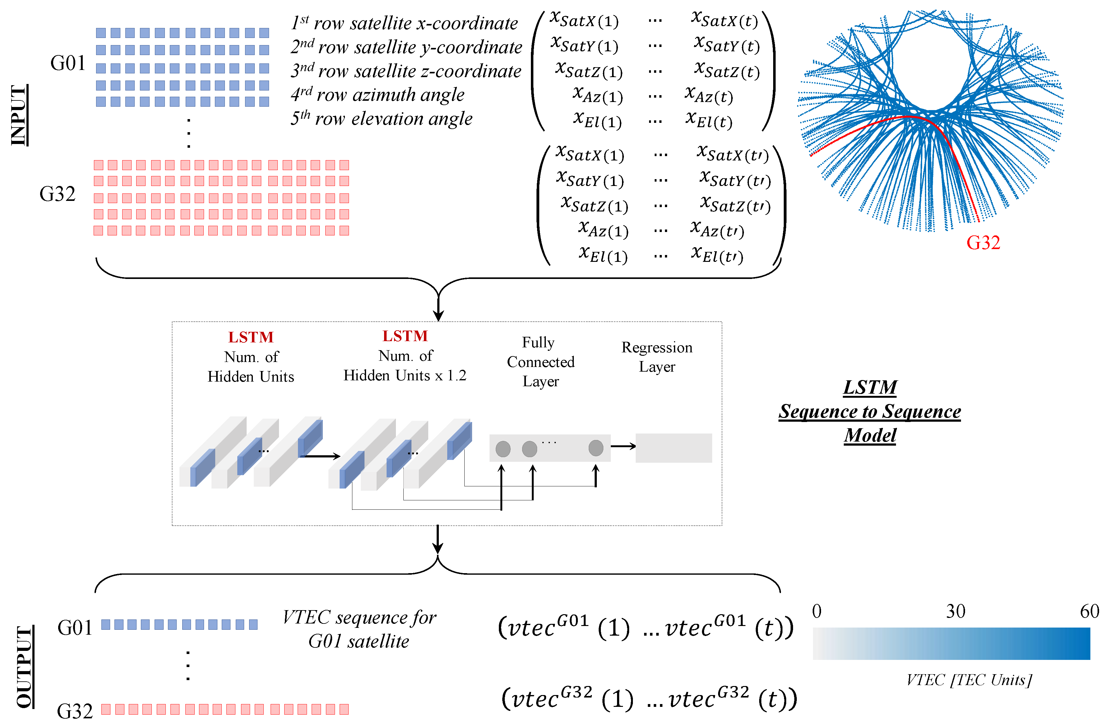
Figure 3 shows the adopted strategy and the basic structure of the proposed LSTM model. The network configuration setup consists of: (i) the input layer, (ii) two stacked unidirectional LSTM layers and (iii) the regression layer. In our case, we have a sequence-to-sequence model, in which data are organized as sequences of input and output pairs. This implies that LSTM model infers the relative time information during training, as it is not trained for every pair (input features, output) at every epoch t individually, but is trained to recognize a whole sequence/set of these pairs during the day, for a specific satellite. Thus, the input layer receives the current data in a sequence-like form, of a time window with varying duration. The network includes two bidirectional LSTM layers: the first layer consists of 60 filters with a kernel size 1 × 5, while the second layer consists of 72 filters of the same kernel size. The regression layer consists of one fully connected hidden layer and the final output regression layer. The output is a sequence of VTEC predicted values for each satellite, with size that covers the whole duration where the satellite is visible from the receiver.
In order to evaluate the ionospheric delay effects on GPS positioning, days between 10 and 13 December 2018 (day of year (DOY), from 344 to 347), where 80 % of them has selected for training and the remaining 20 % as validation set. Furthermore, 10 days have been selected as test set (14 December and 19 to 27 December 2018). Thus, we feed our network with the sequence-pairs (Figure 3):
( x ) T R A I N = x S a t X ( 1 ) x S a t X ( 2 ) x S a t X ( t ) x S a t Y ( 1 ) x S a t Y ( 2 ) x S a t Y ( t ) x S a t Z ( 1 ) x S a t Z ( 2 ) x S a t Z ( t ) x A z ( 1 ) x A z ( 2 ) x A z ( t ) x E l ( 1 ) x E l ( 2 ) x E l ( t ) a n d ( v t e c ) T R A I N = v t e c ( 1 ) v t e c ( 2 ) v t e c ( t )
after training has been completed, we test the model providing the ( x ) T E S T values and expecting the outcome ( v t e c ) T E S T .

3. PPP Processing Strategy

This section describes the pre-processing strategy to extract the necessary inputs and outputs for our LSTM model, using observational data from a small group of permanent GNSS stations in the IGS network. The evaluation of the LSTM method for vectical TEC values prediction has been conducted on various ground stations of the global network of International GNSS Service (IGS). The time resolution is selected to be 30s. Table 1 shows the geographical distribution of the six selected IGS stations [40], which are spread across central Europe and are located in close proximity to each other.
We used the GAMP software [31], a secondary development software based on RTKLIB [41] for multi-constellation and multi-frequency Precise positioning. GAMP allows the use of undifferenced and uncombined observations in dual-frequency PPP processing to extract STEC values. Using the uncombined PPP (UPPP) model allows estimating the ionospheric effects as unknown parameters, without the need to impose ionospheric-free constraints imposed by the traditional PPP model which amplifies the measurement noise when dual frequency observations are combined to cancel the ionospheric effects. The necessary RINEX observation and navigation files, along with precise orbit and clock information, IGS ANTEX (igs14.atx) and SINEX files, as well as ocean tide loading coefficients and DCBs are entered into the GAMP software for static PPP processing. Wuhan University’s satellite orbits and clock offsets were provided as input for GAMP software. Differential code biases (DCBs), are essential in many navigation and non-navigation applications (such as ionospheric analysis). As new signals are currently provided by the modernized GNSS systems, the need for a comprehensive multi-GNSS DCB product arises. DCB products, as part of the IGS Multi-GNSS Experiment (MGEX), are provided by the Chinese Academy of Sciences (CAS) in Wuhan (Table 2).

4. Results and Discussion

4.1. Performance Comparison among Different Methods

We compare the proposed LSTM method against traditional stochastic models for timeseries modeling and forecasting, such as the autoregressive AR model and the autoregressive moving average ARMA model. Our LSTM model has been trained and deployed using Python with Tensorflow and Keras libraries. We trained the model using the adaptive moment estimation optimization algorithm (adam) with a learning rate of 10 4 . Model weights and coefficients are updated using a mini-batch size of 28 samples at each training iteration. The maximum number of epochs for training is selected to be 600. Deep learning performance is improved through data balance and normalization of the data used as input to the LSTM network to the range [ 0 , 1 ] . We have individual networks, one per station. AR and ARMA models were also implemented in Python using the stats models library.
m a e ¯ r = 1 S s i = 1 S M A E r s i = 1 S s i = 1 S t = 1 T v t e c r , t s i v t e c ^ r , t s i T
m i n ¯ r = 1 S s i = 1 S ( min t T ( v t e c r , t s i v t e c ^ r , t s i ) )
m a x ¯ r = 1 S s i = 1 S ( max t T ( v t e c r , t s i v t e c ^ r , t s i ) )
r m s e ¯ r = 1 S s i = 1 S R M S E r s i = 1 S s i = 1 S 1 T 1 t = 1 T ( v t e c r , t s i v t e c ^ r , t s i ) 2
Table 3 shows performance metrics between LSTM model, as well as ARMA and AR models. For each satellite s i in every station r, a sequence of VTEC values is produced using the TEC model, for a given time period T. For each individual satellite, we compute the absolute difference between the ground truth v t e c ^ r , t s i value, as obtained from the processing with the GAMP software, and the estimated from our model v t e c r , t s i value, thus we have the difference v t e c r , t s i v t e c ^ r , t s i , every time/epoch.
For every station r, we have also computed two additional metrics for every individual PRN ( s i -satellite): the mean absolute error M A E r s i (i.e., the average sum of all absolute errors) and the root mean squared error R M S E r s i . However, Table 3 summarizes an overall accuracy for each station, using the following performance metrics: (i) m a e ¯ r is the average value of the combined M A E r s i for all s i satellite estimations per station, (ii) m i n ¯ r is the average of all s i minimum difference values per station, (iii) in accordance to m i n ¯ r metric, m a x ¯ r is the average of all s i maximum differences values per station, and (iv) r m s e ¯ r is the average of s i root mean squared error of all PRNs (satellites) per station. LSTM, ARMA ans AR are causal models, thus they are appropriate for ionospheric time series modeling. However, our proposed unidirectional LSTM model performs best (Table 3) mainly due to its capability to effectively identify structure and pattern of TEC data, such as non-linearity and complexity in time series prediction and infer TEC behavior based on previous states.
LSTM model is undoubtedly, more complicated and difficult to train and in most cases does not exceed the performance of a simple ARMA model. Table 4 shows the computational time required for model training by each method. Evidently, in terms of computational load, the AR model requires the minimum time (1 s) for training, while LSTM is the most time-consuming model (>600 s), but this is to be anticipated mainly due to its complexity and its large number of trainable parameters. However, by inspecting the various statistical metrics, it can also be seen that the LSTM model achieves the best performance in terms of its agreement with the conventional GNSS-derived VTEC data.

4.2. Comparison among Different Stations and Time Periods

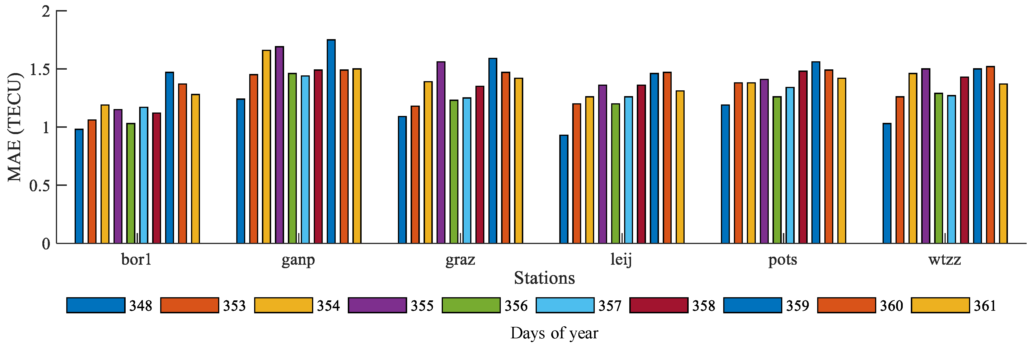
Figure 4 illustrates the m a e ¯ r metric for a testing period of 10 days, for the 6 different stations. MAE values ranging from 0.9 to 1.5 TECU. The ’ganp’ station shows the worse values with low accuracy, while ’bor1’ station achieves the highest accuracy among the other stations. Regarding the test period, the results are quite similar, however we observe a slightly increasing trend in MAE error, which is to be expected, as the predictions are carried out further away from the training period of the LSTM model.

4.3. Comparison between Different Satellites

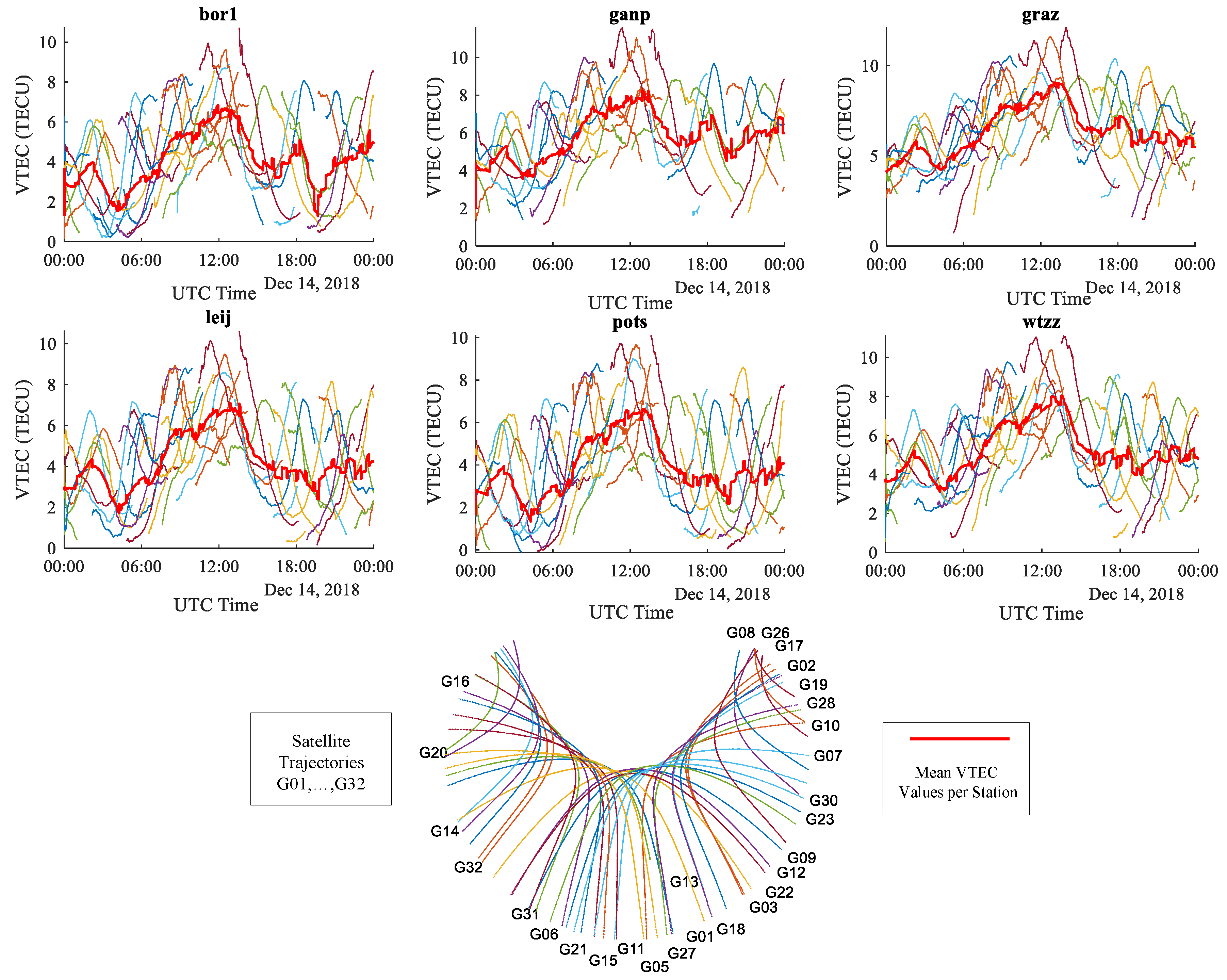
In order to gain a further insight into the LSTM’s model performance, we evaluated the VTEC prediction performance for each satellite. Figure 5 shows the estimated VTEC values for each station, per satellite on December 14, 2018. As noted, VTEC values show significant variation during the day, depending on the electron density in the ionosphere. The ionospheric delay changes slowly through a daily cycle, exhibiting its minimum values (2–4 TECU) between midnight and early morning, and reaching its peak (6–8 TECU) during the daylight hours, in the mid-latitudes.
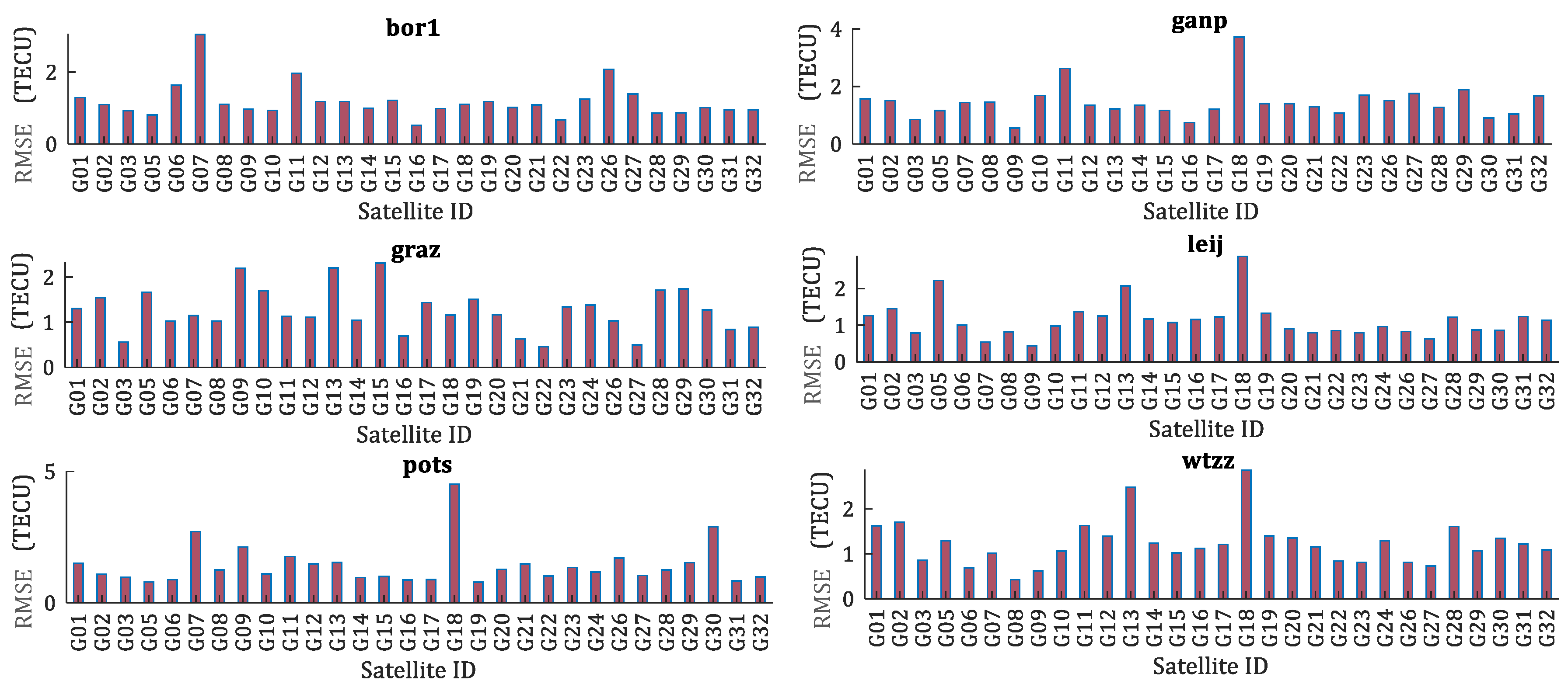
As a next step, we evaluated the LSTM model’s performance using the root mean squared error (RMSE) metric of VTEC values for each visible satellite, in a bar graph format. In general, RMSE TEC values are ranging between 0.5 and 2 TECU for each reference station (Figure 6). For station ‘bor1’, the highest RMSE values are observed for G07, G26 and G11 satellites in view. For station ‘ganp’, G18 and G11 show the highest error values. Station ‘graz’ exhibits significant variation between the satellites’ RMSE values, with the satellites G15, G13 and G09 showing the maximum RMSE TEC values. Station ‘leij’ RMSE VTEC values reach the maximum for satellites G18 and G05. Satellite G18 has also the maximum RMSE for the other two remaining stations ‘pots’ and ‘wtzz’.
In particular, Figure 7 shows the predicted LSTM-aided vertical TEC values for each one of the GPS satellites (when they are visible from ‘bor1’ station), along with the vertical TEC values being derived from GAMP software (ground truth data). As noted, LSTM model can adequately predict VTEC’s model performance for every satellite separately. The satellites G07, G11 and G26 have the worst performance, as expected, based on results from Figure 6. On the contrary, the satellites G05, G16 and G22 have the best performance in VTEC prediction.

4.4. Comparison among Different Ionosphere Models

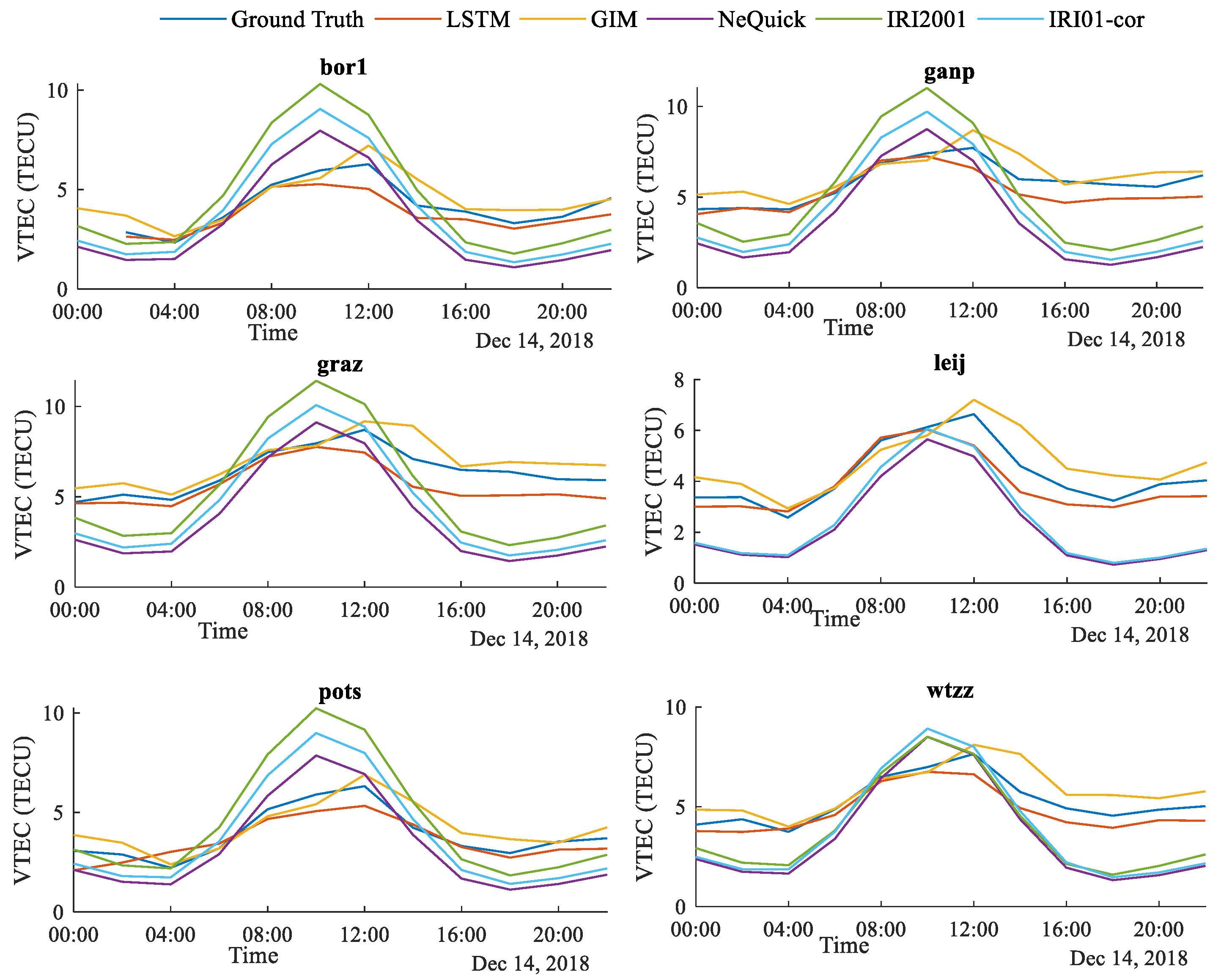
To further analyze the LSTM model’s performance, Figure 8 shows the mean VTEC values at every station, as obtained from NeQuick, IRI2001, IRI01-cor and GIM TEC estimates compared to the GPS-based TEC and LSTM TEC predictions, during the day. The VTEC maxima is appeared for all stations between 8:00 and 12:00 a.m. In most cases, LSTM predicted values are similar to GPS TEC derived values, however, it is noted that our model underestimates VTEC values, showing lower values than those of GPS TEC. GIM-aided TEC values are also close to LSTM derived TEC values. NeQuick, IRI2001 and IRI01-cor values show greater variability during the day with higher maximum and lower minimum than those of GPS TEC and GIM values.
Figure 9 shows the mean difference values having as base GPS TEC estimates. As noted, in most cases LSTM predictions are closer to GPS TEC estimates, as they have small difference, except for station ‘graz’, where GIM model’s estimates seem to have a slightly better performance.

5. Conclusions

We propose a supervised, unidirectional regression LSTM model for efficient prediction of vertical TEC values. Typical and widely used AR and ARMA models are linear models, suitable for TEC prediction, as ionosphere exhibits periodic changes. Thus, the AR and ARMA models’ autoregressive character offers an advantage in VTEC prediction. However, the additional inclusion of selected features (such as the satellite vector, and the satellite elevation and azimuth) in the supervised LSTM algorithm, as well as, the fact that LSTM networks are equipped with memory cell and consequently they are able to preserve the worth-remembering information content in the input STEC data, gives superiority and an extra boost to our proposed method. Non-linearity and long-term prediction are additional advantages of our proposed LSTM method. As next steps, we intend to direct our studies into investigating the performance of this LSTM model under typical non-quiet conditions, including data from periods with intense ionospheric activity (e.g., periods with ionosphere anomalies and disturbances), and explore the possibility of using, with appropriate expansions, our LSTM model as a tool capable of adapting its performance to detect/catch extreme ionosphere conditions. To this end, alternative recurrent neural network methods, such as bidirectional LSTMs, that introduce non-causality, should be explored or/and check the performance of advanced Convolutional Neural Network (CNN) -based methods and how they can be optimally adapted in timeseries prediction problems for further benefit of the variant PPP techniques. In addition, we intend to explore models’ behavior in datasets consisting of multiple GNSS constellations (such as GLONAS, Galileo, etc.).

Author Contributions

Concectualization, M.K., A.V. and D.D.; Supervision, Athanasios Voulodimos, N.D. and A.D.; Visualization, M.K.; Writing original draft, M.K.; Writing review and edititng, A.V., N.D., A.D. and D.D. All authors have read and agreed to the published version of the manuscript.

Funding

This research is co-financed by Greece and the European Union (European Social Fund- ESF) through the Operational Programme “Human Resources Development, Education and Lifelong Learning” in the context of the project “Strengthening Human Resources Research Potential via Doctorate Research” (MIS-5000432), implemented by the State Scholarships Foundation (IKY).

Conflicts of Interest

The authors declare no conflict of interest.

Abbreviations

The following abbreviations are used in this manuscript:
ARAutoregressive
ARMAAutoregressive Moving Average
CASChinese Academy of Sciences
CODECentre for Orbit Determination in Europe
CNNConvolutional Neural Networks
DCBDifferential Code Biases
COSPARCommittee On Space Research
DOYDay of Year
ESAEuropean Space Agency
GIMGlobal Ionosphere Maps
GNSSGlobal Navigation Satellite System
IAACIonosphere Associate Analysis Center
IGGInstitute of Geodesy and Geophysics
IGSInternational GNSS Service
IONEXIONospheric EXchange
JPLJet Propulsion Laboratory
LSTMLong Short-Term Memory
MGEXMulti-GNSS Experiment
RBFRadial Basic Function
RNNRecurrent neural network
STECSlant Total Electron Content
TECTotal electron content
UPCPolytechnic University of Catalonia
URSIUnion of Radio Science
VBLIVery Long Baseline Interferometry
VTECVertical Total Electron Content

References

  1. Hoque, M.M.; Jakowski, N. Higher Order Ionospheric Effects in Precise GNSS Positioning. J. Geodesy 2007, 81, 259–268. [Google Scholar] [CrossRef]
  2. Klobuchar, J. Ionospheric time-delay algorithm for single frequency GPS users. IEEE Trans. Aerosp. Electron. Syst. 1987, 23, 325–332. [Google Scholar] [CrossRef]
  3. Nava, B.; Coïsson, P.; Radicella, S. A New Version of the NeQuick Ionosphere Electron Density Model. J. Atmos. Solar-Terrestrial Phys. Ionos. Effects Telecommun. 2008, 15, 1856–1862. [Google Scholar] [CrossRef]
  4. Bakker, P.; Christian, T. Real-Time Multi-GNSS Single-Frequency Precise Point Positioning. GPS Solut. 2017, 4, 1791–1803. [Google Scholar] [CrossRef] [Green Version]
  5. Hochreiter, S.; Jürgen, S. Long Short-Term Memory. Neural Comput. 1997, 8, 1735–1780. [Google Scholar] [CrossRef]
  6. Wang, C.; Xin, S.; Liu, X.; Shi, C.; Fan, L. Prediction of global ionospheric VTEC maps using an adaptive autoregressive model. Earth Planets Space 2018, 70, 18. [Google Scholar] [CrossRef] [Green Version]
  7. Mandrikova, O.V.; Glushkova, N.V.; Zhivet’ev, I.V. Modeling and analysis of ionospheric parameters by a combination of wavelet transform and autoregression models. Geomagn. Aeron. 2014, 54, 593–600. [Google Scholar] [CrossRef]
  8. Voulodimos, A.; Doulamis, N.; Doulamis, A.; Protopapadakis, E. Deep Learning for Computer Vision: A Brief Review. Comput. Intell. Neurosci. 2018, 2018, 7068349. [Google Scholar] [CrossRef]
  9. Protopapadakis, E.; Voulodimos, A.; Doulamis, A.; Doulamis, N.; Dres, D.; Bimpas, M. Stacked Autoencoders for Outlier Detection in Over-the-Horizon Radar Signals. Comput. Intell. Neurosci. 2017, 2017, 5891417. [Google Scholar] [CrossRef]
  10. Greff, K.; Srivastava, R.K.; Koutník, J.; Steunebrink, B.R.; Schmidhuber, J. LSTM: A Search Space Odyssey. IEEE Trans. Neural Netw. Learn. Syst. 2017, 10, 2222–2232. [Google Scholar] [CrossRef] [Green Version]
  11. Jiang, H.; Liu, J.; Wang, Z.; An, J.; Ou, J.; Liu, S.; Wang, N. Assessment of spatial and temporal TEC variations derived from ionospheric models over the polar regions. J. Geod. 2019, 93, 455. [Google Scholar] [CrossRef]
  12. An, X.; Meng, X.; Chen, H.; Jiang, W.; Xi, R.; Chen, Q. Modelling Global Ionosphere Based on Multi-Frequency, Multi-Constellation GNSS Observations and IRI Model. Remote Sens. 2020, 12, 439. [Google Scholar] [CrossRef] [Green Version]
  13. Wang, J.; Huang, G.; Zhou, P.; Yang, Y.; Zhang, Q.; Gao, Y. Advantages of Uncombined Precise Point Positioning with Fixed Ambiguity Resolution for Slant Total Electron Content (STEC) and Differential Code Bias (DCB) Estimation. Remote Sens. 2020, 12, 304. [Google Scholar] [CrossRef] [Green Version]
  14. Krypiak-Gregorczyk, A.; Wielgosz, P.; Borkowski, A. Ionosphere Model for European Region Based on Multi-GNSS Data and TPS Interpolation. Remote Sens. 2017, 9, 1221. [Google Scholar] [CrossRef] [Green Version]
  15. Ren, X.; Zhang, X.; Xie, W.; Zhang, K.; Yuan, Y.; Li, X. Global Ionospheric Modelling using Multi-GNSS: BeiDou, Galileo, GLONASS and GPS. Sci. Rep. 2007, 6, 33499. [Google Scholar] [CrossRef] [PubMed] [Green Version]
  16. Øvstedal, O. Absolute Positioning with Single-Frequency GPS Receivers. GPS Solut. 2002, 5, 33–44. [Google Scholar] [CrossRef]
  17. Alizadeh, M.M.; Wijaya, D.D.; Hobiger, T.; Weber, R.; Schuh, H. Ionospheric Effects on Microwave Signals. In Atmospheric Effects in Space Geodesy; Springer Atmospheric Sciences; Böhm, J., Schuh, H., Eds.; Springer: Berlin/Heidelberg, Germany, 2013. [Google Scholar]
  18. Ou, M.; Zhang, H.; Liu, D.; Yu, X.; Zhen, W. GIM-ingested NeQuick model applied for GPS single frequency ionospheric correction in China. ISAPE 2012 2012, 652–655. [Google Scholar] [CrossRef]
  19. Feng, J.; Han, B.; Zhao, Z.; Wang, Z. A New Global Total Electron Content Empirical Model. Remote Sens. 2019, 11, 706. [Google Scholar] [CrossRef] [Green Version]
  20. Zhang, Z.; Shuguo, P.; Chengfa, G.; Tao, Z.; Wang, G. Support Vector Machine for Regional Ionospheric Delay Modeling. Sensors 2019, 19, 2947. [Google Scholar] [CrossRef] [Green Version]
  21. Huang, Z.; Yuan, H. Ionospheric Single-Station TEC Short-Term Forecast Using RBF Neural Network. Radio Sci. 2014, 49, 283–292. [Google Scholar] [CrossRef]
  22. Yilmaz, A.; Akdogan, K.E.; Gurun, M. Regional TEC Mapping Using Neural Networks. Radio Sci. 2009, 44, 1–16. [Google Scholar] [CrossRef]
  23. Su, K.; Jin, S.; Hoque, M.M. Evaluation of Ionospheric Delay Effects on Multi-GNSS Positioning Performance. Remote Sens. 2019, 11, 171. [Google Scholar] [CrossRef] [Green Version]
  24. Bosco, H.J.; McKinnell, L.; Cilliers, P.J.; Opperman, B. Application of Neural Networks to South African GPS TEC Modelling. Adv. Space Res. 2009, 43, 1711–1720. [Google Scholar]
  25. Boulch, A.; Cherrier, N.; Castaings, T. Ionospheric Activity Prediction Using Convolutional Recurrent Neural Networks. arXiv 2018, arXiv:1810.13273. [Google Scholar]
  26. Sun, W.; Xu, L.; Huang, X.; Zhang, W.; Yuan, T.; Yan, Y. Bidirectional LSTM for ionospheric vertical Total Electron Content (TEC) forecasting. In Proceedings of the 2017 IEEE Visual Communications and Image Processing (VCIP), St. Petersburg, FL, USA, 10–13 December 2017; pp. 1–4. [Google Scholar]
  27. Sundermeyer, M.; Schlüter, R.; Ney, H. LSTM Neural Networks for Language Modeling. In Proceedings of the INTERSPEECH, Portland, OR, USA, 9–13 September 2012. [Google Scholar]
  28. Graves, A.; Mohamed, A.; Hinton, G. Speech Recognition with Deep Recurrent Neural Networks. In Proceedings of the IEEE International Conference on Acoustics, Speech and Signal Processing, Vancouver, BC, Canada, 26–31 May 2013; pp. 6645–6649. [Google Scholar]
  29. Ullah, A.; Ahmad, J.; Muhammad, K.; Sajjad, M.; Baik, S.W. Action Recognition in Video Sequences Using Deep Bi-Directional LSTM With CNN Features. IEEE Access 2018, 6, 1155–1166. [Google Scholar] [CrossRef]
  30. Graves, A. Generating Sequences With Recurrent Neural Networks. arXiv 2014, arXiv:1308.0850. [Google Scholar]
  31. Zhou, F.; Dong, D.; Li, W.; Jiang, X.; Wickert, J.; Schuh, H. GAMP: An open-source software of multi-GNSS precise point positioning using undifferenced and uncombined observations. Gps Solut. 2018, 22, 33. [Google Scholar] [CrossRef]
  32. Xiang, Y.; Gao, Y.; Li, Y. Ionospheric stec and vtec constraints for fast ppp. In China Satellite Navigation Conference; Springer: Singapore, 2017; pp. 257–269. [Google Scholar]
  33. Komjathy, A.; Langley, R.B. An assessment of predicted and measured ionospheric total electron content using a regional GPS network. In Proceedings of the ION National Technical Meeting, Santa Monica, CA, 22–24 January 1996; pp. 615–624. [Google Scholar]
  34. Abdelazeem, M.; Çelik, R.N.; El-Rabbany, A. An efficient regional ionospheric model using combined GPS/BeiDou observations. J. Spat. Sci. 2017, 62, 323–335. [Google Scholar] [CrossRef]
  35. Rho, H.; Langley, R.B.; Komjathy, A. An enhanced UNB ionospheric modeling technique for SBAS: The quadratic approach. In Proceedings of the 17th International Technical Meeting of the Satellite Division of the Institute of Navigation, Long Beach, CA, USA, 21–24 September 2004; pp. 354–365. [Google Scholar]
  36. Brunini, C.; Azpilicueta, F. GPS slant total electron content accuracy using the single layer model under different geomagnetic regions and ionospheric conditions. J. Geod. 2010, 84, 293–304. [Google Scholar] [CrossRef]
  37. Xiang, Y.; Gao, Y. An Enhanced Mapping Function with Ionospheric Varying Height. Remote Sens. 2019, 11, 1497. [Google Scholar] [CrossRef] [Green Version]
  38. Doulamis, A.D.; Doulamis, N.D.; Kollias, S.D. An Adaptable Neural-Network Model for Recursive Nonlinear Traffic Prediction and Modeling of MPEG Video Sources. IEEE Trans. Neural Netw. 2003, 14, 150–166. [Google Scholar] [CrossRef]
  39. Gers, F.A.; Schmidhuber, J.; Cummins, F. Learning to Forget: Continual Prediction with LSTM. In 1999 Ninth International Conference on Artificial Neural Networks ICANN; IET: London, UK, 1999. [Google Scholar]
  40. Montenbruck, O.; Steigenberger, P.; Prange, L.; Deng, Z.; Zhao, Q.; Perosanz, F.; Romero, I.; Noll, C.; Stürze, A.; Weber, G. The Multi-GNSS Experiment (MGEX) of the International GNSS Service (IGS)—Achievements, Prospects and Challenges. Adv. Space Res. 2017, 59, 1671. [Google Scholar] [CrossRef]
  41. Kaselimi, M.; Doulamis, N.; Delikaraoglou, D.; Protopapadakis, E. GNSSGET and GNSSPLOT Platforms–Matlab GUIs for Retrieving GNSS Products and Visualizing GNSS Solutions. In Proceedings of the 13th International Joint Conference on Computer Vision, Imaging and Computer Graphics Theory and Applications (VISIGRAPP 2018)-VISAPP, Funchal, Madeira, Portugal, 27–29 January 2018; Volume 5, pp. 626–633. [Google Scholar]
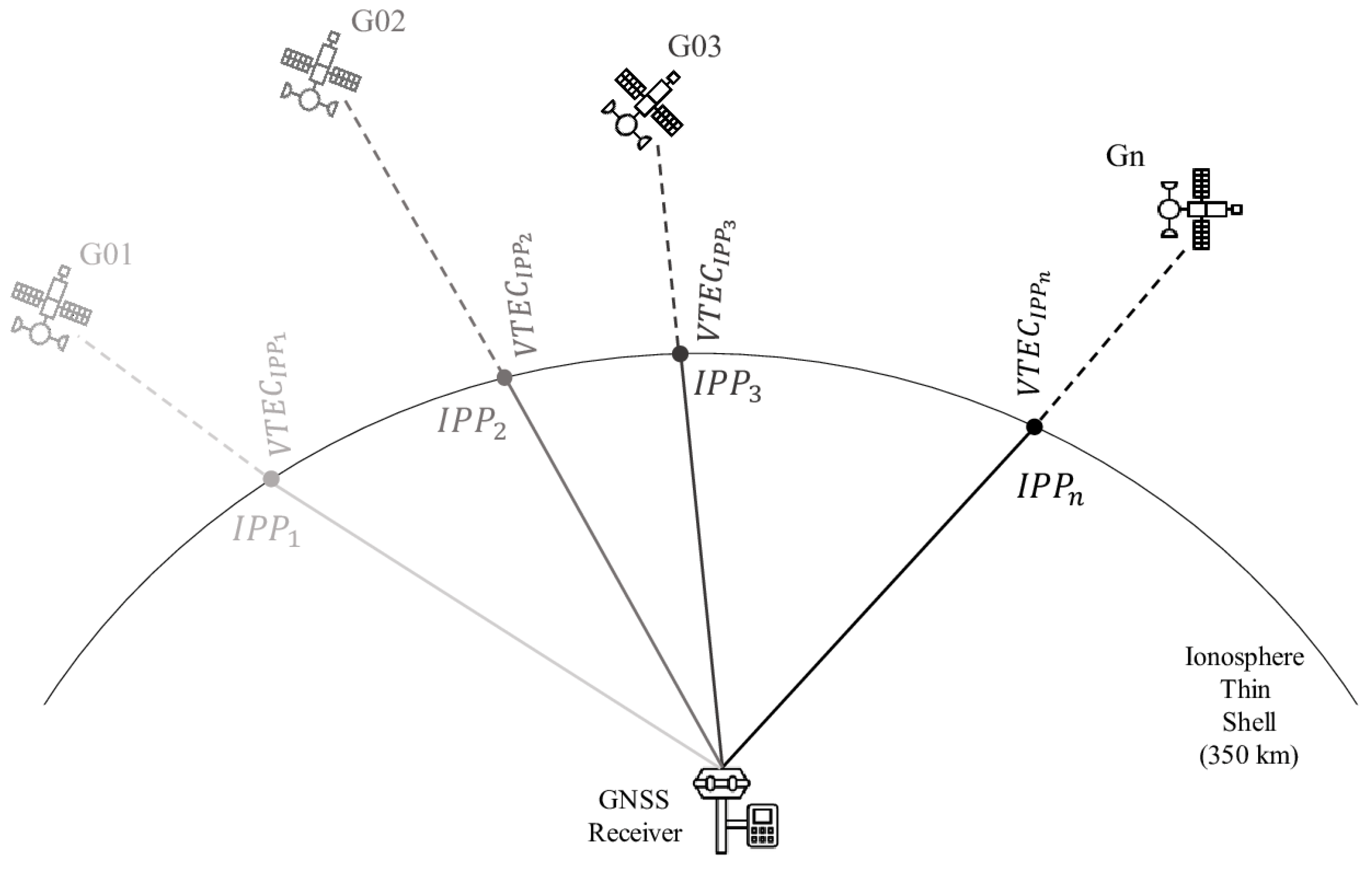
Figure 1. VTEC variations per individual PRN, at a specific time epoch. IPP points are the intersections of GNSS signal in the ionosphere assuming the theory of single layer model (SLM). Based on the assumption that adjacent points share the same ionosphere conditions, our model investigates GNSS method’s efficiency in providing TEC estimations.
Remotesensing 12 01354 g001
Figure 2. The memory cell of an LSTM network. It contains three different components; (i) the forget gate f(t), (ii) the input gate i(t) and the input node g(t) and (iii) the output node o(t) (right). Unidirectional LSTM regression model used for TEC estimation (left).
Remotesensing 12 01354 g002
Figure 3. This proposed LSTM architecture for TEC sequence ( v t e c s ( 1 ) ... v t e c s ( t ) ) prediction. The deep learning structure consists of two stacked LSTM layers. The proposed LSTM is a sequence to sequence regression model. The output is TEC sequences from GNSS observations at a given station which are of varying length (e.g., t, t’) and the input has as features the satellite position vector [ x S a t X x S a t Y x S a t Y ], the azimuth ( x A z ) and the elevation angles x E l of the satellite direction from the receiver site. For example satellite G32 with a trajectory as illustrated in the figure with red line, is visible from station bor1 for about 5 h, thus the input sequence for G32 satellite has length 600 values, for the measurements sampling rate at 30 s.
Remotesensing 12 01354 g003
Figure 4. MAE error per station for 10 different days.
Remotesensing 12 01354 g004
Figure 5. VTEC (TECU) predictions on 14 December 2019 for six stations (bor1, ganp, graz, leij, pots, wtzz) per satellite ID (G1,..., G32 for GPS satellite), and mean VTEC value (with red line).
Remotesensing 12 01354 g005
Figure 6. Root Mean Squared Error (RMSE) metric of the VTEC(TECU) predictions using LSTM method per station (bor1, grap, graz, leij, pots, wtzz) and per satellite ID (G1,.., G32 for GPS constellation).
Remotesensing 12 01354 g006
Figure 7. Vertical TEC of each GPS satellite between the GPS ground truth values and our LSTM method’s results on 14 December 2018, for ’bor1’ station.
Remotesensing 12 01354 g007
Figure 8. Comparison between VTEC (TECU) LSTM predictions (PRD), estimated GPS ionospheric VTEC values (GRD) and the VTEC models (GIM, NeQuick, IRI2001 and IRI01-cor).
Remotesensing 12 01354 g008
Figure 9. Mean difference between the estimated GPS VTEC values and the VTEC (TECU) LSTM predictions (LSTM), GIM VTEC model values, NeQuick VTEC model values, IRI2001 VTEC model values and IRI01-cor VTEC model values.
Remotesensing 12 01354 g009
Table 1. Approximate location of six selected stations of IGS network and the countryt of their origin.
StationsLatitude°Longitude°Country
bor152.27695835217.073459989Poland
ganp49.03471504420.322939096Slovakia
graz47.06713159515.493484133Austria
leij51.35398198012.374101226Germany
pots52.37929910913.066095112Germany
wtzz49.14421397712.878907414Germany
Table 2. Static PPP experimental setup.
OptionsSettings
ConstellationGPS
Positioning modestatic PPP
FrequenciesL1, L2
Sampling rate30 s
Elevation mask 7
Differential code bias (DCB)Correct using MGEX DCB products for PPP
Tropospheric zenith wet delayinitial model + estimated (random walk process)
Receiver and Satellite antennacorrected with igs14.atx
Phase wind-upCorrected
Sagnac effect, relativistic effectCorrected with IGS absolute
Station reference coordinatesIGS SINEX solutions
Table 3. Performance metrics (mean, minimum (Min), maximum (Max) and root mean squared error (rmse)) for VTEC (TECU) prediction for six selected stations (bor1, ganp, graz, leij, pots and wtzz) among the proposed solution (LSTM) and two other commonly used methods (ARMA, AR).
Receiver r bor1 ganp graz
Metric mae ¯ r min ¯ r max ¯ r rmse ¯ r mae ¯ r min ¯ r max ¯ r rmse ¯ r mae ¯ r min ¯ r max ¯ r rmse ¯ r
LSTM0.980.043.051.181.240.022.881.451.090.032.761.26
ARMA1.410.013.761.761.630.023.942.031.700.043.852.03
AR1.910.044.402.291.850.024.282.251.770.023.982.13
Receiver rleijpotswtzz
Metric mae ¯ r min ¯ r max ¯ r rmse ¯ r mae ¯ r min ¯ r max ¯ r rmse ¯ r mae ¯ r min ¯ r max ¯ r rmse ¯ r
LSTM0.930.022.661.141.190.013.521.421.030.042.681.23
ARMA1.630.013.961.981.710.014.122.071.540.013.781.91
AR1.870.014.222.221.940.014.332.301.790.014.102.15
Table 4. Computational time (in s) per method (LSTM, ARMA and AR) for three selected stations (bor1, graz and wtzz).
Elapsed Time (s)
StationsLSTMARMAAR
bor1719551
graz559583
wtzz600531