Implementation of a Surface Water Extent Model in Cambodia using Cloud-Based Remote Sensing


Abstract
1. Introduction
2. Methods
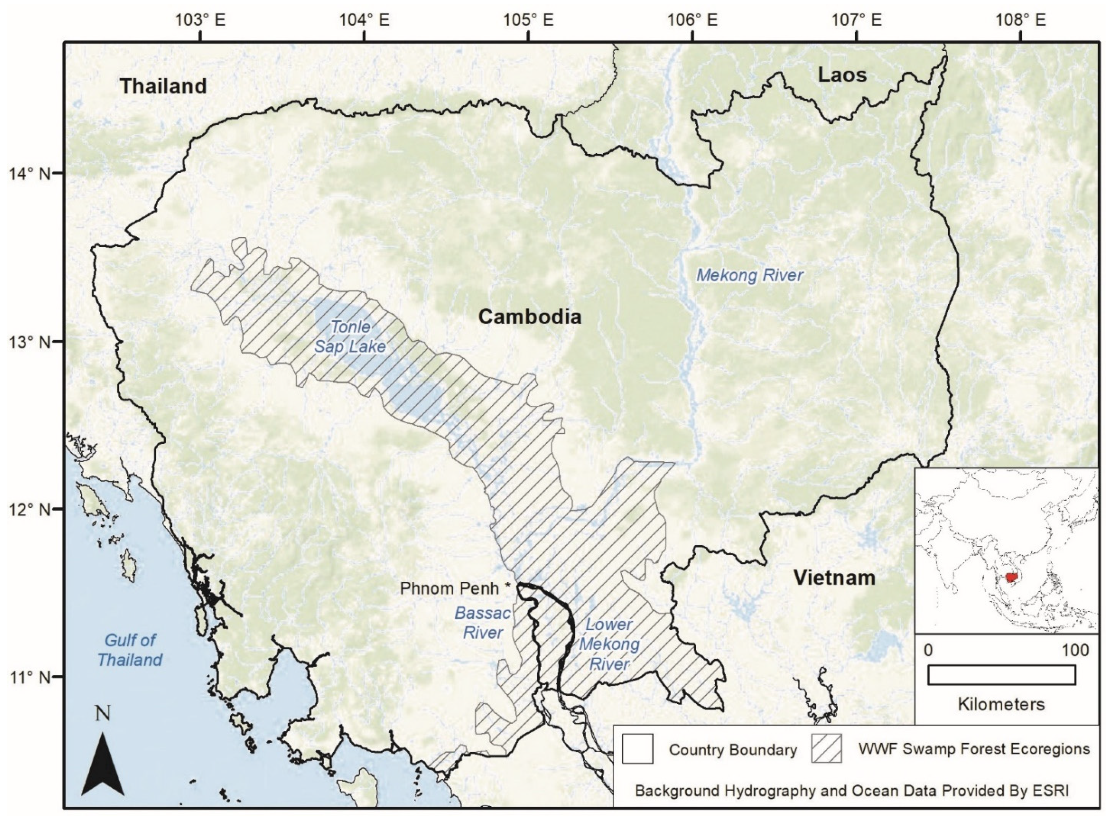
2.1. Study Area
2.2. Generation of Dynamic Surface Water Extent Maps in Google Earth Engine
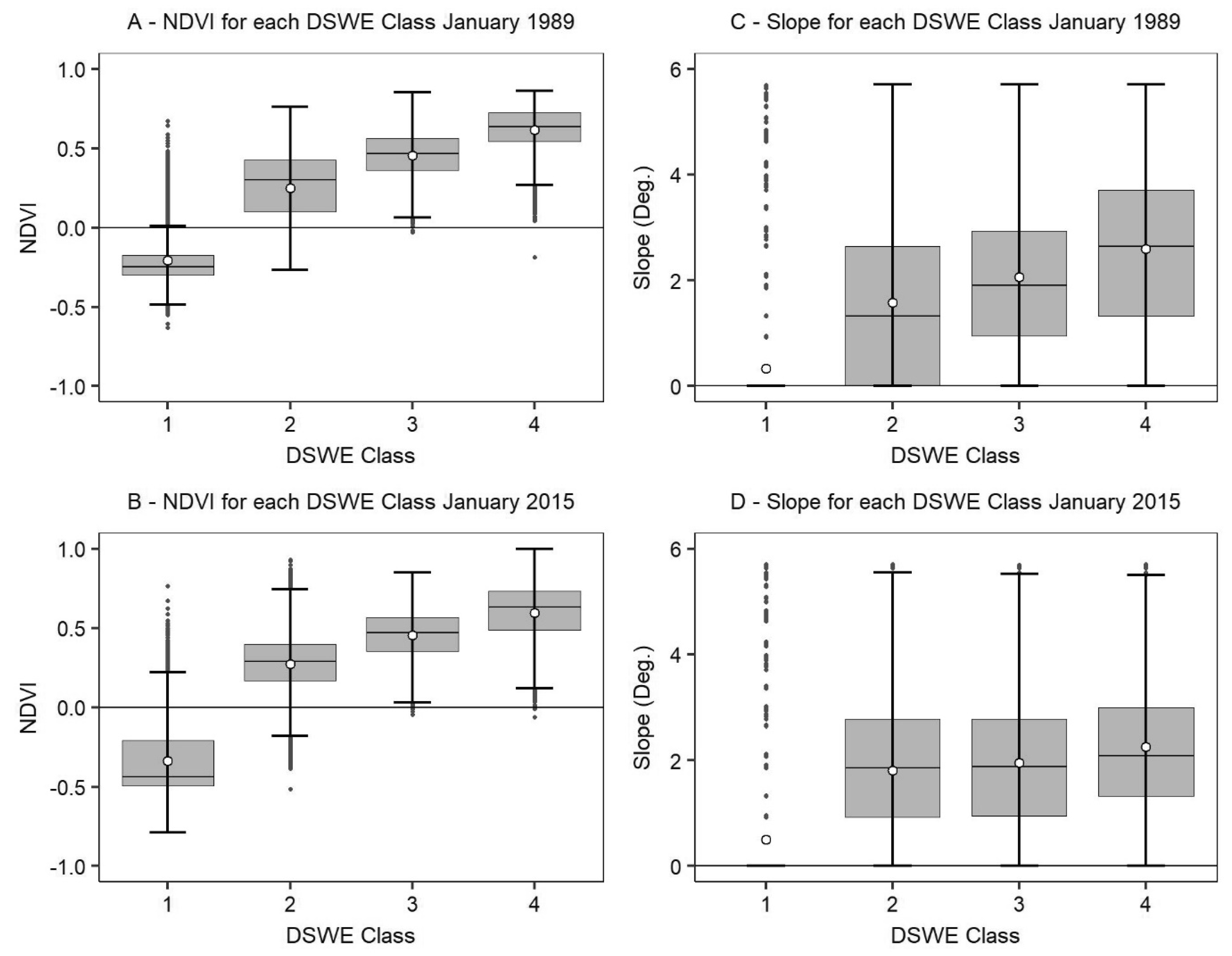
2.3. Comparison of DSWE to NDVI, Slope, and JRC Surface Water Maps
2.4. Multi-Date Accuracy Assessment of DSWE Water Classes
2.5. Exploration of DSWE Class Dynamics
3. Results
3.1. Generation of Monthly and Annual Composite DSWE Products
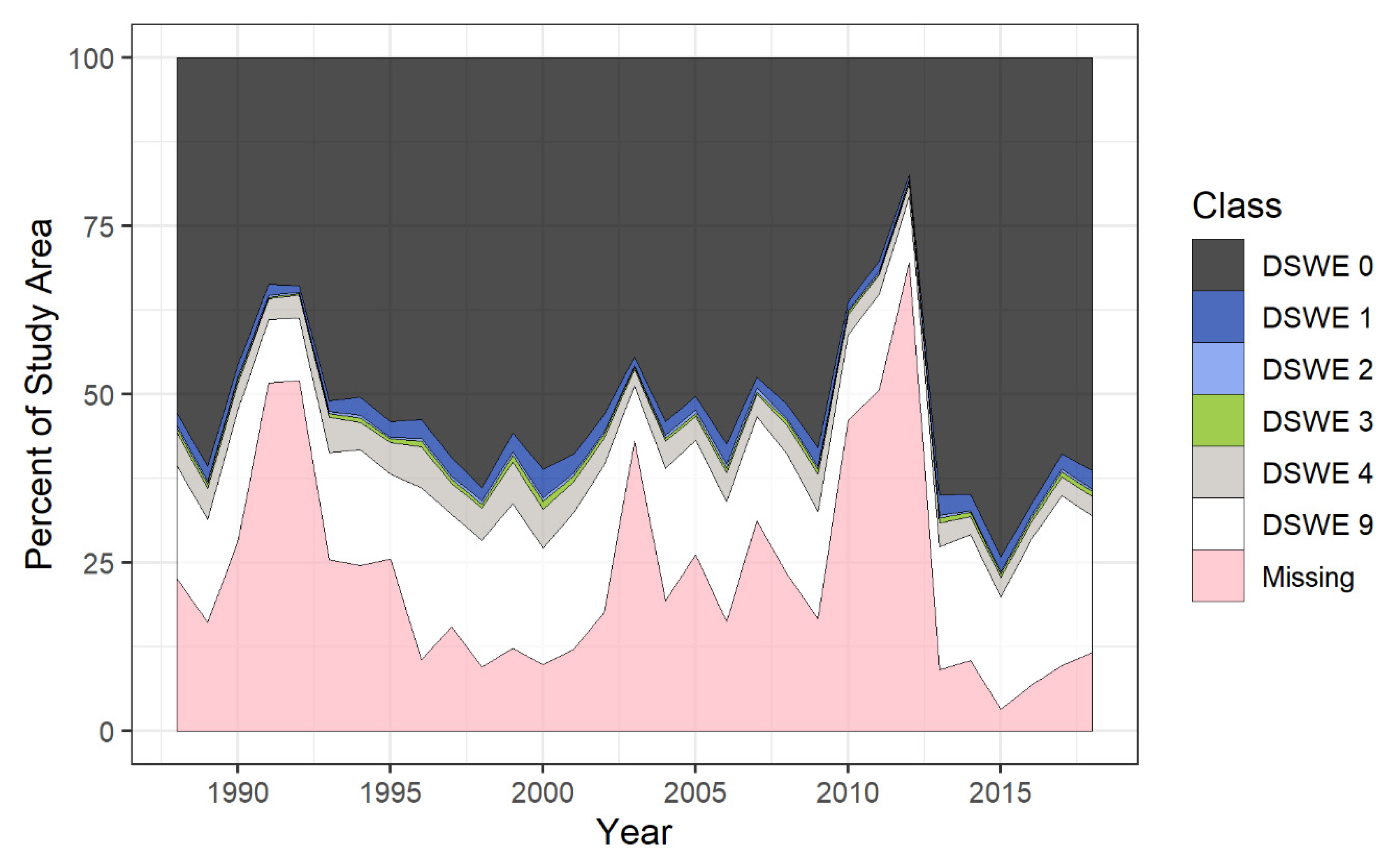
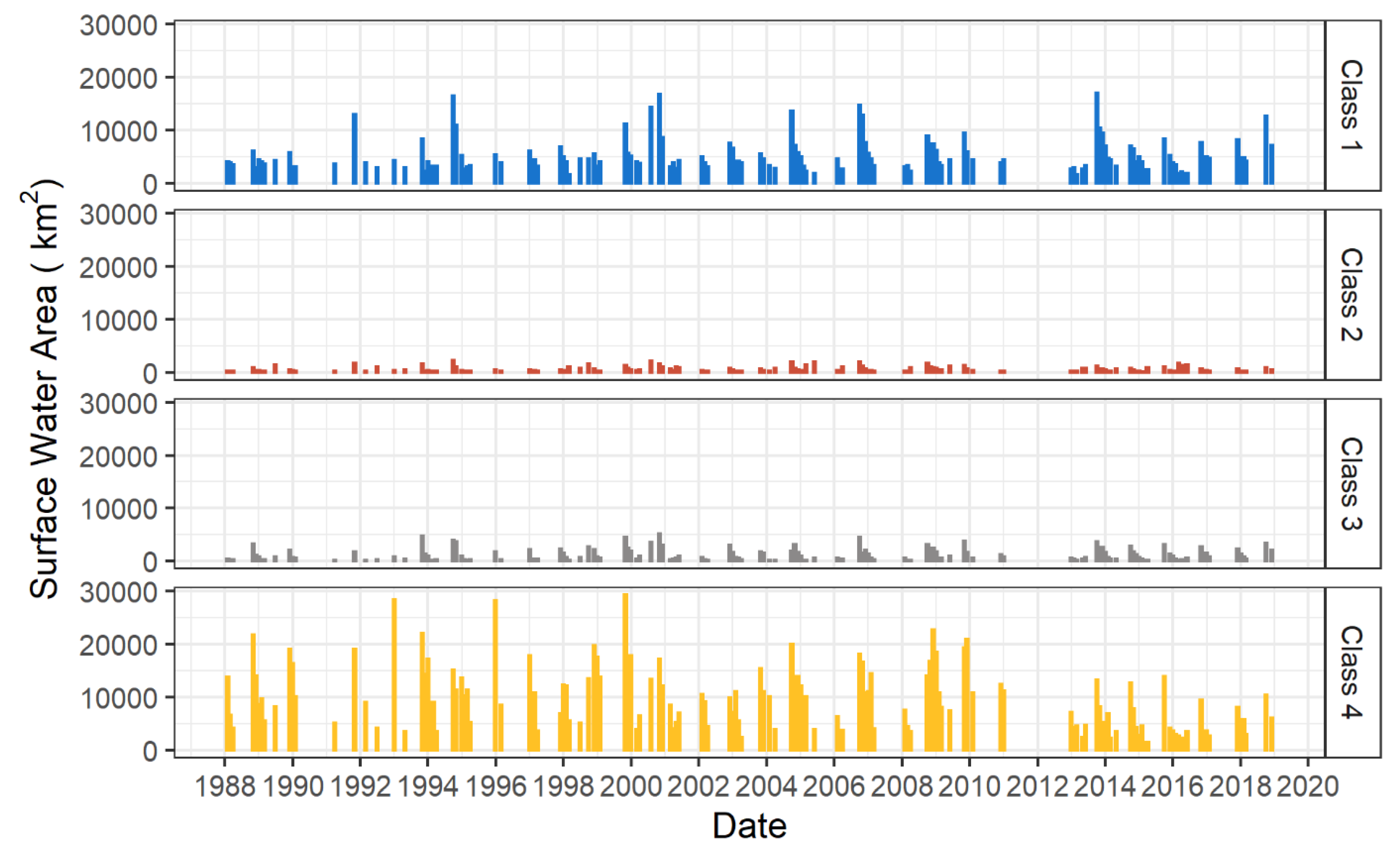
3.2. DSWE Class Dynamics in Cambodia
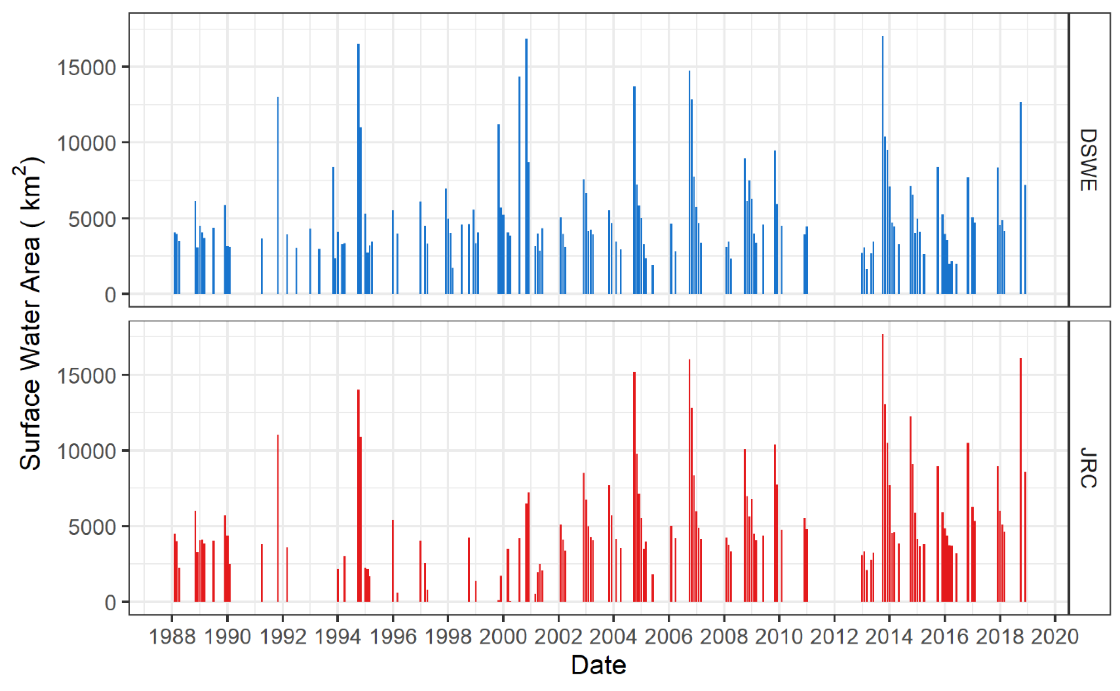
3.3. Comparing DSWE to JRC Maps
3.4. Multi-Date Accuracy Assessment
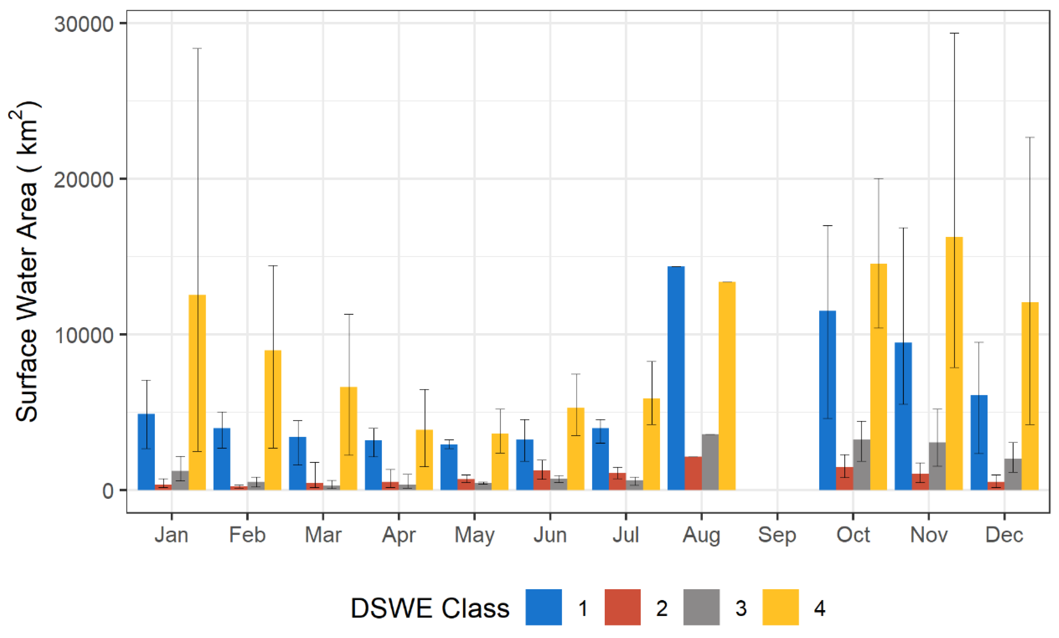
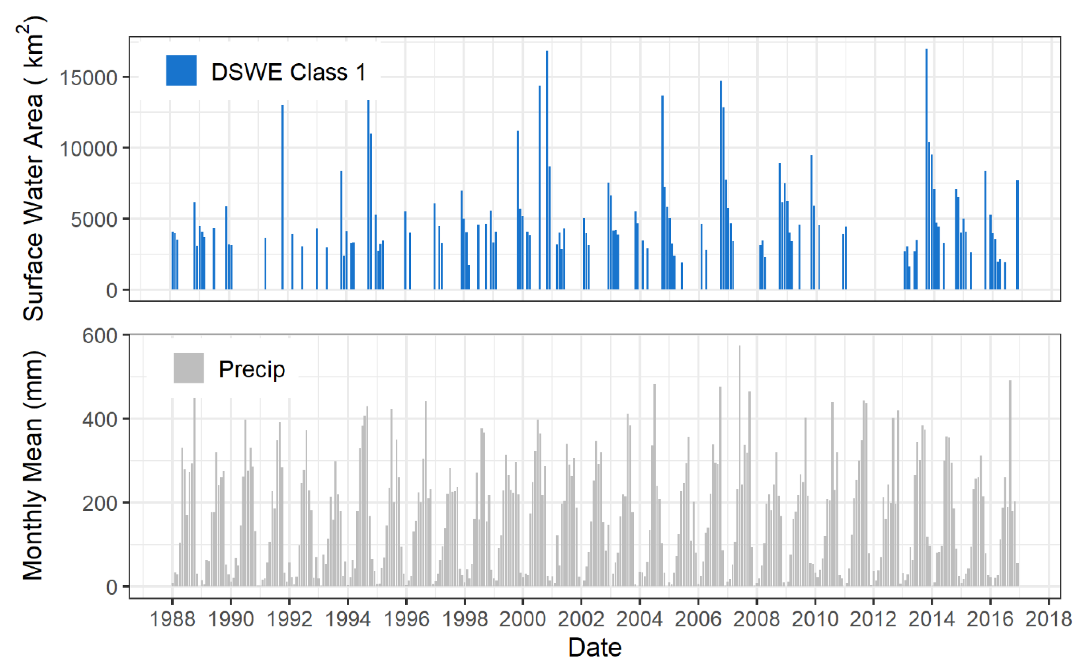
3.5. Annual and Monthly Summary of the “High Confidence” Water Class
4. Discussion
4.1. Discontinuity of the Landsat Record
4.2. Accuracy Assessment
4.3. Future Directions
5. Conclusions
Supplementary Materials
Author Contributions
Funding
Acknowledgments
Conflicts of Interest
References
- Borga, M.; Gaume, E.; Creutin, J.D.; Marchi, L. Surveying flash floods: Gauging the ungauged extremes. Hydrol. Process. 2008, 22, 3883–3885. [Google Scholar] [CrossRef]
- Lettenmaier, D.P. Observations of the Global Water Cycle—Global Monitoring Networks. In Encyclopedia of Hydrological Sciences; Anderson, M.G., McDonnell, J.J., Eds.; John Wiley & Sons, Ltd.: Chichester, UK, 2005. [Google Scholar]
- Moore, R.J.; Cole, S.J.; Bell, V.A.; Jones, D.A. Issues in flood forecasting: Ungauged basins, extreme floods and uncertainty. IAHS Publ. Ser. Proc. Rep. 2006, 305, 103–122. [Google Scholar]
- Carter, R.W.; Davidian, J. General Procedure for Gaging Streams, US Geological Survey. 1968. Available online: https://pubs.usgs.gov/twri/twri3-A6/ (accessed on 2 March 2020).
- Bales, J.D.; Wagner, C.R. Sources of uncertainty in flood inundation maps. J. Flood Risk Manag. 2009, 2, 139–147. [Google Scholar] [CrossRef]
- Beesley, L.; King, A.J.; Amtstaetter, F.; Koehn, J.D.; Gawne, B.; Price, A.; Nielsen, D.L.; Vilizzi, L.; Meredith, S.N. Does flooding affect spatiotemporal variation of fish assemblages in temperate floodplain wetlands? Freshw. Biol. 2012, 57, 2230–2246. [Google Scholar] [CrossRef]
- Brock, M.A.; Nielsen, D.L.; Shiel, R.J.; Green, J.D.; Langley, J.D. Drought and aquatic community resilience: The role of eggs and seeds in sediments of temporary wetlands. Freshw. Biol. 2003, 48, 1207–1218. [Google Scholar] [CrossRef]
- Petty, T.R.; Noman, N.; Ding, D.; Gongwer, J.B. Flood Forecasting GIS Water-Flow Visualization Enhancement (WaVE): A Case Study. J. Geogr. Inf. Syst. 2016, 8, 692–728. [Google Scholar] [CrossRef][Green Version]
- Zhang, F.; Zhu, X.; Liu, D. Blending MODIS and Landsat images for urban flood mapping. Int. J. Remote Sens. 2014, 35, 3237–3253. [Google Scholar] [CrossRef]
- Lebel, L.; Sinh, B.T. Risk Reduction or Redistribution? Flood Management in the Mekong Region. Asian J. Environ. Dis. Manag. 2009, 1, 25. [Google Scholar] [CrossRef]
- Alsdorf, D.E.; Rodríguez, E.; Lettenmaier, D.P. Measuring surface water from space. Rev. Geophys. 2007, 45. [Google Scholar] [CrossRef]
- Sakamoto, T.; Van Nguyen, N.; Kotera, A.; Ohno, H.; Ishitsuka, N.; Yokozawa, M. Detecting temporal changes in the extent of annual flooding within the Cambodia and the Vietnamese Mekong Delta from MODIS time-series imagery. Remote Sens. Environ. 2007, 109, 295–313. [Google Scholar] [CrossRef]
- Sanyal, J.; Lu, X.X. Application of Remote Sensing in Flood Management with Special Reference to Monsoon Asia: A Review. Nat. Hazards 2004, 33, 283–301. [Google Scholar] [CrossRef]
- Brakenridge, R.G.; Cohen, S.; Kettner, A.J.; De Groeve, T.; Nghiem, S.V.; Syvitski, J.P.M.; Fekete, B.M. Calibration of satellite measurements of river discharge using a global hydrology model. J. Hydrol. 2012, 475, 123–136. [Google Scholar] [CrossRef]
- Van Dijk, A.I.; Brakenridge, G.R.; Kettner, A.J.; Beck, H.E.; De Groeve, T.; Schellekens, J. River gauging at global scale using optical and passive microwave remote sensing: Satellite-based river gauging at global scale. Water Resour. Res. 2016, 52, 6404–6418. [Google Scholar] [CrossRef]
- Schumann, G.; Brakenridge, G.; Kettner, A.; Kashif, R.; Niebuhr, E. Assisting Flood Disaster Response with Earth Observation Data and Products: A Critical Assessment. Remote Sens. 2018, 10, 1230. [Google Scholar] [CrossRef]
- Lakshmi, V. Remote Sensing of Hydrological Extremes; Springer Science + Business Media: New York, NY, USA, 2016. [Google Scholar]
- Gorelick, N.; Hancher, M.; Dixon, M.; Ilyushchenko, S.; Thau, D.; Moore, R. Google Earth Engine: Planetary-scale geospatial analysis for everyone. Remote Sens. Environ. 2017, 202, 18–27. [Google Scholar] [CrossRef]
- Pekel, J.-F.; Cottam, A.; Gorelick, N.; Belward, A.S. High-resolution mapping of global surface water and its long-term changes. Nature 2016, 540, 418–422. [Google Scholar] [CrossRef]
- Dawson, T.P.; Berry, P.M.; Kampa, E. Climate change impacts on freshwater wetland habitats. J. Nat. Conserv. 2003, 11, 25–30. [Google Scholar] [CrossRef]
- Reiter, M.E.; Elliott, N.; Veloz, S.; Jongsomjit, D.; Hickey, C.M.; Merrifield, M.; Reynolds, M.D. Spatio-Temporal Patterns of Open Surface Water in the Central Valley of California 2000–2011: Drought, Land Cover, and Waterbirds. JAWRA 2015, 51, 1722–1738. [Google Scholar] [CrossRef]
- Schaffer-Smith, D.; Swenson, J.J.; Barbaree, B.; Reiter, M.E. Three decades of Landsat-derived spring surface water dynamics in an agricultural wetland mosaic; Implications for migratory shorebirds. Remote Sens. Environ. 2017, 193, 180–192. [Google Scholar] [CrossRef]
- Xu, H. Modification of normalised difference water index (NDWI) to enhance open water features in remotely sensed imagery. Int. J. Remote Sens. 2006, 27, 3025–3033. [Google Scholar] [CrossRef]
- Zhai, K.; Wu, X.; Qin, Y.; Du, P. Comparison of surface water extraction performances of different classic water indices using OLI and TM imageries in different situations. Geo Spat. Inf. Sci. 2015, 18, 32–42. [Google Scholar] [CrossRef]
- Walker, J.J.; Soulard, C.E.; Petrakis, R.E. Integrating stream gage data and Landsat imagery to complete time-series of surface water extents in Central Valley, California. Int. J. Appl. Earth Obs. Geoinf. 2020, 84, 101973. [Google Scholar] [CrossRef]
- U.S. Geological Survey. Landsat Dynamic Surface Water Extent (DSWE) Algorithm Description Document (ADD) Version 1.0. 2018. Available online: https://prd-wret.s3-us-west-2.amazonaws.com/assets/palladium/production/atoms/files/LSDS-1325-LandsatDynamicSurfaceWaterExtent_AlgorithmDescriptionDocument-v1.pdf (accessed on 1 April 2018).
- U.S. Geological Survey. Landsat Dynamic Surface Water Extent (DSWE) Product Guide Version 2.0. 2018. Available online: https://prd-wret.s3-us-west-2.amazonaws.com/assets/palladium/production/s3fs-public/atoms/files/LSDS-1331-LandsatDynamicSurfaceWaterExtent-DSWE-ProductGuide-v3.0_%202019_03_19.pdf (accessed on 10 October 2018).
- Wulder, M.A.; White, J.C.; Loveland, T.R.; Woodcock, C.E.; Belward, A.S.; Cohen, W.B.; Fosnight, E.A.; Shaw, J.; Masek, J.G.; Roy, D.P. The global Landsat archive: Status, consolidation, and direction. Remote Sens. Environ. 2016, 185, 271–283. [Google Scholar] [CrossRef]
- Carroll, M.; Loboda, T. Multi-Decadal Surface Water Dynamics in North American Tundra. Remote Sens. 2017, 9, 497. [Google Scholar] [CrossRef]
- Tanaka, M.; Sugimura, T.; Tanaka, S.; Tamai, N. Flood—Drought cycle of Tonle Sap and Mekong Delta area observed by DMSP-SSM/I. Int. J. Remote Sens. 2003, 24, 1487–1504. [Google Scholar] [CrossRef]
- Davies, G.; McIver, L.; Kim, Y.; Hashizume, M.; Iddings, S.; Chan, V. Water-Borne Diseases and Extreme Weather Events in Cambodia: Review of Impacts and Implications of Climate Change. Int. J. Environ. Res. Public Health 2014, 12, 191–213. [Google Scholar] [CrossRef]
- Chea, S.; Sharp, A. Flood Management in Cambodia: Case Studies of Flood in 2009 and 2011. In Proceedings of the International Academy of Engineers (IA-E), Pattaya, Thailand, 24–25 April 2015. [Google Scholar]
- Cambodia Disaster Loss and Damage Analysis Report 1996–2013; Cambodia Disaster Loss and Damage Information System. 2014. Available online: https://www.kh.undp.org/content/dam/cambodia/docs/EnvEnergy/Cambodia-Disaster-Loss-and-Damage-Analysis-Report%201996-%202013.pdf (accessed on 2 March 2020).
- Torti, J. Floods in Southeast Asia: A health priority. J. Glob. Health 2012, 2, 020304. [Google Scholar] [CrossRef]
- Olson, D.M.; Dinerstein, E.; Wikramanayake, E.D.; Burgess, N.D.; Powell, G.V.N.; Underwood, E.C.; D’amico, J.A.; Itoua, I.; Strand, H.E.; Morrison, J.C.; et al. Terrestrial Ecoregions of the World: A New Map of Life on Earth. BioScience 2001, 51, 933. [Google Scholar] [CrossRef]
- Soulard, C.; Albano, C.; Villarreal, M.; Walker, J. Continuous 1985–2012 Landsat Monitoring to Assess Fire Effects on Meadows in Yosemite National Park, California. Remote Sens. 2016, 8, 371. [Google Scholar] [CrossRef]
- Villarreal, M.; Soulard, C.; Waller, E. Landsat Time Series Assessment of Invasive Annual Grasses Following Energy Development. Remote Sens. 2019, 11, 2553. [Google Scholar] [CrossRef]
- Jones, J. Efficient Wetland Surface Water Detection and Monitoring via Landsat: Comparison with in situ Data from the Everglades Depth Estimation Network. Remote Sens. 2015, 7, 12503–12538. [Google Scholar] [CrossRef]
- Jones, J. Improved Automated Detection of Subpixel-Scale Inundation—Revised Dynamic Surface Water Extent (DSWE) Partial Surface Water Tests. Remote Sens. 2019, 11, 374. [Google Scholar] [CrossRef]
- Farr, T.G.; Rosen, P.A.; Caro, E.; Crippen, R.; Duren, R.; Hensley, S.; Kobrick, M.; Paller, M.; Rodriguez, E.; Roth, L.; et al. The Shuttle Radar Topography Mission. Rev. Geophys. 2007, 45, RG2004. [Google Scholar] [CrossRef]
- Gesch, D.; Oimoen, M.; Greenlee, S.; Nelson, C.; Steuck, M.; Tyler, D. The national elevation dataset. Photogramm. Eng. Remote Sens. 2002, 68, 5–32. [Google Scholar]
- Congalton, R.G. A review of assessing the accuracy of classifications of remotely sensed data. Remote Sens. Environ. 1991, 37, 35–46. [Google Scholar] [CrossRef]
- Wickham, J.D.; Stehman, S.V.; Gass, L.; Dewitz, J.; Fry, J.A.; Wade, T.G. Accuracy assessment of NLCD 2006 land cover and impervious surface. Remote Sens. Environ. 2013, 130, 294–304. [Google Scholar] [CrossRef]
- Story, M.; Congalton, R.G. Accuracy Assessment: A User’s Perspective. Photogramm. Eng. Remote Sens. 1986, 52, 397–399. [Google Scholar]
- Olofsson, P.; Foody, G.M.; Herold, M.; Stehman, S.V.; Woodcock, C.E.; Wulder, M.A. Good practices for estimating area and assessing accuracy of land change. Remote Sens. Environ. 2014, 148, 42–57. [Google Scholar] [CrossRef]
- Goward, S.; Arvidson, T.; Williams, D.; Faundeen, J.; Irons, J.; Franks, S. Historical Record of Landsat Global Coverage: Mission Operations, NSLRSDA, and International Cooperator Stations. Photogramm. Eng. 2006, 72, 1155–1169. [Google Scholar] [CrossRef]
- Heimhuber, V.; Tulbure, M.G.; Broich, M. Modeling multidecadal surface water inundation dynamics and key drivers on large river basin scale using multiple time series of Earth-observation and river flow data: Modeling surface water. Water Resour. Res. 2017, 53, 1251–1269. [Google Scholar] [CrossRef]
- Westra, T.; De Wulf, R.R. Modelling yearly flooding extent of the Waza-Logone floodplain in northern Cameroon based on MODIS and rainfall data. Int. J. Remote Sens. 2009, 30, 5527–5548. [Google Scholar] [CrossRef]
- Schumann, G.; Hostache, R.; Puech, C.; Hoffmann, L.; Matgen, P.; Pappenberger, F.; Pfister, L. High-Resolution 3-D Flood Information From Radar Imagery for Flood Hazard Management. IEEE Trans. Geosci. Remote Sens. 2007, 45, 1715–1725. [Google Scholar] [CrossRef]
- Cohen, S.; Brakenridge, G.R.; Kettner, A.; Bates, B.; Nelson, J.; McDonald, R.; Huang, Y.-F.; Munasinghe, D.; Zhang, J. Estimating Floodwater Depths from Flood Inundation Maps and Topography. J. Am. Water Resour. Assoc. 2018, 54, 847–858. [Google Scholar] [CrossRef]
- Scorzini, A.; Radice, A.; Molinari, D. A New Tool to Estimate Inundation Depths by Spatial Interpolation (RAPIDE): Design, Application and Impact on Quantitative Assessment of Flood Damages. Water 2018, 10, 1805. [Google Scholar] [CrossRef]
- Ouma, Y.; Tateishi, R. Urban Flood Vulnerability and Risk Mapping Using Integrated Multi-Parametric AHP and GIS: Methodological Overview and Case Study Assessment. Water 2014, 6, 1515–1545. [Google Scholar] [CrossRef]
- Walker, J.J.; Petrakis, R.E.; and Soulard, C.E. Implementation of a Surface Water Extent Model using Cloud-Based Remote Sensing–Code and Maps; U.S. Geological Survey: Reston, VA, USA, 2020. [CrossRef]


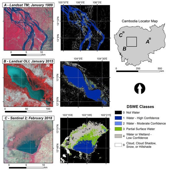
| Dataset Name | Class | Class Description |
|---|---|---|
| DSWE | 0 | Not water |
| 1 | Water—high confidence | |
| 2 | Water—moderate confidence | |
| 3 | Partial surface water pixel | |
| 4 | Water or wetland—low confidence | |
| 9 | Cloud, cloud shadow, or snow | |
| JRC | 0 | No data |
| 1 | Not water | |
| 2 | Water |
| 1989 Confusion Matrix | 1989 Landsat-Interpreted Reference | |||
| Low/No Water (0 and 4) | Moderate Water (2 and 3) | High Water (1) | ||
| DSWE Classes | Low/No Water (0 and 4) | 226 | 28 | 7 |
| Moderate Water (2 and 3) | 3 | 2 | 0 | |
| High Water (1) | 2 | 0 | 29 | |
| 2015 Confusion Matrix | 2015 Landsat-Interpreted Reference | |||
| Low/No Water (0 and 4) | Moderate Water (2 and 3) | High Water (1) | ||
| DSWE Classes | Low/No Water (0 and 4) | 211 | 34 | 6 |
| Moderate Water (2 and 3) | 0 | 3 | 3 | |
| High Water (1) | 0 | 1 | 35 | |
| 2018 Confusion Matrix | 2018 Sentinel-2-Interpreted Reference | |||
| Low/No Water (0 and 4) | Moderate Water (2 and 3) | High Water (1) | ||
| DSWE Classes | Low/No Water (0 and 4) | 184 | 24 | 2 |
| Moderate Water (2 and 3) | 0 | 2 | 1 | |
| High Water (1) | 0 | 2 | 33 | |
© 2020 by the authors. Licensee MDPI, Basel, Switzerland. This article is an open access article distributed under the terms and conditions of the Creative Commons Attribution (CC BY) license (http://creativecommons.org/licenses/by/4.0/).
Share and Cite
Soulard, C.E.; Walker, J.J.; Petrakis, R.E. Implementation of a Surface Water Extent Model in Cambodia using Cloud-Based Remote Sensing. Remote Sens. 2020, 12, 984. https://doi.org/10.3390/rs12060984
Soulard CE, Walker JJ, Petrakis RE. Implementation of a Surface Water Extent Model in Cambodia using Cloud-Based Remote Sensing. Remote Sensing. 2020; 12(6):984. https://doi.org/10.3390/rs12060984
Chicago/Turabian StyleSoulard, Christopher E., Jessica J. Walker, and Roy E. Petrakis. 2020. "Implementation of a Surface Water Extent Model in Cambodia using Cloud-Based Remote Sensing" Remote Sensing 12, no. 6: 984. https://doi.org/10.3390/rs12060984
APA StyleSoulard, C. E., Walker, J. J., & Petrakis, R. E. (2020). Implementation of a Surface Water Extent Model in Cambodia using Cloud-Based Remote Sensing. Remote Sensing, 12(6), 984. https://doi.org/10.3390/rs12060984