Article

Mapping Evapotranspiration, Vegetation and Precipitation Trends in the Catchment of the Shrinking Lake Poopó

by
Juan Torres-Batlló
1,
Belén Martí-Cardona
1,* and
Ramiro Pillco-Zolá
2
1
Department of Civil and Environmental Engineering, University of Surrey, Guildford GU2 7XH, UK
2
Instituto de Hidráulica e Hidrología, Universidad Mayor de San Andrés, La Paz, Bolivia
*
Author to whom correspondence should be addressed.
Remote Sens. 2020, 12(1), 73; https://doi.org/10.3390/rs12010073
Submission received: 30 October 2019 / Revised: 20 December 2019 / Accepted: 21 December 2019 / Published: 24 December 2019

Abstract

:
Lake Poopó is located in the Andean Mountain Range Plateau or Altiplano. A general decline in the lake water level has been observed in the last two decades, coinciding roughly with an intensification of agriculture exploitation, such as quinoa crops. Several factors have been linked with the shrinkage of the lake, including climate change, increased irrigation, mining extraction and population growth. Being an endorheic catchment, evapotranspiration (ET) losses are expected to be the main water output mechanism and previous studies demonstrated ET increases using Earth observation (EO) data. In this study, we seek to build upon these earlier findings by analyzing an ET time series dataset of higher spatial and temporal resolution, in conjunction with land cover and precipitation data. More specifically, we performed a spatio-temporal analysis, focusing on wet and dry periods, that showed that ET changes occur primarily in the wet period, while the dry period is approximately stationary. An analysis of vegetation trends performed using 500 MODIS vegetation index products (NDVI) also showed an overall increasing trend during the wet period. Analysis of NDVI and ET across land cover types showed that only croplands had experienced an increase in NDVI and ET losses, while natural covers showed either constant or decreasing NDVI trends together with increases in ET. The larger increase in vegetation and ET losses over agricultural regions, strongly suggests that cropping practices exacerbated water losses in these areas. This quantification provides essential information for the sustainable planning of water resources and land uses in the catchment. Finally, we examined the spatio-temporal trends of the precipitation using the newly available Climate Hazards Group Infrared Precipitation with Stations (CHIRPS-v2) product, which we validated with onsite rainfall measurements. When integrated over the entire catchment, precipitation and ET showed an average increasing trend of 5.2 mm yr−1 and 4.3 mm yr−1, respectively. This result suggests that, despite the increased ET losses, the catchment-wide water storage should have been offset by the higher precipitation. However, this result is only applicable to the catchment-wide water balance, and the location of water may have been altered (e.g., by river abstractions or by the creation of impoundments) to the detriment of the Lake Poopó downstream.

Graphical Abstract

1. Introduction

Endorheic or terminal catchments, i.e., those with no surface drainage to rivers or oceans constitute 25% of the world’s continental area (excluding Greenland and Antarctica) and are mostly located in semi-arid and arid climates [1]. Given the lack of outlet drainage, the surface water storage in endorheic catchments depends critically on the equilibrium among precipitation, evapotranspiration (ET) and groundwater exchange [2,3,4]. This equilibrium is affected, for example, by increases in agricultural land and irrigation, which intensifies ET water losses. ET and evaporation from open water surfaces may also be exacerbated by warming temperatures. Climate change combined with human activity has caused severe perturbances in the water balance of several endorheic basins around the world, leading to the shrinkage of their terminal lakes [4,5], such as Lake Urmia in Iran [6,7], the Aral Sea in Kazahkstan and Uzbekistan [8,9], Lake Chad in Central Africa [10] and the Great Salt Lake in the USA [5].
The Altiplano, in the Andean Mountain Range, is an endorheic, semi-arid catchment and the second largest mountain plateau in the world. Several studies have highlighted the vulnerability of the Altiplano’s water resources to climate change. For example, López-Moreno et al. [11] and Hunziker et al. [12] documented temperature increases in the Altiplano in the order of 0.20 °C decade−1 for the periods 1965–2012 and 1981–2010, respectively. Hoffmann and Requena [13] estimated the impact of long-term temperature increments on water resources in the northern part of the Altiplano and concluded that it would lead to a dramatic reduction of water in lakes, rivers, glaciers and wetlands, especially during the dry season. Other studies [14], using time-series of satellite images, revealed a 43% reduction of the total glacial cover in the Bolivian Andean Mountains in the period 1986–2014, which has given rise to new and potentially dangerous proglacial lakes. Vuille et al. [15] projected a decrease in water availability due to the retreat of Tropical Andean glaciers and the consequent decrease of their reservoir effect. Using global and regional climate models [16,17,18], some studies predicted changes in precipitation patterns that would lead to the intensification of floods and droughts in the area. In addition to climate change, anthropogenic activities have increased the pressure on the Altiplano’s water resources and are likely to exacerbate it further in the future. For example, annual quinoa yield, for which the Altiplano is a major producer, escalated from 28,500 to 75,500 tonnes in Bolivia between 2008 and 2014 [19]. Satgé et al. [20] showed increasing ET rates over cropland in the Altiplano between 2000 and 2014, suggesting its connection to the agriculture intensification. According to Buytaert and De Bièvre [21] the projected population growth in the tropical Andes will increase water demand by up to 50% in 2050. Based on population projections and glacio-hydrological simulations, several scenarios of increase in water demand in Bolivia from 2011 to 2039 of magnitudes ranging from 15% to 53% have been observed [22]. Mining, which is one of the main economic activities in the area, has increased significantly during the last decade leading to the release of heavy metals and other pollutants into the water bodies, thus impairing soil productivity, local fauna and human water use [23,24].
Lake Poopó, at the South East of the Andean Altiplano, is a shallow saline lake which supports livestock and fishing activities of local communities [20,25,26]. More than half of Lake Poopó’s annual input comes from the Desaguadero River, which originates from Lake Titicaca’s overflow. Apart from rare overspills towards the Laca Jahuira River, on the southwest of the lake [26,27], the major water loss mechanism of Lake Poopó is evaporation. The Desaguadero River and Poopó’s catchments undergo pronounced wet and dry seasons, causing a rapid recharge of Lake Poopó during the wet season, and a slower decline of water levels as the evaporation exceeds the inflows in the dry season [25]. The annual maximum and minimum lake extents strongly depends on the annual precipitation, as shown by Satgé et al. [20]. As a result of this dependency, Lake Poopó dried completely on several occasions in the past after severe dry episodes, e.g., in the early 1940’s, 1970’s, mid–1990’s and late 2015 [25].
Apart from the above mentioned specific extreme dry periods, some authors have claimed a declining trend in Lake Poopó water storage in the last two decades [20,28]. Satgé et al. [20] highlighted the clear decoupling of the lake extent from the annual precipitation in 2013 and 2014. Several studies have related the lake’s decline to the abovementioned pressures over the Altiplano water resources: rapid expansion of arable land in the catchment and an associated increase of ET losses [20]; the decreasing flow discharge in the Desaguadero River, presumably linked to irrigation uses [25,29,30], and the increased evaporation due to climate warming [11,29].
The lack of substantial ground-based hydro-meteorological observations and the large extent of the study area lead to the use of remote sensing data techniques to map and monitor the Altiplano water resources trends. Earth observation satellites have imaged the Earth periodically since the 1970s. These images can be processed to derive a wide range of spatial information of paramount relevance for water resource monitoring, such as the extent of water bodies [31,32,33,34,35], the spatial distribution of rainfall [36,37,38], inland water surface temperature [39,40,41,42], vegetation indexes [43,44,45,46,47,48] and ET dynamics [49,50,51,52,53], among others.
Satgé et al. [20] used monthly satellite products to assess ET losses over the Altiplano for the period 2000–2014 and pointed at the ET increase from cropland as a potential driver of Lake Poopó’s decline. The highest increases in ET were located in the northern part of the Desaguadero-Poopó (DP) system, despite the maximum cropland expansion being reported at the south and southwest of Lake Poopó by Jacobsen et al. [54] and Ayaviri and Vallejos [55]. So far, there is no integrated assessment of ET and vegetation tendencies for the study area. A better understanding of the interconnection among those factors is critical to tackle jointly land use and water resources planning.
The study presented here builds on the critical findings on ET trends by Satgé et al. [20] and extends those by using improved and more frequent ET products. Furthermore, we undertook, for the first time, an integrated assessment of vegetation, ET losses and precipitation spatio-temporal trends over the DP system. The study exploits the improved ET product from the National Aeronautics and Space Administration (NASA) obtained by the Moderate Resolution Imaging Spectroradiometer (MODIS, MOD16A2.006 Global Terrestrial Evapotranspiration 8–Day Global 500 m; [53]) together with MODIS Terra and Aqua vegetation index product (MOD13Q1.006 and MYD13Q1.006 16–Day Global 250 m; [56,57]) and Climate Hazards Group InfraRed Precipitation with Station Data (CHIRPS [58]) precipitation product. The processing was conducted using the new cloud-based Google Earth Engine, which enabled the integration of the complete time series of daily and 8-day products for the period of analysis, involving over 5000 raster datasets.
Temporal trends of vegetation, ET and precipitation were mapped for the entire study period, which encompassed the sharp increase in quinoa yield. The trends for the wet and dry seasons were also analysed independently for the first time. An additional novelty of this study is the characterization of ET and vegetation trends and absolute values for the broad land uses and geographical areas in the Altiplano. Although absolute values must be taken with caution due to their limited validation over the study area, their temporal trends are robust, and they represent the relative water consumption among different land covers. This information is of paramount relevance for the sustainable land use planning and management of water resources in the Altiplano. It is worth noting that, although final figures of precipitation inputs and ET outputs are provided for the entire system, a water balance was not attempted and the main conclusions are drawn from the comparison of the reliable temporal trends of those parameters.

2. Materials and Methods

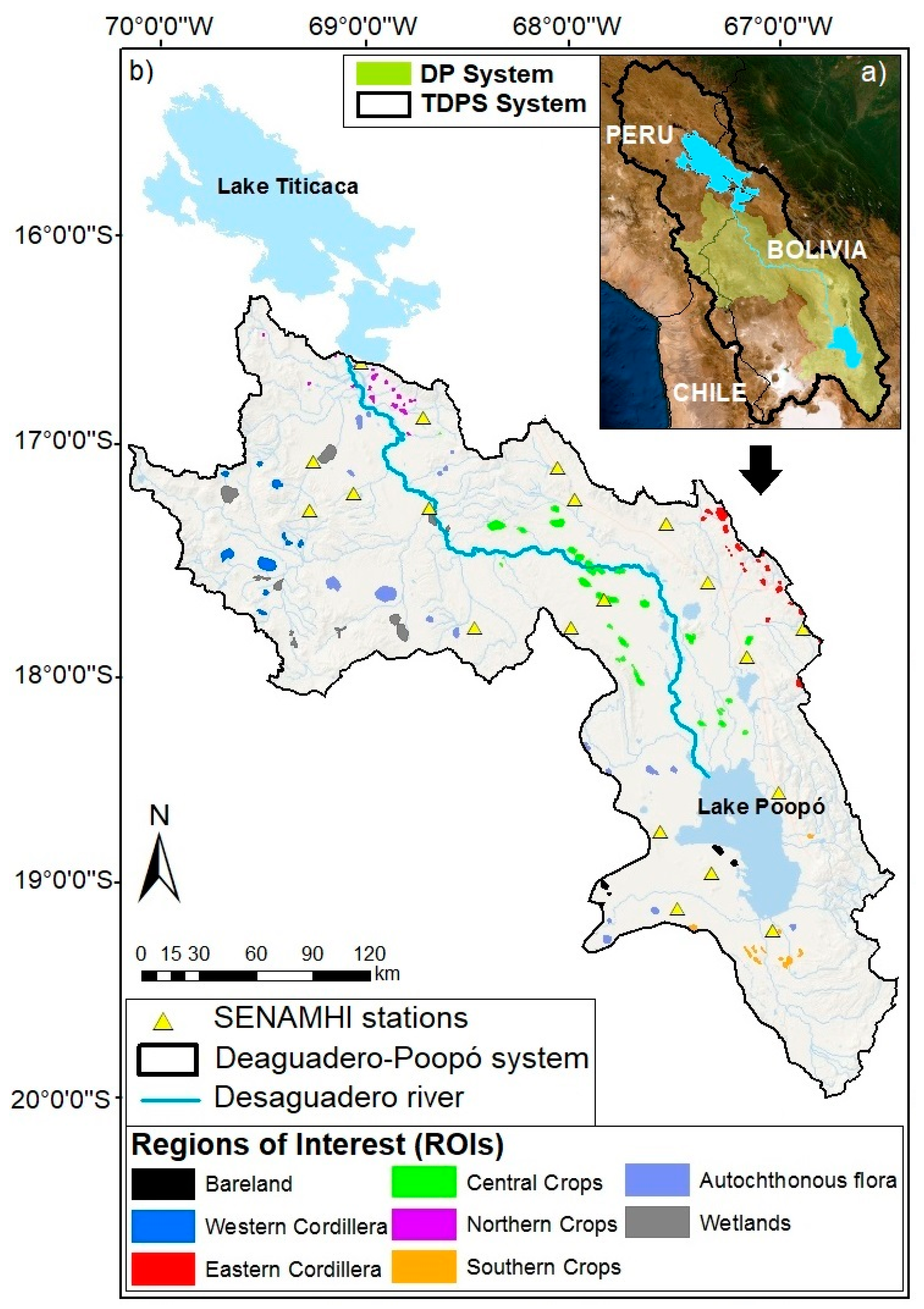
2.1. Study Area and Period

The Andean Altiplano is the second largest mountain plateau on the Earth after the Tibetan Plateau. It has an approximate area of 192,000 km2 at an average elevation of 4000 m, distributed over the countries as follows: Chile (4%), Peru (26%) and Bolivia (70%). The highest point is Mount Sajama (6542 m) and the lowest is at the bottom of Lake Titicaca (3533 m) [59]. It is one of the poorest regions in South America with a total population of 2.2 million [59].
Two large lakes lay on the Altiplano: Titicaca and Poopó (Figure 1). Lake Titicaca feeds the Desaguadero River which ends at Lake Poopó, contributing approximately 65% of its water volume [25]. This research will focus on the DP system which is the surface catchment contributing runoff to Lake Poopó. The DP has an area of approximately 58,000 km2 at a mean terrain elevation of 3810 m, limited by Lake Titicaca to the north, Cordillera Occidental to the south west and Cordillera Real to the north east (separates the DP from the Amazon basin). The DP is virtually an endorheic system with rare overspill discharge events towards Salar de Uyuni [26,27].
Annual precipitation varies with the latitude, ranging from about 750 mm yr−1 in the north to 160 mm yr−1 in the arid south. Rainfall is very unevenly distributed over the year, with 95% of the annual precipitation falling between October and March, while July and August are the driest months. The average annual temperatures are around 10 °C, achieving their minimum during the months of June and July and their peaks in the months of December and January. According to Pillco-Zolá et al. [60], the monthly average relative humidity varies between 52% and 68%. In terms of vegetation, 65% of the total vegetation area is covered by grassland followed by alpine vegetation (12%), crops (11%), bareland (9%) and wetland (3%). The most common crops in the Altiplano are potatoes and quinoa [54,61] being the area of largest quinoa production in the world.
This study analysed the vegetation, ET and precipitation spatio-temporal trends in the DP system for the period 2002–2014. The years 2015 and 2016 were excluded from the analysis due to the occurrence of an extreme El Niño phenomenon, which significantly altered the hydrological trends. The analysis was carried out encompassing the entire period from 2002 to 2014, and also focusing on the wettest months, January and February, and the driest ones, July and August. The overall and seasonal trends were mapped over the entire DP system, and also examined independently for the main land cover types.

2.2. Experimental Data

The remote sensing products and on-site records used in this study are listed in Table 1. Most of the analyses were carried out using the Google Earth Engine (GEE) platform [62], which enabled the effective access and processing of large spatio-temporal datasets.

2.2.1. Satellite Data

Two identical MODIS instruments are installed on board the Terra and Aqua satellites of the NASA, each imaging the entire Earth twice daily. Optimal quality pixels (i.e., with no sub-pixel cloud, low aerosol nor sensor view angle <30 degrees) from consecutive MODIS images are selected and used to produce vegetation index maps at 8-day intervals, made available as products MOD13Q1 and MYD13Q1 [56,57]. For the analysis of vegetation trends in the DP system, this study used the normalized difference vegetation index [63]. The accuracy of the MOD13Q1 and MYD13Q1 NDVI values for clear pixels is reported as ±0.025 [64].
Global actual and potential ET (ET, ETp) estimates are also derived from MODIS images combined with ancillary datasets and made available at 8-day intervals as product MOD16A2 [53,65]. ET estimates account for the actual (as opposed to potential) evaporation from canopy and soil, and for the real transpiration through plant´s stomata, and are provided in mm day−1. This study used ET and ETp product MOD16A2 version 6, which improves the previous version 5 in spatial resolution, from 1000 m to 500 m, and in the accuracy of near real-time surface weather data. It has been validated for 232 watersheds and 46 eddy flux towers [53], and its accuracy has been assessed with an average mean absolute error of about 24%, within the 10%–30% range of accuracy of ground ET observations [53,66,67].
MODIS surface reflectance [68] data was acquired for 16 May 2012, at the end of the wettest season in the study period, to generate a water mask. Table 1 summarizes the satellite data used in this study.

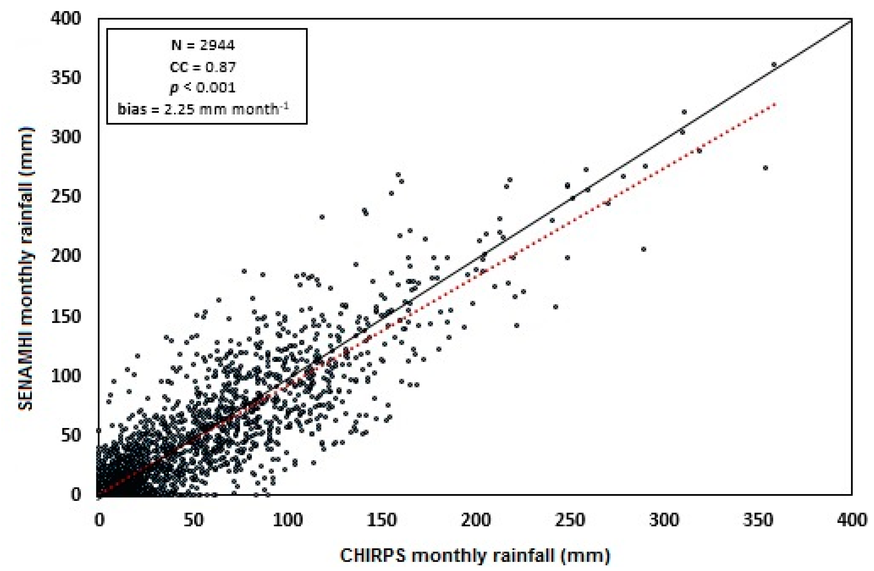
2.2.2. Precipitation Data

Precipitation data were collected from on-site meteorological stations and from satellite rainfall estimation products. Monthly precipitation data were obtained from twenty-one meteorological stations of the Servicio Nacional de Meteorología e Hidrología de Bolivia (SENAMHI). Figure 1 shows the location of these stations, which is sparse and not representative of high-elevation areas. In order to retrieve measurements from areas poorly gauged by meteorological stations, satellite precipitation estimations from CHIRPS were used. CHIRPS is a global rainfall dataset at 0.05 arc degree resolution, derived from satellite and in-situ precipitation measurements, developed by the U.S. Geological Survey (USGS) and the Climate Hazards Group [58]. CHIRPS precipitation data were successfully validated in areas adjacent to the DP system [69,70]. Here, monthly accumulated precipitation from each on-site meteorological station was compared to the one provided by its corresponding CHIRPS pixel. Figure 2 depicts the scatter plot for the two datasets, with a Spearman’s correlation coefficient (CC) of 0.87 with significant results and bias of 2.25 mm month−1 (Figure 2). Given the agreement between the two datasets, the regional analysis of precipitation was carried out using CHIRPS data, which provides full coverage of the DP system. A bias correction was not applied since only the precipitation temporal trends, and not their absolute values, were needed for the purpose of this study. The lack of precipitation ground data for the validation of the CHIRPS product over the highest parts of the DP system is acknowledged as a source of uncertainty, and current efforts are in place to improve their gauging.

2.2.3. Topography Model and Land Cover Map

Topographic data for the DP system was obtained from the Shuttle Radar Topography Mission (SRTM) terrain elevation model [71]. The terrain topography was used to delineate the DP watershed boundaries, to inform the delineation of control regions and to interpret the study results. The study used the version 3.0 with 30-m of spatial resolution and an absolute vertical accuracy of ~9 m (90% confidence) or better [72].
The land cover map Mapa de Cobertura y Uso Actual de la Tierra en Bolivia, COBUSO-2010 [73], was used to inform the delineation of the control regions as explained in Section 2.3. Commissioned by the Bolivian Government, COBUSO-2010 is a country-wide, 30-m spatial resolution land cover map derived from 60 Landsat 5 scenes acquired between 2006 and 2010. This map contains 21 different land cover types within the DP system.

2.3. Definition of Control Areas for the Main Land Cover Types

In order to associate the mean ET and NDVI magnitudes and trends to the main land cover types in the DP system and to explore their relative trends, eight broad land cover categories were defined based on the COBUSO-2010 classes. These categories and the COBUSO-2010 classes that they correspond to are briefly described below.
  • Northern Crops corresponds to cropland areas located in the northern part of the system, which were under exploitation long before 2002, the beginning of the study period. Northern Crops comprises Multiple Crops extracted from COBUSO-2010.
  • Central Crops represents agricultural areas located in the central valley of the DP system on alluvial soils and rather flat topography following the course of the Desaguadero River, grouping Multiple Crops from COBUSO-2010. Besides Multiple Crops, some residual pixels belonging to Central Crops are classified as Semi-arid Grassland and Wetland in COBUSO-2010.
  • Southern Crops are located south of Lake Poopó and encompass the COBUSO-2010 land cover of Multiple Crops.
  • Cordillera Real groups Multiple Crops, Sub-humid Andean Forest, Scattered Vivacious High-Andean Vegetation and Semi-arid Grassland located above 4200 m. All the covers are included in the same category, since their mixture occurs at a scale difficult to separate at the ET product resolution. An abundance of irrigation systems has been reported in this area by Canedo et al. [61] together with an expansion of the mining activity [23].
  • Cordillera Occidental includes Scattered Vivacious High-Andean Vegetation and Scattered Puna in Sand areas in the North West mountain range.
  • Autochthonous Flora encompasses Semi-arid Grassland, Scattered Puna in Sand areas, Scattered Vivacious High-Andean Vegetation and Sand Deposits in rare occurrences.
  • Wetland areas are located in the northern and northwestern part of the system due to the high availability of water. These areas represent flood zones with unique ecosystems and encompasses Wet Grasslands.
  • Bareland groups Sand, Sault and Lacustrine deposits with almost no vegetation. The highest extent of bareland is found in the arid south and southwest of the DP system.
Regions of interest (ROIs) were delineated for each of these categories (Figure 1) and validated by site visits and by visual inspection of multi-temporal, high-resolution Google Earth images. Google Earth Engine Timelapse [62], was used to ensure that the ROI’s land cover types had not changed during the study period. The ROIs were used to extract per-class NDVI and ET annual values and trends as explained in Section 3.3.

2.4. Masking Water Pixels

A MODIS surface reflectance image from 16 May 2012 was used to calculate the modified normalized difference water index (MNDWI) [74] over the entire DP system. A safe threshold of –0.3 was applied in order to identify likely waterlogged pixels and produce the MNDWI water mask. This mask was applied to the MODIS NDVI products prior to any analysis. It was not applied to the ET products since a water mask is already incorporated in their derivation. The May 2012 image was selected for the derivation of a water mask because it was acquired at the end of an extremely wet season, so it is expected to capture water bodies and prone-to-flood areas at a close-to-peak water extent condition. A constant water mask, as opposed to a time-varying one, was used for simplicity, although it may miss few, sporadic water-logged pixels.

2.5. Retrieval and Mapping of Vegetation, ET and Precipitation Trends

Per pixel annual averages of NDVI, ET losses and precipitation were calculated for the study period, using the entire dataset of the corresponding MODIS products. Per pixel ET, NDVI and precipitation temporal trends and their significance were assessed by calculating the Sen’s slope estimator [75] and Mann-Kendall (MK) test [76,77] as explained in the Section 2.5.1. Both, trend slope and MK test were applied to per-pixel data using the entire study period, and also considering the wet and dry seasons independently. The approach of the study is based on how physical processes change over time. This is the reason why the trend analysis was carried out under the assumption that the datasets follow a long-term persistence viewpoint.
NDVI, ET and precipitation average values and trends were mapped over the entire DP system and analysed together with the digital elevation model to identify physiographical regions exhibiting different temporal patterns. Average values and trends of NDVI, ET and precipitation were averaged within the ROIs representative of the main land cover types, to identify differential behaviours among them.

2.5.1. Calculation of Trends and Their Significance

Tests for the detection of trends in time series can be classified as parametric and non-parametric methods. Non-parametric tests do not presume the data distribution, only require them to be statistically independent [78]. Ordinary least squares (OLS) has been widely used to estimate linear trends. However, this method assumes normality in the dataset distribution. A common alternative to the simple linear regression method, for spatio-temporal vegetation and hydro-climatological analysis, has been the Sen’s slope estimator [78,79,80,81,82,83]. Sen’s slope is a non-parametric method which has been defined as a powerful tool, alternative to OLS, presenting more robustness to the outliers than the simple linear regression. The Sen’s slope is defined as the median of all possible slopes between pairs of two-dimensional sample points and it is calculated as follows:
Q = M e d i a n { x j x i j i } ,   for   i = 1 ,   ,   N ,
where Q is the slope, xj and xi are the values at time j and i (j > i), respectively, and N is the number of time periods representing the totality of the observations per pixel. Each point is compared with all the next data points and the median of the slopes is used to characterize the trend. Positive values indicate increasing trends while negative values indicate decreasing trends. The significance of the time series trends was evaluated by the non-parametric MK test [77,78]. The MK is one of the widely used non-parametric test to detect monotonic trends of hydro-meteorological data series [84,85,86,87,88]. Due to the study analyses hydrological data which is not normally distributed, non-parametric methods are well suited for the detection of monotonic trends. The following equations show how to calculate the test statistic S and the test statistic Z from the MK test:
S =   i = 1 n 1 j = i + 1 n s g n ( x j x i ) ,
s g n   ( x j x i ) = { 1 , i f x j x i < 0   0 , i f x x i = 0 + 1 , i f x x i > 0 ,
where n is the length of the dataset, xj and xi represent data points in time series j and i, respectively (j > i). The difference of the magnitude from each pair of values is compared (xj − xi) when (j > i) following Equation (3). Sgn (xj − xi) is the function sign whose value can be −1, 0 or 1. A positive S value means that the trend is increasing while a negative S value means that the trend is decreasing. The variance of S is estimated by the following equation:
V a r   ( S ) =   [ n ( n 1 ) ( 2 n + 5 ) j 1 g t j ( t j 1 ) ( 2 t j + 5 ) ] 18 ,
where g is the number of the tied groups in the data and tj is the number of data points in each tied group. The significance of the trend can be found calculating Z value, which is acquired as follows:
Z = { S 1 V a r ( S ) , S > 0           0 ,       S = 0 S + 1 V a r ( S ) ,   S < 0 .
In the present study, the significant level of Z was assessed at 99%, 95% and 90% intervals of confidence for |Z| values higher than 2.58, 1.96 and 1.64, respectively. Goodman [89] shows in Table 1 “Bayesian Interpretation of P–values” the correspondence between Z–score and the p-value. The MK test was assessed in all the NDVI, ET and precipitation spatio-temporal trend analysis.

3. Results

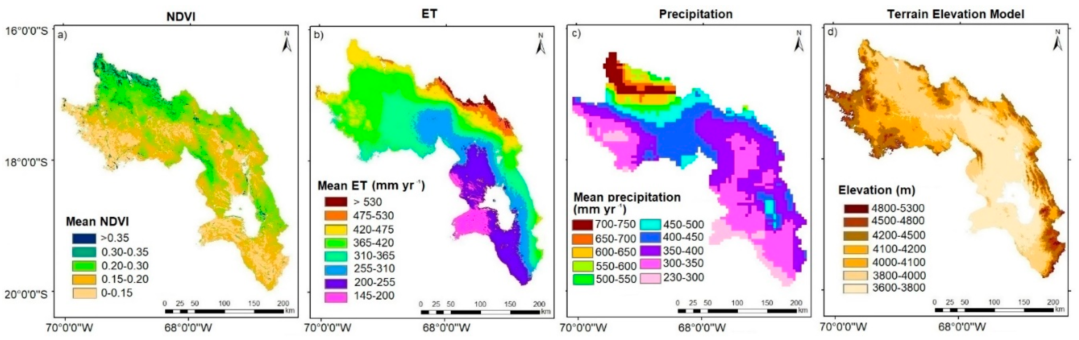
3.1. Average NDVI, ET and Precipitation Maps

NDVI values averaged for the study period (Figure 3a) range between 0.10 and 0.35 for virtually the entire DP system. The greenest area, with mean NDVI values from 0.25 to 0.35, is located at the north end of the catchment and encompasses dense agricultural developments and areas prone to flooding. The lowest vegetation index values are mainly concentrated at the south of Lake Poopó and in the mountainous north-west, coinciding roughly with the areas of lowest precipitation. The average ET losses range from 145 to 550 mm yr−1 (Figure 3b). They appear to be closely related to the terrain elevation (Figure 3d), increasing more rapidly with elevation over the Cordillera Real. The maximum ET values are observed in high elevation areas of the Cordillera Real, followed by the northernmost part, where NDVI values are the highest. The lowest ET losses occur in the drier south part, with average annual values under 250 mm yr−1. An acute north-south gradient is observed in the spatial distribution of precipitation, with annual values ranging from 750 mm yr−1 in the north to 230 mm yr−1 in the south (Figure 3c). A detailed analysis of precipitation patterns in the DP system can be found in Garreaud, et al. [90] and Pillco et al. [91].

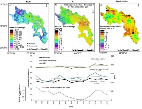
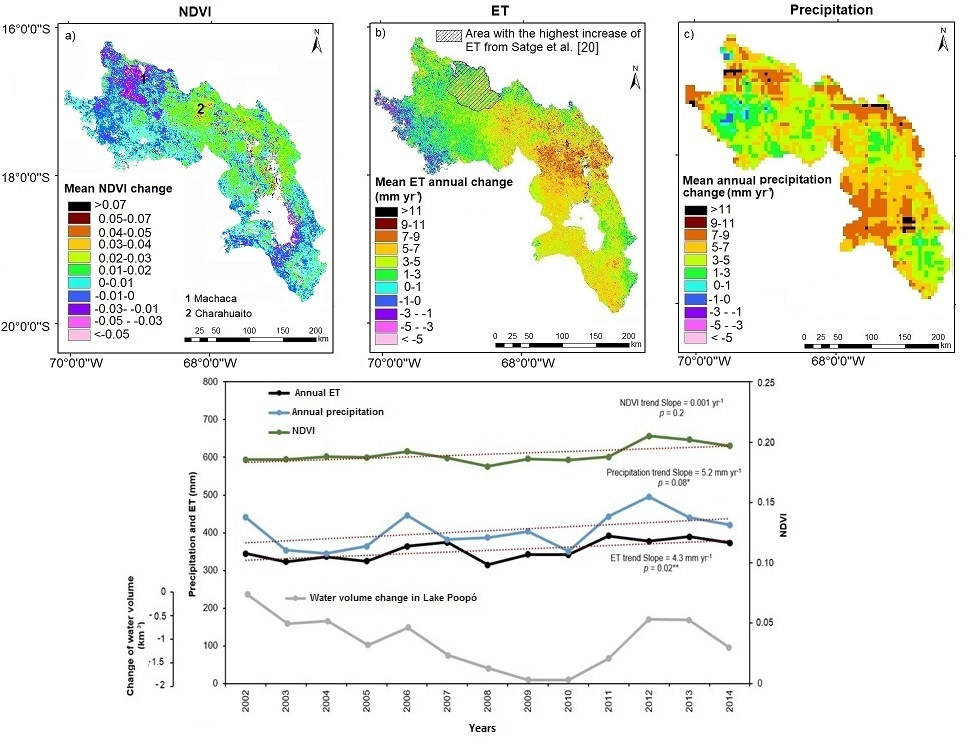
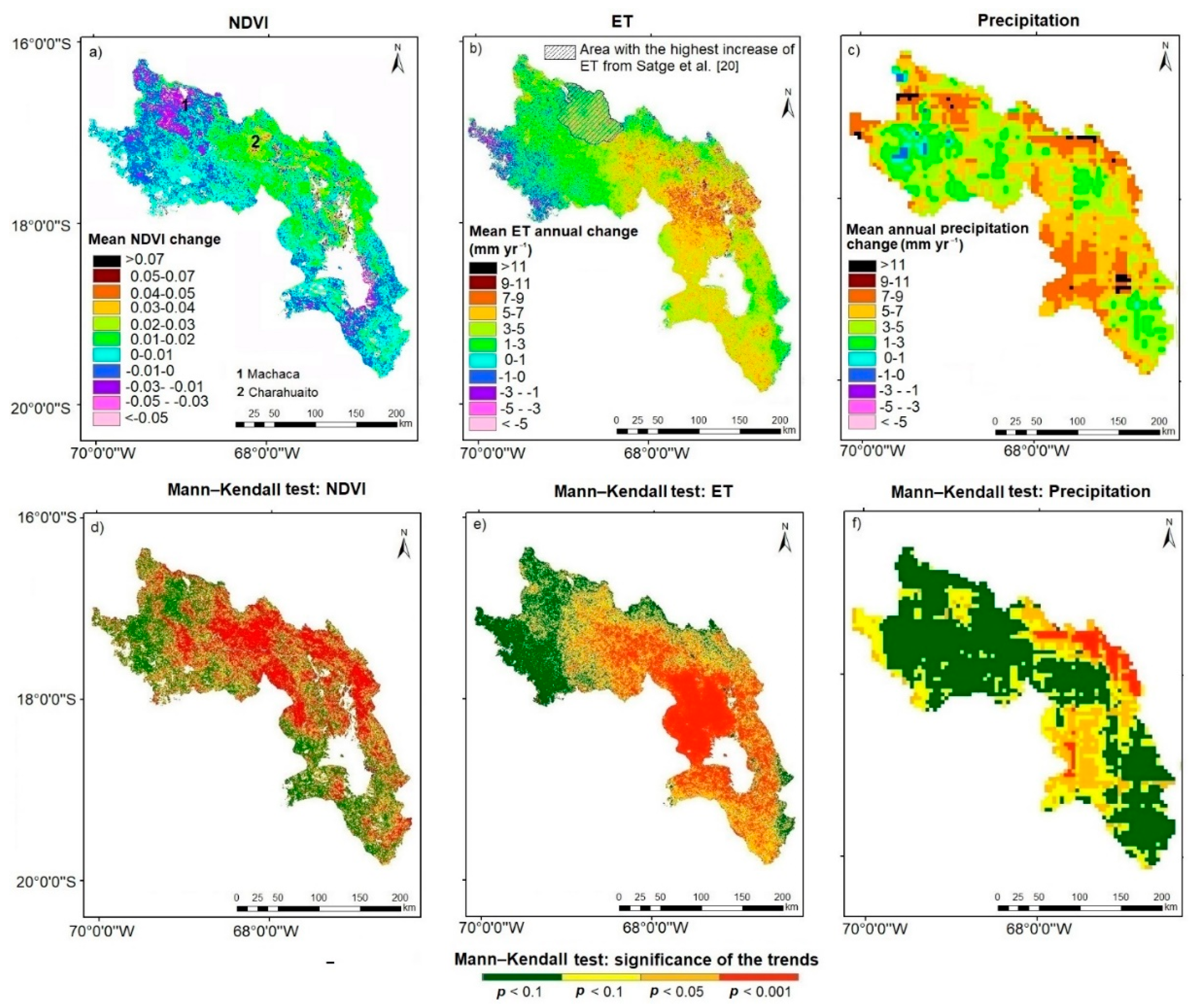
3.2. Spatio-Temporal Trends in NDVI, ET and Precipitation

Figure 4 depicts the mean annual NDVI, the annual accumulated ET and ETp and annual precipitation integrated over the entire DP system for every year in the study period together, with the change of water volume in Lake Poopó. The ET and precipitation time series show a mean increasing trend of 4.3 mm yr−1 and 5.2 mm yr−1 at significance confidence levels of 90% and 95%, respectively. The catchment-wide NDVI exhibits a slower and not-significant increasing trend, mimicking to some degree the rainfall temporal pattern. ETp shows an increasing trend of 1.59 mm yr−1 without significance levels.
Figure 5 illustrates the spatial distribution of the analysed temporal changes and their per-pixel significance. Figure 5a shows that per-pixel vegetation changes across the entire period were small over most of the catchment. Two clusters of NDVI trends can be identified: one corresponds to the areas around Charahuaito (see Figure 5a) in the southwest part of Aroma province, exhibiting the largest positive NDVI change rate; the second cluster is located at the north end of the system, close to Machaca, and exhibits a negative trend. Both clusters correspond to the areas with the highest mean NDVI (Figure 3).
The spatial distribution of ET temporal trends reveals highly significant increments over a large central part of the system (Figure 5b), while the clearer negative trends are concentrated on the mountainous north-west area. Higher increasing trends were observed in precipitation than in ET over the DP system, especially in the eastern and central parts of the system. No clear spatial correlations between the NDVI and ET trends have been identified.
Some differences were observed in the spatial distribution of increasing ET trends when compared with those reported by Satgé et al. [20]. The authors observed statistically significant ET increases in the north of the catchment (see hatched area in Figure 5b). In our research, the highest increases were observed over a larger, central part of the system. Significant increases were also observed in the south, where the expansion of quinoa crops was reported [51].
When considering seasonal temporal trends, the wet season presents statistically significant increases in NDVI, ET and precipitation, whereas the dry season shows no changes or slight decreases (Table 2, Figure 6). In the wet season, NDVI increments occur largely over areas of high mean NDVI. The greatest precipitation increases were observed in mountainous areas over the wet season.

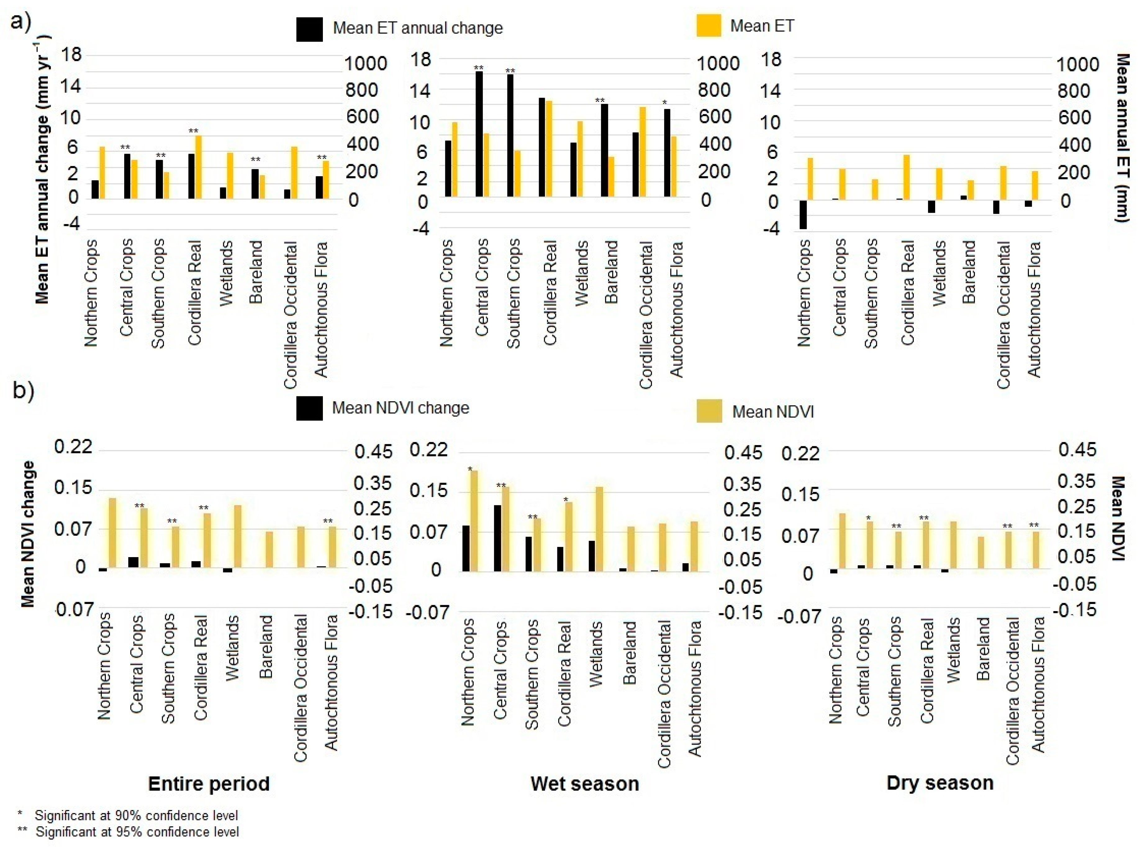
3.3. Analysis of ET and NDVI Trends Per Land Cover Type

Figure 7 depicts the ET and NDVI mean values and mean change rate for the analysed land cover types. The results reveal that change trends were positive in virtually all cases except for the dry season and that the largest increases occurred in the wet season for all cover types. Table 3 shows the significance confidence level of the land cover trends.
The results of the vegetation land cover analysis revealed interesting and comparable patterns of seasonal vegetation trends. Over the period 2002–2014, land cover NDVI trends were generally positive across the DP system (see Figure 7b), especially during the wet season. As in the ET analysis, the land cover presenting the highest increases was Central Crops. Greater increases for Northern Crops and Southern Crops than for Cordillera Real were noticed during the wet season. Wetland was the land cover without human activity that presented higher increases during the wet season, followed by Autochthonous flora. Cordillera Occidental and Bareland did not present significant changes in their dynamics for the entire period. No remarkable changes were noticed during the dry season in all the land covers. Wetland and Northern Crops were the only land covers showing negative trends during the entire period.

4. Discussion

Recent years have shown a decreasing trend in the water levels of Lake Poopó coinciding with an intensification of agriculture practices [19,20,54], mining activity [23,24], urban growth [21] and a regional increase in the temperatures [11,12]. The study presented here focused on the detailed temporal analysis of the spatially distributed parameters: ET, precipitation and vegetation. Due to the complexity of the system, we did not attempt to explain all issues affecting Lake Poopó, but to exploit state-of-the-art spatio-temporal data to improve our quantitative knowledge of one of the factors that has been highlighted by recent literature as a possible driver of the lake’s decline: the increased ET losses.

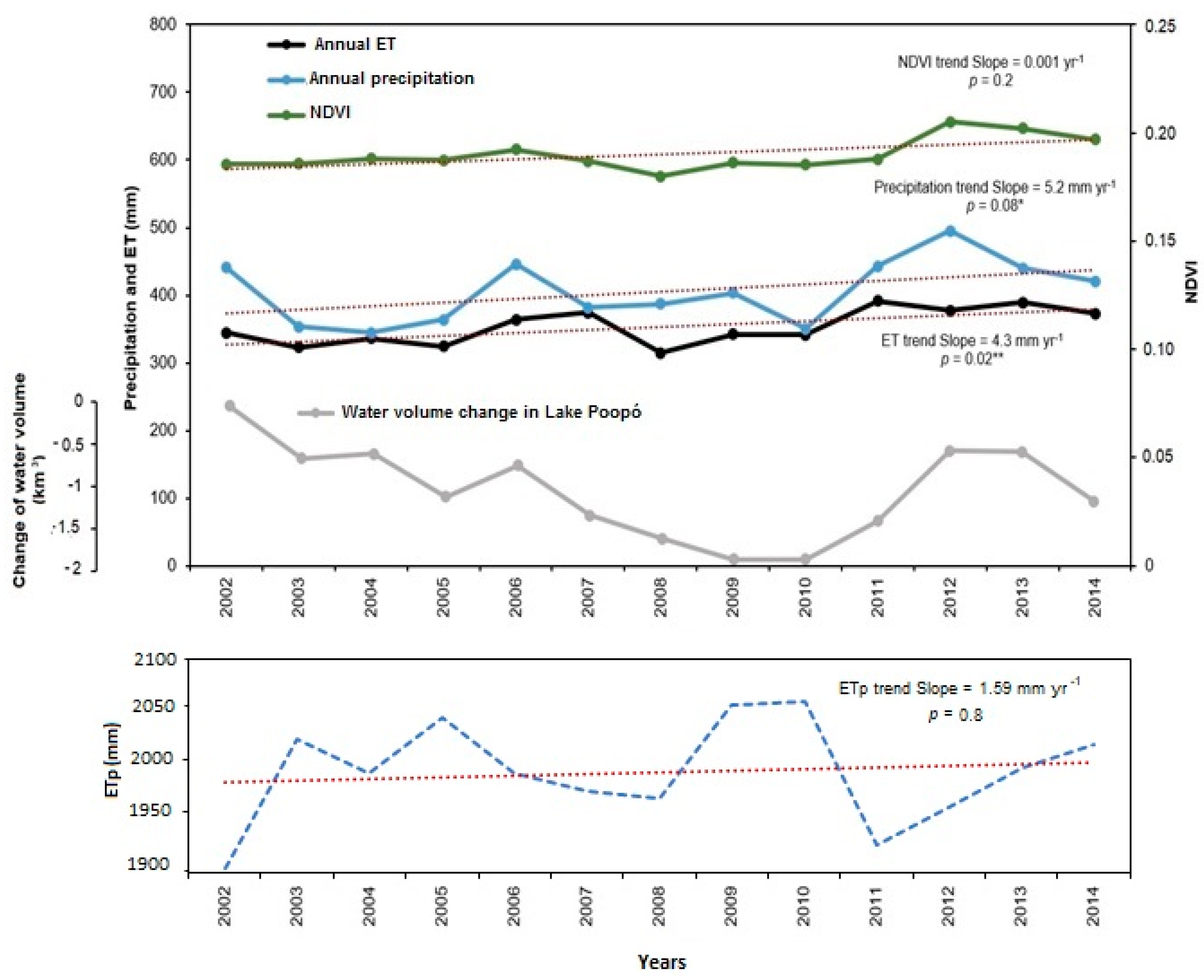
4.1. Temporal Assessment of ET, Precipitation and NDVI at the Catchment Scale

From a catchment water balance point of view, our results indicate that the overall increase in actual ET (average rate of 4.3 mm yr−1) was compensated by the overall increase in precipitation (average rate of 5.2 mm yr−1) during the analysed period, both trends being statistically significant. This suggests that the ET is not to blame for depleting the DP system of water. It is likely though, that the water paths and water storage location have been altered (e.g., due to river abstractions for irrigation [30] and by impounding upstream tributaries of the lake [93]) in detriment of the downstream recipient, which is Lake Poopó.
The catchment aggregated ETp losses showed an increasing trend (average rate of 1.6 mm yr−1) clearly lower than the ET trend. This result strongly suggests that the ET increases are not only driven by climatic changes, as already pointed out by Satgé et al. [20]. However, the ETp trends should be interpreted with caution since both, Satgé et al.’s and ours, showed very low significance values.
The analysis regarding the temporal trend of the NDVI indicated an increase of 0.013 for the entire period which may be influenced by the intensification in agriculture and irrigation practices [54] and also by the effect of increased precipitation over natural vegetation.

4.2. Spatial Distribution of ET, Precipitation and NDVI Trends

Given previous literature linking the increased ET losses in the DP system to farming and irrigation and the fact that irrigated crops in arid regions normally show higher vegetation indices than the surrounding landscape, it was initially expected to find a spatial consistency between ET and NDVI increases. However, such relationship was not clear. For instance, in the northern part of the system, around Machaca (see Figure 5b), an NDVI decrease coincides with an ET increase, while both ET and NDVI increased comparably around Charahuaito. The analysis of ETp located the largest increases in the north of the DP system, including the area around Machaca. This observation seems consistent with Seiler et al. [94] results, who indicated that the highest temperature increments in Bolivia for the period 1965–2004 had occurred in the north of the DP system. This observation suggests that climate trends have played a significant role in exacerbating the water losses in that specific area.
Some differences regarding the spatial distribution of ET trends between the study by Satgé et al. [20] and the one presented here were observed and illustrated in Figure 5b. This discrepancy is due to the different MODIS ET product used. While Satgé et al. [20] used approximately 180 ET products at monthly intervals for the period 2000–2014, this study used a total of 598 ET products at eight-day intervals, from 2002 to 2014. Furthermore, Satgé et al. [20] analysis used the MODIS ET product version 5, at a spatial resolution of 1000 m, whereas this research benefitted from the latest version 6, which is an upgrade of the same product, at a spatial resolution of 500 m. Despite the mentioned discrepancy in the location of the highest ET increases, both studies report similar magnitudes of the ET trends. They also agree in the location of the main ET decreases in the north-west mountains of the DP system. However, unlike [20], our results indicate that the largest ET increases occurred in the central and southern part of the DP system, reaching average rates of 7 to 13 mm yr−1. The identified areas include new agriculture exploitations, such as Quinoa crops south of Lake Poopó, new irrigation systems in the Cordillera Real [61], and also includes the vicinities of the city of Oruro, which has experienced considerable growth in the last decade, including new roads which may alter the natural runoff pathways, as revealed by satellite imagery. These areas are also where the largest increment of actual ET versus ETp was found. More spatially focused studies would be needed to investigate the specific causes behind the observed increases in order to take the appropriate actions.
The seasonal analysis of ET, NDVI and precipitation spatial trends consistently indicated that the dry periods were mainly stationary, while the largest and most significant changes occurred during the wet seasons.

4.3. ET and NDVI Trends Per Land Cover Type

The results revealed that among the analysed land cover classes only those including crops, i.e., Central Crops, Southern Crops and Cordillera Real, experienced an increase in both, NDVI and ET losses, with the only exception of Northern Crops. Additionally, they were the cover types with the highest increases in ET. This results strongly suggest that cropping practices, such as reported irrigation in the central part of the system and Cordillera Real [61], or the expansion of quinoa crops at the south of Lake Poopó [54], exacerbated water losses on these regions. Natural covers showed either constant or decreasing NDVI trends together with increases in ET. This is most likely caused by the observed increase in temperatures due to climate change [11,12] and in precipitation.
The land cover analysis quantified the relative water consumption among the selected broad cover types. This quantification provides essential information for the sustainable planning of land use and water resources in the DP system, since it informs of the expected increments in water consumption associated to planned land use transformations, such as crop expansions (e.g., the Bolivian National Development Plan proposes 1.5 million hectares of new irrigated cropland for 2030) or reforestation [93]. For example, according to our results, the conversion from autochthonous flora to cropland areas would increase the annual water consumption by 7% when located in the central part of the system, and by 41% when located within the Cordillera Real. Thus, the ET figures obtained in this research help estimate the impact of land use transformations in the DP system on the Lake Poopó’s water balance. It has to be noticed, however, that the land covers defined here were rather broad, and that future research can further refine the obtained ET figures for more specific cover types and locations within the DP system.

5. Conclusions

With the aim of exploring catchment changes that may have impacted the Lake Poopó water balance, this study has undertaken a comprehensive spatio-temporal analysis of changes in vegetation, ET losses and precipitation over the DP system for the period 2002–2014, using more than 5000 satellite products. Temporal trends of these parameters have also been quantified for the main land cover classes in the area. The main conclusions stemming from this study are as follows:
  • The spatio-temporal analysis confirmed an increase of ET losses between 2002 and 2014 within the DP system, although our study showed the maximum increases of ET losses over the central area of the catchment, differing from previous studies.
  • The NDVI and ET values averaged annually over the DP system increased at a mean rate of 0.001 yr−1 and 4.3 mm yr−1, which yields mean NDVI and annual ET increments of 0.013 and 56 mm for the 13-year study period. Water inputs into the system due to precipitation increased at a mean rate of 5.2 mm yr−1, exceeding the ET rise rate.
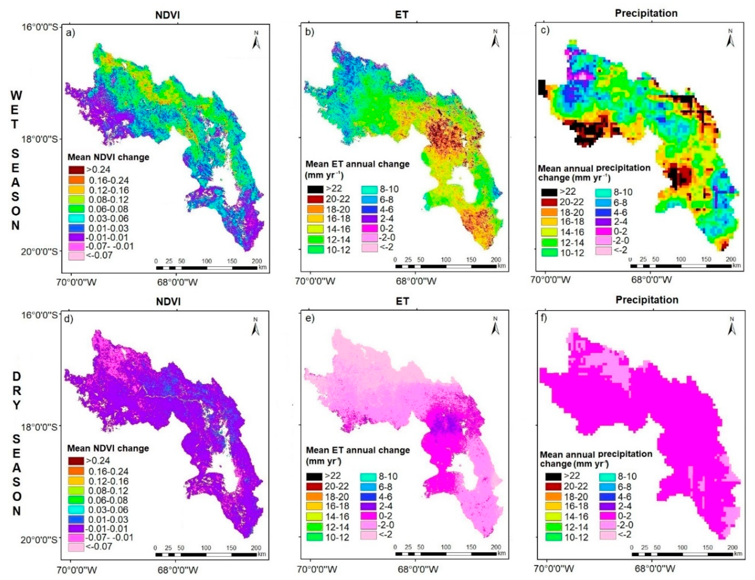
  • The seasonal analysis revealed that the highest ET and NDVI changes occur during the wet period contrasting with the stationarity of the dry period.
  • ET losses and their trends have been estimated for the main land covers in the DP catchment. Their values indicate that the land covers with higher water consumption are: Cordillera Real, Cordillera Occidental, Northern Crops, Wetlands and Central Crops with average values of 500, 410, 410, 370 and 310 mm yr−1, respectively. This quantification of water consumption per cover type provides crucial information for the sustainable planning of agriculture exploitation and water resources use in the DP system.
  • Among the analysed land cover classes, only those including crops, such as Central and Southern Crops and Cordillera Real, have experienced an increase in NDVI and ET losses, while natural covers showed either constant or decreasing NDVI trends together with increases in ET. The larger increase in NDVI and ET losses over agricultural regions, strongly suggests that cropping practices exacerbated water losses in these areas.
These results indicate that overall water availability has not decreased at the catchment scale and urge the investigation of trends in other lake water balance terms, such as the flow discharge in the Desaguadero River other tributaries, the evaporation losses and the water exchange between the lake and the aquifer.

Author Contributions

Data curation, J.T.-B. and B.M.-C.; Formal analysis, J.T.-B. and B.M.-C.; Investigation J.T.-B. and B.M.-C.; Methodology, J.T.-B.; Project administration, B.M.-C.; Resources, R.P.-Z., B.M.-C. and J.T.-B.; Software, J.T.-B.; Supervision, B.M.-C.; Writing—original draft J.T.-B.; Writing—review & editing, B.M.-C. All authors have read and agreed to the published version of the manuscript.

Funding

This research received no external funding.

Acknowledgments

The authors express their gratitude to USGS, Climate Hazard Group, and Google Earth Engine for the availability of the MODIS and CHIRPS datasets, and to SENAMHI (Bolivia) for the in situ precipitation data.

Conflicts of Interest

The authors declare no conflicts of interest.

References

  1. Hostetler, S.W. Hydrological and Thermal Response of Lakes to Climate: Description and Modeling; Springer: Berlin/Heidelberg, Germany, 1995; Volume 60, ISBN 3-540-57891-9. [Google Scholar]
  2. Hammer, U.T. Saline Lake Ecosystems of the World; Springer Science and Business Media: Amsterdam, The Netherlands, 1986; Volume 59, ISBN 978-90-6193-535-3. [Google Scholar]
  3. McCarthy, J.J.; Canziani, O.F.; Leary, N.A.; Dokken, D.J.; White, K.S. (Eds.) Climate Change 2001: Impacts, Adaptation, and Vulnerability; Contribution of Working Group II to the Third Assessment Report of the Intergovernmental Panel on Climate Change; Cambridge University Press: Cambridge, UK, 2001; Volume 2, ISBN 0-521-80768-9. [Google Scholar]
  4. Wang, J.; Song, C.; Reager, J.T.; Yao, F.; Famiglietti, J.S.; Sheng, Y.; MacDonald, G.M.; Brun, F.; Schmied, H.M.; Marston, R.A.; et al. Recent global decline in endorheic basin water storages. Nat. Geosci. 2018, 11, 926. [Google Scholar] [CrossRef] [PubMed] [Green Version]
  5. Wurtsbaugh, W.A.; Miller, C.; Null, S.E.; DeRose, R.J.; Wilcock, P.; Hahnenberger, M.; Moore, J. Decline of the world’s saline lakes. Nat. Geosci. 2017, 10, 816. [Google Scholar] [CrossRef]
  6. Eimanifar, A.; Mohebbi, F. Urmia Lake (northwest Iran): A brief review. Saline Syst. 2005, 3, 5. [Google Scholar] [CrossRef] [PubMed] [Green Version]
  7. AghaKouchak, A.; Norouzi, H.; Madani, K.; Mirchi, A.; Azarderakhsh, M.; Nazemi, A.; Nasrollahi, N.; Farahmand, A.; Mehran, A.; Hasanzadeh, E. Aral Sea syndrome desiccates Lake Urmia. call for action. J. Great Lakes Res. 2015, 41, 307–311. [Google Scholar] [CrossRef]
  8. Micklin, P. Desiccation of the Aral Sea. A Water Management Disaster in the Soviet Union. Science 1988, 241, 1170–1176. [Google Scholar] [CrossRef] [PubMed] [Green Version]
  9. Micklin, P. The Aral sea disaster. Annu. Rev. Earth Planet. Sci. 2007, 35, 47–72. [Google Scholar] [CrossRef] [Green Version]
  10. Gao, H.; Bohn, T.J.; Podest, E.; McDonald, K.C.; Lettenmaier, D.P. On the causes of the shrinking of Lake Chad. Environ. Res. Lett. 2011, 6, 034021. [Google Scholar] [CrossRef] [Green Version]
  11. López-Moreno, J.I.; Morán-Tejeda, E.; Vicente-Serrano, S.M.; Bazo, J.; Azorin-Molina, C.; Revuelto, J.; Sánchez-Lorenzo, A.; Navarro-Serrano, F.; Aguilar, E.; Chura, O. Recent temperature variability and change in the Altiplano of Bolivia and Peru. Int. J. Clim. 2015, 36, 1773–1796. [Google Scholar] [CrossRef] [Green Version]
  12. Hunziker, S.; Brönnimann, S.; Calle, J.; Moreno, I.; Andrade, M.; Ticona, L.; Huerta, A.; Lavado-Casimiro, W. Effects of undetected data quality issues on climatological analyses. Clim. Past. 2018, 14, 1–20. [Google Scholar] [CrossRef] [Green Version]
  13. Hoffmann, D.; Requena, C. Bolivia en un Mundo 4 Grados más Caliente: Escenarios Sociopolíticos Ante el Cambio Climático Para los Años 2030 y 2060 en el Altiplano Norte; Fundación PIEB, Programa de Investigación Estratégica en Bolivia: La Paz, Bolivia, 2012. [Google Scholar]
  14. Cook, S.J.; Kougkoulos, I.; Edwards, L.A.; Dortch, J.; Hoffmann, D. Glacier change and glacial lake outburst flood risk in the Bolivian Andes. Cryosphere 2016, 10, 2399–2413. [Google Scholar] [CrossRef] [Green Version]
  15. Vuille, M.; Francou, B.; Wagnon, P.; Juen, I.; Kaser, G.; Mark, B.G.; Bradley, R.S. Climate change and tropical Andean glaciers. Past, present and future. Earth Sci. Rev. 2008, 89, 79–96. [Google Scholar] [CrossRef] [Green Version]
  16. Thibeault, J.M.; Seth, A.; García, M. Changing climate in the Bolivian Altiplano. CMIP3 projections for temperature and precipitation extremes. J. Geophys. Res. Atmos. 2010, 115. [Google Scholar] [CrossRef]
  17. Seth, A.; Thibeault, J.; Garcia, M.; Valdivia, C. Making sense of twenty-first-century climate change in the Altiplano. Observed trends and CMIP3 projections. Ann. Assoc. Am. Geogr. 2010, 100, 835–847. [Google Scholar] [CrossRef]
  18. Urrutia, R.; Vuille, M. Climate change projections for the tropical Andes using a regional climate model. Temperature and precipitation simulations for the end of the 21st century. J. Geophys. Res. Atmos. 2009, 114. [Google Scholar] [CrossRef]
  19. Instituto Nacional de Estadística. Estadísticas Económicas; Instituto Nacional de Estadística, Ed.; The Bolivian National Institute of Statistics: La Paz, Bolivia, 2015. (In Spanish) [Google Scholar]
  20. Satgé, F.; Espinoza, R.; Zolá, R.P.; Roig, H.; Timouk, F.; Molina, J.; Garnier, J.; Calmant, F.; Seyler, F.; Bonnet, M.P. Role of climate variability and human activity on Poopó Lake droughts between 1990 and 2015 assessed using remote sensing data. Remote Sens. 2017, 9, 218. [Google Scholar] [CrossRef] [Green Version]
  21. Buytaert, W.; De Bièvre, B. Water for cities. The impact of climate change and demographic growth in the tropical Andes. Water Resour. Res. 2012, 48. [Google Scholar] [CrossRef] [Green Version]
  22. Kinouchi, T.; Nakajima, T.; Mendoza, J.; Fuchs, P.; Asaoka, Y. Water security in high mountain cities of the Andes under a growing population and climate change. A case study of La Paz and El Alto, Bolivia. Water Secur. 2019, 6, 100025. [Google Scholar] [CrossRef]
  23. Perreault, T. Dispossession by accumulation? Mining, water and the nature of enclosure on the Bolivian Altiplano. Antipode 2013, 45, 1050–1069. [Google Scholar] [CrossRef]
  24. Andreucci, D.; Radhuber, I. Limits to “counter-neoliberal” reform. Mining expansion and the marginalisation of post-extractivist forces in Evo Morales’s Bolivia. Geoforum 2017, 84, 280–291. [Google Scholar] [CrossRef]
  25. Zola, R.P.; Bengtsson, L. Long-term and extreme water level variations of the shallow Lake Poopó, Bolivia. Hydrol. Sci. J. 2006, 51, 98–114. [Google Scholar] [CrossRef] [Green Version]
  26. Zolá, R.P.; Bengtsson, L. Three methods for determining the area-depth relationship of Lake Poopó, a large shallow lake in Bolivia. Lakes and Reservoirs. Res. Manag. 2007, 12, 275–284. [Google Scholar] [CrossRef]
  27. Revollo, M.M. Management issues in the Lake Titicaca and Lake Poopo system. importance of developing a water budget. Lakes and Reservoirs. Res. Manag. 2001, 6, 225–229. [Google Scholar] [CrossRef]
  28. Arsen, A.; Crétaux, J.F.; Berge-Nguyen, M.; del Rio, R.A. Remote sensing-derived bathymetry of Lake Poopó. Remote Sens. 2014, 6, 407–420. [Google Scholar] [CrossRef] [Green Version]
  29. Abarca-Del-Rio, R.; Crétaux, J.F.; Berge-Nguyen, M.; Maisongrande, P. Does Lake Titicaca still control the Lake Poopó system water levels? An investigation using satellite altimetry and MODIS data (2000–2009). Remote Sens. Lett. 2012, 3, 707–714. [Google Scholar] [CrossRef]
  30. Molina Carpio, J.; Satgé, F.; Pillco Zola, R. Los Recursos Hídricos Del Sistema TDPS. Available online: http.//horizon.documentation.ird.fr/exl-doc/pleins_textes/divers14-09/010062840.pdf (accessed on 10 July 2017).
  31. Campbell, J.B.; Wynne, R.H. Introduction to Remote Sensing; Guilford Press: New York, NY, USA, 2011. [Google Scholar]
  32. Alsdorf, D.E.; Rodríguez, E.; Lettenmaier, D.P. Measuring surface water from space. Rev. Geophys. 2007, 45. [Google Scholar] [CrossRef]
  33. Marti-Cardona, B.; Lopez-Martinez, C.; Dolz-Ripolles, J.; Bladè-Castellet, E. ASAR polarimetric, multi-incidence angle and multitemporal characterization of Doñana wetlands for flood extent monitoring. Remote Sens. Environ. 2010, 114, 2802–2815. [Google Scholar] [CrossRef]
  34. Martí-Cardona, B.; Dolz-Ripollés, J.; López-Martínez, C. Wetland inundation monitoring by the synergistic use of ENVISAT/ASAR imagery and ancillary spatial data. Remote Sens. Environ. 2013, 139, 171–184. [Google Scholar] [CrossRef]
  35. Huang, C.; Chen, Y.; Zhang, S.; Wu, J. Detecting, extracting, and monitoring surface water from space using optical sensors. A review. Rev. Geophys. 2018, 56, 333–360. [Google Scholar] [CrossRef]
  36. Kidd, C. Satellite rainfall climatology. A review. Int. J. Clim. 2001, 21, 1041–1066. [Google Scholar] [CrossRef]
  37. Espinoza Villar, J.C.; Ronchail, J.; Guyot, J.L.; Cochonneau, G.; Naziano, F.; Lavado, W.; De Oliveira, E.; Pombosa, R.; Vauchel, P. Spatio-temporal rainfall variability in the Amazon basin countries (Brazil, Peru, Bolivia, Colombia, and Ecuador). International Journal of Climatology. Int. J. Clim. 2009, 29, 1574–1594. [Google Scholar] [CrossRef] [Green Version]
  38. Bookhagen, B.; Burbank, D.W. Toward a complete Himalayan hydrological budget. Spatiotemporal distribution of snowmelt and rainfall and their impact on river discharge. J. Geophys. Res. 2010, 115. [Google Scholar] [CrossRef] [Green Version]
  39. Schneider, P.; Hook, S.J. Space observations of inland water bodies show rapid surface warming since 1985. Geophys. Res. Lett. 2010, 37. [Google Scholar] [CrossRef] [Green Version]
  40. Crosman, E.T.; Horel, J.D. MODIS–derived surface temperature of the Great Salt Lake. Remote Sens. Environ. 2009, 113, 73–81. [Google Scholar] [CrossRef]
  41. Liu, G.; Ou, W.; Zhang, Y.; Wu, T.; Zhu, G.; Shi, K.; Qin, B. Validating and mapping surface water temperatures in Lake Taihu. Results from MODIS land surface temperature products. IEEE J. Sel. Top. Appl. 2015, 8, 1230–1244. [Google Scholar] [CrossRef]
  42. Martí-Cardona, B.; Prats, J.; Niclòs, R. Enhancing the retrieval of stream surface temperature from Landsat data. Remote Sens. Environ. 2019, 224, 182–191. [Google Scholar] [CrossRef] [Green Version]
  43. Chen, X.L.; Zhao, H.M.; Li, P.X.; Yin, Z.Y. Remote sensing image-based analysis of the relationship between urban heat island and land use/cover changes. Remote Sens. Environ. 2006, 104, 133–146. [Google Scholar] [CrossRef]
  44. Xie, Y.; Sha, Z.; Yu, M. Remote sensing imagery in vegetation mapping: A review. J. Plant Ecol. 2008, 1, 9–23. [Google Scholar] [CrossRef]
  45. Herrmann, S.M.; Anyamba, A.; Tucker, C.J. Recent trends in vegetation dynamics in the African Sahel and their relationship to climate. Glob. Environ. Chang. 2005, 15, 394–404. [Google Scholar] [CrossRef]
  46. de Jong, R.; de Bruin, S.; de Wit, A.; Schaepman, M.E.; Dent, D.L. Analysis of monotonic greening and browning trends from global NDVI time-series. Remote Sens. Environ. 2011, 115, 692–702. [Google Scholar] [CrossRef] [Green Version]
  47. Eckert, S.; Hüsler, F.; Liniger, H.; Hodel, E. Trend analysis of MODIS NDVI time series for detecting land degradation and regeneration in Mongolia. J. Arid. Environ. 2015, 113, 16–28. [Google Scholar] [CrossRef]
  48. Duethmann, D.; Blöschl, G. Why has catchment evaporation increased in the past 40 years? A data-based study in Austria. Hydrol. Earth Syst. Sci. 2018, 22, 5143–5158. [Google Scholar] [CrossRef] [Green Version]
  49. Courault, D.; Seguin, B.; Olioso, A. Review on estimation of evapotranspiration from remote sensing data. From empirical to numerical modeling approaches. Irrig. Drain 2005, 19, 223–249. [Google Scholar] [CrossRef]
  50. Karimi, P.; Bastiaanssen, W.G.M. Spatial evapotranspiration, rainfall and land use data in water accounting—Part 1. Review of the accuracy of the remote sensing data. Hydrol. Earth Syst. Sci. 2015, 19, 507–532. [Google Scholar] [CrossRef] [Green Version]
  51. Martí-Cardona, B.; Pipia, L.; Rodríguez Máñez, E.; Hans Sánchez, T. Teledetección de la Evapotranspiración y Cambio de Cubiertas en la Cuenca del Río Locumba, Perú. In XXVII Congreso Latinoamericano de Hidráulica; IAHR: Lima, Peru, 2016. [Google Scholar]
  52. Mo, X.; Chen, X.; Hu, S.; Liu, S.; Xia, J. Attributing regional trends of evapotranspiration and gross primary productivity with remote sensing: A case study in the North China Plain. Hydrol. Earth Syst. Sci. 2017, 21, 295–310. [Google Scholar] [CrossRef] [Green Version]
  53. Running, S.; Mu, Q.; Zhao, M. MOD16A2 MODIS/Terra Net Evapotranspiration 8–Day L4 Global 500 m SIN Grid V006. Nasa Eosdis Land Process. Daac 2017. [Google Scholar] [CrossRef]
  54. Jacobsen, S. The Situation for Quinoa and Its Production in Southern Bolivia. From Economic Success to Environmental Disaster. J. Agron. Crop. Sci. 2011, 197, 390–399. [Google Scholar] [CrossRef]
  55. Nina, D.A.; Mamani, P.V. Cambio climático y seguridad alimentaria, un análisis en la producción agrícola. J. De Cienc. Y Tecnol. Agrar. 2014, 3, 59–70. [Google Scholar]
  56. Didan, K. MOD13Q1 MODIS/Terra Vegetation Indices 16-Day L3 Global 250m SIN Grid V006. NASA Eosdis Land Process. DAAC 2015. [Google Scholar] [CrossRef]
  57. Didan, K. MYD13Q1 MODIS/Aqua Vegetation Indices 16-Day L3 Global 250m SIN Grid V006. NASA Eosdis Land Process. DAAC 2015. [Google Scholar] [CrossRef]
  58. Funk, C.; Peterson, P.; Landsfeld, M.; Pedreros, D.; Verdin, J.; Shukla, S.; Husak, G.; Rowland, J.; Harrison, L.; Hoell, A.; et al. The climate hazards infrared precipitation with stations—A new environmental record for monitoring extremes. Sci. Data 2015, 2, 150066. [Google Scholar] [CrossRef] [Green Version]
  59. OEA (Organización de los Estados Americanos). Diagnóstico Ambiental del Sistema Titicaca-Desaguadero-Poopó-Salar de Coipasa (Sistema TDPS) Bolivia-Perú; Departamento Regional y Medio Ambiente, OEA: Washington, DC, USA, 1996. [Google Scholar]
  60. Pillco Zolá, R.; Bengtsson, L.; Berndtsson, R.; Martí-Cardona, B.; Satgé, F.; Timouk, F.; Bonnet, M.-P.; Mollericon, L.; Gamarra, C.; Pasapera, J. Modelling Lake Titicaca’s daily and monthly evaporation. Hydrol. Earth Syst. Sci 2019, 23, 657–668. [Google Scholar] [CrossRef] [Green Version]
  61. Canedo, C.; Pillco Zolá, R.; Berndtsson, R. Role of Hydrological Studies for the Development of the TDP System. Water Sui. 2016, 8, 144. [Google Scholar] [CrossRef] [Green Version]
  62. Gorelick, N.; Hancher, M.; Dixon, M.; Ilyushchenko, S.; Thau, D.; Moore, R. Google Earth Engine. Planetary-scale geospatial analysis for everyone. Remote Sens. Environ. 2017, 202, 18–27. [Google Scholar] [CrossRef]
  63. Rouse, J.W.; Haas, R.H.; Schell, J.A.; Deering, D.W. Monitoring Vegetation Systems in the Great Plains with ERTS (Earth Resources Technology Satellite). In Proceedings of the Third Earth Resources Technology Satellite Symposium, Greenbelt, ON, Canada, 10–14 December 1973; Volume 1, pp. 309–317. [Google Scholar]
  64. Gao, X.; Huete, A.R.; Didan, K. Multisensor comparisons and validation of MODIS vegetation indices at the semiarid Jornada experimental range. IEEE Trans. Geosci. Remote 2003, 41, 2368–2381. [Google Scholar] [CrossRef]
  65. Mu, Q.; Zhao, M.; Running, S.W. Improvements to a MODIS global terrestrial evapotranspiration algorithm. Remote Sens. Environ. 2011, 115, 1781–1800. [Google Scholar] [CrossRef]
  66. Jiang, L.; Islam, S.; Carlson, T.N. Uncertainties in latent heat flux measurement and estimation. implications for using a simplified approach with remote sensing data. Can. J. Remote Sens. 2004, 30, 769–787. [Google Scholar] [CrossRef]
  67. Kalma, J.D.; McVicar, T.R.; McCabe, M.F. Estimating land surface evaporation. A review of methods using remotely sensed surface temperature data. Surv. Geophys. 2008, 29, 421–469. [Google Scholar] [CrossRef]
  68. Vermote, E. MOD09A1 MODIS/Terra Surface Reflectance 8-Day L3 Global 500m SIN Grid V006. NASA Eosdis Land Process. DAAC 2015, 10. [Google Scholar] [CrossRef]
  69. Satgé, F.; Ruelland, D.; Bonnet, M.-P.; Molina, J.; Pillco, R. Consistency of satellite-based precipitation products in space and over time compared with gauge observations and snow-hydrological modelling in the Lake Titicaca region. Hydrol. Earth Syst. Sci. 2019, 23, 595–619. [Google Scholar] [CrossRef] [Green Version]
  70. Canedo Rosso, C.; Hochrainer-Stigler, S.; Pflug, G.; Condori, B.; Berndtsson, R. Early warning and drought risk assessment for the Bolivian Altiplano agriculture using high resolution satellite imagery data. Nat. Hazards Earth Syst. Sci. Discuss. 2018. [Google Scholar] [CrossRef] [Green Version]
  71. Farr, T.G.; Rosen, P.A.; Caro, E.; Crippen, R.; Duren, R.; Hensley, S.; Kobrick, M.; Paller, M.; Rodriguez, E.; Roth, L.; et al. The shuttle radar topography mission. Rev. Geophys. 2007, 45. [Google Scholar] [CrossRef] [Green Version]
  72. Rodriguez, E.; Morris, C.S.; Belz, J.E.; Chapin, E.C.; Martin, J.M.; Daffer, W.; Hensley, S. An Assessment of the SRTM Topographic Products; Technical Report JPL D-31639; Jet Propulsion Laboratory: Pasadena, CA, USA, 2005. [Google Scholar]
  73. UTNIT. Mapa de Cobertura y uso Actual de la Tierra, Bolivia. COBUSO-2010. Unidad Tecnica Nacional de Informacion de la Tierra. Available online: http.//cdrnbolivia.org/geografia-fisica-nacional.html (accessed on 2 March 2018).
  74. Xu, H. Modification of normalised difference water index (NDWI) to enhance open water features in remotely sensed imagery. Int. J. Remote Sens. 2006, 27, 3025–3033. [Google Scholar] [CrossRef]
  75. Sen, P.K. Estimates of the regression coefficient based on Kendall’s tau. J. Am. Stat. Assoc. 1968, 63, 1379–1389. [Google Scholar] [CrossRef]
  76. Mann, H. Nonparametric Tests Against Trend. Econometrica 1957, 13, 245. [Google Scholar] [CrossRef]
  77. Kendall, M.G. Rank Correlation Methods; Charles Griffin and Company Limited: London, UK, 1975. [Google Scholar]
  78. Gocic, M.; Trajkovic, S. Analysis of changes in meteorological variables using Mann-Kendall and Sen’s slope estimator statistical tests in Serbia. Glob. Planet. Chang. 2013, 100, 172–182. [Google Scholar] [CrossRef]
  79. Yue, S.; Pilon, P.; Cavadias, G. Power of the Mann-Kendall and Spearman’s rho tests for detecting monotonic trends in hydrological series. J. Hydrol. 2002, 259, 254–271. [Google Scholar] [CrossRef]
  80. Neeti, N.; Eastman, J.R. A contextual mann-kendall approach for the assessment of trend significance in image time series. Trans. GIS 2011, 15, 599–611. [Google Scholar] [CrossRef]
  81. Guay, K.C.; Beck, P.S.; Berner, L.T.; Goetz, S.J.; Baccini, A.; Buermann, W. Vegetation productivity patterns at high northern latitudes: A multi-sensor satellite data assessment. Glob. Chang. Biol. 2014, 20, 3147–3158. [Google Scholar] [CrossRef]
  82. Fernandes, R.; Leblanc, S.G. Parametric (modified least squares) and non-parametric (Theil-Sen) linear regressions for predicting biophysical parameters in the presence of measurement errors. Remote Sens. Environ. 2005, 95, 303–316. [Google Scholar] [CrossRef]
  83. Wu, Z.; Wu, J.; Liu, J.; He, B.; Lei, T.; Wang, Q. Increasing terrestrial vegetation activity of ecological restoration program in the Beijing-Tianjin Sand Source Region of China. Ecol. Eng. 2013, 52, 37–50. [Google Scholar] [CrossRef]
  84. Dinpashoh, Y.; Jhajharia, D.; Fakheri-Fard, A.; Singh, V.P.; Kahya, E. Trends in reference crop evapotranspiration over Iran. J. Hydrol. 2011, 399, 422–433. [Google Scholar] [CrossRef]
  85. Shadmani, M.; Marofi, S.; Roknian, M. Trend analysis in reference evapotranspiration using Mann-Kendall and Spearman’s Rho tests in arid regions of Iran. Water Resourc. Manag. 2012, 26, 211–224. [Google Scholar] [CrossRef] [Green Version]
  86. Fensholt, R.; Proud, S.R. Evaluation of earth observation based global long term vegetation trends—Comparing GIMMS and MODIS global NDVI time series. Remote Sens. Environ. 2012, 119, 131–147. [Google Scholar] [CrossRef]
  87. Fang, N.F.; Chen, F.X.; Zhang, H.Y.; Wang, Y.X.; Shi, Z.H. Effects of cultivation and reforestation on suspended sediment concentrations: A case study in a mountainous catchment in China. Hydrol. Earth Syst. Sci. 2016, 20, 13–25. [Google Scholar] [CrossRef] [Green Version]
  88. Fathian, F.; Dehghan, Z.; Bazrkar, M.H.; Eslamian, S. Trends in hydrological and climatic variables affected by four variations of the Mann-Kendall approach in Urmia Lake basin, Iran. Hydrol. Sci. J. 2016, 61, 892–904. [Google Scholar] [CrossRef] [Green Version]
  89. Goodman, S.N. Of P-values and Bayes: A modest proposal. Epidemiology 2001, 12, 295–297. [Google Scholar] [CrossRef]
  90. Garreaud, R.; Vuille, M.; Clement, A.C. The climate of the Altiplano: Observed current conditions and mechanisms of past changes. Palaegeogr. Palaeocl. 2003, 194, 5–22. [Google Scholar] [CrossRef] [Green Version]
  91. Pillco, R.; Uvo, C.B.; Bengtsson, L.; Villegas, R. Precipitation variability and regionalization over the Southern Altiplano, Bolivia. Int. J. Clim. 2007, 149–164. [Google Scholar]
  92. Cretaux, J.-F.; Jelinski, W.; Calmant, S.; Kouraev, A.V.; Vuglinski, V.V.; Bergé Nguyen, M.; Gennero, M.-C.; Nino, F.; Abarca-Del-Rio, R.; Cazenave, A.; et al. SOLS: A lake database to monitor in Near Real Time water level and storage variations from remote sensing data. J. Adv. Space Res. 2011, 47, 1497–1507. [Google Scholar] [CrossRef]
  93. Estado Plurinacional de Bolivia. El Plan de Desarrollo Económico y Social; Ministerio de Planificación de Desarrollo: La Paz, Bolivia, 2016. [Google Scholar]
  94. Seiler, C.; Hutjes, R.W.; Kabat, P. Climate variability and trends in Bolivia. J. Appl. Meteorol. 2013, 52, 130–146. [Google Scholar] [CrossRef] [Green Version]
Figure 1. Study area indicating: (a) the location of the Titicaca-Desaguadero-Poopó-Salares (TDPS) system within the South American continent; and the DP system within the TDPS; (b) the Desaguadero-Poopó (DP) system, the Regions of Interest (ROIs) representative of land cover types (see Section 2.3 for land-cover definitions) and the location of meteorological stations.
Remotesensing 12 00073 g001
Figure 2. Scatter plot of monthly rainfall estimates from Climate Hazards Group InfraRed Precipitation with Station Data (CHIRPS) versus in-situ measurements from Servicio Nacional de Meteorología e Hidrología (SENAMHI) stations.
Remotesensing 12 00073 g002
Figure 3. Spatial distribution of mean NDVI, ET and precipitation for the period 2002–2014 and terrain elevation of the DP system. (a) Mean NDVI; (b) Mean ET; (c) Mean annual precipitation; (d) Terrain elevation.
Remotesensing 12 00073 g003
Figure 4. Evolution and temporal trends of ET, Potential ET (ETp), precipitation and mean NDVI over the entire DP system, and volume change in Lake Poopó [92].
Remotesensing 12 00073 g004
Figure 5. Spatial distribution of NDVI, ET and precipitation trends during the study period: (a) Mean NDVI change (calculated as the mean trend multiplied by the duration of the study period); (b) Mean ET trend; (c) Mean precipitation trends. (df) show the spatial distribution of the significance level of the trends for the period 2002–2014 in the DP system. Red, orange and yellow colours indicate significant results.
Remotesensing 12 00073 g005
Figure 6. NDVI, ET and precipitation seasonal trends over the DP system for the period 2002–2014: Mean NDVI change (calculated as the mean trend multiplied by the duration of the study period) for (a) wet season and (d) dry season; ET mean annual change for (b) wet season and (e) dry season; and precipitation mean annual change for (c) wet season and (f) dry season.
Remotesensing 12 00073 g006
Figure 7. Mean trends and absolute values of ET and NDVI per land cover type and significance level of the trends: (a) Mean ET trend (mm yr−1) and mean annual ET (mm); (b) mean NDVI change (calculated as the mean trend multiplied by the duration of the study period) and mean NDVI.
Remotesensing 12 00073 g007
Table 1. Datasets used in this study.
PRODUCT NAMEMOD16A2MOD13Q1MYD13Q1MOD09A1SRTMCHIRPS
Physical magnitudeEvapotranspiration (ET)NDVINDVIReflectanceTerrain elevationPrecipitation
Spatial resolution500 m250 m250 m500 m30 m0.05 arc degrees
Temporal interval8 days16 days16 days8 daysN/ADaily
Number of products used 16 May 2012Mosaic of 10 granules
Entire study period598299288 4748
Wet season1055248 770
Dry season1045252 806
Table 2. Regional annual ET mean changes in the DP System from 2002 to 2014. NDVI mean change for the study period 2002–2014. Statistics obtained from the non-parametric Mann-Kendall test.
Wet PeriodDry Period
NDVIETPrecipitationNDVIETPrecipitation
Sen’s slope0.04910.7 mm yr−113.26 mm yr−10.002−0.7 mm yr−10.26 mm yr−1
p value 0.06 *0.03 **0.06 *0.02 **0.240.15
Significant pixels51%66%40%70%20%28%
* Significant at 90% confidence level. ** Significant at 95% confidence level.
Table 3. Result of the Mann-Kendall (MK) test for the land cover type trend analysis.
NDVIET
Land Cover TypesEntire PeriodWet PeriodDry PeriodEntire PeriodWet PeriodDry Period
Bareland0.420.340.360.01 **0.03 **0.38
Wetlands0.30.330.320.210.330.44
Cordillera Occ.0.240.280.01 **0.360.320.24
Cordillera Orient.0.03 **0.06 *0.00 **0.03 **0.260.36
Autochthonous Flora0.01 **0.160.03 **0.04 **0.09 *0.21
Northern Crops0.140.09 *0.220.110.180.34
Central Crops0.00 **0.00 **0.08 *0.00 **0.02 **0.48
Southern Crops0.00 **0.00 **0.00 **0.02 **0.02 **0.42
* Significant at 90% confidence level. ** Significant at 95% confidence level.

